Spectral Analysis of Stationary Signals Based on Two Simplified Arrangements of Chirp Transform Spectrometer

Abstract

The classical two-channel push-pull chirp transform spectrometer (CTS) has been widely applied in satellite-borne remote sensing systems for earth observation and deep space exploration. In this paper, we present two simplified structures with single M(l)-C(s) CTS arrangements for the spectral analysis of stationary signals. A simplified CTS system with a single M(l)-C(s) arrangement and a time delay line was firstly developed. Another simplified structure of CTS with a M(l)-C(s) arrangement and a frequency conversion channel was also developed for spectral analysis of stationary signals. Simulation and experiment results demonstrate that the two simplified arrangements can both realize spectrum measurement for the stationary signals and obtain the same frequency resolution, amplitude accuracy and system sensitivity as that of the classical two-channel push–pull CTS system. Compared to the classical CTS structure, the two simplified arrangements require fewer devices, save power consumption and have reduced mass. The matching problem between the two channels can be avoided in the two simplified arrangements. The simplified CTS arrangements may have potential application in the spectrum measurement of stationary signals in the field of aviation and spaceflight.

1. Introduction

Signal-processing techniques based on the chirp transform algorithm [1] have been developed and used for several decades [2,3]. With the development of the radar pulse compression technology and the high-performance surface acoustic wave (SAW) filter [4], chirp transform techniques have been widely used to perform real-time Fourier transform. Based on chirp transform techniques, the analog Fourier transform system is called the chirp transform spectrometer (CTS) [5,6,7].

The main feature of the CTS system is the analog SAW filter, which is used as the convolver for matched filtering. Initially designed for pulse compression in a radar system, the SAW filter was developed rapidly and is available commercially with up to 800 MHz bandwidth [8]. The large operational bandwidth of the SAW filter gives the CTS system large real-time processing bandwidth and high spectral resolution. Compared to the established fast-Fourier-transform (FFT) spectrometer [9], the CTS system with the analog SAW filter as the convolver offers high resolution, high stability, low power consumption, low mass and small size at the expense of limited accuracy and dynamic range [10]. Many significant breakthroughs in the design of the SAW filters with large time–bandwidth product as well as precise dispersive matching between the SAW devices have promoted the implementation of the CTS system [11]. The CTS system has been widely developed and applied in many fields, such as microwave remote sensing, meteorological sounding, astronomical observations as well as deep space exploration [12]. Early in the 1990s, the CTS backend was used for atmosphere sounding by P. Hartogh [13,14]. In the mid-1990s, the ground-based CTS system was used for the sub-millimeter observations of comets [15] and planets [16]. The CTS backend has also been used in the Microwave Spectrometer for the Rosetta Orbiter (MIRO), which launched in 2004 and has investigated the atmosphere of Comet Chyruymov Gerasimenko since 2014. Recently, the CTS backend has been applied in the high-resolution spectrometer of the German Receiver for Astronomy at Terahertz Frequency (GREAT) on board the Stratospheric Observatory For Infrared Astronomy (SOFIA) for the study of modern astrophysics.

In a CTS system, the main features of the chirp transform algorithm are the signal expansion and pulse compression. In [10], it is shown that the premultiplication of the measured signal with a chirp signal (signal expansion) followed by a convolution filter (signal compression) and then postmultiplication with another chirp signal yields the Fourier transform. The spectral distribution of the measured signal can be found though the time distribution of the output pulses. There are usually two similar arrangements in a CTS system. One is the M(S)-C(l)-M arrangement, in which the time duration of the premultiplication chirp signal is short compared to the impulse response of the convolution filter. Another is the M(l)-C(s)-M arrangement, in which the time duration of the premultiplication chirp signal is long. The used notation M denotes the multiplication, C denotes the convolution, l means long duration time and s means short duration time. If only considering the power spectrum of the stationary signal, the procedure of the postmultiplication with another chirp signal can be ignored, which means that only the M-C arrangement obtains the same results as the M-C-M arrangement. Taking the frequency resolution and the process of the SAW convolution filter into consideration, it is more advisable to use the M(l)-C(s) arrangement for Fourier transform processor design.

The M(l)-C(s) arrangement is also called the sliding transform and actually analyzes the spectrum of the input signal at different time segments, and thus it is only suitable for the measurement of the stationary signal. Meanwhile, the time segmentation measurement of the input signal can only observe part of the spectrum, influencing the system sensitivity. To improve the system sensitivity, a classical two-channel push-pull CTS structure with two M(l)-C(s) arrangements was developed [17]. This two-channel push-pull CST structure has two symmetrical M(l)-C(s) arrangements, which have a half-period time delay between each other. It can measure the stationary signal and obtain the maximum system sensitivity. The biggest challenge of the two-channel CTS structure is the matching problem between the two channels (especially the match between different SAW filters), which directly influences the accuracy of the power spectrum and the frequency resolution. In this research, we studied and developed two novel simplified structures with only one M(l)-C(s) arrangement for the measurement of the stationary signal. These two simplified structures have fewer devices and less weight and can avoid the matching problem without degrading the system’s performance.

The contents of this paper are organized as follows. In Section 2, we firstly give a brief introduction to the M(l)-C(s) arrangement and its operational principle, followed by some application limitations. Subsequently, the classical two-channel push-pull CTS system that based on two M(l)-C(s) arrangements is presented and discussed. In Section 3, two simplified CTS structures based on only one M(l)-C(s) arrangement for the measurement of stationary signals are presented and theoretically analyzed individually. The simulation and experimental verification of the two novel simplified structures are presented in Section 4 and Section 5. We also discuss the benefits and drawbacks of the two simplified structures compared to the classical two-channel structure from the system structure to the system performance, including the power spectrum and frequency resolution of the output pulses. A brief conclusion is drawn in the last section.

2. M-C Arrangement and the Classical Two-Channel CTS System

2.1. M(l)-C(s) Arrangement

Usually, a symmetrical structure (M-C-M or C-M-C arrangements) is required to perform a full Fourier transform. When only considering the power spectrum of the measured signal, the M(l)-C(s) arrangement can obtain the same result as the symmetrical structure. Figure 1 is the sketch of the M(l)-C(s) arrangement. The expander chirp signal $C_1\left(t\right)$ that used for the premultiplication is generated by an analog SAW filter or by direct digital synthesis (DDS) devices. The convolution filter (also called the matching filter) is an analog SAW filter, which has a dispersive characteristic opposite to that of the expander chirp signal. The expander chirp signal $C_1\left(t\right)$ and the impulse response of the convolution filter $H_0\left(t\right)$ are both of the form

$$C_1\left(t\right)={\displaystyle \prod \left\{\frac{t-t_1}{T_1}\right\}}{w}_1\left(t\right)\cdot \cos \left({\omega }_{1}t-\pi \mu t^2+{\varphi }_1\right)$$

(1)

Equation (1) describes a finite time and bandwidth-duration chirp signal, where ${\displaystyle \prod \left\{\frac{t-t_1}{T_1}\right\}}$ is a rectangular gating function with time duration $T_1$ centered on time $t=t_1$. Function $w_1\left(t\right)$ is an arbitrary weighting function, and it is set to be unity in the following derivation. ${\omega }_1$ is the initial angular frequency, ${\varphi }_1$ is a phase term and $\mu$ is the chirp rate, which corresponds to the dispersive characteristic of the chirp filter.

The input signal $f\left(t\right)$ is firstly premultiplied with the expander chirp signal and then passes though the SAW chirp filter. The output of the convolution filter can be written as

$$S_2\left(t\right)={\displaystyle \prod \left(\frac{t-t^{\prime }}{T^{″}}\right)}{\displaystyle {\int }_{-\infty }^{+\infty }\widehat{f}\left(\tau \right)\cdot \cos \left({\omega }_1\tau -\pi \mu {\tau }^2+{\varphi }_1\right)\cdot \cos \left\{{\omega }_0\left(t-\tau \right)+\pi \mu {\left(t-\tau \right)}^2+{\varphi }_0\right\}d\tau }$$

(2)

where

$$\widehat{f}\left(\tau \right)=f\left(\tau \right){\displaystyle \prod \left(\frac{t-\tau -\frac{1}{2}{T}_0}{T_0}\right)}$$

(3)

$$t^{\prime }=\frac{1}{2}\left(T_0+T_1\right)\hspace{0.17em}\hspace{0.17em}\hspace{0.17em}\hspace{0.17em}\hspace{0.17em}{T}^{″}=T_1-T_0\hspace{0.17em}\hspace{0.17em}\hspace{0.17em}\left(T_1>T_0\right) \left(4\right)$$

(4)

$T_0$ denotes the time duration of the impulse response of the convolution filter, and $T_1$ denotes the time duration of the expander chirp signal. In the M(l)-C(s) arrangement, $T_1$ is larger than $T_0$. The multiplication of the two cosine terms produces integrals that involve terms in $\left({\omega }_1+{\omega }_0\right)$ and $\left({\omega }_1-{\omega }_0\right)$. Those terms depend on $\left({\omega }_1+{\omega }_0\right)$, and the corresponding integrals can be ignored. Thus, Equation (2) can be reduced to:

$$S_2\left(t\right)={\displaystyle \prod \left(\frac{t-t^{\prime }}{T^{″}}\right)}\left[{\displaystyle {\int }_{-\infty }^{+\infty }x\left(\tau \right)\cdot \exp \left(-j\mathsf{\Omega }\tau \right)d\tau +{\displaystyle {\int }_{-\infty }^{+\infty }{x}^{\ast }\left(\tau \right)\cdot \exp \left(j\mathsf{\Omega }\tau \right)d\tau }}\right]$$

(5)

where $\mathsf{\Omega }={\omega }_0-{\omega }_1+2\pi \mu t$ and

$$x\left(\tau \right)=\widehat{f}\left(\tau \right)\cdot \exp \left[j\left({\omega }_{0}t+\pi \mu t^2+{\varphi }_0+{\varphi }_1\right)\right]$$

(6)

The used symbol $\ast$ means complex conjugation. Considering the input signal is real, Equation (5) can be written as:

$$S_2\left(t\right)={\displaystyle \prod \left(\frac{t-t^{\prime }}{T^{″}}\right)}\left(X\left(\mathsf{\Omega }\right)+X^{\ast }\left(\mathsf{\Omega }\right)\right)$$

(7)

where $X\left(\mathsf{\Omega }\right)$ is the Fourier transform of $x\left(t\right)$. Therefore, Equation (7) can further be written in the form:

$$S_2\left(t\right)={\displaystyle \prod \left(\frac{t-t^{\prime }}{T^{″}}\right)}\mathrm{Re}\left\{\widehat{F}\left(\mathsf{\Omega }\right)\cdot \exp \left[j\left({\omega }_{0}t+\pi \mu t^2+{\varphi }_0+{\varphi }_1\right)\right]\right\}$$

(8)

Here, Re denotes the real part, and $\widehat{F}\left(\mathsf{\Omega }\right)=\widehat{F}\left({\omega }_0-{\omega }_1+2\pi \mu t\right)$ is the Fourier transform of $\widehat{F}\left(t\right)$. Rewriting $\widehat{F}\left(\mathsf{\Omega }\right)$ in the form of modulus and argument

$$\widehat{F}\left(\mathsf{\Omega }\right)=\left|\widehat{F}\left(\mathsf{\Omega }\right)\right|\angle \mathsf{\Phi }\left(\mathsf{\Omega }\right)$$

(9)

Equation (8) turns into:

$$S_2\left(t\right)={\displaystyle \prod \left(\frac{t-t^{\prime }}{T^{″}}\right)}\left|\widehat{F}\left(\mathsf{\Omega }\right)\right|\cdot \cos \left({\omega }_{0}t+\pi \mu t^2+{\varphi }_0+{\varphi }_1+\mathsf{\Phi }\left(\mathsf{\Omega }\right)\right)$$

(10)

Equation (10) indicates that the envelope of the signal $S_2\left(t\right)$, presented at the output of the M(l)-C(s) arrangement, is the power spectrum of the (truncated) input signal$f\left(t\right)$. The gating function in Equation (10) is sliding across $f\left(t\right)$, only involving a different part of $f\left(t\right)$, which indicates that only the spectrum of the different part of input signal is obtained. Thus, the M(l)-C(s) arrangement is only feasible for the measurement of the stationary signal, which requires that the input signals are stable during a full measurement cycle.

2.2. The Classical Two-Channel Push-Pull CTS System

As discussed above, the M(l)-C(s) arrangement can only measure the spectrum of different time of the input signal, leading to a limited dynamic range measurement. The large insertion loss (>40 dB) of the SAW filter as well as the partial measuring of the input signal significantly degrade the system’s sensitivity, which is vitally important to radiation measurement. In order to measure the stationary signal with a relatively high dynamic range, a classical two-channel push-pull CTS structure based on two M(l)-C(s) arrangements was developed, as shown in Figure 2.

In the two-channel CTS system, for each period, the time duration of the expander chirp signal is twice of that of the SAW convolution filter. This means that only half of the input signal is measured by one M(l)-C(s) arrangement during each period, so two similar M(l)-C(s) arrangements (one with a half-period time delay) were adopted to ensure a 100% duty cycle. The full cycle measurement helps to improve the system’s sensitivity. Obviously, the two-channel structure increases the number of devices, and the corresponding weight and power consumption of the system are also increased. In addition, the precise match between the two channels is a big challenge for the system’s implementation.

3. Two Novel CTS Structures Based on Single M(l)-C(s) Arrangement

In the classical two-channel push-pull CTS system, the two M(l)-C(s) arrangements work alternately to ensure the 100% working duty cycle and improve the system’s sensitivity. However, in the implementation of the system, some challenges exist. The most difficult one is the matching problem between the two channels including the line match, device match as well as the dispersion characteristics match between different SAW filters. At the same time, the devices are doubled, and the corresponding weight and power consumption are also considered due to the utilization of the two M(l)-C(s) arrangements.

We developed two novel simplified CTS structures based on a single M(l)-C(s) arrangement for the measurement of stationary signal. One is called the time delay single M(l)-C(s) arrangement (TDS M-C arrangement), which includes one M(l)-C(s) arrangement and a time delay channel. The other is called the frequency conversion single M(l)-C(s) arrangement (FCS M-C arrangement), which contains a single M(l)-C(s) arrangement and an up-and-down frequency conversion circuit.

3.1. TDS M-C Arrangement

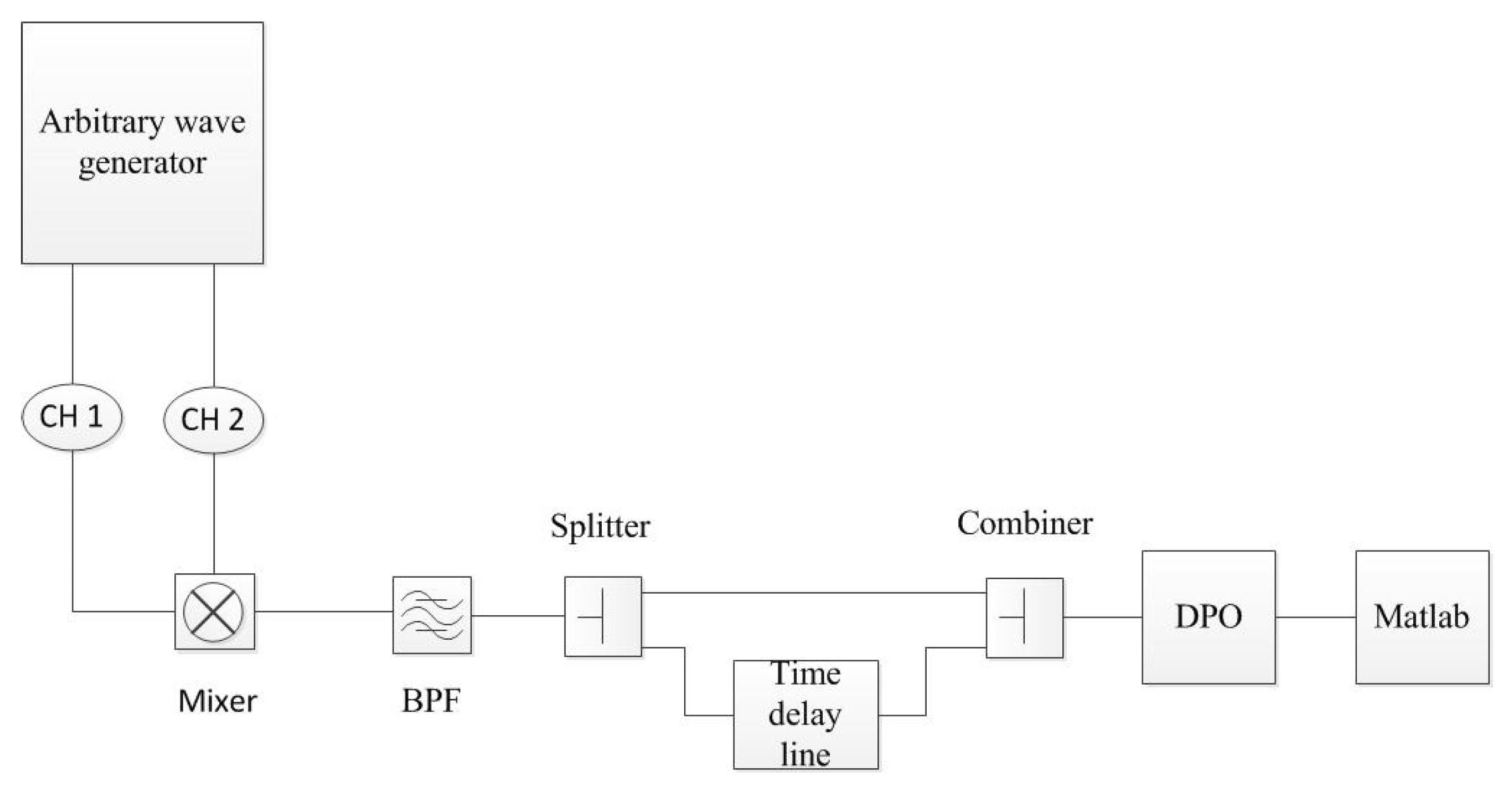
In many situations, such as atmosphere radiation measurement or vegetation radiation measurement, the spectrum of the measured signal remains unchanged during the measuring time, and the measured signal can be seen as the stationary signal. As mentioned in Section 2, the M(l)-C(s) arrangement slides across the input signal and only performs the Fourier transform of some parts of the input signal. Thus, the M(l)-C(s) arrangement is only suitable for the measurement of the stationary signal. In addition, the intermittent measurement of the M(l)-C(s) arrangement degrades the system’s sensitivity. A novel and simple CTS structure with only one M(l)-C(s) arrangement and a time delay line was developed for the measurement of the stationary signal as shown in Figure 3.

In Figure 3, the input signal is firstly mixed with the chirp signal to obtain the modulated intermediate frequency (IF) chirp signal. Then, after the amplifier, the modulated IF chirp signal is divided into two parts, which have a half period (10 µs) time delay between each other. Subsequently, the two parts are combined, filtered and compressed into pulses in time domain though the SAW filter. The time delay line guarantees a 100% duty cycle in the measurement. It is important to note that the output pulses from the structure in Figure 3 are different from the simple doubling of the output pulses from single M(l)-C(s) arrangement. The initial phases of the IF chirp signals and the noise are different before and after the time delay line. As the SAW filter is not sensitive to the initial phase, the IF chirp signals before and after the time delay line are both compressed into the same pulses (with a 10 µs time delay), while the noise is not compressed. Therefore, this novel CTS system based on one M(l)-C(s) arrangement has the same system sensitivity as the classical two-channel CTS system. Compared to the classical two-channel push-pull CTS system, this novel structure has fewer devices and reduced mass, which may have potential applications in the area of aviation.

3.2. FCS M-C Arrangement

Another novel frequency conversion single M(l)-C(s) arrangement was also developed for stationary signal measurement as shown in Figure 4.

In the FCS M-C arrangement, the input signal is firstly mixed with the chirp signal to obtain the modulated IF chirp signal, which is similar to the M(l)-C(s) arrangement. Then, the modulated IF chirp signal is split into two parts; one is firstly mixed with an up-and-down conversion mixer and then combined with another part. Subsequently, signals from the combiner are sent to the SAW filter for final pulse compression. The added up-and-down conversion mixer actually helps to collect the missing parts of the input signal in the M(l)-C(s) arrangement. Thus, the FCS M-C arrangement can deal with the entire part of the input signal and obtain a full duty cycle in the expander-compressor arrangement. There is a matching network in the FCS M-C arrangement, which takes the dispersion delay of the up-and-down conversion mixer into consideration. Usually, the dispersion delay of mixer is at a picosecond level, which is much smaller than the time interval of the output pulses in most CTS systems, and its effect can be ignored. The two band-pass filters in the FCS M-C arrangement are used to filter out spurious signals, and the passband width is equal to the working bandwidth of the SAW filter. The fixed frequency sent to the LO port of the up-and-down mixer is equal to the bandwidth of the convolution filter. Only considering the signal passing though the added up-and-down mixer in the FCS M-C arrangement, the output of the SAW filter can be written as:

$$S_2\left(t\right)={\displaystyle {\int }_{-\infty }^{+\infty }f\left(\tau \right)\cdot \cos \left(2\pi \mu T_o\tau \right)}\cdot C_1\left(\tau \right)\cdot H_0\left(t-\tau \right)d\tau$$

(11)

where $\cos \left(2\pi \mu T_o\tau \right)$ indicates the up-and-down mixer and $\mu T_0$ is a fixed input frequency at the LO port. Equation (11) can be further written as:

$$S_2\left(t\right)={\displaystyle \prod \left(\frac{t-t^{\prime }}{T^{″}}\right)}{\displaystyle {\int }_{-\infty }^{+\infty }{\widehat{f}}_1\left(\tau \right)}\cdot \cos \left({\omega }_1\tau -\pi \mu {\tau }^2+{\varphi }_1\right)\cdot \cos \left\{{\omega }_0(t-\tau )+\pi \mu {\left(t-\tau \right)}^2+{\varphi }_0\right\}d\tau$$

(12)

where

$${\widehat{f}}_1\left(\tau \right)=f\left(\tau \right){\displaystyle \prod \left(\frac{t-\tau -\frac{1}{2}{T}_0}{T_0}\right)}\cdot \cos \left(2\pi \mu T_0\tau \right)$$

(13)

Let $\mathsf{\Omega }={\omega }_0-{\omega }_1+2\pi \mu \left(t\pm T_0\right)$ and $x_1\left(\tau \right)=\widehat{f}\left(\tau \pm T_0\right)\cdot \exp \left[j\left({\omega }_{0}t+\pi \mu t^2+{\varphi }_0+{\varphi }_1\right)\right]$, Equation (13) can be rewritten as:

$$S_2\left(t\right)={\displaystyle \prod \left(\frac{t-t^{\prime }}{T^{″}}\right)}\left(X_1\left(\mathsf{\Omega }\right)+X_1^{\ast }\left(\mathsf{\Omega }\right)\right)$$

(14)

where $X_1\left(\mathsf{\Omega }\right)$ is Fourier transform of $x_1\left(t\right)$. Equation (14) indicates that the FCS M-C arrangement performs the Fourier transform of $\widehat{f}\left(t\pm T_0\right)$, which represents the previous and later parts of the input signal with a time interval of $T_0$. It can be seen that the added up-and-down mixer in the FCS M-C arrangement helps to obtain a full duty cycle in each period, which achieves a similar effect to the classical two-channel push-pull CTS system.

4. Simulation and Analysis

To validate the proposed two novel expander-compressor arrangements, three simulation models were built in Advanced Design System (ADS). One is based on the TDS M-C arrangement, and one is based on the FCS M-C arrangement. A model based on the classical two-channel push-pull CTS system was also built for comparison. The input signals were set to be several discrete cosine signals with identical amplitude. The expander chirp signal was generated by a voltage source in ADS. A s2p file was created to replace the SAW filter for pulse compression. The output pulses and the frequency resolution were measured and analyzed.

4.1. Simulation of the TDS M-C Arrangement

The input signals are four stationary discrete cosine signals with frequencies of 1.8 GHz, 1.9 GHz, 2.0 GHz and 2.1 GHz. The expander chirp signal has a bandwidth of 1.2 GHz and is centered at 3.1 GHz. The chirp rate is 60 MHz/µs and the time duration is 20 µs. The total simulation time was set to be 50 µs. Figure 5 shows the output pulses from the TDS M-C arrangement and the classical two-channel CTS. The different output pulses in the time domain represent the different input frequencies. It can be seen that the time interval of the output pulses is 1.667 µs, which corresponds to the 100 MHz frequency interval between the input frequencies considering the chirp rate of 60 MHz/µs. The time delay line in the TDS M-C arrangement helps to move the output pulses from one period to the nearby period acquiring a 100% duty cycle, which has the same effect as the other channel in the classical two-channel CTS structure. The amplitudes of the output pulses are a little different, and the maximum difference is between the pulses at m1 and m2, which is about 5 percent difference. This is mainly caused by the non-ideal mixer in the simulation, which has different conversion loss for the different input frequencies. As the phase response of the time delay line is random, the system sensitivity of the TDS M-C arrangement is the same as that of the classical two-channel CTS structure. Figure 6 shows the pulses at 13.34 µs from the classical two-channel CTS structure and the pulses at 23.34 µs from the TDS M-C arrangement. Both pulses have the shape of a sinc function, and the time widths of the pulses are the same, which virtually reflects the system’s frequency resolution.

4.2. Simulation of the FCS M-C Arrangement

Another set of parameters of input signals was used in the simulation of the FCS M-C arrangement. The input stationary signal is with four frequencies of 1.8 GHz, 1.85 GHz, 1.95 GHz and 2.15 GHz. The input signal to the LO port of the up-and-down conversion mixer is a cosine signal with a frequency of 600 MHz, which is equal to the bandwidth of the modulated IF chirp signal. The simulation results are shown in Figure 7. The time difference between the pulses appearing at m1 and m2 is 1.67 µs, which corresponds to the frequency difference (1 GHz) of the two input frequencies of 1.85 GHz and 1.95 GHz, considering the chirp rate of 60 MHz/µs. The amplitude difference comes from the conversion loss of the non-ideal mixer. It can be seen that there are three small pulses at the first 10 µs. These pulses result from the partial compression of the input frequencies of 1.85 GHz, 1.95 GHz and 2.15 GHz. This can be also explained by Equation (14). Figure 8 shows the output pulses appearing at 22.5 µs from the classical two-channel CTS structure and the FCS M-C arrangement. The amplitudes and time widths of the two pulses are almost the same, and this indicates that the frequency resolutions of the two methods are almost the same.

5. Experiment and Analysis

Two experiments were conducted to validate the TDS M-C arrangement and the FCS M-C arrangement individually. The expander chirp signal and the input signals were both generated from the arbitrary waveform generator (AWG). Limited by the processing difficulty and high manufacturing cost of the SAW filter, a s2p file was used as an alternative. The IF chirp signal was sampled and stored using a digital phosphor oscilloscope (DPO), and the final pulse compression was realized in MATLAB. The expander chirp signal ranges from 2.5 GHz to 3.7 GHz with a time duration of 20 µs. The input signals are four cosine signals with frequencies of 1.8 GHz, 1.9 GHz, 2.0 GHz and 2.1 GHz.

5.1. TDS M-C Arrangement Experiment

The experimental schematic diagram of the TDS M-C arrangement is shown in Figure 9. In the TDS M-C arrangement experiment, the expander chirp signal and the measured signals were both generated by AWG7082c (Tektronix, Beaverton, OR, USA). After the mixer and the band-pass filter, the IF chirp signal was then divided into two parts by a splitter. One was delayed for 10 µs and then combined with another part. The time delay line was a 10 µs fiber delay line with a bandwidth from 0.7 GHz to 1.3 GHz and a delay error less than 1%. The combined signal was then sampled and stored by the DPO. Subsequently, the digital IF chirp signal was sent to MATLAB for the final pulse compression.

The output pulses are shown in Figure 10. Due to the different conversion loss of the mixer, there are some differences between the amplitudes of the pulses in each period. The entire amplitudes of the pulses between 20 µs to 30 µs are slightly smaller than the pulses between 10 µs to 20 µs. This is due to the insertion loss of the time delay line, which is about 0.12 dB.

5.2. FCS M-C Arrangement Experiment

The experiment circuit for the FCS M-C arrangement is shown in Figure 11. The generation of the expander chirp signal, the measured frequencies and the modulated procedure to obtain the IF chirp signal were the same as those of the TDS M-C arrangement experiment. The main difference is that in the FCS M-C arrangement experiment, an up-and-down conversion mixer was used to replace the time delay line. The added up-and-down conversion mixer has a LO input with a fixed frequency of 600 MHz, which is equal to the bandwidth of the IF chirp signal. The output IF chirp signal was also sampled and stored by a DPO and then sent to MATLAB for the final pulse compression.

The final output pulses are shown in Figure 12. It can be seen that the amplitudes of pulses from the up-and-down conversion channel (channel 2) are much smaller than those from channel 1, and the power differences range from 10.4 dB to 11.8 dB. This is mainly caused by the conversion loss of mixer 2. The up-conversion loss and the down-conversion loss of mixer 2 are shown in Figure 13 and Figure 14. The average conversion loss of mixer 2 is about 9.3 dB, which is close to the power difference between the two channels. This fixed power difference due to the conversion loss of mixer 2 can be compensated in the later digital signal-processing procedure. Meanwhile, the insertion loss of the line, the splitter and the combiner also have a slight influence on the amplitude accuracy of the output pulses.

The full-width half-maximum (FWHM) [12] method was used to retrieve the spectral resolution of the TDS M-C arrangement and the FCS M-C arrangement. A high resolution sampling rate of 10 kHz was used to locate the maximum and the neighbor half maximum points from the output pulses. Then, the relative half-width half-maximum (HWHM) to the left and right could be measured. The average value of the left and right HWHM is the FWHM, which is the system’s spectral resolution. The calculated average FWHM widths of the two novel arrangements are shown in Figure 15. The average FWHM widths of the FCS M-C arrangement and the TDS M-C arrangement are about 91.5 kHz and 90.7 kHz, respectively. They are both close to the maximum achievable spectral resolution (88 kHz) of the M-C arrangement, which is defined by the compressor’s chirp length [12].

6. Conclusions

The M(l)-C(s) arrangement is a classical structure for pulse compression and spectral analysis of stationary signal. However, the system’s sensitivity is degraded when only using one single M-C arrangement for pulse compression. The classical two-channel push-pull CTS system with two M-C arrangements working alternately can improve the system’s sensitivity. The only challenge is the match between the two channels, especially the match between the two SAW filters, which affects the spectral performance. With the development of the FCS M-C arrangement and the TDS M-C arrangement, which only include one M-C arrangement, fewer devices are required, and the matching problem is avoided. The simulation and experimental test demonstrate that these two novel arrangements can achieve the same output pulses as the classical two-channel CTS structure and may have potential application in spaceborne spectroscopy.

References

1. Lawrence, M. Transformations in Optics; Wiley: New York, NY, USA, 1965. [Google Scholar]
2. Klauder, J.R.; Price, A.C.; Darlington, S.; Albersheim, W.J. The Theory and Design of Chirp Radars. Bell Syst. Tech. J. 2013, 39, 4. [Google Scholar] [CrossRef]
3. Williamson, R.C.; Smith, H.I. Large-time-bandwidth-product surface-wave pulse compressor employing reflective gratings. Electron. Lett. 1972, 8, 401–402. [Google Scholar] [CrossRef] [Green Version]
4. Morgan, D.P. Surface-Wave Devices for Signal Processing; Elsevier: Amsterdam, Netherlands, 1985. [Google Scholar]
5. Otto, O.W. Real-time Fourier transform with a surface-wave convolver. Electron. Lett. 1972, 8, 623–624. [Google Scholar] [CrossRef]
6. Hartogh, P.; Hartmann, G.K.; Heimesaat, G. The use of Chirp-transform-spectrometers for real time Fouriertransform of stochastic signals. Adm. Sci. Q. 1989, 21, 634–635. [Google Scholar]
7. Hartogh, P.; Hartmann, G.K. A high-resolution chirp transform spectrometer for microwave measurements. Meas. Sci. Technol. 1990, 1, 592. [Google Scholar] [CrossRef]
8. Li, X.Y. Development of RAC Devices Fabricated Using E-Beam Lithography for Chirp Transform Spectrometers. Ph.D. Thesis, Albert-Ludwigs-Universität Freiburg, Breisgau, Cermany, 2010. [Google Scholar]
9. Klein, B.; Philipp, S.D.; Güsten, R.; Krämer, I.; Samtleben, D. A new generation of spectrometers for radio astronomy: Fast Fourier Transform Spectrometer. In Millimeter and Submillimeter Detectors and Instrumentation for Astronomy III; SPIE—The International Society for Optical Engineering: Bellingham, WA, USA, 2006; Volume 6275. [Google Scholar]
10. Jack, M.; Grant, P.; Collins, J. The theory, design, and applications of surface acoustic wave Fourier-transform processors. Proc. IEEE 1980, 68, 450–468. [Google Scholar] [CrossRef]
11. Villanueva, G.L.; Hartogh, P.; Reindl, L.M. A digital dispersive matching network for SAW devices in chirp transform spectrometers. IEEE Trans. Microw. Theory Tech. 2006, 54, 1415–1424. [Google Scholar] [CrossRef]
12. Villanueva, G.L. The High Resolution Spectrometer for SOFIAGREAT: Instrumentation, Atmospheric Modeling and Observations. Ph.D. Thesis, Fac. Appl. Sci., Freiburg Univ.,, Freiburg, Germany, 2004. [Google Scholar]
13. Hartogh, P. High-resolution chirp transform spectrometer for middle atmospheric microwave sounding. In Satellite Remote Sensing of Clouds & the Atmosphere II; International Society for Optics and Photonics: Bellingham, WA, USA, 1998. [Google Scholar]
14. Seele, C.; Hartogh, P. Water vapor of the polar middle atmosphere: Annual variation and summer mesosphere Conditions as observed by ground-based microwave spectroscopy. Geophys. Res. Lett. 1999, 26, 1517–1520. [Google Scholar] [CrossRef]
15. Hofstadter, D.; Hartogh, P.; McMullin, J.P.; Martin, R.N.; Jarchow, C.; Peters, W. A search for variability in the HCN to H2CO ratio in comet Hale-Bopp. Earth Moon Planets 1997, 78, 53–61. [Google Scholar] [CrossRef]
16. Hartogh, P.; Fujisada, H. Present and future chirp transform spectrometers for microwave remote sensing. IEEE Trans. Microw. Theory Tech. 1997, 3221, 328–339. [Google Scholar]
17. Villanueva, G.L.; Hartogh, P.; Reindl, L. Microwave technologies on SOFIA’s high resolution spectrometer. In Proceedings of the 33rd European Microwave Conference, Munich, Germany, 7 October 2003; pp. 547–550. [Google Scholar]
Figure 1. M(l)-C(s) chirp transform processor arrangement.
Electronics 10 00065 g001
Figure 2. Simplified structure of the two-channel push-pull chirp transform spectrometer (CTS) system based on two M(l)-C(s) arrangements.
Electronics 10 00065 g002
Figure 3. The structure of the time delay single M(l)-C(s) (TDS M-C) arrangement.
Electronics 10 00065 g003
Figure 4. The structure of the frequency conversion single M(l)-C(s) (FCS M-C) arrangement.
Electronics 10 00065 g004
Figure 5. Output pulses of the four input frequencies. (a) is compressed by the classical two-channel chirp transform spectrometer (CTS) structure; (b) is compressed by the TDS M-C arrangement.
Electronics 10 00065 g005
Figure 6. Single pulse shape of the input frequency of 1.9 GHz. (a) is the pulse appearing at 13.338 µs from the classical two-channel CTS structure; (b) is the pulse appearing at the next period (23.338 µs) from the TDS M-C arrangement.
Electronics 10 00065 g006
Figure 7. Output pulses of the four input frequencies. (a) is compressed by the classical two-channel CTS structure; (b) is compressed by the FCS M-C arrangement.
Electronics 10 00065 g007
Figure 8. Single pulse appearing at 22.5 µs compressed from the input frequency of 1.85 GHz. (a) is the pulse compressed by the classical two-channel CTS structure; (b) is the pulse compressed by the FCS M-C arrangement.
Electronics 10 00065 g008
Figure 9. Experimental schematic diagram of the TDS M-C arrangement.
Electronics 10 00065 g009
Figure 10. Output pulses of the TDS M-C arrangement.
Electronics 10 00065 g010
Figure 11. Experiment circuit for the FCS M-C arrangement.
Electronics 10 00065 g011
Figure 12. Output pulses of the FCS M-C arrangement.
Electronics 10 00065 g012
Figure 13. The measured S21 of mixer 2 (up-conversion).
Electronics 10 00065 g013
Figure 14. The measured S21 of mixer 2 (down-conversion).
Electronics 10 00065 g014
Figure 15. The calculated average full-width half-maximum (FWHM) widths of the FCS M-C arrangement and the TDS M-C arrangement.
Electronics 10 00065 g015
Publisher’s Note: MDPI stays neutral with regard to jurisdictional claims in published maps and institutional affiliations.