Abstract
Evolutionary fuzzers generally work well with typical software programs because of their simple algorithm. However, there is a limitation that some paths with complex constraints cannot be tested even after long execution. Fuzzers based on concolic execution have emerged to address this issue. The concolic execution fuzzers also have limitations in scalability. Recently, the gradient-based fuzzers that use a gradient to mutate inputs have been introduced. Gradient-based fuzzers can be applied to real-world programs and achieve high code coverage. However, there is a problem that the existing gradient-based fuzzers require heavyweight analysis or sufficient learning time. In this paper, we propose a new type of gradient-based fuzzer, MaxAFL, to overcome the limitations of existing gradient-based fuzzers. Our approach constructs an objective function through fine-grained static analysis. After constructing a well-made objective function, we can apply the gradient-based optimization algorithm. We use a modified gradient-descent algorithm to minimize our objective function and propose some probabilistic techniques to escape local optimum. We introduce an adaptive objective function which aims to explore various paths in the program. We implemented MaxAFL based on the original AFL. MaxAFL achieved increase of code coverage per time compared with three other fuzzers in six open-source Linux binaries. We also measured cumulative code coverage per total execution, and MaxAFL outperformed the other fuzzers in this metric. Finally, MaxAFL can also find more bugs than the other fuzzers.
1. Introduction
Software vulnerabilities can be a tremendous threat to computer security. Therefore, many companies and security researchers have tried to find software vulnerabilities both manually and automatically. Finding vulnerabilities manually requires highly educated engineers, so various types of automatic methods were developed by researchers. Since Miller et al. [1] introduced fuzzing, it has become the best technique to find software vulnerabilities automatically. A fuzzer executes a program repeatedly with generated inputs to cause abnormal behavior of the software program. However, due to the simple algorithm, fuzzers had a problem with efficiency. Consequently, many researchers have tried to increase the efficiency of fuzzing, resulting in various algorithms.
The most representative fuzzing algorithm is an evolutionary fuzzer, which is based on the evolutionary algorithm, such as AFL [2]. The ultimate goal of fuzzing is to cause crashes in the Program Under Testing (PUT). However, the occurrence of a crash is very rare. Therefore, many fuzzers set their goal to maximize cumulative code coverage. Evolutionary fuzzers compute fitness scores using code coverage and maintain a queue of meaningful input values based on the fitness score. With the inputs in a queue, they select one input from the queue and mutate it to explore new paths.
Evolutionary fuzzers perform well in many types of programs, because of their simplicity. However, the biggest problem of evolutionary fuzzers is that they do not care about the internal logic of the program and structure of inputs. Therefore, almost no evolutionary fuzzer can reach hard-to-explore paths in the program. This is crucial in performance because many software crashes occur in hard-to-explore paths. The evolutionary fuzzers like AFL [2] use only simple mutation (e.g., bitflipping, arithmetic operation) as a deterministic stage. It is absolutely slow and inefficient because they cannot infer the mutation direction. Therefore, if the seed input of AFL increases, the deterministic mutation stage of AFL becomes extremely slow. Some previous works like AFLFast [3] and FairFuzz [4] tried to mitigate these problems by improving algorithms of AFL, however, they could not solve the limitations perfectly.
In order to test hard-to-explore branches, several methods have been proposed. The most common method is the concolic execution which can solve complex path constraints using SMT solver. Some fuzzers such as Driller [5] and QSYM [6], used concolic execution to reach various branches in the fuzzing process. Although concolic execution has the advantage to examine hard-to-explore paths, there is a serious performance problem due to a path explosion. This time complexity issue is a critical limitation of concolic execution fuzzers, so they cannot scale out to real-world programs.
Fuzzers such as Angora [7] and NEUZZ [8] used a gradient-based optimization to explore paths. To apply a gradient-based optimization algorithm to the fuzzing problem, Angora created a simple objective function using branch constraints, and NEUZZ modeled the program’s branching behavior using a surrogate neural network. Both fuzzers outperformed the traditional evolutionary fuzzers. Although gradient-based fuzzers show superior performance, there are some drawbacks. Angora requires heavyweight static and dynamic analysis before and during fuzzing. The analysis processes, such as type inference and taint analysis, need considerable time when applied to large binaries. NEUZZ must train a deep neural network before applying to fuzzing. If the size of the fuzzing binary is increased, training time might be also increased drastically. In addition, they do not care about the problem of local optima, therefore, in many cases, these types of fuzzers cannot find global optima.
To overcome the above limitations, we present a new fuzzer called MaxAFL. We modified the deterministic stage of AFL with a new gradient-based mutation algorithm. Firstly, we calculate Maximum Expectation of Instruction Count (MEIC) to determine the best path to explore during fuzzing. After calculating MEIC, we generate an objective function that can be used to maximize cumulative code coverage using MEIC and branch information. MaxAFL uses a gradient-based optimization to minimize the objective function. While minimizing the objective function, we can find better inputs for fuzzing. After enough time of fuzzing, the objective function is modified little by little to focus on a path that has never been explored. Additionally, in order to solve the problem of local optimum, we add some randomness in the optimization process through a simple bitflipping and normal sampling.
We implemented MaxAFL based on AFL 2.56b and LLVM 7.0.1. We compared MaxAFL with the original AFL [2], AFLFast [3] and FairFuzz [4] on six Linux binaries. We focus on three different metrics to evaluate performance: code coverage per a constant time, code coverage per a total execution, and the number of unique crashes. As a result, MaxAFL showed improved performance compared with the other fuzzers.
Contributions: Our contributions are as follows:
- We calculate MEIC to guide the direction of fuzzing through lightweight static analysis.
- We generate an objective function using MEIC and branch information. In this way, we can convert the fuzzing problem to an optimization problem, effectively.
- Based on the objective function we created, we use a gradient-based optimization to find efficient input for fuzzing. In this process, some probabilistic mutations are introduced to solve the problem of local optima. To explore various paths, MaxAFL continually updates the objective function.
- We implemented MaxAFL by changing only the deterministic mutation stage of AFL.
- We tested our fuzzer on six Linux binaries and compared the result with AFL, AFLFast, and FairFuzz. MaxAFL gains code coverage increment per time. It also shows an improvement of code coverage per total executions. When running MaxAFL in LAVA-M dataset, we found 47 more bugs compared with the other fuzzers.
2. Background
2.1. Fuzzing
Fuzzing is a software testing technique that finds bugs in programs. It passes various inputs to the target program to cause abnormal behavior of the program. Since the primary goal of fuzzing is to find more crashes, the most intuitive performance metric is the number of crashes found per time. However, the crashes occur very rarely, so most existing fuzzers are designed to maximize code coverage. Intuitively, increasing the code coverage enables testing more paths in the program, so we can increase the probability to find crashes. Many unseen crashes occur in deep code paths, because developers usually do not care about the codes that are not executed frequently. Consequently, the key of fuzzing algorithms is to find the input that maximizes the code coverage.
Typical fuzzers can be divided into two categories: mutation-based fuzzer and generation-based fuzzer. Mutation-based fuzzers generate new inputs by mutating seed inputs. These fuzzers show various performances depending on the mutation action. The most common mutation actions are bit-flip, byte-flip, insert dictionary, and so on. Mutation-based fuzzers are easy to implement and have the advantage that they can be used generally in various types of binary inputs. However, in the case of programs that take formatted files as input, mutation-based fuzzers show extremely low performance, because of parsing errors. Generation-based fuzzers are widely used in fuzzing programs that use formatted inputs (e.g., PDF, XML, source code, etc.). They analyze and model the input format, and then generate new test cases based on the model. Generation-based fuzzers can make structured inputs that may be accepted in the program, so they can decrease the occurrence of parsing errors. However, they must create a sophisticated model of input using appropriate algorithms.
Mutation-based fuzzers have been upgraded using various algorithms for a long time. They have largely developed with three big branches: Evolutionary fuzzer, Concolic execution fuzzer, Gradient-based fuzzer.
2.1.1. Evolutionary Fuzzer
The most common mutation-based fuzzer is the evolutionary fuzzer. It is based on an evolutionary algorithm that generates new populations of inputs using seed inputs. They mutate inputs from the initial seeds and collect interesting inputs which gain high code coverage or explore new paths. Because they use code coverage to calculate a score of the newly generated inputs, they are also called coverage-based greybox fuzzers [3]. These fuzzers perform very well on a wide range of targets due to fast execution speeds, despite the simple random mutation algorithms. The most famous evolutionary fuzzer is AFL [2]. Mutation stages of AFL consist of two main stages: the deterministic stage and non-deterministic stage.
In the deterministic stage of AFL, AFL selects various mutation actions in a fixed order. The mutation actions used in the deterministic stage include bit and byte flipping, set interesting values (replace bytes with pre-defined interesting values), simple arithmetic operations, etc. However, these mutation actions can slow down the overall fuzzing process, because they do not consider the direction of mutation. The number of mutations in the deterministic stage increases drastically in proportion to the seed input size, because it mutates almost every byte of the input. Therefore, if there is a large size of seed input, the deterministic stage of AFL takes a long time.
In the non-deterministic stage (havoc stage) of AFL, various mutation actions are chosen with equal probability. The mutation actions in the non-deterministic stage are similar to mutation actions of the deterministic stage, however, they select which byte to mutate and a parameter of mutation action (e.g., Integer K that is used in arithmetic addition or subtraction). Moreover, the total number of mutations in the non-deterministic stage is also determined randomly.
AFL uses minimal dynamic or static binary instrumentation to measure code coverage, resulting in fast fuzzing speeds. In addition, it offers a variety of internal functions such as trimming to remove non-critical parts of the input and calibration to precisely analyze the input. Böhme et al. [3] defined the overall algorithm of the evolutionary fuzzer (coverage-based greybox fuzzer), including AFL, as described in Algorithm 1.
| Algorithm 1 Evolutionary fuzzing (Coverage-based greybox fuzzer) [3] |
|
Detailed descriptions of each stage of Algorithm 1 are as follows.
- chooseNext : chooses next seed input s from seed corpus S to mutate.
- assignEnergy : decides how many times to mutate the seed input s.
- mutate_input : mutates seed input s using mutation algorithm and generates new input .
- isInteresting : determines whether newly generated input is significant or not.
2.1.2. Concolic Execution Fuzzer
In the case of hard-to-explore paths, such as Magic-byte checking code, it is almost impossible to explore these paths with a random mutation. In order to overcome this limitation, a new type of fuzzer was proposed using concolic execution. Concolic execution is a mixed technique that performs symbolic execution and concrete execution. Symbolic execution can solve many constraints on a specific path with the SMT solver. However, the symbolic execution is horribly inefficient in some cases such as loop code. Although symbolic execution has problems such as path-explosion and slow execution speed, the concolic execution mitigates this problem by performing concrete execution as much as possible and using symbolic execution only when it is necessary. Concolic execution fuzzers can explore some deep nested branches, but it cannot be scaled out to real-world programs that have complicated program logic due to path explosion.
2.1.3. Gradient-Based Fuzzer
Although the concolic execution has explored the deep nested branches, there is a critical limitation that it cannot scale-out to real-world programs. To bypass this limitation, new fuzzers have recently been introduced using gradient-based optimization. This type of fuzzer sets up an objective function to solve path constraints and apply the gradient-based optimization algorithm to minimize or maximize the objective function. While optimizing an objective function, we can explore the target path with high probability.
2.2. Program Analysis and Code Coverage
In order to test the overall source code, it is necessary to analyze the structure and behavior of the program. There are many ways to model programs, but the most famous model is probably the graph model.
2.2.1. Control Flow Graph and Call Graph
The best way to understand the execution flow of programs is to construct the Control Flow Graph (CFG) and the Call Graph. The CFG is a graph that shows the execution flow of the program in one function. The basic unit of CFG is the basic block which is a straight-line code sequence with no branches. Each basic block becomes a node of CFG and edges represent the execution order between the basic blocks. We can generate the control flow graph quickly using simple static analysis. The call graph is a graph that shows the call relations among the internal functions of the program and can be used to determine the relations between the functions. If a function A calls a function B, the edge from A to B is added to the call graph. These two graphs are useful in fuzzing because we can know execution flows very accurately.
2.2.2. Code Coverage
Code coverage is a metric to evaluate how many parts of a program have been tested in software testing. In general, the higher the code coverage, the better the testing result because it means that the testing method can execute large part of the program. Code coverage is used in many software testing techniques, but it is particularly important in the fuzzing process. The purpose of fuzzing is causing an abnormal behavior (Crash) of the program, however since such behaviors occur very rarely, code coverage is used for calculating the efficiency of the fuzzing process. Representatively, the coverage-based greybox fuzzer, mentioned before, uses code coverage to determine how good the current input value is.
There are various types of code coverage. Typical code coverages are as follows [9].
- Instruction coverage: has each instruction in program been executed?
- Line coverage: has each line of code in the program been executed?
- Basic block coverage: has each basic block in the program been executed?
- Branch coverage: has each branch in the program been executed with both true and false conditions?
- Condition coverage: has each boolean sub-expression been evaluated both to true and false?
- Edge coverage: has each edge in the CFG of program been executed?
- Function (method) coverage: has each function (or method) in the program been called?
The code coverages used in most fuzzing researches do not deviate much from the coverage presented above [10]. In this paper, line coverage is mainly used as a coverage metric.
2.3. Gradient-Based Optimization
Methods of mathematical optimization are old methods widely used in various fields like mathematics, computer science, and economics. The simplest form of an optimization problem is to find an input x that maximizes or minimizes a given function f. This can be simply expressed by
where S is the domain of input x (e.g., in continuous optimization) and is an objective function. Among these, the gradient-based optimization is an algorithm that finds the direction of optimization by calculating the gradient of the objective function. The general gradient-based optimization is described in Algorithm 2.
| Algorithm 2 Gradient-based optimization for objective function f |
|
2.3.1. Gradient Descent
The gradient descent is the most popular gradient-based optimization algorithm that uses the first derivative of the objective function to find the optimal value. While finding the minimum value, the gradient descent changes the input in a negative direction of the gradient at the current point. While finding the maximum value, it modifies the input value in a positive direction of the gradient. With the multivariate function and the current input , the gradient descent repeats the following calculation to find the optimal value.
where represents a learning rate and the algorithm terminates when x finally converges.
2.3.2. Subgradient Method
Since gradient descent needs the derivative of , has to be differentiable. However, in many cases, the objective function is not differentiable, so we should use another value for finding the direction. Subgradient can be generally a good solution. Subgradient generalizes the derivative to convex functions which are not necessarily differentiable. The rigorous mathematical definition of the subgradient of the function is as follows:
where S is the domain of f. Figure 1 shows a graphical example of the subgradient of non-differential function . We can use subgradient as the direction of optimization instead of a gradient of , in the case of non-differential function. Figure 1 shows elementary examples of subgradient of arbitrary function f.
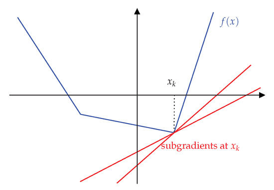
Figure 1.
Example of subgradient of an arbitrary function f at . The blue line is a graph of the function f and the red lines are possible candidates of subgradient.
2.3.3. Numerical Differentiation
To calculate the gradient used in the gradient-based optimization, there are three types of methods: automatic method, symbolic method, and numerical methods. Automatic differentiation and symbolic differentiation can be used when the formula of the objective function is known. These methods are faster than the numerical methods, but these are used only in special cases due to rigorous conditions of use. For example, in neural networks, we can calculate the gradient of loss function using the back-propagation algorithm to train a neural network, because the structure of the network is known and the loss function is differentiable [11].
If the objective function is composed of non-differentiable equations, we have to use the numerical differentiation. This method calculates an estimation of the gradient (or subgradient) by simply changing the x value little by little and measuring the changes of function output. Depending on whether we change the value of x in the positive or negative direction, it is called ’forward divided differences’ and ’backward divided differences’, respectively. The most commonly used numerical gradient value is the ’symmetric difference’ that is calculated by changing x both in the positive and negative directions. Symmetric difference is more accurate than one-sided estimations. The expression of symmetric difference is defined by
The numerical differentiation is slower than the others in practice, but we can use this method in general, even if the function is extremely sophisticated.
2.3.4. Gradient Clipping
The gradient clipping is a technique to prevent exploding gradients. It is usually used in deep neural networks because of exploding and vanishing gradients [11]. This technique can help the gradient descent process by limiting the range of the gradient. The simple algorithm of gradient clipping is described in Algorithm 3.
| Algorithm 3 Simple gradient clipping |
|
2.3.5. Local Optimum and Global Optimum
One of the problems of gradient-based optimization is getting stuck in a local optimum. Local optimum means a solution that is optimal within nearby candidates. In contrast, global optimum means that the solution is optimal among all possible solutions. Of course, we want to find global optimum, but if we just follow the gradient of the objective function, it can get stuck in local optimum with high probability.
We can fix this problem using some stochastic methods. Simulated annealing [12,13] can find global optimum by moving to some neighboring state with an acceptance probability. Even simple algorithms like random restart [14] can help find a global optimum.
3. Related Work
3.1. Evolutionary Fuzzer
The evolutionary fuzzer is a simple fuzzer based on an evolutionary algorithm. Starting with initial seed inputs, they mutate these seed inputs and keep the input queue with better inputs to test the program. They have their own fitness function which is used to prioritize the test cases. Most of these fuzzers use code coverage as a fitness function, so they are also called coverage-guided fuzzer.
The most famous evolutionary fuzzer is AFL [2]. AFL can efficiently test various programs with a simple mutation algorithm. Because AFL relies on a simple algorithm and basic instrumentation, it has great scalability. However, there is an inefficiency in the deterministic mutation stage, we fixed this problem using the gradient-based mutation. LibFuzzer [15] of LLVM Framework [16] and Honggfuzz [17] are also good examples of simple evolutionary fuzzer. AFLGo [18], AFLFast [3], FairFuzz [4], AFLSmart [19] are AFL-based fuzzers, which improve the fitness function, mutation actions, and power scheduling algorithm in the original AFL to improve the performance. CollAFL [20] has led to improved performance by developing a new coverage measurement method.
3.2. Concolic Execution Fuzzer
The symbolic execution analyzes the program by replacing the constraints on a certain path with symbolic values to search hard-to-explore paths. The path constraints information that is obtained in this way can be efficiently solved using the SMT solver like Z3 [21]. KLEE [22] is a representative symbolic execution framework. However, symbolic execution has poor scalability due to the path explosion problem. Concolic execution mitigates this issue by mixing the symbolic execution and concrete execution.
The concolic execution fuzzer is a fuzzer that efficiently searches for hard-to-explore path using the concolic execution engine. SAGE [23,24] and DART [25] applied the concolic execution engine to the fuzzer to generate appropriate inputs. Dowser [26] utilized static and dynamic analysis to minimize the symbolic execution due to the scalability issue. Driller [5] limited the symbolic execution only when the fuzzer cannot explore a certain path, thereby mitigating the path explosion. QSYM [6] introduced dynamic binary translation that can make the symbolic execution faster and more scalable than before. DigFuzz [27] categorizes the types of the concolic execution into “demand launch” and “optimal switch” and proposed a novel strategy called “discriminative dispatch”. By using the Monte Carlo-based path prioritization algorithm, they increased the efficiency of the concolic execution. Eclipser [28] proposed a grey-box concolic testing that does not depend on the SMT solver and only proceeds lightweight instrumentation.
Fuzzers using the concolic execution are being actively studied, but there is no way to completely solve the fundamental problem, path explosion. In addition, while almost all concolic execution fuzzers perform path search for a specific path, our approach can automatically set the search target during the optimization process.
3.3. Gradient-Based Fuzzer
Gradient-based fuzzers use a gradient of an objective function with respect to an input to mutate input, reasonably. Angora [7] searches paths using taint analysis, type and shape inference. Angora uses dynamic taint analysis which is a heavy analysis process. However, in our approach, only simple static analysis in the compile process is necessary. NEUZZ [8] utilizes a surrogate neural network that simulates the program branch behaviors for fuzzing. The neural network has to be sufficiently learned to predict the program behavior, and the gradient is efficiently calculated and used in the mutation process. However, NEUZZ has a limitation that it requires a sufficient learning time. Matryoshaka [29] identified control flow-dependent statements and taint flow-dependent statements to explore deeply nested paths. After then, based on the previous information, they solved the path constraints by using the gradient descent algorithm.
4. Machine Learning-Based Fuzzer
Recently, solving fuzzing problem based on machine learning have been continuously proposed. The aforementioned NEUZZ [8] is an example of applying a deep neural network for fuzzing. RLFuzz [30], FuzzerGym [31] are examples of applying a reinforcement learning, which has recently received increased interest, for fuzzing. These two fuzzers transform the fuzzing problem into a Markov Decision Process (MDP) form by defining a state, action, and reward and use the DQN algorithm to mutate the inputs. Rajpal et al. [32] learn the input format of a target program with a neural network to improve the performance of fuzzing. Learn&Fuzz [33] improves fuzzing performance by learning PDF structure using an LSTM model.
5. Proposed Approach
5.1. Overview
To overcome the limitations of existing fuzzers, we designed a following new approach which mainly consists of three parts: obtaining Maximum Expectation of Instruction Count (MEIC) through static analysis, generating the objective function to apply the gradient-based optimization, and fuzzing to minimize the objective function. The optimization algorithm consists of gradient descent for efficient path search and probabilistic method to search for various paths and avoid local optimum. We modify the objective function in the fuzzing process in order to explore the unexplored paths. Figure 2 shows the entire architecture of MaxAFL.
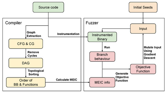
Figure 2.
Overview of MaxAFL. MaxAFL consists of two main component: Compiler and Fuzzer. Compiler performs static analysis for calculating MEIC and binary instrumentation. Fuzzer executes instrumented binary repeatedly using gradient-based mutation.
5.2. Motivating Example
We show a simple example code in Figure 3 to emphasize the effectiveness of our approach.
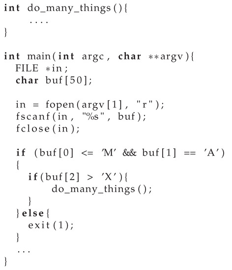
Figure 3.
Motivating example of our approach. do_many_ things() is a user-defined function with large source code.
In this example, the do_many_things() function consists of a lot of code lines. Therefore, we need to guide the execution flow to the do_many_things() function during the fuzzing process. In typical fuzzers like AFL, this path is difficult to explore due to two reasons. Firstly, at the beginning of fuzzing, we do not know which path is better to explore a large amount of code. Secondly, the constraints of the path are complicated, so the random mutation algorithm cannot find an appropriate input to test a certain path. In our example, to test do_many_things() function, we have to pass if statements at line 13 and line 15.
However, in our approach, we can figure out which branch is better at every basic block, so we can determine which path is better to test. After that, we set up the objective function to induce execution flow to the targeted path and find new inputs using gradient-based optimization.
5.3. Maximum Expectation of Instruction Count
To generate the input that maximizes code coverage, we infer the importance of every path by calculating the Maximum Expectation of Instruction Count (MEIC) for each basic block. MEIC is the maximum number of instructions that can be tested when we execute a specific basic block. If the control flow is always directed to the basic block which has bigger MEIC at every branch, simply in the best case, the instruction can be executed as much as MEIC. The calculated MEIC plays a key role in generating the objective function for further optimization.
Lightweight static analysis is required to calculate the MEIC. First, we should extract the program’s call graph and control flow graph to earn knowledge about execution flow. The MEIC of the current basic block can be calculated using their successor basic blocks and called functions in the current basic block. Accordingly, we have to figure out the order of every basic block in the target program. We have to know the calling orders of functions to determine which functions should be processed. Topological sorting is a useful algorithm to determine the order of nodes in the graph. Therefore, we execute topological sorting in the call graph to find the execution order from an entry function to an exit function.
After acquiring the execution order of functions, we can calculate the MEIC of each basic block by referring to the CFG of function. Since we need to figure out the execution order among the basic blocks inside the function, we also perform topological sorting in CFG. Note that topological sorting only works for a directed acyclic graph (DAG). Therefore, it is necessary to remove the cycles of the CFG caused by a loop before applying topological sorting. Hence, we obtain the information of loops and remove the backedges which direct to the previous basic block. In fuzzing, exploring a unique path is more important, so by removing that backedge, the instructions inside the loop are counted only once, no matter how many times they are executed. In addition, some programs may use the goto statement, therefore additional cycles can be detected. In this case, the cycle is detected and removed based on a simple depth-first search (DFS) algorithm. After removing all cycles, topological sorting is performed in the control flow graph and acquiring the order of basic blocks is finished. The MEIC can be calculated in order from the exit nodes to the entry node of CFG. Figure 4 demonstrates the process of calculating MEIC in one CFG.
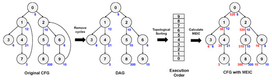
Figure 4.
Overview process of calculating Maximum Expectation of Instruction Count (MEIC). The blue number (number at the right side of each node) shows the instruction count of the basic block and the red number (number at the left side of each node) shows MEIC of the basic block.
If some functions are called in a basic block, we add MEIC of the called function to MEIC of the basic block. We only consider user-defined functions, because our goal is maximizing the code coverage of the user program. Since we figured out the calling order of each function, by calculating MEIC of function in reverse of calling order, we already know the MEIC of called functions at that time.
Now, we can calculate the MEIC of every basic block using the MEIC of successor basic blocks and the instruction count of the current basic blocks. Algorithm 4 is a procedure that describes the process of calculating MEIC after applying cycle elimination and topological sorting.
| Algorithm 4 Calculate MEIC of the program |
|
Figure 5 is an example of our process from CFG extraction to MEIC calculation that is applied to the motivating example in Figure 3. Figure 5a is the original CFG obtained using the LLVM framework, and the instructions of the program are described in each basic block. The instruction counts of each basic block can be simply calculated by counting the number of instructions. The calculated instruction count is represented by a blue number to the right of each basic block. The instruction which is marked with a green square is a call instruction that calls user-defined function do_many_things(). This call instruction should be considered when calculating MEIC later.
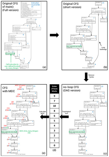
Figure 5.
The overall process for calculating MEIC of main() function in motivating example. (a) Original CFG of main() (full version); (b) Original CFG (short version); (c) no-loop CFG (DAG version); (d) Order of basic blocks; (e) CFG with MEIC.
Figure 5b is a short version of CFG without unnecessary instructions for explaining. As you can see in Figure 5b, there is one backedge created by the for statement in the main() function. it will be deleted for the next step.
Figure 5c is the CFG without the loop backedge. As mentioned earlier, in order to run the topological sorting, we should make DAG version of CFG.
Figure 5d is a table that is showing the result of topological sorting. The numbers in the table are the ids of basic blocks. From the top to the bottom, we can calculate MEIC of the basic block sequentially.
Finally, Figure 5e is a figure that is shows the MEIC of each basic block and the MEIC of the main() function. The MEIC of each basic block is described as the red number on the left side of the basic block. The MEIC of the main() function is defined as the MEIC of the entry basic block of the function. In the process of calculating the MEIC of basic block 5, the MEIC of the do_many_things() function must be added to MEIC of basic block 5, because there is a call instruction to do_many_things() function. In this example, for convenience, the MEIC of the do_many_things() function is arbitrarily set to 250.
5.4. Objective Function
To convert the fuzzing problem into an optimization problem, we create an objective function that can be used to maximize code coverage. Intuitively, because our goal is to maximize code coverage, we can use code coverage as an objective function, but there is a big problem. The distribution of code coverage in input space X is not continuous and smooth because it only depends on the execution flow in the program. Even if the input value x changes, the execution flow can be changed only at certain values, so in most cases, the gradient might be zero and the function is not continuous. For example, in the program of Figure 3, when buf[3] is ‘Z’, the numerical gradient of the code coverage with respect to buf[3] is zero and we cannot find the direction of the mutation.
To overcome this problem, we designed a new objective function to be as continuous as possible and to have a gradient at every point. In addition, to achieve the fundamental goal which is maximizing code coverage, the objective function is designed using the previously calculated MEIC. We always guide the control flow to a basic block with a higher MEIC at every branch within the program. To derive this branch behavior, we analyze the CMP instructions of the branch and MEIC of child basic blocks to generate the objective function.
Firstly, we calculate the branch variable v for every branch instruction. A branch variable is a variable that determines the control flow of a specific branch. It is defined as the difference between both variables of CMP instruction. For example, in the case of the conditional statement on line 15 in Figure 3, the branch variable is calculated as . In the case of an equal compare instruction (equal and not equal), the branch variable is defined in the same way.
After calculating the branch variable as above, the branch cost can be computed based on the MEIC of the next basic blocks and branch variable. Branch cost is based on simple intuition. If control flow goes to the wrong basic block, we treat it as a loss like a general loss in machine learning. Of course, if control flow goes to the right basic block, the cost will be zero. We defined the coefficient of the cost using the difference between MEIC of successor basic blocks, to prioritize important branches in an objective function. In addition, the branch variable is not used directly, because the range of the branch variable is too wide. For example, in the case of integer compare instruction, branch variable can be an integer between 0 and in x86 architecture. Of course, in x64 architecture, branch variable varies between 0 and . Furthermore, in the case of floating-point number comparison, there is no exact range of branch variable. Therefore, we not only limit the range of branch cost but also make it easier to converge using a sigmoid function as Equation (4).
where is a set of hyperparameters. The entire algorithm to calculate the branch cost is described as Algorithm 5.
Note that, through a simple compiler optimization, we made every basic block has only two child basic blocks. The complete objective function J consists of the sum of branch costs of all basic blocks that are executed at the current execution.
| Algorithm 5 Calculating branch cost |
|
5.5. Optimization Using Gradient Descent
For the purpose of generating efficient inputs, we minimize the objective function with the gradient descent algorithm. In this case, an input is divided into bytes and one byte is treated as one dimension. Therefore, each byte can have an integer value from 0 to 255 during the optimization process and rotates the value when overflow or underflow occurs (ex. 255 + 1 = 0, 0 − 1 = 255).
5.5.1. Estimate Subgradient
To perform gradient-based optimization, we need to estimate the gradient of the objective function J at the current input x. Our objective function is not perfectly continuous and smooth, so instead of a rigorous gradient, we use the subgradient of the function. Because our objective function is determined by the branch-behavior inside the program, we cannot represent it as a precise equation. So, in this case, we have to use a numerical method to calculate the subgradient. Simply, we obtain a subgradient with respect to input byte by calculating symmetric difference as Equation (3).
5.5.2. Mutate Input Using Subgradient
After approximating subgradient of J, we can generate a new input using the subgradient. Subgradient is a direction of mutation, so we only need to determine the learning rate in Equation (1). There are plenty of ways to decide , but we simply fix an initial learning rate and decrease using a decreasing rate like .
In the gradient descent process, we treat every byte as one dimension of a real number. However, bytes of real input must be an integer value between 0 and 255, so we round off every byte of x to convert input before passing it to the target program.
5.5.3. Gradient Clipping
One of the problems in the gradient descent is that x has changed so much and it jumps to an unintended position. This problem occurs because the learning rate is set too big or the search space is shaped like a waterfall and, consequently, the gradient is too big. However, if the learning rate is set too small, there is a disadvantage that the convergence time becomes too large which is a critical problem in the fuzzing process. In particular, in the case of our objective function, there are locations that cause gradient exploding and spaces that have very small gradients, so it is impossible to decrease the learning rate. Therefore, we solved this problem using the gradient clipping technique. As we briefly explained earlier in Algorithm 3, the gradient clipping is a simple method to reduce the gradient to a certain range when it is larger than a certain threshold. We conducted many experiments to set the threshold and figured out the best threshold to be 200 based on empirical evidence.
5.5.4. Termination Criteria
If x converges to local optima, the gradient descent will trivially terminate, because the goal of the algorithm is achieved. However, in many cases, x cannot converge and move around the local optima due to some problems. Even if we know that it will converge in the future, convergence time must be small enough because of fuzzing efficiency. In this case, we have to decide when to stop our gradient descent algorithm. We defined two additional termination criteria based on the empirical result: the maximum number of iteration as 50, minimum norm of gradient vector as .
5.5.5. Epsilon-Greedy Strategy for Randomness
In a general gradient descent algorithm, x always moves in the direction of the gradient for fast convergence. However, in fuzzing, random mutations are also important. In fact, in the case of AFL, despite its only use of various random mutation methods, it shows quite good performance.
Focusing on this fact, we added some randomness to the gradient descent process. Since the process of finding the optimal input is important in the early stage of fuzzing, the randomness process was added after more than 10 iterations were performed. It is simple to add randomness. A constant was defined and execute random mutation without following the gradient with the probability of . In other words, we execute the original gradient descent with a probability of and perform random mutation with a probability of . The simplest bitflipping and normal sampling were used as the type of random mutation. Bitflipping mutation flips a total of K bits in x where K is a hyperparameter that we defined. In the case of normal sampling, the following normal distribution was used which is constructed based on the previous gradients and current x:
The standard deviation in Equation (6) was based on the intuition that if some bytes have changed a lot, they can be considered as hot-bytes. Hot-bytes are particular bytes of the input which can change program execution flow a lot (e.g., File signature bytes of an input). Therefore, to mutate the hot-bytes a lot, we set a high standard deviation.
5.6. Adaptive Objective Function
The most important indicator of fuzzing is cumulative code coverage. Therefore, even if a specific input shows high code coverage at once, we cannot say our fuzzer is efficient if only the same path has been searched a lot. Up to now, if we use the objective function we have defined, we can make a specific input x to test as many codes as possible, but there is a limit to explore various paths.
To solve this issue, we changed the objective function little by little during the fuzzing process. In the initial stage of fuzzing, various paths have not been searched yet, so we just use the original objective function. After a while, we store each branch behavior and give a penalty to the path that was searched a lot when calculating branch cost at Algorithm 5. In addition, when it is determined that both left and right paths have been sufficiently tested, we exclude the corresponding branch cost when calculating the objective function at Equation (5).
6. Implementation
MaxAFL is basically based on AFL source code and performs static analysis and binary instrumentation using LLVM Pass [34]. All source codes are based on AFL 2.56b [35] and LLVM 7.0.1 [16].
First of all, the static analysis processes, such as graph acquisition and the topological sorting, were implemented using the LLVM framework [16]. LLVM provides an interface called LLVM Pass [34] to execute user-written code during the compiler optimization process. We used this interface to implement the analysis procedure.
In addition, we build binary instrumentation for our proposed approach. Because the branch variables are changed when the input changes, we need to measure them dynamically. Therefore, we also insert user-defined functions to every CMP instruction using the LLVM Pass. AFL’s basic instrumentation process for code coverage measurement is also undertaken. Branch variables are calculated in user-defined functions and stored in shared memory. Next, the objective function is calculated in the main fuzzer.
Eventually, we implement the main fuzzer which is totally based on AFL. We only modified the deterministic mutation stage of AFL source code, so that all of the great interfaces and the features of AFL can be also used in MaxAFL.
7. Evaluation
In this chapter, we will evaluate the performance of the MaxAFL. In order to test the proposed deterministic mutation stage of MaxAFL, we evaluated MaxAFL by comparing its performance with the original AFL Fuzzer [2], AFLFast [3], and FairFuzz [4]. The reason why we choose AFLFast and FairFuzz for comparison is that they are also based on the original AFL. We focused on three main metrics for evaluation: line coverage per time, line coverage per total executions, number of unique crashes. Our mutation algorithm is aimed to maximize instruction coverage using MEIC, however instruction coverage is hard to measure. Therefore, we use line coverage because it is easier to measure and instruction coverage and line coverage are not significantly different experimentally.
All experiments were conducted in the Ubuntu 18.04 64 bit environment. The hardware used for the experiments consisted of Intel Xeon Gold 5218 CPU with 32 cores (2.30 GHz) and 64 GB RAM. For the fairness of the experiment, only one core was used per one fuzz test. In addition, in order to increase the reliability of our experiment, the average, maximum, minimum, and variance values were measured by aggregating the results of eight independent experiments.
7.1. Test Targets
We selected simple Linux binaries to test our fuzzer, because original AFL is designed to fuzz Linux binaries. In order to evaluate the generalizability of fuzzer, we prepared various binaries that receive different types of input. Table 1 demonstrates the list of the tested programs which is used in our experiment.

Table 1.
Tested programs. Options are command line options to run program. Size column shows the size of binaries in bytes. Number of lines is total lines of user-defined code.
We prepared seed inputs used in each experiment from the public fuzzing corpus available at Github. Almost all seed inputs are from 3 different Github pages: Default testcases of AFL Github [35], fuzzdata [39] of Mozilla security, and fuzzing corpus in fuzz-test-suite [40]. For a smooth experiment, we used the seed inputs as small files as possible in the experiments.
To evaluate a bug finding technique, we used LAVA-M [41] dataset which is commonly used in comparison of fuzzers. LAVA-M is a data set in which hard-to-find bugs are injected in GNU coreutils [42]. Types of LAVA dataset include LAVA-1 and LAVA-M. Between them, LAVA-M has injected bugs in 4 binaries (who, uniq, md5sum, base64), and the injected bugs have their own unique numbers. Therefore, we can check what kind of bug we found.
7.2. Research Questions
In order to evaluate MaxAFL using various viewpoints and metrics, we set three different research questions. The research questions that we set up are as follows.
- RQ1. Does MaxAFL perform better than the other fuzzers for a certain period of time?
- RQ2. Is the mutation of MaxAFL more efficient than the other fuzzers?
- RQ3. Can MaxAFL find more bugs than the other fuzzers?
7.3. Experimental Results
Performance evaluation of our proposed approach in this subsection is described and compared with the other fuzzers given the above three questions.
- RQ1. Does MaxAFL perform better than the other fuzzers for a certain period of time?
Firstly, we compared the performance of MaxAFL and the other fuzzers within the same time. Figure 6 is the result of calculating the average, maximum, and minimum of the line coverage obtained by 8 individual 12 h of fuzzing experiments. The solid line is the average of line coverage of each fuzzer, and we filled a background color between the minimum and maximum line coverage. Table 2 demonstrates the final result of 12 h fuzzing aiming to provide detailed result.
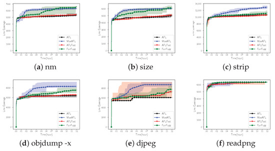
Figure 6.
Line coverage per time. Each solid line is average line coverage of each fuzzer. The background colors describe the range between the maximum and minimum line coverage.
Table 2.
Line coverage after 12 h fuzzing. We described the line coverage of each fuzzer in absolute number of lines and percentage of a total lines. We also provide variance of final line coverage in 8 independent experiments.
Out of six test binaries, MaxAFL outperformed the original AFL in five binaries. MaxAFL showed improved performance compared with AFLFast in all test binaries. FairFuzz gained more line coverage compared with MaxAFL in just 2 binaries. If we look at the detailed result, in the case of nm, although the line coverage of FairFuzz was 6597 which is the best performance among the fuzzers, the line coverage of MaxAFL was not significantly different which is 6348. However, AFL and AFLFast showed 5351 and 5380 line coverage, respectively. In the case of size, it was found that FairFuzz covered just 76 lines more compared with MaxAFL. If we compare the result of MaxAFL with results of AFL and AFLFast, MaxAFL gained 1000 more line coverage. The result of strip, as shown in Figure 6c, showed that the line coverage steadily increased throughout the entire fuzzing process, and finally, MaxAFL showed the best performance among four fuzzers. In the case of objdump, which is the largest target among our test targets, the performance is also improved. Performance improvement in objdump was about 30.13% compared with the original AFL, which is the biggest improvement in binutils binaries. MaxAFL covered 781 lines more compared with FairFuzz. Djpeg of libjpeg, which receives a JPEG image as an input file, showed the greatest performance improvement among the test targets. A total of 3719 lines more were tested compared with the original AFL. Finally, in the case of readpng that receives a PNG file as an input, it was found that there is little difference in performance among the tested fuzzers. The performance results were in the order of AFL, MaxAFL, AFLFast, and FairFuzz. However, the difference of line coverage between AFL and MaxAFL was just two; this is statistically negligible.
In conclusion, we compared MaxAFL with three other AFL-based fuzzers on six Linux binaries for 12 h and found that MaxAFL showed the best line coverage metric, on average, on three binaries. In the other three binaries, MaxAFL showed second performance among four fuzzers and there was no remarkable performance difference with the fuzzer which showed the best line coverage.

- RQ2. Is the mutation of MaxAFL more efficient than the other fuzzers?
Secondly, to check the effectiveness of MaxAFL’s mutation using gradient descent, we limited the maximum number of executions of fuzzers and compared the performance of MaxAFL with the other fuzzers: AFL, AFLFast, and FairFuzz. Note that, approximately, one test target execution means one mutation of the input. Therefore, we can say that the mutation action of the fuzzer, which shows better performance in this experiment, is more efficient than the others without considering execution speed. Each experiment was conducted by comparing the line coverage obtained by each fuzzer during 12 million executions. However, in the case of djpeg, the execution speed was extremely slow, so the maximum number of execution was limited to 0.7 million rather than 12 million. In this experiment, a total of eight independent experiments were performed and we aggregated and analyzed all eight results. The results of line coverage per executions are shown in Figure 7, and the detailed final results are shown in Table 3.
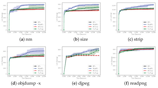
Figure 7.
Each solid line is average line coverage of each fuzzer. The background colors describe the range between the maximum and minimum line coverage.
Table 3.
Line coverage after 12M executions. We described the line coverage of each fuzzer in absolute number of lines and percentage of a total lines. We also provide variance of final line coverage in eight independent experiments.
As a result of the experiment of RQ2, MaxAFL showed better performance than that of RQ1. Out of 6 binaries, MaxAFL showed the best line coverage per program execution on five binares. In the case of nm, a total line coverage increased by 1143 lines on MaxAFL, showing a performance improvement of 22.50% compared with AFL. The difference of line coverage between FairFuzz and MaxAFL is 823 which is meaningful improvement. Compared with the results of RQ1, it showed that there is more performance improvement. In the case of size, MaxAFL tested 613 more lines compared with FairFuzz. In RQ1, FairFuzz outperformed MaxAFL slightly, however, MaxAFL outperformed FairFuzz in RQ2. Next, in the case of strip, MaxAFL showed 21.19% better performance than AFL and it is the greatest result among the tested fuzzers. In the case of objdump, the biggest binary in our tested target, MaxAFL also showed improved performance. AFL, AFLFast and FairFuzz showed less than 7000 line coverage, however, MaxAFL showed 8128 line coverage that is outstanding improvement. Djpeg showed a total increase of 2674 line coverage compared with AFL, which means that the performance of MaxAFL is improved by about 44.15%. Finally, readpng suffered a −0.66% performance drop compared with AFL, worse than the result of RQ1. However, it was just a decrease of 41 line coverage.
In conclusion, as a result of comparing the performance of MaxAFL and the other three fuzzers by limiting the maximum number of binary executions, MaxAFL showed the best results on five binaries. This means that MaxAFL’s mutation process is more efficient than mutation actions of the other fuzzers. The results of RQ2 are much better than the results of RQ1, which means that our fuzzer has a performance advantage in terms of mutation action more than execution speed.

- RQ3. Can MaxAFL find more bugs than the other fuzzers?
To evaluate the important goal of the fuzzer, bug finding ability, we ran our fuzzer with LAVA-M [41] dataset and compared the results with the other fuzzers. We checked how many unique bugs were found by fuzzing for 12 h on four bug-injected binaries (who, uniq, md5sum, and base64). A total of eight repeated experiments were conducted and the best results were compared. The experimental results are shown in Table 4.
Table 4.
Number of unique crashes found by each fuzzer.
As a result of the experiment, in the case of base64, we found 47 more crashes compared with AFL. We found three crashes unlisted by LAVA author because we could trigger injected bugs that LAVA authors could not trigger. In the case of other binaries, there were no significant differences from the other fuzzers. Table 5 shows a list of all bugs found by MaxAFL.
Table 5.
List of found bugs by MaxAFL. Each number is unique number that LAVA author defined.

8. Discussion
As a result of our experiment, MaxAFL showed better results than the other AFL-based fuzzers, generally. However, in some cases such as readpng in RQ1 and RQ2, there was no significant improvement in code coverage compared with the existing fuzzers. Moreover, in the RQ3 experiment results, MaxAFL could find more bugs than the other fuzzers in base64, but MaxAFL could not find more bugs in the other binaries. In some cases, even though the performance improvement obviously occurred, the percentage of the tested source code was low. For example, in the case of nm, the line coverage was improved by 18.63% compared with the original AFL, but only 6.4% of the entire source code was tested.
Of course, designing a fuzzer that shows great performance in all cases is almost impossible. However, the results that are mentioned above are limitations of our approach. We can guess the reasons for these limitations as follows.
First, the optimization problem which we defined is not perfect and may not work effectively in some cases. Our objective function is constructed using the heuristic method and it is not smooth and continuous. Furthermore, the dimension of the variable is the same as the length of the input, and each element of the variable is also limited to an integer from 0 to 255. Our approach used the approximation of the subgradient instead of the accurate gradient. For these reasons, in some binaries, the constraints cannot be solved effectively by the gradient-based optimization algorithm, and the performance improvement may not occur.
Second, since the seed inputs are not varied and there may be a code region that cannot be tested by changing the input, the percentage of the line coverage can be measured low. Mutation-based fuzzers based on AFL basically generate new input values by modifying the small bytes of the existing input, so they cannot create completely new types of input. Therefore, the code coverage may be measured differently depending on how the initial seed inputs are configured. In addition, if optional arguments (e.g., -x of objdump command) or environment variables (e.g., $HOME$ in Linux) are used in the tested binary, there are the code areas that cannot be executed by modifying input values. These areas of source code cannot be tested with our fuzzing method, so absolute line coverage can be measured low.
To solve these limitations, we will design the optimization problem more precisely in the future. Based on numerous experiments, we plan to refine the objective function and the optimization technique that works effectively in most cases through statistical analysis. We will increase the number of the test binaries and the seed inputs for evaluation, and use a different dataset for testing bug-finding ability other than LAVA-M.
9. Conclusions
In this paper, we have presented MaxAFL, a novel gradient-based fuzzer based on AFL. We used a lightweight static analysis to calculate MEIC and generated the objective function using MEIC and branch variables. After that, we applied the gradient descent algorithm to generate efficient inputs by minimizing the objective function. We proposed the simple techniques such as probabilistic mutation during the optimization process and adaptive objective function which helps to search for various paths. We alternated the deterministic stage of AFL to improve the efficiency of AFL’s mutation actions. The results show that MaxAFL outperformed the existing fuzzers in all metrics that we tested: line coverage per time, line coverage per total execution, number of unique crashes. In future, we plan to design a more accurate objective function to increase performance. We will also apply the state of the art gradient-based optimization algorithm to MaxAFL.
Author Contributions
All authors contributed to this work. Conceptualization, Y.K.; methodology, Y.K. and J.Y.; software, Y.K.; validation Y.K. and J.Y.; writing—original draft preparation, Y.K.; writing—review and editing, J.Y.; visualization, Y.K. and J.Y.; supervision, J.Y.; project administration, J.Y. All authors have read and agreed to the published version of the manuscript.
Funding
This research received no external funding.
Institutional Review Board Statement
Not applicable.
Informed Consent Statement
Not applicable.
Data Availability Statement
Data sharing not applicable. No new data were created or analyzed in this study. Data sharing is not applicable to this article.
Acknowledgments
Ji Won Yoon was supported by the Institute for Information and Communications Technology Promotion (IITP) grant funded by the Korea government (MSIT) (no. 2017-0-00545).
Conflicts of Interest
The authors declare no conflict of interest.
Abbreviations
The following abbreviations are used in this manuscript:
| MEIC | Maximum Expectation of Instruction Count |
References
- Miller, B.P.; Fredriksen, L.; So, B. An empirical study of the reliability of UNIX utilities. Commun. ACM 1990, 33, 32–44. [Google Scholar] [CrossRef]
- Zalewski, M. American Fuzzy Lop. 2017. Available online: http://lcamtuf.coredump.cx/afl (accessed on 23 December 2020).
- Böhme, M.; Pham, V.T.; Roychoudhury, A. Coverage-based greybox fuzzing as markov chain. IEEE Trans. Softw. Eng. 2017, 45, 489–506. [Google Scholar] [CrossRef]
- Lemieux, C.; Sen, K. Fairfuzz: A targeted mutation strategy for increasing greybox fuzz testing coverage. In Proceedings of the 33rd ACM/IEEE International Conference on Automated Software Engineering, Montpellier, France, 3–7 September 2018; pp. 475–485. [Google Scholar]
- Stephens, N.; Grosen, J.; Salls, C.; Dutcher, A.; Wang, R.; Corbetta, J.; Shoshitaishvili, Y.; Kruegel, C.; Vigna, G. Driller: Augmenting Fuzzing Through Selective Symbolic Execution. In Proceedings of the NDSS, San Diego, CA, USA, 21–24 February 2016; Volume 16, pp. 1–16. [Google Scholar]
- Yun, I.; Lee, S.; Xu, M.; Jang, Y.; Kim, T. {QSYM}: A practical concolic execution engine tailored for hybrid fuzzing. In Proceedings of the 27th {USENIX} Security Symposium ({USENIX} Security 18), Baltimore, MD, USA, 15–17 August 2018; pp. 745–761. [Google Scholar]
- Chen, P.; Chen, H. Angora: Efficient fuzzing by principled search. In Proceedings of the 2018 IEEE Symposium on Security and Privacy (SP), San Francisco, CA, USA, 20–24 May 2018; pp. 711–725. [Google Scholar]
- She, D.; Pei, K.; Epstein, D.; Yang, J.; Ray, B.; Jana, S. NEUZZ: Efficient fuzzing with neural program smoothing. In Proceedings of the 2019 IEEE Symposium on Security and Privacy (SP), San Francisco, CA, USA, 19–23 May 2019; pp. 803–817. [Google Scholar]
- Myers, G.J.; Badgett, T.; Thomas, T.M.; Sandler, C. The Art of Software Testing; John Wiley & Sons: Hoboken, NJ, NSA, 2004; Volume 2. [Google Scholar]
- Klees, G.; Ruef, A.; Cooper, B.; Wei, S.; Hicks, M. Evaluating fuzz testing. In Proceedings of the 2018 ACM SIGSAC Conference on Computer and Communications Security, Toronto, ON, Canada, 15–19 October 2018; pp. 2123–2138. [Google Scholar]
- Goodfellow, I.; Bengio, Y.; Courville, A. Deep Learning; MIT Press: Cambridge, MA, USA, 2016; Available online: http://www.deeplearningbook.org (accessed on 23 December 2020).
- Van Laarhoven, P.J.; Aarts, E.H. Simulated annealing. In Simulated Annealing: Theory and Applications; Springer: Berlin/Heidelberg, Germany, 1987; pp. 7–15. [Google Scholar]
- Kirkpatrick, S.; Gelatt, C.D.; Vecchi, M.P. Optimization by simulated annealing. Science 1983, 220, 671–680. [Google Scholar] [CrossRef] [PubMed]
- Hu, X.; Shonkwiler, R.; Spruill, M.C. Random Restarts in Global Optimization. 2009. Available online: https://smartech.gatech.edu/bitstream/handle/1853/31310/1192-015.pdf?sequence=1&isAllowed=y (accessed on 23 December 2020).
- Serebryany, K. libFuzzer—A Library for Coverage-Guided Fuzz Testing. 2015. Available online: https://llvm.org/docs/LibFuzzer.html (accessed on 23 December 2020).
- The LLVM Compiler Infrastructure Project. 2020. Available online: https://llvm.org/ (accessed on 23 December 2020).
- Swiecki, R. Honggfuzz: A General-Purpose, Easy-to-Use Fuzzer with Interesting Analysis Options. Available online: https://github.com/google/honggfuzz (accessed on 23 December 2020).
- Böhme, M.; Pham, V.T.; Nguyen, M.D.; Roychoudhury, A. Directed greybox fuzzing. In Proceedings of the 2017 ACM SIGSAC Conference on Computer and Communications Security, Dallas, TX, USA, 30 October–3 November 2017; pp. 2329–2344. [Google Scholar]
- Pham, V.T.; Böhme, M.; Santosa, A.E.; Caciulescu, A.R.; Roychoudhury, A. Smart greybox fuzzing. IEEE Trans. Softw. Eng. 2019. [Google Scholar] [CrossRef]
- Gan, S.; Zhang, C.; Qin, X.; Tu, X.; Li, K.; Pei, Z.; Chen, Z. Collafl: Path sensitive fuzzing. In Proceedings of the 2018 IEEE Symposium on Security and Privacy (SP), San Francisco, CA, USA, 20–24 May 2018; pp. 679–696. [Google Scholar]
- De Moura, L.; Bjørner, N. Z3: An efficient SMT solver. In International Conference on Tools and Algorithms for the Construction and Analysis of Systems; Springer: Berlin/Heidelberg, Germany, 2008; pp. 337–340. [Google Scholar]
- Cadar, C.; Dunbar, D.; Engler, D.R. Klee: Unassisted and automatic generation of high-coverage tests for complex systems programs. In Proceedings of the OSDI’08: 8th USENIX Conference on Operating Systems Design and Implementation, San Diego, CA, USA, 10–11 December 2008; Volume 8, pp. 209–224. [Google Scholar]
- Godefroid, P.; Levin, M.Y.; Molnar, D.A. Automated Whitebox Fuzz Testing. In Proceedings of the NDSS, San Diego, CA, USA, 10–13 February 2008; Volume 8, pp. 151–166. [Google Scholar]
- Bounimova, E.; Godefroid, P.; Molnar, D. Billions and billions of constraints: Whitebox fuzz testing in production. In Proceedings of the IEEE 2013 35th International Conference on Software Engineering (ICSE), San Francisco, CA, USA, 18–26 May 2013; pp. 122–131. [Google Scholar]
- Godefroid, P.; Klarlund, N.; Sen, K. DART: Directed automated random testing. In Proceedings of the 2005 ACM SIGPLAN conference on Programming Language Design and Implementation, Chicago, IL, USA, 12–15 June 2005; pp. 213–223. [Google Scholar]
- Haller, I.; Slowinska, A.; Neugschwandtner, M.; Bos, H. Dowsing for Overflows: A Guided Fuzzer to Find Buffer Boundary Violations. In Proceedings of the 22nd USENIX Security Symposium (USENIX Security 13), Washington, DC, USA, 14–16 August 2013; pp. 49–64. [Google Scholar]
- Zhao, L.; Duan, Y.; Yin, H.; Xuan, J. Send Hardest Problems My Way: Probabilistic Path Prioritization for Hybrid Fuzzing. In Proceedings of the NDSS, San Diego, CA, USA, 24–27 February 2019. [Google Scholar]
- Choi, J.; Jang, J.; Han, C.; Cha, S.K. Grey-box concolic testing on binary code. In Proceedings of the 2019 IEEE/ACM 41st International Conference on Software Engineering (ICSE), Montreal, QC, Canada, 25–31 May 2019; pp. 736–747. [Google Scholar]
- Chen, P.; Liu, J.; Chen, H. Matryoshka: Fuzzing deeply nested branches. In Proceedings of the 2019 ACM SIGSAC Conference on Computer and Communications Security, London, UK, 11–15 November 2019; pp. 499–513. [Google Scholar]
- Böttinger, K.; Godefroid, P.; Singh, R. Deep reinforcement fuzzing. In Proceedings of the 2018 IEEE Security and Privacy Workshops (SPW), San Francisco, CA, USA, 24 May 2018; pp. 116–122. [Google Scholar]
- Drozd, W.; Wagner, M.D. Fuzzergym: A competitive framework for fuzzing and learning. arXiv 2018, arXiv:1807.07490. [Google Scholar]
- Rajpal, M.; Blum, W.; Singh, R. Not all bytes are equal: Neural byte sieve for fuzzing. arXiv 2017, arXiv:1711.04596. [Google Scholar]
- Godefroid, P.; Peleg, H.; Singh, R. Learn&fuzz: Machine learning for input fuzzing. In Proceedings of the 2017 32nd IEEE/ACM International Conference on Automated Software Engineering (ASE), Urbana, IL, USA, 30 October–3 November 2017; pp. 50–59. [Google Scholar]
- Writing an LLVM Pass. 2020. Available online: https://llvm.org/docs/WritingAnLLVMPass.html (accessed on 23 December 2020).
- Google/AFL. Available online: https://github.com/google/AFL (accessed on 15 August 2020).
- GNU Binutils. Available online: https://www.gnu.org/software/binutils/ (accessed on 14 August 2020).
- libjpeg. Available online: https://www.ijg.org/ (accessed on 14 August 2020).
- libpng. Available online: http://www.libpng.org/pub/png/libpng.html (accessed on 14 August 2020).
- MozillaSecurity/Fuzzdata. Available online: https://github.com/MozillaSecurity/fuzzdata (accessed on 15 August 2020).
- Google/Fuzzer-Test-Suite. Available online: https://github.com/google/fuzzer-test-suite (accessed on 15 August 2020).
- Dolan-Gavitt, B.; Hulin, P.; Kirda, E.; Leek, T.; Mambretti, A.; Robertson, W.; Ulrich, F.; Whelan, R. Lava: Large-scale automated vulnerability addition. In Proceedings of the 2016 IEEE Symposium on Security and Privacy (SP), San Jose, CA, USA, 22–26 May 2016; pp. 110–121. [Google Scholar]
- GNU Coreutils. Available online: https://www.gnu.org/software/coreutils/ (accessed on 18 August 2020).
Publisher’s Note: MDPI stays neutral with regard to jurisdictional claims in published maps and institutional affiliations. |
© 2020 by the authors. Licensee MDPI, Basel, Switzerland. This article is an open access article distributed under the terms and conditions of the Creative Commons Attribution (CC BY) license (http://creativecommons.org/licenses/by/4.0/).