Article

Predicting the Material Footprint in Germany between 2015 and 2020 via Seasonally Decomposed Autoregressive and Exponential Smoothing Algorithms

1
Wuppertal Institute for Climate, Environment and Energy, Doeppersberg 19, 41203 Wuppertal, Germany
2
Industrial Design, Folkwang University of the Arts, Klemensborn 39, 45239 Essen, Germany
*
Author to whom correspondence should be addressed.
Resources 2020, 9(11), 125; https://doi.org/10.3390/resources9110125
Submission received: 14 June 2020 / Revised: 18 September 2020 / Accepted: 5 October 2020 / Published: 25 October 2020

Abstract

:
Recent research on the natural resource use of private consumption suggests a sustainable Material Footprint of 8 tons per capita by 2050 in industrialised countries. We analyse the Material Footprint in Germany from 2015 to 2020 in order to test whether the Material Footprint decreases accordingly. We studied the Material Footprint of 113,559 users of an online footprint calculator and predicted the Material Footprint by seasonally decomposed autoregressive (STL-ARIMA) and exponential smoothing (STL-ETS) algorithms. We find a relatively stable Material Footprint for private consumption. The overall Material Footprint decreased by 0.4% per year between 2015 and 2020 on average. The predictions do not suggest that the Material Footprint of private consumption follows the reduction path of 3.3% per year that will lead to the sustainable consumption of natural resources.

1. Introduction

In the majority of industrialised countries, the total material requirements associated with consumption activities, including unused material extraction or hidden flows (i.e., the Total Material Consumption—TMC), per capita per year are an average of 40 to 50 tons [1]. The demand for natural resources affects the world’s ecosystem and places a burden on efforts to counter environmental pollution and climate change. According to the International Resource Panel [2], global resource extraction has accelerated over the past two decades and is responsible for nearly 50% of global greenhouse emissions (GHG) and for over 90% of global biodiversity loss and water stress. In contrast, Lettenmeier et al. [3,4] advocated a sustainable Material Footprint (i.e., the Total Material Consumption by private households) of 8 tons per capita per year by 2050. Bringezu [5,6] suggests a target corridor of 6–12 tons of TMC per capita for 2050. As a consequence, policies on the consumption of natural resources should target a reduction in the consumption of natural resources by at least 80% or a factor of five from the present average.
For instance, Germany shows an ambitious record of policies on sustainable consumption and sustainable resource management. In 2002, Germany published its first sustainability strategy. In 2016, the German sustainability strategy adopted the framework of the Sustainable Development Goals (SDGs) [7] introduced by the United Nations in 2015 [8]. Sustainable Development Goal 12 encourages more sustainable consumption and production by minimising the use of natural resources. Germany set up a national strategy specifically on natural resource management and resource efficiency in 2012—the German Resource Efficiency Programme (ProgRess). On a European level, Germany´s specified strategy is regarded as “pioneering” [9]. Since then, Germany´s government have updated ProgRess with regard to goals, guidelines and approaches. In this respect, the ProgRess addresses the goals stated in the German sustainability strategy and strives to implement the SDGs on resource efficiency [10].
Concerning resource efficiency, Germany aims to double raw material productivity by 2020 relative to 1994. However, the latest available environmental accounting data show an increase in resource productivity of only 48.8% in 2014 relative to 1994. Since 2010, there has been no increasing trend suggesting that the country will achieve doubled productivity by 2020 [11].
More recently, in 2019, Germany updated its National Program for Sustainable Consumption and specifically identified relevant consumer policies. The program concludes that behavioural changes are necessary in favour of more resource-efficient consumption. However, behavioural change faces obstacles such as a lack of information, personalised feedback and fear of justification in one’s social surroundings. The program suggests providing personalised information and feedback via carbon and resource calculators [12]. In 2007, the German Environmental Agency (UBA) developed a carbon footprint calculator. However, a Material Footprint calculator was only published online by the Wuppertal Institute for Environment, Climate and Energy in 2015 (the Material Footprint calculator, including all questions and items, can be accessed in full at ressourcen-rechner.de/?lang=en). The Material Footprint calculator by the Wuppertal Institute enables consumers to analyse their resource use and gives personalised feedback on how to reduce their personal Material Footprint based on individual results.
Internationally, Germany can be considered a pioneer thanks to their implementation of a national strategy on resource efficiency in 2012, which, throughout its updates, addresses the reduction in reduce consumption by private households. Germany´s early implementation of a national strategy specifying resource efficiency allows us to evaluate whether its strategy effectively reduces the resource use of private households towards a sustainable level. In this respect, we are able to present findings from a Material Footprint calculator surveying the resource consumption of private households since 2015 based on the information of its 113,559 users. Against this background, the goal of this paper is to show the trend of the Material Footprint by private households from 2015 to 2020. In this way, we aim to show whether the trend of the Material Footprint has reduced in the past five years, ultimately meeting the goal of a Material Footprint of about eight tons by 2050. Therefore, we develop a prediction model which allows us to forecast the Material Footprint accurately in the near future.
We start by introducing the data of the footprint calculator and the underlying Material Footprint calculations in Section 2. Here, we introduce the development of the Material Footprint as an indicator for resource use. In Section 3, we describe the methods applied to predict the Material Footprint until 2020. Section 4 presents descriptive results of the Material Footprint in the past five years in relation to the overall Material Footprint, as well as in regard to nutrition, housing, mobility, for consumer goods, leisure activities and vacations. Section 4 also presents the results of predicting the overall Material Footprint in relation to nutrition, housing and mobility until 2020. Section 5 discusses the sampling and methods, summarises the findings and draws conclusions on the effectiveness on consumer policies addressing sustainable resource management.

2. Materials

2.1. Data

Material Footprint calculations are based on lifecycle material inputs of all goods and services in private households. The Material Footprint was first introduced by Lettenmeier et al. [13] as the “ecological rucksack”. In the original sense, and also used in this study, the Material Footprint of a service is the cradle-to-cradle material input needed to generate a product or service, including unused extraction or hidden material flows (i.e., the eventual Total Material Consumption of private households). The Material Footprint is calculated using life cycle analysis (LCA) linked to the life cycle inventory (LCI) database ecoinvent from 2015 (see also [14,15,16], and, for a more extensive description of the method [17,18,19,20,21,22]).
The material inputs encompass the natural resources required for raw material extraction, and the production and use of processed materials, products and services for private consumption. Natural resources include abiotic and biotic raw materials from used extraction (put to economic use) and unused extraction (e.g., overburden from mining). By taking unused extraction into account, the Material Footprint covers the Total Material Consumption of private households for products or services.
More recently, the term Material Footprint has been used in national environmental accounting as a consumption-based indicator (including imports) that accounts for the domestic extraction of all raw materials in terms of raw material equivalents (RME), but not the unused extracted material [23]. For example, Giljum et al. [24] exclude exports and refer to Raw Material Consumption (RMC) as the Material Footprint (MF) by applying a global, multiregional input–output (IO) model (MRIOT). Lutter et al. [25] give an overview of approaches to calculate Material Footprints based on IO data.
Other recent studies use aggregated IO tables to derive material intensities (e.g., in terms of kg/EUR) and national survey expenditure data in order to give a more differentiated picture of the Material Footprint of private consumption [26,27,28,29,30,31,32,33,34,35]. Such approaches imply a direct relation between the expenditure and resource use of private households. However, higher expenditure may not necessarily result in higher Material Footprints. Consumers may as well shift consumption to more expensive high-quality goods with lower material intensity.
Our data differ from the approaches by relying on consumer data collected in a single survey. The calculation of the Material Footprint in this study is based on the total lifecycle material flow accounting of the consumption of products and services directly stated by consumers in the survey. In this way, we do not rely on assumptions on the resource intensities (or carbon intensities) of expenditure. Buhl [26] highlights that relying on resource intensities based on IO data does not allow us to attribute specific intensities to commodities, only allowing us to attribute a common, average resource intensity for mobility expenditure rather than differentiating mobility by air travel, car travel or mobility by bike (also discussed in [28,29]). Buhl et al. [30] addressed this issue by introducing LCA data in order to identify disaggregated resource intensities in mobility. However, they acknowledge that combing expenditure data and resource intensities still assumes a strict proportional relation between expenditure and resource consumption that may bias results.
In contrast, calculations based on life cycle assessments of survey data rather than on national material flow accounting in input–output modelling enable researchers to draw a more direct, more differentiating picture of the Material Footprint of private households in different consumption categories. This approach does not suffer from aggregated resource use of national flow accounting (IO data) and does not rely on assumptions of the resource intensity of expenditure data.
We differentiate between six categories of private consumption: (1) nutrition, (2) housing, (3) mobility, (4) consumer goods, (5) leisure and (6) vacations.
(1)
Nutrition includes diets, food waste and all foodstuffs and drinks consumed;
(2)
Mobility includes everyday transport such as commuting and leisure activities by car, motorcycle, bicycle and public mobility;
(3)
Construction and housing include the use of energy (electricity and heating) for household purposes;
(4)
Consumer goods include clothes, furniture, household appliances such as refrigerators and washing machines, and consumer electronics such as TV sets and tablets;
(5)
Leisure activities include hobbies such as sports and cultural activities;
(6)
Vacations include travel and accommodation.
In contrast to studies on resource use by private households relying on expenditure data covering consumption categories according to the Classification of Individual Consumption by Purpose (COICOP), the survey does not comprise education and health. Buhl et al. [15] compare the findings of the Material Footprint calculations based on expenditure data and based on data from the footprint calculator, as presented. They find that education accounts for around 0.3 tons per capita and health for around 1.4 tons per capita. Both account for around 5% of the overall Material Footprint of private consumption, resulting in a slightly lower overall Material Footprint. They already highlight that the most relevant categories are housing, mobility and nutrition.
The Material Footprint calculator also surveys personal and household data of users. The influence of personal and household features like income on the Material Footprint has already been covered elsewhere and is thus not the subject of the following analysis (see [14,15,16]).
After preparing the data and removing invalid and implausible responses, information provided by 113,559 users between its launch on 25 February 2015 and 19 December 2019 was analysed. The data consist of pooled information of different users across the years. About 10% of the data were surveyed in 2015, 15% in 2016, 30% in 2017, 27% in 2018 and 18% in 2019. The footprint calculator was most popular in 2017 and 2018 and least popular at the start of 2015. Hence, we expect the highest uncertainty of predictions at the beginning of 2015. About 60% of the users provided additional socioeconomic information. The varying number of observations between single variables is due to implausible responses and missing data due to non-response. We excluded the highest one per cent of observations of the distribution in order to address outliers and implausible responses.
Table 1 provides an overview of the Material Footprints as well as the users´ ages and the share of female users.
The application can be used for free; there are no incentives involved, and participation is voluntary. Accordingly, the quality of the data suffers from self-selection and shows a high share of females and a low average age of users. According to the latest national census in Germany in 2011, the average age in Germany was 44 years, while 51% of the population was female [36].

2.2. Weighting

Given the non-representative sample for Germany, we make use of a weighting algorithm developed for the American National Election Study (AWA). AWA uses an iterative, multiplicative raking model to identify weights [37]. In the AWA, survey marginals for a given set of variables are compared to known population marginals for each variable of interest. In a series of steps, the survey proportions for each variable are compared to known population proportions for the same variables and adjusted to match those figures.
Like all weighting procedures, raking is also sensitive to the number and nature of the variables used for correction. As more variables are introduced, the variance of weights will tend to increase. Similarly, as raking variables become more discrepant from known population parameters, corrections to eliminate biases will tend to increase variance, thus affecting the consistency of estimations in further statistical analyses. In this sense, variable selection for raking is a balancing act between eliminating bias and minimising variance in the data.
We selected sex and age for raking. Table 1 shows a considerably younger sample and a higher share of female respondents than the average in Germany. Importantly, the German census provides reliable and distinct data of the overall population in Germany for sex and age. In this way, we keep the design effect of weighting as small as possible and the prediction accuracy as high as possible.
Table 2 shows the shares of sex and age groups in the sample and the actual shares according to the latest national census data in Germany. For instance, females account for 63% in the sample, but actually only 51% are female in the population. In AWA, each female gets weighted by w 1 = 51 / 63 . We also find that 10% of our sample consists of of age < 18, while 16% are actually age < 18 in the German population. Hence, w 1 is multiplied by w 2 = 16 / 10 . This multiplicative procedure continuous for all w k = 1 k w until the sample margins and population margins do not converge any further.
Table 2 shows the results of the raking.
After raking the data, the weighted data fit the shares of sex in the census perfectly. The shares of age groups in the weighted data fit the census data not perfectly, but closely, except the age group > 75. Eventually, the weighted data give a more representative picture of the Material Footprints.

3. Methods

We use season–trend decomposition using loess (STL) with autoregressive (ARIMA) and exponential smoothing (ETS) algorithms to predict and forecast the overall Material Footprint as well as in relation to housing, mobility and nutrition in Germany between 2015 and 2020. STL-ARIMA and STL-ETS have been successfully applied to predict and forecast energy demand [38,39] or CO2 emissions [40]. We first describe the autoregressive models and exponential smoothing. We then describe the season–trend decomposition applied to our data. In Section 4, we report the prediction accuracy of the proposed models.

3.1. ARIMA

In autoregressive modelling, we predict the Material Footprint ( y ) at time t using a linear combination of past values of the variable at time t p .
The term autoregression (AR) indicates that it is a regression of the variable against itself. Moving Average Models (MA) do not use past values of the forecast variable in a regression, but instead use unobserved past forecast errors ( ε ) at time t q in a regression-like model. If we combine AR and MA processes, we arrive at Autoregressive Integrated MA models (ARIMA). By differencing, ARIMA processes become stationary with constant means and equal variance.
An ARIMA process can be written as
y d t = c + ϕ 1 y d t 1 + + ϕ p y d t p + θ 1 ε t 1 + + θ q ε t q + ε t
where c is the intercept, and ϕ and θ are the predicted coefficients of y and ε , respectively.
For convenience, we introduce a backshift operator B for describing the differencing process.
y d t = ( 1 B ) d y t  
Then, a non-seasonal ARIMA process is given by
( 1 B ) d y t = c + φ ( B ) y t + θ ( B ) ε t  
However, we hypothesise that there is a seasonal part to our time series. Therefore, we model an ARIMA process by multiplying the non-seasonal parts with the seasonal parts of the time series.
( 1 B m ) D ( 1 B ) d y t = c +   Φ ( B m ) φ ( B ) y t +   Θ ( B m ) θ ( B ) ε t
where m = number of observations per year (i.e., 12 given monthly data), and d is the number of required differences for the seasonal and D non-seasonal parts, respectively. φ ( z ) and θ ( z ) are polynomials of order p and q for the non-seasonal parts and Φ ( z ) and Θ ( z ) are polynomials of orders P and Q for the seasonal parts.
In order to find an optimal model order, that is, values for p , q , d ,   P , Q , D , we follow the proposed algorithm by Hyndman and Khandakar [41]. First, we test for seasonality (according to [42]) in order to test whether we need to introduce a seasonal part to our model. After D is selected, we test for stationarity and choose d (according to [43]). After we determine the number of differences, we find the lag values ( p , q , P , Q ) by minimising the Akaike Information Criterion (AIC):
A I C = 2   l o g ( L )   +   2 ( p + q + P + Q + k )
where k =   1 if c     0 and 0 otherwise, and L is the maximised likelihood of the model fitted, as described in (4). However, it is not feasible to fit every potential model and find the one with the lowest AIC. Therefore, Hyndman and Khandakar [41] propose a stepwise selection algorithm for finding the model order efficiently. In the first step, we consider 4 initial models to start with and find the one with the lowest AIC. In a second step, up to 13 variations on the initially selected models are considered in the search for the model with the lowest AIC. The second step is repeated until no lower AIC can be found.

3.2. ETS

Alternatively, we consider exponential smoothing (ETS). In ETS, predictions (or fits) and forecasts are computed by weighted averages, where the weights decrease exponentially as observations come from further in the past ([44]):
y ^ t + 1 | t = α y t + ( 1 α ) y ^ t + 1 | t 1
Predictions at time t + 1 are weighted averages between the most recent observation y t and the previous predictions y ^ t + 1 | t 1 or forecasts y ^ T + | 1 T 1 and 0 < α < 1 is the smoothing parameter. In component form, we substitute the smoothened values at t time or h , forecast as the level of smoothing l t = y ^ t + 1 | t = y ^ t + 1 | h .
We use simple exponential smoothing with multiplicative errors if seasonal variation is not constant over time. ETS models with multiplicative errors can be noted by one-step-ahead errors as relative errors: ε t = y t y ^ t | t 1 y ^ t | t 1 .
The multiplicative form of the ETS model is then
y t = l t 1 ( 1 + ε t )
or an ETS ( M , N , N ) in state space notation, where M denotes a multiplicative error; ( N , N ) denotes the trend and seasonal component in simple exponential smoothing [43].

3.3. STL

In order to properly identify trends and seasonality in our data, we decompose the data into seasonal and trend components using locally weighted regression (loess) smoothing (STL) ([45]). Here, data Y are decomposed additively into trend ( T ), season ( S ) and remainder ( R ) components at a given time t .
Y t S t   = T t + R t
STL can identify any type of seasonality and the seasonal component is allowed to change over time (in contrast to univariate seasonal ARIMA). ARIMA and ETS, respectively, are then applied to the seasonally adjusted, i.e., non-seasonal part of the data.
In order to identify the seasonal component, a loess regression is conducted. The seasonal smoothing is then identified in the q th span by assigning a neighbourhood weight v for each observation x i
v i ( x )   = ω ( x i x δ q ( x ) )
where ω is a tricubic weight function and d is the distance of the farthest x i to x in q of x i to x in q . Thus, x i closer to x have the larger weights.
The seasonal part of the last year is added to the ARIMA and ETS forecast, ignoring the uncertainty of the seasonal part underlying the forecast. This is justified, since seasonal components do change slowly relative to the seasonally adjusted parts.
In order to test the accuracy of the forecast model, we report commonly reported forecast errors: root mean squared error (RMSE), mean absolute error (MAE), mean absolute percentage error (MAPE) and the mean absolute scaled error (MASE). The scaled error is the forecast error MAE relative to the MAE for a naïve seasonal forecast on the training data Q .
MASE   = MAE Q
The mean absolute error (MAE) is given by
MAE = m e a n ( | ε t | ) = m e a n ( | y t y ^ t | N | )
for t = N + 1 , T , where ( y 1 , , y T ) are the test data and ( y 1 , , y N ) are the training data. To check the accuracy of our forecasting method, we estimate the parameters using the training data, and forecast the next T N observations. We select the last observed year as test data and forecast the earlier observed years on the last year´s data. These forecasts can then be compared to the test data observed.
The scaling statistic Q of the naïve forecast on the training data is defined as the mean absolute difference between consecutive observations of m seasons and j forecasts ([46]):
Q   = 1 N m j = m + 1 N | y j y ^ j m |
Then, we can check whether STL-ARIMA or STL-ETS is more accurate than a naïve seasonal forecast. MASE is straightforward to interpret. With MASE = 1, the MAE of the seasonal naïve forecast is equal to MAE of the STL-ARIMA or STL-ETS. With MASE < 1, the STL-ARIMA is more accurate with a lower forecast error than a naïve forecast.

4. Results

4.1. Time Series Analyses

In the following, we present a time series analysis of the Material Footprint by private households in Germany between 2015 and 2019. Figure 1 shows the Material Footprint by consumption category. It is notable that no relevant change or decrease in the Material Footprint can be observed. The categories of mobility, housing and nutrition cover more than 80% of the overall Material Footprint. Moreover, Buhl et al. [15] predict the overall Material Footprint by a linear combination of nutrition, housing and mobility and are able to explain 91% of the variation in the overall Material Footprint. Respondents who report higher resource use in nutrition, mobility and housing are likely to report higher Material Footprints in leisure, vacation or consumer goods as well, and thus a higher Material Footprint overall.
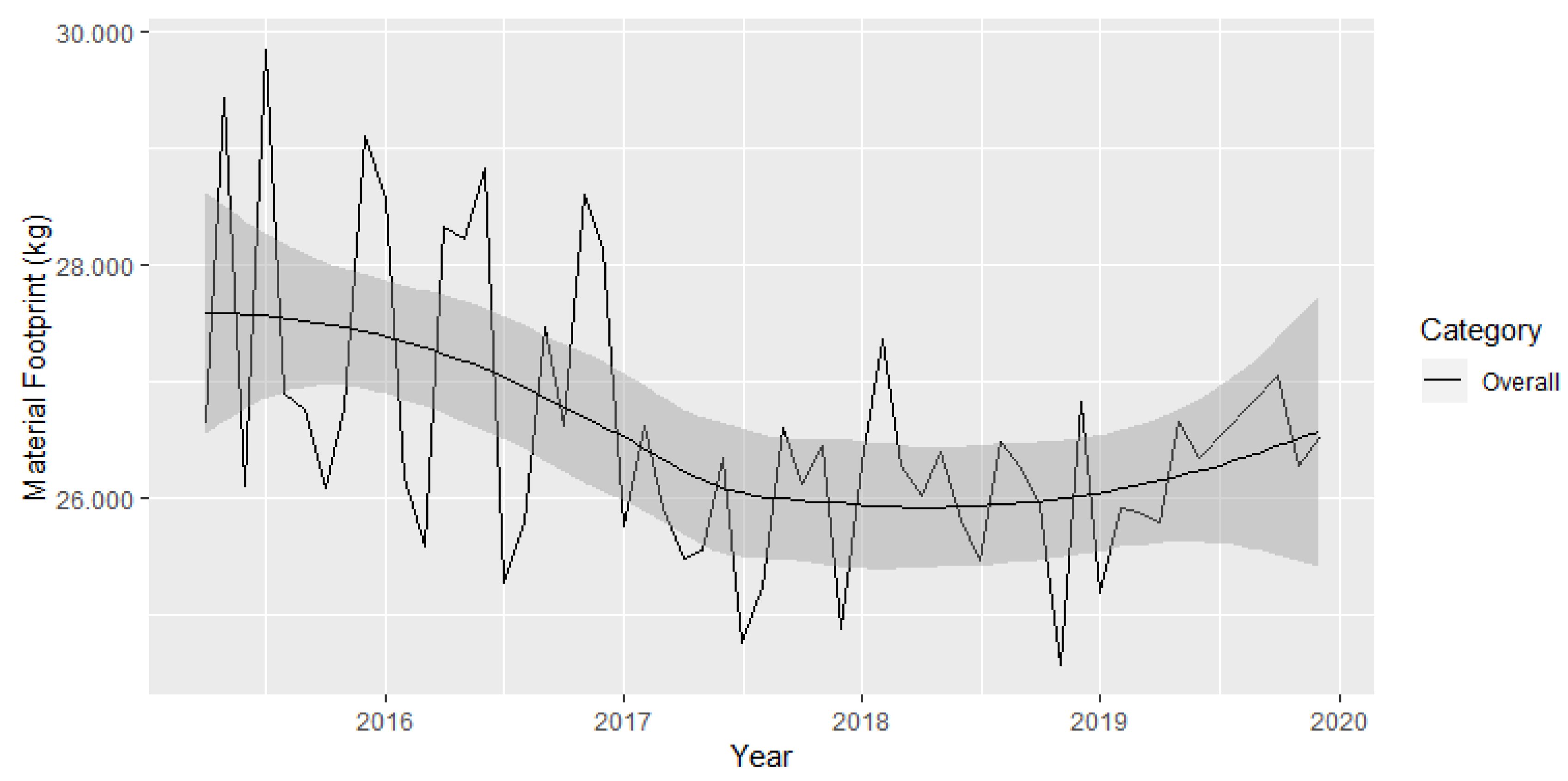
For a more detailed view of the Material Footprint in the past five years, we disaggregate the yearly observations into monthly observations. Figure 2 shows the monthly average overall Material Footprint between 2015 and 2019. Here, we can observe a greater variability between 2015 and 2017 than in the following year until 2019. At the start of the survey, the smaller confidence (at 95%) can be explained by smaller sample sizes at the beginning that increase the variance in the monthly mean Material Footprints. In this regard, the decreasing Material Footprints between 2015 and 2017 should be interpreted cautiously, considering the high variability in reported Material Footprints.
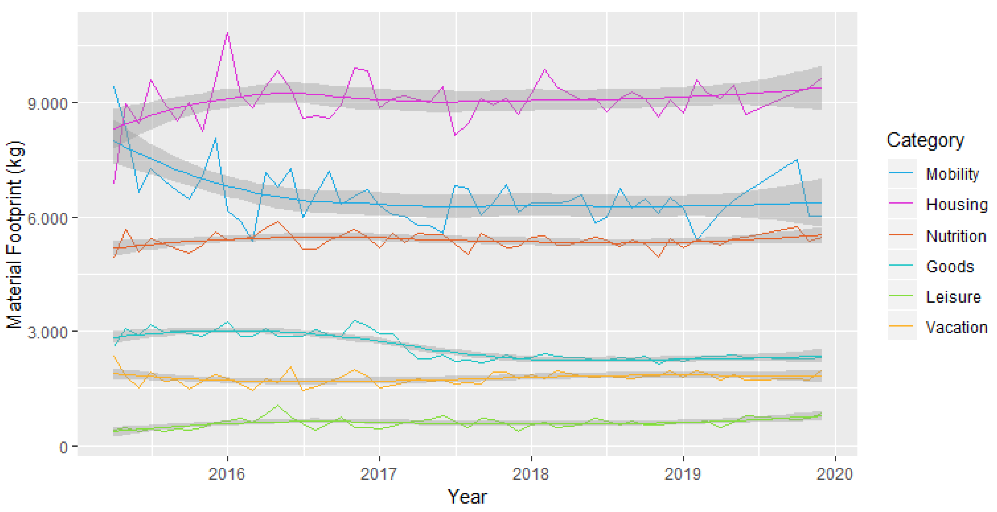
The same accounts for the Material Footprints along the consumption categories (Figure 3) showing a greater uncertainty in 2015 with decreasing Material Footprints of mobility and increasing footprints in housing. Figure 3 suggests a slight increase in housing Material Footprint since 2018, and a drop in the Material Footprint for consumer goods in 2017, while Material Footprints for leisure activities and vacations increase from 2017 onwards. Overall, the slight increasing and decreasing trends seem to cancel each other out, such that no relevant decreasing trend for the overall Material Footprint is observed between 2015 and 2019.

4.2. STL Predictions

In this section, we show the results of STL predictions of the overall Material Footprint as well as of housing, nutrition and mobility. We focus on the three major categories housing, nutrition and mobility since those categories effectively cover 91% of variation in the overall Material Footprint [15]. The predictions are used to forecast the Material Footprints of private consumption in the near future. Before, we report the prediction accuracy of the prediction models applied. Table 3 shows the forecast errors RMSE, MAE, MAPE and MASE for STL-ARIMA, STL-ETS for predicting the overall Material Footprint (MF) as well as in housing, nutrition and mobility.
The forecast MASE of the STL-ARIMA is lower than for a naïve forecast for all Material Footprint categories analysed, except mobility. The mean absolute percentage error (MAPE) is between 2.6% and 8.9%. The MAPE is lowest for the overall Material Footprint (2.6%) accordingly, showing the lowest MASE. The forecast error for the mobility Material Footprint is largest with a slightly more accurate forecast of the exponential smoothing (8.9%). Hence, we use STL-ARIMA predictions for the overall, housing and nutrition footprints and STL-ETS predictions for the mobility footprint. The MASE suggests that STL algorithms fit better than naïve forecasts with low prediction errors (MAPE). However, the prediction error in mobility is relatively high. The results should be interpreted accordingly. On average, the prediction of the Material Footprint in mobility is 8.9% off.
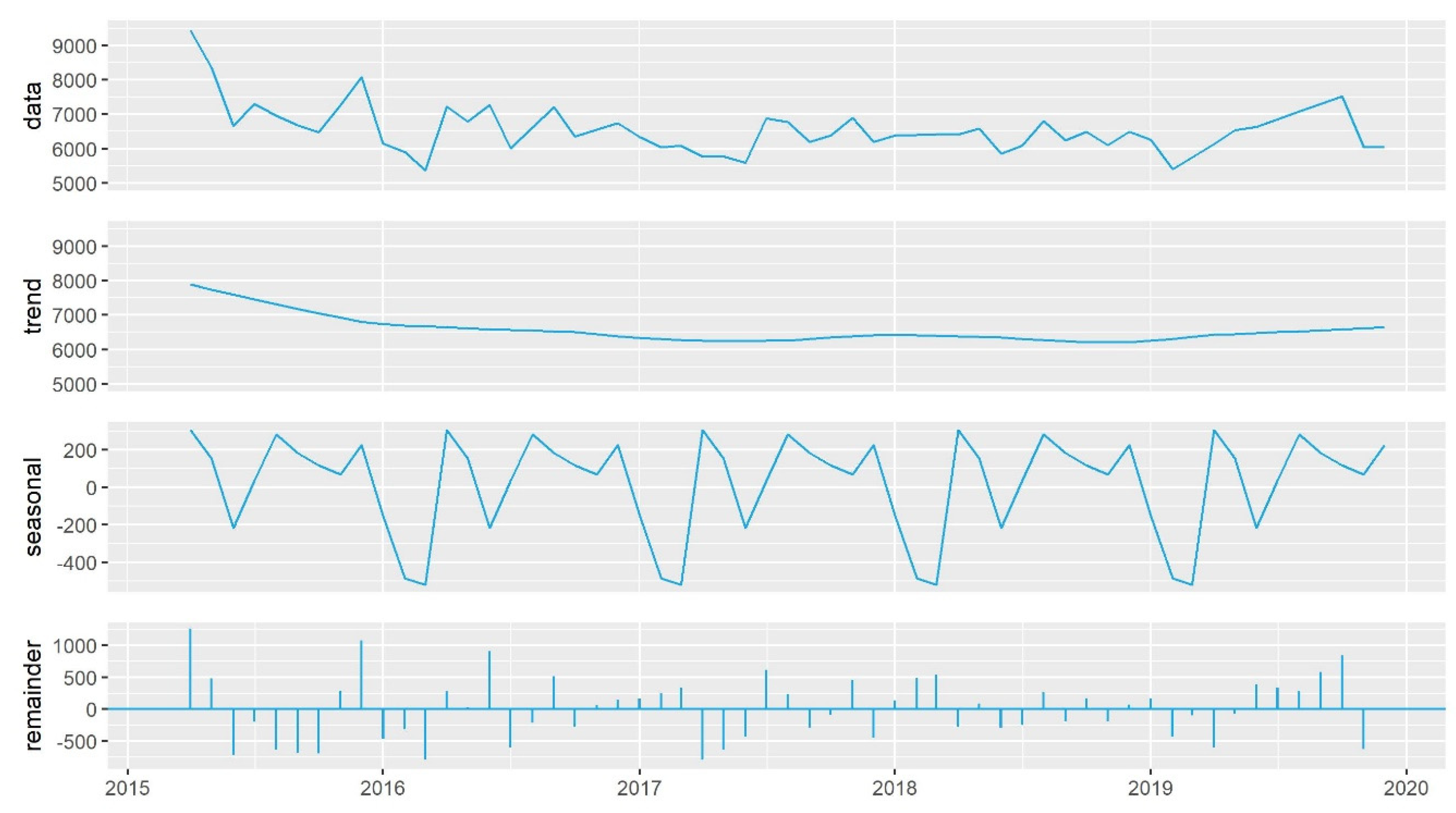
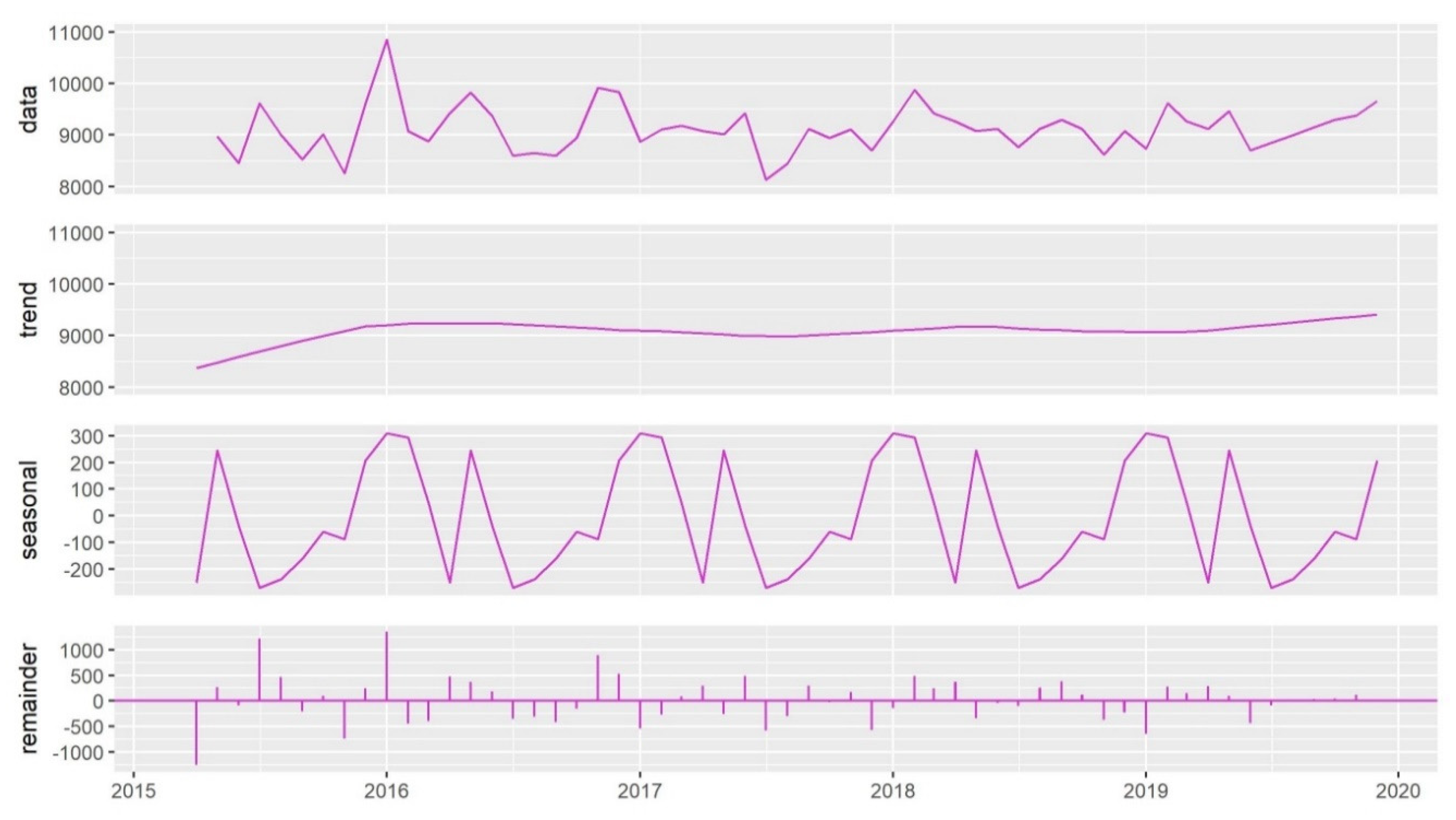
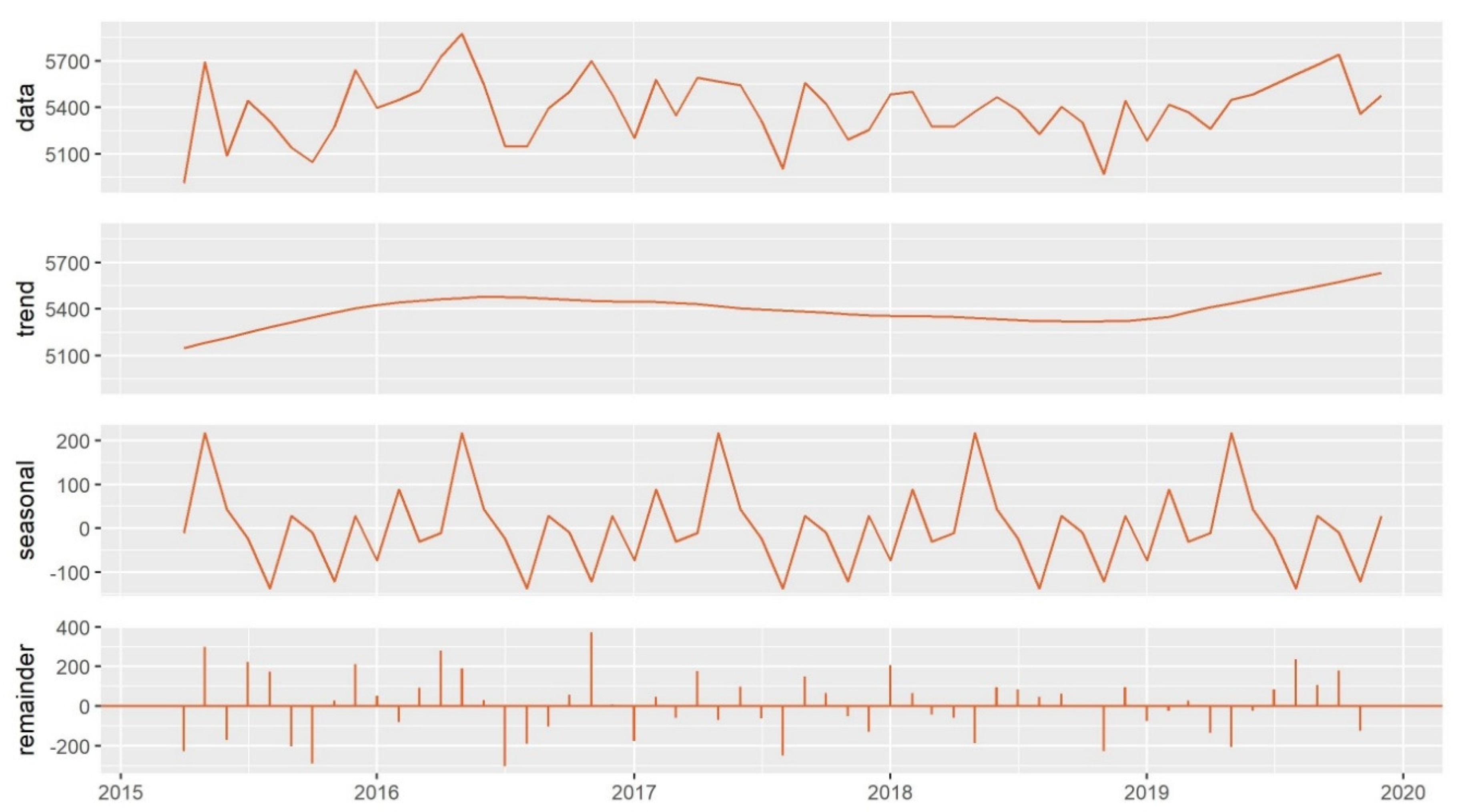
The seasonal and trend decomposition of the data allow us to depict the seasonal variation separately from the trend underlying the data. Figure 4 shows the decomposed time series of the overall Material Footprint and the remaining error that is not explained by the trend and seasonal component. The seasonal component shows that lower Material Footprints are recorded in the summer months. This may occur because respondents report higher Material Footprints in housing during winter due to higher heating and lower Material Footprints in mobility during summer due to holidays without commuting. The decomposed time series of the Material Footprint in housing, mobility and nutrition is presented in the Appendix A.
The overall Material Footprint shows a falling trend that increases again in the last year observed. Furthermore, the seasonal variation that underlies the data occurs repeatedly. The remaining variation in the data that is not explained by trend and seasonal patterns decreases as time increases.
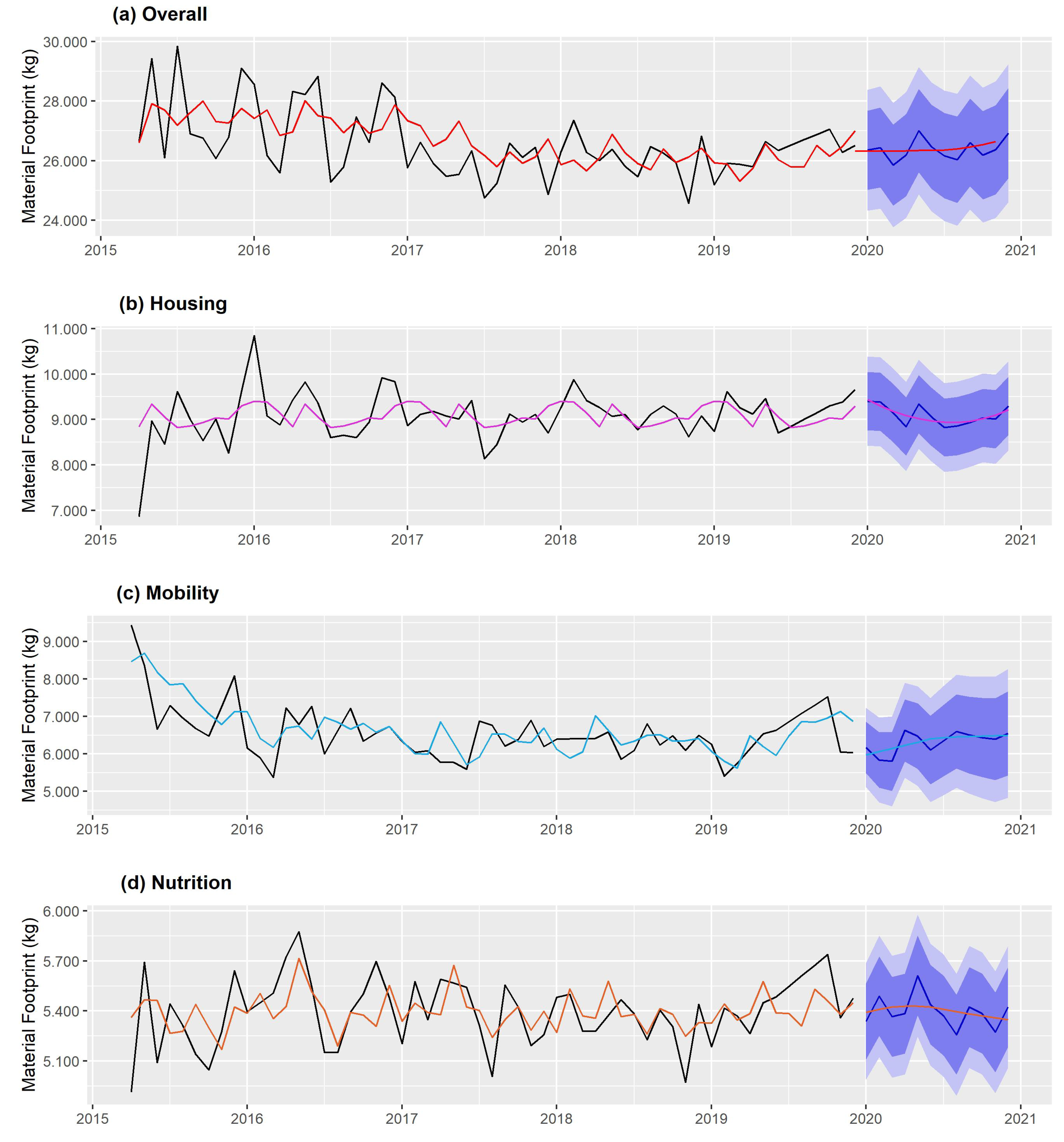
Figure 5 shows the observed Material Footprints and STL-ARIMA and STL-ETS predictions of the time series. The graph gives forecasts with confidence bands (85% and 90% level) for one year until December 2020 and a smoothing loess prediction of the forecast. The STL models fit the observed data well and follow the trend of the observed data. The relatively high forecast error does not result in misleading predictions. The STL-ARIMA prediction and forecast corroborates the findings from the time series analysis in Section 4.1. We predict no relevant changes in the Material Footprint between 2015 and 2020. The predictions and forecasts do not suggest relevant changes in the Material Footprint, but a relatively stable continuation of the Material Footprint of private consumption in Germany until 2020. However, there is a decrease in the overall Material Footprint and, more relevantly, the Material Footprint in relation to mobility. At the same time, we do find increasing Material Footprints for housing and nutrition.
As a result, the overall Material Footprint decreased by 2% between 2015 and 2020. Table 4 summarises the yearly changes in absolute and relative terms between 2015 and 2020. The yearly variability does suggest relevant changes in Material Footprint. For instance, the Material Footprint of mobility decreased in 2016 by 5.6% and in 2017 by −4.1%. However, on average, the Material Footprint of mobility decreased by only 2.3%. The Material Footprints of housing increased by 0.9% and of nutrition by 0.7% between 2015 and 2020. In comparison, an appropriate reduction path in order to meet a sustainable consumption of natural resources of 8t/cap in 2050 would suggest a (linear) reduction in the Material Footprint by more than 3.3% per year. Overall, the Material Footprint, on average, decreased by only 0.4% per year between 2015 and 2020. Consequently, our results show that the decrease in the Material Footprint in the past 5 years is insufficient and does not meet a sustainable reduction path.

5. Discussion and Conclusions

Recent research on the natural resource use of private consumption suggests a sustainable Material Footprint of 8 tons per capita by 2050. In 2016, Germany published its most recent editions of the National Program for Sustainable Consumption and German Resource Efficiency Program addressing consumer policies to reduce the private consumption of natural resources. Against this background, we analysed the population weighted data from the only Material Footprint calculator in Germany between 2015 and 2020. We analysed 113,559 user profiles and weighted the data according to population margins in Germany in order to give representative findings.
We found an overall Material Footprint of around 27 tons per capita in 2015 in Germany. Accordingly, the Material Footprint should follow a linear reduction of more than 3.3% per year in order to achieve sustainable resource use by 2050.
In order to test whether the Material Footprint of private consumption decreased accordingly over the past five years, we predict the Material Footprint of private consumption using a decomposed autoregressive (STL-ARIMA) and exponential smoothing (STL-ETS) algorithms. We showed that the STL-ARIMA and STL-ETS allows us to predict and forecast the Material Footprint more accurately than naïve forecasts with low prediction errors, reporting the observed trends reliably. Thus, the developed prediction models can be used to predict and forecast Material Footprint in upcoming studies. With more data available, the forecast can expand further into the future. Since our data, thus far, cover the past five years, we are only able to present a short-term forecast of one year ahead until the end of 2020. Our data do not allow for long-term forecasts. Rather, further research should focus on predicting trends in socio-economic features in order to deliver a more differentiated picture of who shows changes in Material Footprints and in which categories.
Our results for the overall Material Footprint as well as in housing, mobility and nutrition shows a relatively stable private resource use between 2015 and 2020. Housing, mobility and nutrition are by far the most important predictors of the material resource use of private households and explain more than 90% of the Material Footprint of private households.
We found an overall reduction of 2% in the past five years and an average reduction of 0.4% per year between 2015 and 2020 in Germany. Our results show that the Material Footprints in mobility are decreasing; however, they are still increasing for housing and nutrition. In housing, the Material Footprint increases by 0.9% per year on overage. The Material Footprint in mobility decreases relatively strongly, by 2.3% per year on average. In nutrition, the Material Footprint increases by 0.7% on average per year. We do not find that the Material Footprint of private consumption in Germany is following a sustainable reduction path.
Recent research suggests a sustainable Material Footprint of 8 tons per capita by the year 2050. This would have required an observed reduction of 3.3% per year. Our results thus suggest a reduction gap of 2.9 percentage points per year. However, our results show yearly decreases of up to 5.6% in mobility, suggesting a variability of resource use in private households that may allow us to quickly shift to sustainable reduction paths.
We conclude that the Material Footprint of private consumption in Germany is not decreasing sufficiently in order to achieve sustainable reductions.
Based on the study at hand, we suggest that policies on the consumption of natural resources in Germany should strengthen their efforts to support a decrease in natural resources by (1) identifying and incorporating reduction goals for the resource use of private consumption in national programs according to the scientific state of the art and (2) identifying the reduction potentials of different consumer policies in different consumption categories. In order to enable the monitoring of the Material Footprint of private consumption for specific policy evaluations, future works on predicting the Material Footprint of private households should further disaggregate the consumption categories. For instance, in terms of mobility, the Material Footprint over time could be further differentiated into mobility by car or public transport (e.g., local and long transport train) or air travel. In terms of housing, the Material Footprint should be further differentiated by the energy source of heating and electrical power supply (i.e., fossil fuels, renewable energies). Then, changes in the resource use over time in different consumption categories may be better linked to specific policies on reducing the resource use of private consumption, e.g., by supporting modal shifts. Predicting the Material Footprint developed on the basis of LCA data allows us to further disaggregate consumption categories in more detail for specific products and services. In this study, we developed a prediction model applicable to LCA data in order to monitor specific consumer policies addressing the resource use of private consumption in detail.

Author Contributions

Conceptualisation, J.B.; methodology, J.B.; software J.B., S.S.; validation, J.B.; formal analysis, J.B.; resources, C.L., K.B.; data curation, J.B., S.S.; writing—original draft preparation, J.B.; writing—review and editing, S.S., C.L.; visualisation, J.B.; supervision, C.L.; project administration, C.L.; funding acquisition, C.L. All authors have read and agreed to the published version of the manuscript.

Funding

This research received no external funding.

Conflicts of Interest

The authors declare no conflict of interest.

Appendix A

Figure A1. Seasonal and trend decomposition of the mobility Material Footprint.
Resources 09 00125 g0a1
Figure A2. Seasonal and trend decomposition of the housing Material Footprint.
Resources 09 00125 g0a2
Figure A3. Seasonal and trend decomposition of the nutrition Material Footprint.
Resources 09 00125 g0a3

References

  1. Bringezu, S.; Schütz, H.; Saurat, M.; Moll, S.; Acosta-Fernández, J.; Steger, S. Europe’s resource use. Basic trends, global and sectoral patterns and environmental and socioeconomic impacts. In Sustainable Resource Management: Global Trends, Visions and Policies; Bringezu, S., Bleischwitz, R., Eds.; Greenleaf Publishing: Sheffield, UK, 2009; pp. 52–154. [Google Scholar]
  2. Oberle, B.; Bringezu, S.; Hatfield-Dodds, S.; Hellweg, S.; Schandl, H.; Clement, J.; Cabernard, L.; Che, N.; Chen, D.; Droz-Georget, H.; et al. Report of the International Resource Panel. United Nations Environment Programme. In Global Resources Outlook 2019: Natural Resources for the Future We Want; Nairobi, Kenya, 2019; Available online: https://resourcepanel.org/reports/global-resources-outlook (accessed on 11 October 2020).
  3. Lettenmeier, M.; Liedtke, C.; Rohn, H. Eight Tons of Material Footprint—Suggestion for a Resource Cap for Household Consumption in Finland. Resources 2014, 3, 488–515. [Google Scholar] [CrossRef] [Green Version]
  4. Lettenmeier, M. A Sustainable Level of Material Footprint—Benchmark for Designing One-Planet Lifestyles Materiaalijalanjäljen kestävä taso –mittapuu yhden planeetan elämäntapojen toteuttamiseen; Aalto University: Helsinki, Finland, 2018. [Google Scholar]
  5. Bringezu, S. Possible target corridor for sustainable use of global material resources. Resources 2015, 4, 25–54. [Google Scholar] [CrossRef]
  6. Bringezu, S. Toward Science-Based and Knowledge-Based Targets for Global Sustainable Resource Use. Resources 2019, 8, 140. [Google Scholar] [CrossRef] [Green Version]
  7. German Federal Government. Die Deutsche Nachhaltigkeitsstrategie 2016—Der Weg in eine enkelgerechte Zukunft; German Federal Government: Frankfurt am Main, Germany, 2016.
  8. UN. Transforming Our World: The 2030 Agenda for Sustainable Development. 2015. Available online: https://sustainabledevelopment.un.org/content/documents/21252030%20Agenda%20for%20Sustainable%20Development%20web.pdf (accessed on 18 April 2018).
  9. Domenech, T.; Bahn-Walkowiak, B. Transition towards a resource efficient circular economy in Europe: Policy lessons from the EU and the member states. Ecol. Econ. 2019, 155, 7–19. [Google Scholar] [CrossRef]
  10. German Federal Ministry for the Environment, Nature Conservation and Nuclear Safety (BMU 2016). German Resource Efficiency Programme II Programme for the Sustainable Use and Conservation of Natural Resources Adopted by the Federal Cabinet on 2 March 2016. 2016. Available online: https://www.bmu.de/fileadmin/Daten_BMU/Pools/Broschueren/german_resource_efficiency_programme_ii_bf.pdf (accessed on 11 October 2020).
  11. German Federal Statistical Office (Destatis). Umweltökonomische Gesamtrechnung. Nachhaltige Entwicklung in Deutschland Indikatoren zu Umwelt und Ökonomie, Bericht 2016; German Federal Statistical Office: Wiesbaden, Germany, 2016.
  12. German Federal Ministry for the Environment, Nature Conservation and Nuclear Safety (BMU 2017). Nationales Programm für nachhaltigen Konsum. Gesellschaftlicher Wandel durch einen nachhaltigen Lebensstil. Available online: http://www.bmu.de/fileadmin/Daten_BMU/Pools/Broschueren/nachhaltiger_konsum_broschuere_bf.pdf (accessed on 19 April 2018).
  13. Lettenmeier, M.; Rohn, H.; Liedtke, C.; Schmidt-Bleek, F. Resource Productivity in 7Steps—How to Develop Eco-Innovative Products and Services and Improve Their Material Footprint. Wuppertal Spezial 41; Wuppertal Institute for Climate, Environment and Energy: Wuppertal, Germany, 2009. [Google Scholar]
  14. Buhl, J.; Liedtke, C.; Teubler, J.; Bienge, K.; Schmidt, N. Measure or Management?—Resource Use Indicators for Policymakers Based on Microdata by Households. Sustainability 2018, 10, 4467. [Google Scholar] [CrossRef] [Green Version]
  15. Buhl, J.; Liedtke, C.; Teubler, J.; Schuster, S.; Bienge, K. A material footprint model for green information systems–using statistical learning to identify the predictors of natural resource use. Cogent. Eng. 2019, 6, 1616655. [Google Scholar] [CrossRef]
  16. Buhl, J.; Liedtke, C.; Teubler, J.; Bienge, K. The Material Footprint of private households in Germany: Linking the natural resource use and socioeconomic characteristics of users from an online footprint calculator in Germany. Sustain. Prod. Consum. 2019, 20, 74–83. [Google Scholar] [CrossRef]
  17. Schmidt-Bleek, F. The Earth: Natural Resources and Human Intervention; Haus Publishing: London, UK, 2009. [Google Scholar]
  18. Liedtke, C.; Bienge, K.; Wiesen, K.; Teubler, J.; Greiff, K.; Lettenmeier, M.; Rohn, H. Resource Use in the Production and Consumption System—The MIPS Approach. Resources 2014, 3, 544–574. [Google Scholar] [CrossRef] [Green Version]
  19. Wiesen, K.; Saurat, M.; Lettenmeier, M. Calculating the Material Input per Service Unit using the Ecoinvent Database. Int. J. Perform. Eng. 2014, 10, 357–366. [Google Scholar]
  20. Wiesen, K.; Wirges, M. From cumulated energy demand to cumulated raw material demand: The material footprint as a sum parameter in life cycle assessment. Energy Sustain. Soc. 2017, 7, 13. [Google Scholar] [CrossRef]
  21. Teubler, J.; Buhl, J.; Lettenmeier, M.; Greiff, K.; Liedtke, C. A Household’s Burden–The Embodied Resource Use of Household Equipment in Germany. Ecol. Econ. 2018, 146, 96–105. [Google Scholar] [CrossRef] [Green Version]
  22. Greiff, K.; Teubler, J.; Baedeker, C.; Liedtke, C.; Rohn, H. Material and Carbon Footprint of Household Activities. In Living Labs: Design and Assessment of Sustainable Living; Keyson, D.V., Guerra-Santin, O., Lockton, D., Eds.; Springer International Publishing: Cham, Switzerland, 2017; pp. 259–275. [Google Scholar]
  23. Wiedmann, T.O.; Schandl, H.; Lenzen, M.; Moran, D.; Suh, S.; West, J.; Kanemoto, K. The material footprint of nations. Proc. Natl. Acad. Sci. USA 2015, 112, 6271–6276. [Google Scholar] [CrossRef] [Green Version]
  24. Giljum, S.; Bruckner, M.; Martinez, A. Material Footprint Assessment in a Global Input-Output Framework. J. Ind. Ecol. 2015, 19, 792–804. [Google Scholar] [CrossRef] [Green Version]
  25. Lutter, S.; Giljum, S.; Bruckner, M. A review and comparative assessment of existing approaches to calculate material footprints. Ecol. Econ. 2016, 127, 1–10. [Google Scholar] [CrossRef] [Green Version]
  26. Buhl, J. Revisiting rebound effects from material resource use. Indications for Germany considering social heterogeneity. Resources 2014, 3, 106–122. [Google Scholar] [CrossRef] [Green Version]
  27. Buhl, J.; Teubler, J.; Liedtke, C.; Stadler, K. Ressourcenverbrauch private Haushalte NRW—Explorative Analyse. Final report of the funded project “Konzeptionelle Analysen und Überlegungen zur Ausgestaltung einer Nachhaltigkeitsstrategie aus wissenschaftlicher Sicht“ for the State Agency for Nature, Environment and Consumer Protection NRW (LANUV); Wuppertal Institute for Climate, Environment and Energy: Wuppertal, Germany, 2016. [Google Scholar]
  28. Buhl, J.; Acosta, J. Work less, do less? Working time reductions and rebound effects. Sustain. Sci. 2016, 11, 261–267. [Google Scholar] [CrossRef]
  29. Buhl, J.; Acosta, J. Indirect effects from resource sufficiency behaviour. In Rethinking Climate and Energy Policies. New Perspectives on the Rebound Phenomenon; Santarius, T., Walnum, H.J., Aall, C., Eds.; Springer: New York, NY, USA, 2016; pp. 37–55. [Google Scholar]
  30. Buhl, J.; Teubler, J.; Liedtke, C.; Stadler, K. Der Ressourcenverbrauch privater Haushalte in NRW—The resource use of private households in North Rhine-Westphalia, Germany. Uwf UmweltWirtschaftsForum Sustain. Manag. Forum 2017, 25, 255–264. [Google Scholar]
  31. Buhl, J.; Liedtke, C.; Bienge, K. How Much Environment Do Humans Need? Evidence from an Integrated Online User Application Linking Natural Resource Use and Subjective Well-Being in Germany. Resources 2017, 6, 67. [Google Scholar] [CrossRef] [Green Version]
  32. Gill, B.; Moeller, S. GHG emissions and the rural-urban divide. A carbon footprint analysis based on the German official income and expenditure survey. Ecol. Econ. 2018, 145, 160–169. [Google Scholar] [CrossRef]
  33. Junnila, S.; Ottelin, J.; Leinikka, L. Influence of Reduced Ownership on the Environmental Benefits of the Circular Economy. Sustainability 2018, 10, 4077. [Google Scholar] [CrossRef] [Green Version]
  34. Ottelin, J.; Heinonen, J.; Junnila, S. Carbon and material footprints of a welfare state: Why and how governments should enhance green investments. Environ. Sci. Policy 2018, 86, 1–10. [Google Scholar] [CrossRef]
  35. Pothen, F.; Reaños, T.; Angel, M. The distribution of material footprints in Germany (No. 18-022). Ecol. Econ. 2018, 153, 237–251. [Google Scholar] [CrossRef] [Green Version]
  36. German Federal Statistical Office and the Statistical Offices of the Länder. Population Depending on Age (Eleven Classes of Years) and Sex; Bayerisches Landesamt für Statistik: Fürth, Germany, 2014.
  37. Pasek, J.; DeBell, M.; Krosnick, J.A. Standardizing and Democratizing Survey Weights: The ANES Weighting System and Anesrake. 2014. Available online: https://surveyinsights.org/wp-content/uploads/2014/07/Full-anesrake-paper.pdf (accessed on 11 October 2020).
  38. Shao, Z.; Chao, F.; Yang, S.-L.; Zhou, K.-L. A review of the decomposition methodology for extracting and identifying the fluctuation characteristics in electricity demand forecasting. Renew. Sust. Energy Rev. 2017, 75, 123–136. [Google Scholar] [CrossRef]
  39. De Oliveira, E.M.; Oliveira, F.L.C. Forecasting mid-long term electric energy consumption through bagging ARIMA and exponential smoothing methods. Energy 2018, 144, 776–788. [Google Scholar] [CrossRef]
  40. Fatima, S.; Ali, S.S.; Zia, S.S.; Hussain, E.; Fraz, T.R.; Khan, M.S. Forecasting carbon dioxide emission of Asian countries using ARIMA and simple exponential smoothing models. Int. J. Econ. Environ. Geol. 2019, 10, 64–69. [Google Scholar] [CrossRef]
  41. Hyndman, R.J.; Khandakar, Y. Automatic Time Series for Forecasting: The Forecast Package for R (No. 6/07); Department of Econometrics and Business Statistics, Monash University: Clayton, VIC, Australia, 2007. [Google Scholar]
  42. Hylleberg, S.; Engle, R.; Granger, C.; Yoo, B. Seasonal integration and cointegra-tion. J. Econom. 1990, 44, 215–238. [Google Scholar] [CrossRef]
  43. Kwiatkowski, D.; Phillips, P.C.; Schmidt, P.; Shin, Y. Testing the null hypothesisof statioanrity against the alternative of a unit root. J. Econom. 1992, 54, 159–178. [Google Scholar] [CrossRef]
  44. Hyndman, R.J.; Athanasopoulos, G. Forecasting: Principles and Practice; OTexts: Melbourne, Australia, 2018. [Google Scholar]
  45. Cleveland, R.B.; Cleveland, W.S.; McRae, J.E.; Terpenning, I. STL: A seasonal-trend decomposition. J. Off. Stat. 1990, 6, 3–73. [Google Scholar]
  46. Hyndman, R.J. Measuring Forecast Accuracy. In Business Forecasting: Practical Problems and Solutions; Gilliland, M., Tashman, L., Sglavo, U., Eds.; John Wiley & Sons: New York, NY, USA, 2016; pp. 177–183. [Google Scholar]
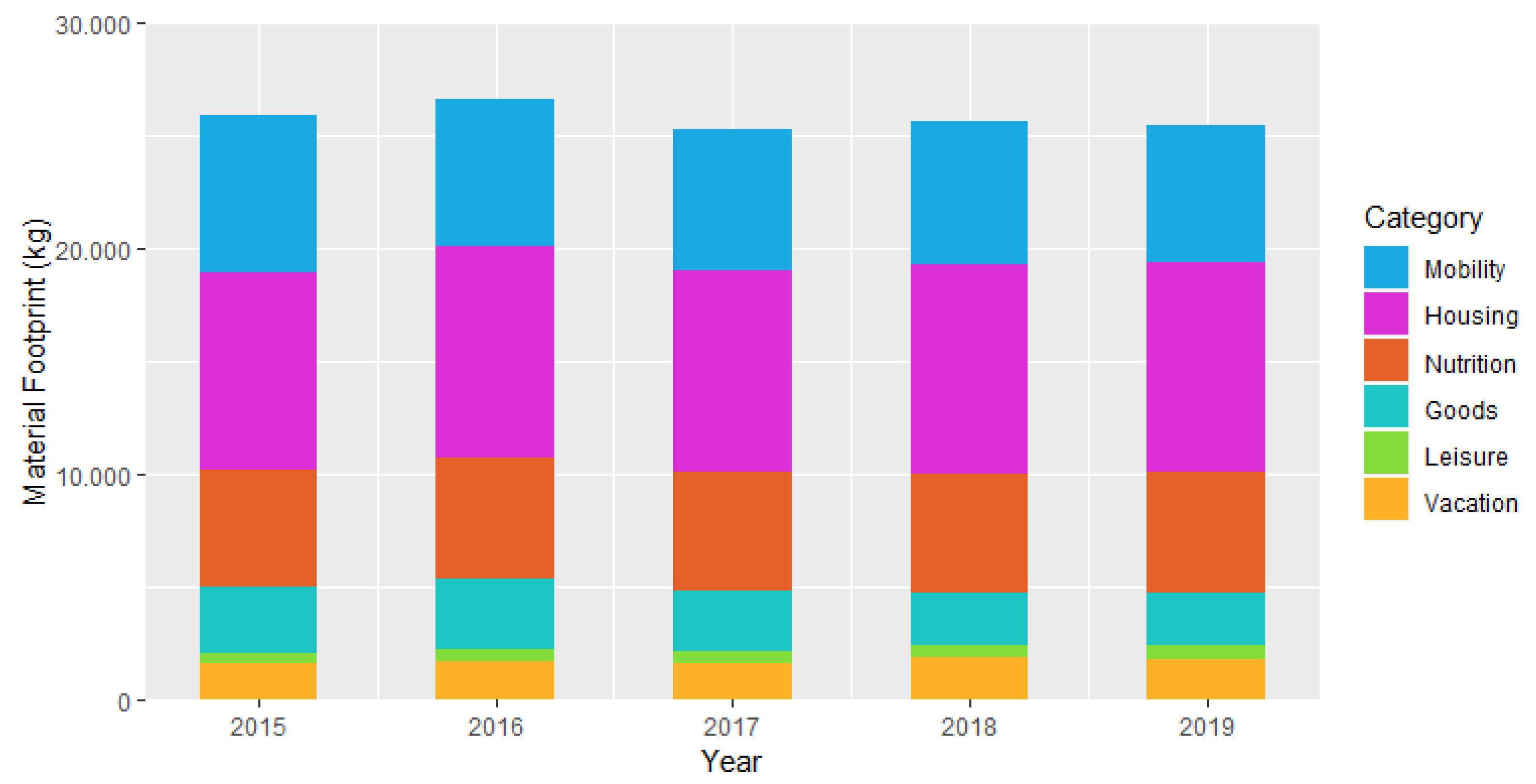
Figure 1. The mean Material Footprint of private households between 2015 and 2019 in Germany.
Resources 09 00125 g001
Figure 2. The monthly mean Material Footprint between 2015 and 2019 in Germany, with 95% confidence band around locally weighted estimations (loess).
Resources 09 00125 g002
Figure 3. The monthly mean Material Footprint between 2015 and 2019 in Germany by consumption category, with 95% confidence band around locally weighted estimations (loess).
Resources 09 00125 g003
Figure 4. Seasonal and trend decomposition of the overall Material Footprint (in kg) in Germany between 2015 and 2019: ‘data’ gives the monthly observed data; ‘trend’ gives the overall trend; ‘seasonal’ gives the seasonal trend and ‘remainder’ gives the remaining error not explained by an overall or seasonal trend.
Resources 09 00125 g004
Figure 5. Season–trend decomposition using loess (STL) predictions and forecasts of the Material Footprint (a) overall and of (b) housing, (c) mobility, (d) nutrition in Germany between 2015 and 2020. The red line gives the predictions, the black line the observed and forecasted data. The forecasted data are reported with 85 (dark blue) and 90% (light blue) confidence bands.
Resources 09 00125 g005
Table 1. Descriptive statistics * of the Material Footprint and selected characteristics of users.
VariableValid.nMeansdMinMax
Overall (kg)113,55925,710.889882.72271174,243
Housing (kg)113,5118876.414109.294528,638
Mobility (kg)113,5776472.456332.86039,484
Nutrition (kg)113,5845212.581364419505
Goods (kg)113,5522476.211092.7406653
Vacation (kg)113,5491642.941552.6808790
Leisure (kg)113,630534.54781.9507328
Age (years)62,91734.1514.06188
Female (ref. male)63,3140.630.4801
* Descriptive statistics include the valid number of observations (valid.n), the mean, the standard deviation (sd), the minimum (min) and maximum (max).
Table 2. Shares of sex and age groups (in years) in observed, census and weighted data.
SampleMaleFemale<1818–2525–3030–4040–5050–6565–75>75
Observed0.370.630.100.180.170.250.140.140.020.01
Census *0.490.510.160.080.060.120.170.200.110.09
Weighted0.490.510.180.090.070.130.180.220.110.03
* Data from the latest national census in Germany in 2011.
Table 3. Forecast error of the seasonally decomposed autoregressive (STL-ARIMA) and exponential smoothing (STL-ETS) predictions of the Material Footprint overall and of housing, mobility, nutrition between 2015 and 2020.
Material FootprintOverallHousingMobilityNutrition
ModelSTL-ARIMASTL-ETSSTL-ARIMASTL-ETSSTL-ARIMASTL-ETSSTL-ARIMASTL-ETS
RMSE8491366385385719710210216
MAE6861215330331607599154161
MAPE2.64.63.63.69.08.92.83.0
MASE0.510.90.580.580.940.920.60.63
Table 4. Mean yearly Material Footprints (in kg) overall and of housing, mobility, nutrition and yearly relative changes (in %) between 2015 and 2020.
Material FootprintOverall
(in kg)
Overall
(in %)
Housing
(in kg)
Housing
(in %)
Mobility
(in kg)
Mobility
(in %)
Nutrition
(in kg)
Nutrition
(in %)
201526,912-8743-6963-5213-
201627,2151.1293106.486575−5.6054213.99
201725,796−5.218921−4.186304−4.105289−2.43
201826,1551.3992133.2763841.3053140.47
201925,985−0.6592530.446065−5.0053510.69
202026,3811.539094−1.7263214.2053970.86
Publisher’s Note: MDPI stays neutral with regard to jurisdictional claims in published maps and institutional affiliations.