Article

Life Cycle Assessment of Oyster Farming in the Po Delta, Northern Italy

1
Department of Life Sciences and Biotechnology, University of Ferrara, Via L. Borsari 46, 44121 Ferrara, Italy
2
Istituto Delta Ecologia Applicata, Via B. Bartok 29, 44124 Ferrara, Italy
*
Author to whom correspondence should be addressed.
Resources 2019, 8(4), 170; https://doi.org/10.3390/resources8040170
Submission received: 14 August 2019 / Revised: 10 October 2019 / Accepted: 25 October 2019 / Published: 30 October 2019

Abstract

:
Oysters represent an important portion of the world’s total aquaculture production. In recent years, in Italy, oyster farming has progressively increased its role in the economic growth of the aquaculture sector and still has great potential for growth. As in any other production, oyster farming generates environmental impacts over an oyster’s life cycle, due to material, energy, fuel, and water use. The aim of this work was to carry out a cradle-to-gate life cycle assessment (LCA) of 1 kg of fresh oysters of commercial size produced in the Po delta area, northern Italy. Two scenarios were considered. The current scenario provides for oyster seed purchasing from France and transport to Italy, whereas the alternative scenario includes in situ seed production in order to realize a complete local and traceable supply chain. Eco-indicator® 99-H and ReCiPe® midpoint (H) v.1.12 were used to perform the impact assessments. The overall impacts of the two scenarios were very similar and indicated that the main hotspots were the fattening and prefattening phases of farming, which were common in both scenarios. Focusing the analysis on the first stages, transport from France had a greater impact than did local seed production, emphasizing the importance of a short supply chain in aquaculture production.

1. Introduction

Assuring appropriate food and nutrition security worldwide is a daunting challenge [1]. A fundamental issue for future development is if it is possible to obtain a food supply for a human population that is expected to exceed 9 billion by 2050 [2]. Undoubtedly, advances have been made in hunger decline, but often at the expense of the environment and placing large pressures on nature [3]. Direct and indirect land use effects, freshwater scarcity, deforestation, and biodiversity reduction are contributing to a general loss of sustainability and a reduced capacity to leave the same food supply opportunities for future generations [4]. Under this scenario, fisheries and aquaculture, the food industries that need to use soil and freshwater less [5], will be one of the greatest resources in supporting human nutrition for the next years [6]. Aquaculture contributes about 171 × 106 tons per year, about 2% of total food production, and supplies more than 15% of the total protein consumed [7]. Since the 1990s, many fish stocks have been overexploited [8], and catches are still above a level of sustainability [9]. In contrast, for the past five decades, the aquaculture sector has been increasing at a constant rate, now accounting for about 50% of all fishery products [7]: at a level of growth of about 5.8% per year, this overshoots both the population growth rate (1.07% per year) [7] and the food produced by agriculture (<2.0% per year) [10].
Shellfish, in particular, are becoming of growing importance, with 22% of the overall world aquaculture production [11]. Even though East Asia largely dominates the global harvest, the EU is gaining significantly in oyster (Crassostrea gigas and Ostrea edulis), mussel (Mytilus edulis and Mitilus galloprovincialis), and clam (Ruditapes spp.) production [12]. Besides production volume, mollusks could be a potential key resource, because on the one hand, they provide a highly nutritious and protein-rich food, and on the other hand, they do not require additional feed or freshwater input (as, for example, fish and crustaceans do) and only need simple and low-energy-eater culture technologies [13]. Moreover, mollusk culture can provide several ecosystem services to the surrounding environment, including water quality preservation, coastal maintenance, seabed settling, and nutrient cycling and sequestration [14]. It can be said that shelled mollusk aquaculture can be recommended as one of the more sustainable and low-impact “food sources of the future” [15].
Indeed, France is the EU leader for oyster production (about 125,000 tons per year), Spain for mussels (about 209,000 tons per year), and Italy for clams (about 32,000 tons per year) [16]. Even though oyster farming was born on the Italian peninsula and was performed by the Romans in the first century BC [17], only recently has Italy invested in oyster farming to meet an increasing consumer demand, with an increased production of about 300% in a few years [18]. In fact, despite the minimal Italian production of oysters, consumers increasingly value their particular taste, making this a very promising and highly valuable sector [19].
For a better understanding of the potential of market expansion and the environmental concerns about mollusk aquaculture, life cycle assessments (LCAs) have been more frequently used to draw out best practices and to calculate the environmental impact of products and process [20]. A LCA is an International Organization for Standardization (ISO)-standardized accounting framework used to develop a “cradle-to-grave” assessment of the potential environmental impacts deriving from the use of energy, water, and material inputs [21]. While LCAs in the agriculture sector are relatively well established [22,23], the application of this tool for evaluating aquaculture production systems is a more recent phenomenon [24]. To date, LCA researchers have examined fish products [25,26,27,28] and shelled mollusks (mussels) [29,30]. The studies have suggested that LCAs could be appropriate to evaluate eco-friendliness and the environmental impacts of seafood products. Oysters already account for more than 30% of the overall production of mollusks worldwide, and they are therefore relevant for the whole seafood sector [31], but to the best of the authors’ knowledge, besides a report published by the Scottish Aquaculture Research Forum on the carbon footprint of Scottish oyster farming [32], only one unique paper has been published in the international literature that has applied an LCA to oyster farming in Brazil [33]. In 2016, the Italian production of oysters was assessed at a level of about 6300 tons [34], using almost exclusively oyster seeds supplied from abroad, France in particular. A few attempts have been recently performed to set up an in-house hatchery, with promising results [35].
This study was principally aimed at providing the first attempt to evaluate the environmental impacts of Italian oyster farming, from seed hatching to final packaging for the market, comparing the two upstream phases of purchasing seeds from France or producing seeds in a local hatchery. Moreover, the analysis was focused on an identification of the main hotspots of the supply chain in order to encourage the implementation of completely local sustainable production.

2. Materials and Methods

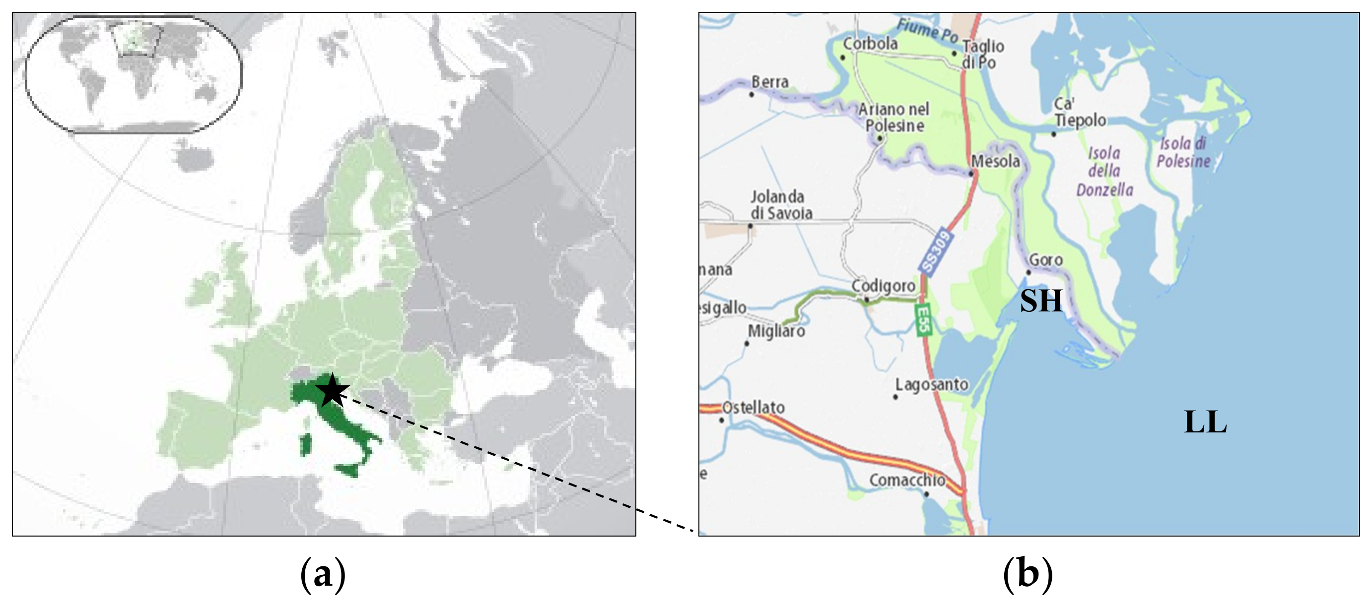
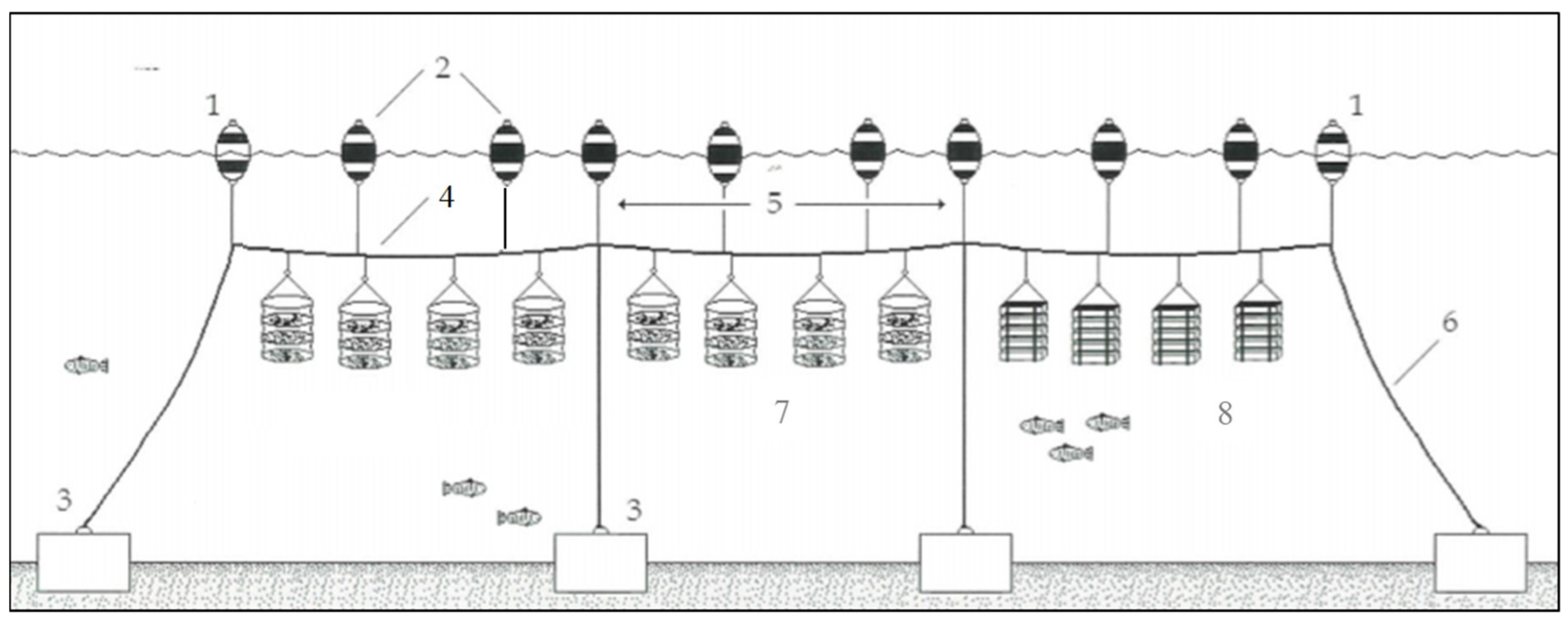
2.1. Description of the Case Study

The cultivation plant is located in Goro, in the Po river delta on the northeastern coast of Italy within the 3-mile zone from the coast under offshore conditions from the Adriatic Sea (Figure 1). It was developed in the last 4–5 years and produces about 10% of the oysters (Crassostrea gigas) farmed in Italy (8–10 tons/year).
Crassostrea gigas originates from the Atlantic Ocean and was introduced decades ago to the Adriatic coast for aquaculture scope. The breeding cycle starts with a phase of oyster prefattening (from about 10 to 30 mm long, 4 months), after which comes fattening (from 30 to 70–80 mm long, 8 months). Both prefattening and fattening are carried out in a long-line plant (Figure 2). Oyster farming lasts 12 months, and including in situ seed production, farming takes 16 months, from July/August to November of the following year.
A long-line plant is set up with a number of vertical ropes connected to a floating system, which is kept in suspension with emerging buoys. The system is maintained anchored to the seabed by concrete blocks (1200-kg anchoring blocks). Oysters are cultured in vertically stacked, multistory baskets composed of five plastic trays (40 cm in diameter, 10 cm of height) placed one on top of the other and fixed on the flotation system. Mooring lines and ropes keep the unit attached to each concrete block. Each unit measures about 800 m for a total of 3 parallel units 5 m from each other. The overall sea occupation is about 120,000 m2. To permit the correct water flow through the grids and for the adequate growth of mollusks, during the farming, trays and baskets are regularly checked to detach any clogging.
For the current scenario, oyster seeds were purchased at L’Epine (Ile de Noirmountier, France), 1596 km from Goro. For the alternative scenario, there was the opportunity to set up an in situ nursing and hatching phase to realize a complete local supply chain (excluding the contribution of French seeds). After end-fattening, mature oysters were harvested, selected, and packaged for market, with an average production loss of about 50%.
The number of seeds in both scenarios was about 200,000 spats, for a final production of about 100,000 oysters of commercial size (about 8 tons/year), corresponding to the annual production of the farm.

2.2. The LCA Framework

In an LCA, all consumed resources and emissions to the environment at all stages of the life cycle of a product or a process within specific boundaries are accounted for and evaluated, generally from the extraction of raw material to various end-of-life scenarios (i.e., waste, reuse, and recycling). An LCA consists of four stages: (1) the definition of the objective and scope; (2) a life cycle inventory; (3) an impact assessment; and (4) an interpretation of the results. Such an analysis allows for the management of the most important impacts throughout the entire product’s life cycle.

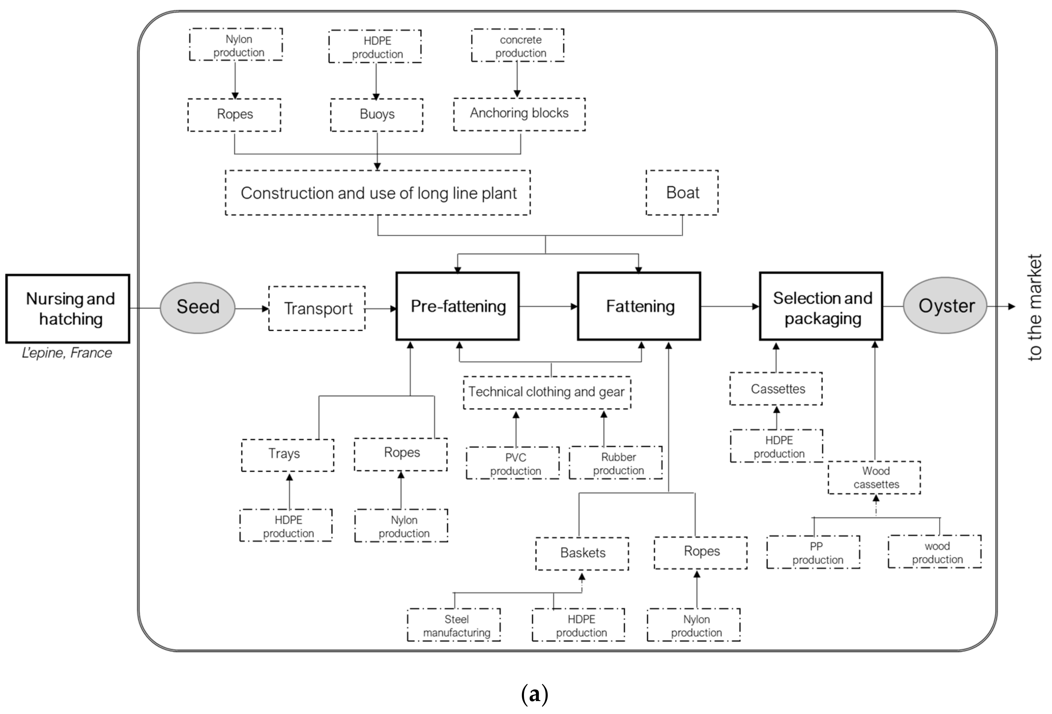
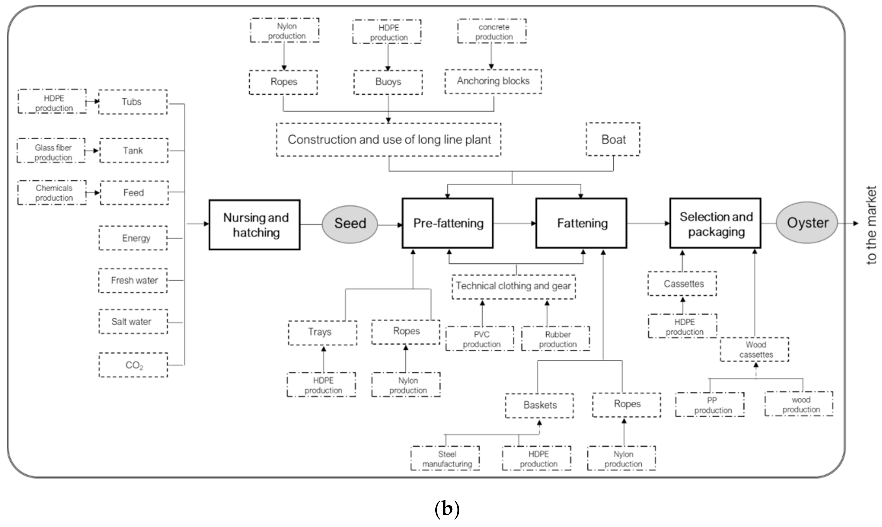
2.2.1. Goal and Scope Definition

The first step of an LCA is to define the goal and the scope. The aim of this study was to calculate the potential environmental impacts associated with oyster farming from seed to commercial size. In particular, the following aims were pursued:
-
Identification of the main hotspots existing under the current farming conditions described above; and
-
Comparison of the current scenario of oyster seed supply from France to an alternative in situ hatching.
The target audiences of this study are the stakeholders of the oyster industry sector, policy-makers, and those involved in LCAs and aquaculture.
The process within the system boundaries for the two scenarios and the main flows for oyster farming are summarized in Figure 3. Both scenarios share four stages: (1) the nursing and hatching of seed; (2) the prefattening of seeds; (3) fattening; and (4) selection and packaging. The second scenario provides for completely local farming, including in situ stage 1.
A supplier gate-to-gate assessment was applied in the first scenario because data on nursing and hatching in L’Epine were not available (including the transport of seed to Goro). A cradle-to-gate assessment was performed in the alternative scenario, including all energy and material inputs used to produce spats. It is worthwhile to specify that the construction of local nursing and hatching buildings was excluded from the impact calculations because they already exist and have been used for other activities in aquaculture for decades. Similarly, oyster waste was not included, because it is usually thrown back into the sea. The possible valorization of oyster waste or oyster shells is beyond the scope of this article.
A functional unit (FU) is defined by ISO standards as a quantified performance of a product system and is used as a reference unit from which all environmental impacts are quantified. The FU chosen for the assessment of oyster farming was 12 oysters at farm gate, which corresponded to 1 kg of commercial fresh oysters for market. This farm gate measure was the FU used in de Alvarenga et al. [33].

2.2.2. Life Cycle Inventory

Data for an assessment of seed production, oyster cultivation, selection, and packaging were gathered in 2019 based on the personal experiences of the authors and interviews with local oyster farmers (Table 1), and these are referred to as the average of the last 5 years of production.
The off-shore long-line plant was accessed with a wooden barge (10 m) specifically used for oyster culturing. The overall number of boat runs offshore for checking and harvesting activities is about 110 per year, 30 for prefattening and 80 for fattening, using diesel as fuel. The ropes are made of nylon, and HDPE (High Density Polyethylene) is the main component of trays, baskets, buoys, and tanks. HDPE tanks and tubs are completely recyclable, whereas HDPE buoys, baskets, and trays are waste after use because of the accumulation of organic fouling. Technical clothing consists of PVC (Polyvinyl chloride) diving vests, rubber gloves, and boots.
The life spans of materials are 15 years for HPDE tubs and the glass fiber tanks used in seed production; 8 years for buoys, ropes, trays, and baskets; and 3 months to 2 years for clothing and gears. Boat and long-line plant life was estimated at 30 and 50 years, respectively. When possible, the end-of-life scenario of complete recycling was considered for plastics.
Electricity consumption is caused by seawater pumps and by the equipment inside the building where nursing and hatching are carried out. The yearly amount of fuel and electricity consumption was estimated based on data provided by farmers relative to the year 2018. The electricity is provided by a PV (photovoltaic) plant already installed in the building. In addition, 100 L of nutrient broth is necessary for seed feeding (freshwater solution of salts and vitamins) [36].
CO2 is supplied using a loaded/empty mode, so the impact of cylinders was neglected. On the other hand, background processes and raw material/electricity production were taken into account through the use of the Ecoinvent 3.6® database (Zurich, Switzerland) [37]. The estimated distance from L’Epine to Goro was assumed to be covered by a 16–32 tons Euro-5 refrigerated truck. The total (inputs and outputs) background process requirements for the two scenarios are reported in the Supplementary Materials (Tables S1 and S2).

2.2.3. Life Cycle Inventory Assessment (LCIA)

For the LCIA, the Ecoindicator® 99-H (PRé Consultants, Amersfoort, The Netherlands) method was used [38] (the hierarchic version), as well as the ReCiPe® midpoint (H) v.1.12 method [39]. The hierarchical (H) perspective was chosen because it is based on the most common policy principles with regard to time frame and other issues and is thus often encountered in scientific models. Open-LCA® 1.8.0 software, an open source software package developed by GreenDelta (Berlin, Germany), was used for the overall LCA modeling. The selected impact categories are reported in Table 2. Allocation was not necessary because we considered oysters to be a unique process output.

2.2.4. Uncertainty Analysis

It is especially difficult to define life cycle invetories (LCIs) for aquaculture because practices differ among farms as a function of farmers’ knowledge. As a consequence, uncertainty is high, which may call the validity and robustness of LCA results into question. It is necessary to consider these uncertainties to better assess the accuracy of LCI and LCA calculations. Uncertainties in LCA are associated with input data in the LCI (e.g., data variability, incorrect estimates, outdated or unrepresentative data, measurement errors), modeling assumptions, and characterization and/or normalization factors [40]. We performed 1000 Monte Carlo simulations, the method most commonly applied in LCA uncertainty analysis [41]. In a Monte Carlo analysis, the values of inputs and outputs are dependently sampled from unit process distributions for a fixed number of iterations and then aggregated into LCA results to produce a range of possible results. The uncertainty ranges calculated estimated the uncertainty in impacts generated by producing 12 fresh oysters (i.e., 1 kg of fresh oysters) and could be useful when comparing results to those of similar farms.

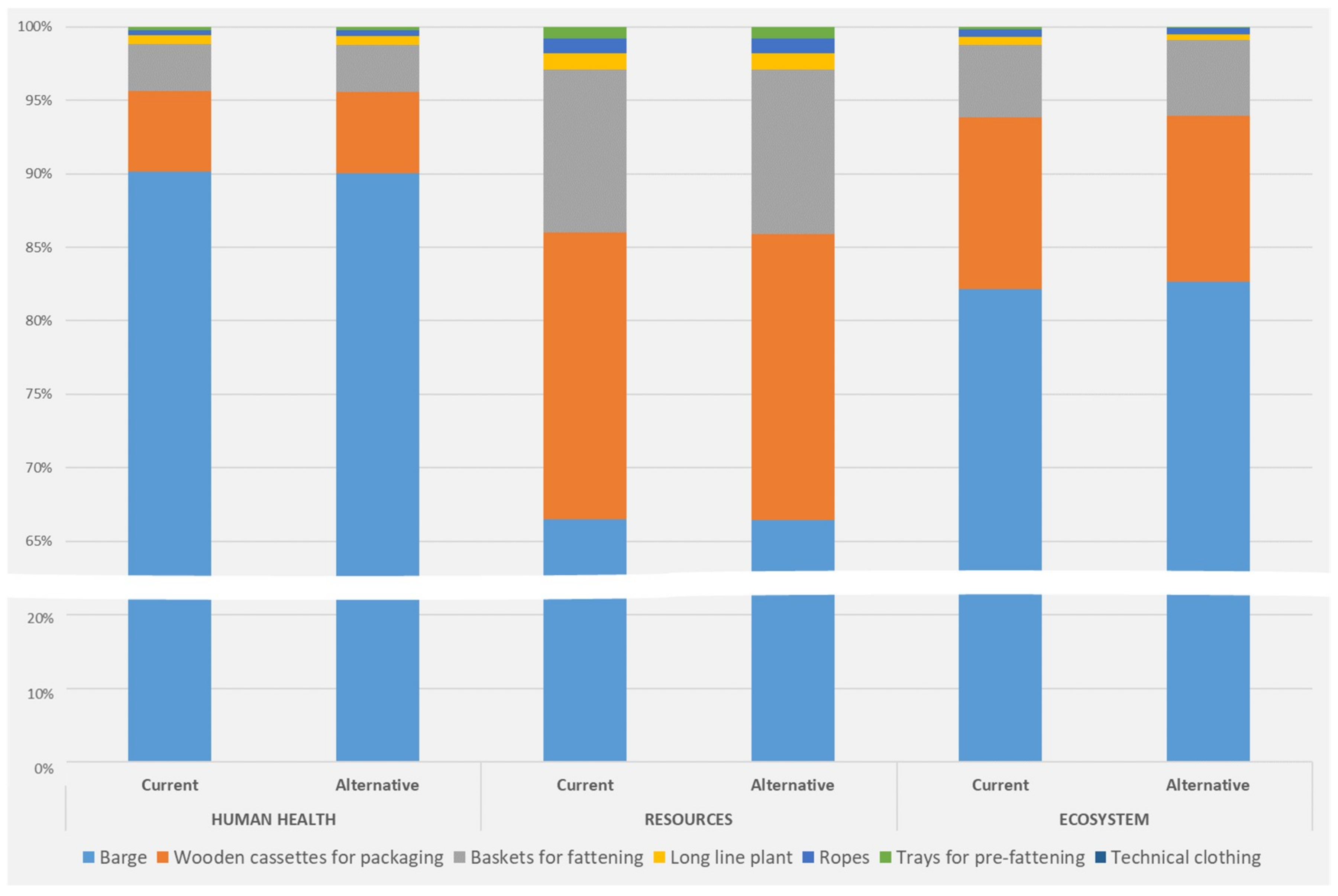
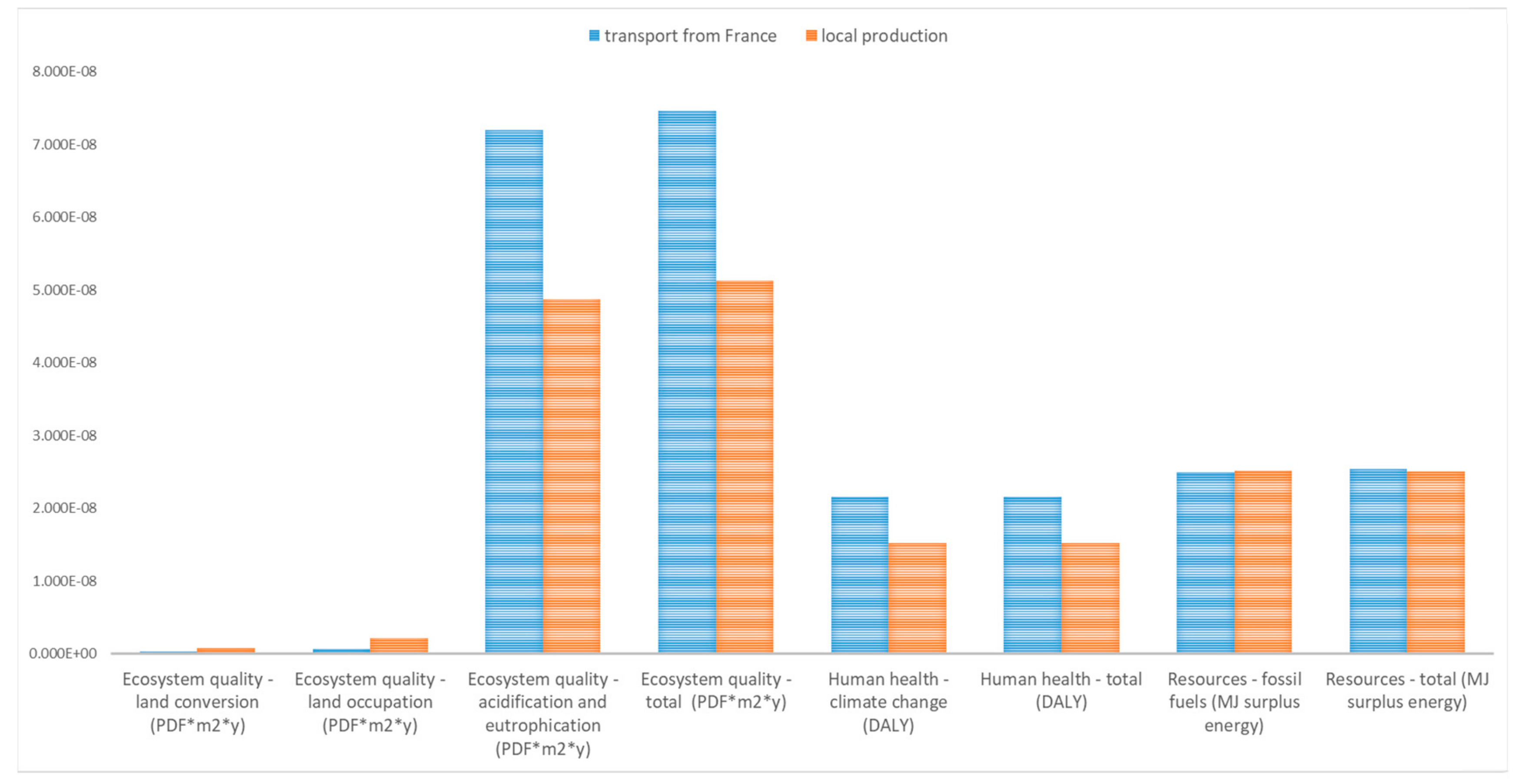
3. Results and Discussion

The LCIA results for both scenarios are presented in Table 3.
It is quite surprising that both scenarios showed almost identical environmental impacts in all categories, and, generally speaking, of very low value. The use of Ecoindicator® 99-H permits the evaluation of end-point impact categories in terms of damage to humans, resources, and ecosystems. In particular, the category human health refers to the theoretical concept that people should live their own genetically established lives, without interference by transmitted illnesses, disabilities, or premature deaths due to environmental causes. Otherwise, ecosystem quality is related to the idea that anthropogenic effects should not act on plant and animal survivor capacity or on their geographical distribution. Finally, the category resources permits an evaluation of the amount of nonrenewable resources the present population consumes, limiting their availability to future generations. An impact of 0.0101 disability-adjusted life years (DALYs) on human health means that oyster farming could contribute to the loss of about 5.5 days of life distributed over the overall population (not per person) [42]. As a reference, a default DALY value of 13 is usually adopted for the most severe effects on human health due to carcinogenic agents [43]. In our case, the effect on human health was so low it could be considered irrelevant, not due to the oyster culture itself but due to the indirect effect of climate change, i.e., due to the altered frequency and/or intensity of extreme weather events, local ecology of waterborne and foodborne infective agents, or the level of air pollution. Otherwise, the main contribution to ecosystem quality damage was represented by acidification and eutrophication due to ammonia, nitrogen oxides, and sulfur oxide emissions to the air from diesel fuel burning and the HDPE production process. The damage expressed in terms of the potentially disappeared fraction (PDF) can be interpreted as the potential fraction of species of vegetation that has a high probability of disappearing due to unfavorable conditions caused by the combined effects of acidification and eutrophication [44]. The output inventory results show that both scenarios of 1 kg of oyster production generate emissions to the air of 9.6 × 10⁻⁵ kg of ammonia, 3.0 × 10⁻⁴ of nitrogen oxides (NOx), and 5.2 × 10⁻⁴ kg of sulfur oxides (SOx). The value of 0.0312 PDF m2 year was derived from the specific contributions of 0.0016 PDF m2 year from ammonia, 0.0162 PDF m2 y from NOx, and 0.0054 PDF m2 year from SOx, corresponding to 11.24, 3.29, and 0.61 PDF m2 y per kg of emitted substance. These values are far below the reference for ecosystem damage reported in the “Eco-Indicator 99 Methodology” report [44], that is, 25.94, 9.52, and 1.73 PDF m2 year per kg, respectively. To have a comparative reference of the impact of oyster culture, we compared these results to other aquaculture productions, such as Finnish rainbow trout [45] and Spanish turbot [46], which were taken as a reference due to their large diffusion in the global market. The production of 1 kg of rainbow trout generates emissions into the air of 3.8 × 10⁻⁴ kg of ammonia, 5.8 × 10⁻³ of nitrogen oxides (NOx), and 1.8 × 10⁻³ kg of sulfur oxides (SOx), and the production of 1 kg of turbot burdens the air with 5.2 × 10⁻³ of nitrogen oxides (NOx) and 3.9 × 10⁻³ kg of sulfur oxides (SOx), which means an order of magnitude more in both cases with respect to oysters. It is obvious that a comparison of the edible parts of the two productions, namely oyster flesh and salmon fillets, would give even more of an extreme difference between oysters and salmon, underlining the intrinsic great value of oyster culture in terms of sustainability when compared to fish culture.
The Eco-Indicator 99 method does not consider the quantity of resources as such, but rather it provides indirect indicator. In our case, we can say that oyster farming requires abiotic resources, which determines the need for 0.76 MJ of surplus energy, which is consumed during supplying [47]. In particular, energy is needed for the extraction and production of fossil fuels and for the mining, grinding, and purification of minerals due to diesel fuel and plastic production, respectively.
Figure 4 shows the environmental impacts due to equipment and facilities as contribution trees for the two scenarios. In particular, it shows the relative contribution of equipment and facilities in terms of damage to human health, the damage to ecosystem quality and the damage to resources. It is clear that barges have the most impact, as confirmed by the results of carbon footprints reported in Reference [32], followed by the wooden cassettes for commercial packaging and the baskets for fattening. The contribution of the other equipment and facilities (ropes, trays for prefattening, and the long-line plant) are almost negligible (<1%). During one oyster production cycle, a barge is used about 110 times, covering an overall distance of about 1200 km and consuming about 800 l of diesel fuel per year. The baskets for fattening have a significant impact because they must be considered as nonrecyclable special waste due to the unremovable organic fouling that is deposited within the grids, even though they have an average lifespan of 8 years. In addition, in the case of the wooden cassettes, they cannot be reused, and in this analysis, they must be considered as one-way packaging. The use of technical clothing has a negligible impact on the overall supply chain. The blue and orange bars in Figure 4, which correspond to the current and alternative scenarios, respectively, are almost perfectly superimposed, because they differ only for the phases before prefattening and fattening (how to supply the seed). Apparently, any equipment and facilities used during oyster seed transport from France or during local oyster seed production have no significant effect on the overall oyster farming process impact.
Meanwhile, the impact derived from the use of equipment and facilities is very similar in the case of effects on human health, on ecosystem quality, and on category resources, which refers specifically to the use of resources, assuming a great impact of all nonrecyclable materials such as HDPE and wood compared to steel and other materials for barge construction.
Looking at the observations, it is not surprising that fattening is the most impactful step of farming (accounting for 74.5% on average of the three categories for the current scenario and 73.8% for the alternative scenario), followed by prefattening (13.1% for the current scenario and 13.0% for the alternative scenario), which is principally caused by the use of a barge in both cases. Oyster seed transport from France and local oyster seed production were confirmed to definitely account for a very low contribution of 0.13% and 0.10%, respectively. However, it is worthwhile pointing out that we did not compare the two different seed production processes, but rather the current production mode and the alternative local production (just the transport from France to Goro, not including production in the French farm in the current scenario, with effective complete local hatching and nursing in the alternative scenario). We neglected the contribution of step-seed production in France, because extending the boundaries to just the transportation was enough to support our conclusion that in-house seed production would be more convenient from an environmental point of view. Including the seed production in France would only have worsened and not changed the results. We compared two production systems rather than two processes with the same boundaries, with the aim of understanding which one should be chosen. As was the case in the “Joint research Centre (JRC) Recommendations” [48], we compared two systems that are not fully comparable, where comparability and equivalence are principally a matter of personal perception.
Focusing on the comparison between transportation and production (Figure 5), it is evident that local production had, overall, a lesser impact than did transportation from a place about 2000 km away. It can be imagined that including French oyster hatcheries in the overall impact of the current scenario would be higher than the impact herein calculated. Moreover, the general positive effect of setting up a completely local oyster farming supply chain has to be taken into account.
Except for categories related to sea conversion and occupation, for all impact categories, transport had a greater impact, surely due to diesel fuel consumption and the energy needed for refrigeration of the truck.
Impacts related to local production are caused by the use of plastic tubs and tanks, the supply of feed for spats, and the use of electric energy for pumps and building. Anyway, as mentioned above, all plastics are recyclable, and electric energy is supplied by a PV plant: de Alvarenga et al. [33] reported very low impacts for seed and oyster production, but they completely neglected inputs derived from the use of materials, feed, and cultivation plants, taking into account only water consumption, electricity, barges, and sea occupation.
The main evidence in this analysis was indeed the fact that a local supply chain permits the avoidance of a high burden of road transport, while assuring the complete traceability of the products. This, therefore, further strengthens the importance of a short supply chain in the production of primary goods, in particular in aquaculture.
Due to variations in the data collected as well as some estimates and assumptions used in this study, the Monte Carlo method was introduced to develop a statistical dispersion of the calculated outputs of the assessing model. The Monte Carlo analysis evaluates how the propagation of input variation is reflected in output values. The resulting output value corresponding to the impact category presents a mean value with a corresponding standard deviation (Table 4).
The results suggested that the fattening phase has the largest effect on ecosystem quality-related impacts, as suggested by the high coefficient of variation (CV), ecotoxicity in particular. The processes that have the highest weight on ecotoxicity during the fattening phase are related to reinforcing steel production and processing for barges (“reinforcing steel at plant, RER”: 56.23% and 56.16% for current and alternative scenarios, respectively). Nevertheless, even with the high level of uncertainty in the ecotoxicity, the results suggest that 95% of the time the ecotoxicity impact is <8.25 × 10⁻⁴ for the current scenario and 8.31 × 10⁻⁴ for the alternative one, which is two orders of magnitude lower compared to the ecotoxicity found by de Alvarenga et al. [33].
In order to compare the alternative scenario, that is, completely local oyster farming, to other aquaculture production, we had to recalculate the impact using a widespread method, the ReCiPe midpoint (H) v.1.12 method (Table 5). We report the results only for climate change, terrestrial acidification, marine and freshwater eutrophication, and water depletion, because they are the principal four impact categories provided in the literature about LCAs in aquaculture.
Unlike before, these are midpoint indicators that account for the “direct” impact of production outputs (i.e., emissions into the air and water) and not the potential damage to the overall environment. As can be seen in Table 6, oyster production is more sustainable, at least from an environmental point of view, than fish aquaculture, especially because oyster farming does not require a feeding supply during growth, which is the principal factor of vulnerability in fish farming. Otherwise, local oyster production seems to have environmental impacts similar to mussel farming in terms of kg CO2 eq (1.58) and kg SO2 eq (12.8 × 10⁻³), but it has lower eutrophication potential (10.1 × 10⁻³ for mussels versus 1.38 × 10⁻³ found for oysters) (as reported by Iribarren et al.) [45].
In addition to food production and beyond the discussion of carbon sequestration (estimated at 441 kg CO2/tons of oyster harvested) [32], oyster farming provides a series of other fundamental ecosystem services, such as the regulation of nitrogen levels in coastal areas [54]. Oysters, like other bivalves, can be cultivated in hypereutrophic coastal environments, which are affected by intense and harmful phytoplankton blooms. Evidence has been reported on bloom intensity and duration reduction where oysters are farmed, suggesting their positive effect as mitigating agents against coastal eutrophication [55].
Last but not least, oyster farming may also play an important role in benthic restoration and may represent a form of restoration of ecosystem services that was previously provided by overfished wild populations [56]. This is probably the most relevant positive effect of long-line oyster culturing. In fact, any productive activity brings area cover changes that usually turn out to be negative due to the leakage of naturality and wildness in favor of land/sea exploitation [57]. In the case of oyster culturing, although we were not able to account for it in the analysis, area cover occupation by the long-line turned into a provision of ecosystem services, since the sea area delimited by the long-line installation was interdicted to fishing activities, becoming a spawning and nursery ground for many species. At the same time, there were positive effects given by all the long-line structures, such as habitat and food niche diversification. These last terms deserve further research for proper inclusion in an LCA assessment.

4. Conclusions

An LCA of oyster farming was performed comparing the current scenario of production with seed purchased from France and an alternative scenario of a completely local supply chain from cradle-to-gate. In particular, our results demonstrate that the main hotspots are the fattening and prefattening stages of farming because of the use of barges and nonrecyclable plastic items. The LCA pointed out that, with respect to the current situation, local seed production provides several advantages, such as a lesser environmental impact and the possibility of improving the overall supply chain with complete local production. Furthermore, the results of this study strengthen the idea that an LCA could be effectively applied in the aquaculture sector to foster the development of environmentally sustainable production and improve the sustainable use of resources. Further improvements will be done in the near future, including different end-of-life scenarios for plastic items, i.e., the reuse, recycling, or disposal of materials. This work permitted us to identify the principal hotspot, which is undoubtedly the fattening phase. Some new productive solutions could be proposed and tested in order to reduce environmental impacts, e.g., barge use and fuel consumption optimization. Moreover, oyster production could become crucial for the economic development of some coastal areas: the real challenge will be to also include social and economic aspects and to realize an overall analysis of supply chain sustainability.

Supplementary Materials

The following are available online at https://www.mdpi.com/2079-9276/8/4/170/s1, Table S1: Total (inputs and outputs) background process requirements for the current scenario of oyster farming (amount cut-off of 0.1); Table S2: Total (inputs and outputs) background process requirements for the alternative scenario of oyster farming (amount cut-off of 0.1).

Author Contributions

Conceptualization, G.C. and E.T. (Edoardo Turolla); data and inventory, E.T. (Edoardo Turolla); methodology and formal analysis, E.T. (Elena Tamburini); writing—original draft preparation, E.T. (Elena Tamburini); writing—review and editing, all authors; supervision, E.A.F.

Funding

This research received no external funding.

Conflicts of Interest

The authors declare no conflicts of interest.

References

  1. Brooks, J.; Blandford, D. Chapter 2: Policies for Global Food Security. In Global Challenges for Future Food and Agricultural Policies, 1st ed.; Blandford, D., Hassapoyannes, K., Eds.; World Scientific Publishing Co Pte Ltd.: Singapore, 2019; Volume 1, pp. 5–38. [Google Scholar]
  2. Duarte, C.M.; Holmer, M.; Olsen, Y.; Soto, D.; Marbà, N.; Guiu, J.; Karakassis, I. Will the oceans help feed humanity? BioScience 2009, 59, 967–976. [Google Scholar] [CrossRef]
  3. Godfray, H.C.J. The debate over sustainable intensification. Food Secur. 2015, 7, 199–208. [Google Scholar] [CrossRef]
  4. Bringezu, S.; Ramaswami, A.; Schandl, H.; O’Brien, M.; Pelton, R.; Acquatella, J.; Ayuk, E.; Chiu, A.; Flanegin, R.; Fry, J.; et al. Assessing Global Resource Use: A Systems Approach to Resource Efficiency and Pollution Reduction; A Report of the International Resource Panel; United Nations Environment Programme: Nairobi, Kenya, 2017. [Google Scholar]
  5. Verdegem, M.C.J.; Bosma, R.H.; Verreth, J.A.J. Reducing water use for animal production through aquaculture. J. Water Resour. Dev. 2006, 22, 101–113. [Google Scholar] [CrossRef]
  6. Marra, J. When will we tame the oceans? Nature 2005, 436, 175–176. [Google Scholar] [CrossRef]
  7. FAO. The State of World Fisheries and Aquaculture 2018—Meeting the Sustainable Development Goals; Licence: CC BY-NC-SA 3.0 IGO; FAO: Rome, Italy, 2018; Available online: http://www.fao.org/3/i9540en/i9540en.pdf (accessed on 10 August 2019).
  8. Ding, Q.; Chen, X.; Chen, Y.; Tian, S. Estimation of catch losses resulting from overexploitation in the global marine fisheries. Acta Oceanol. Sin. 2017, 36, 37–44. [Google Scholar] [CrossRef]
  9. Hilborn, R.; Costello, C. The potential for blue growth in marine fish yield, profit and abundance of fish in the ocean. Mar. Policy 2018, 87, 350–355. [Google Scholar] [CrossRef]
  10. Cottrell, R.S.; Nash, K.L.; Halpern, B.S.; Remenyi, T.A.; Corney, S.P.; Fleming, A.; Blanchard, J.L. Food production shocks across land and sea. Nat. Sustain. 2019, 2, 130–137. [Google Scholar] [CrossRef]
  11. Morris, J.P.; Humphreys, M.P. Modelling seawater carbonate chemistry in shellfish aquaculture regions: Insights into CO2 release associated with shell formation and growth. Aquaculture 2019, 501, 338–344. [Google Scholar] [CrossRef]
  12. EEA. Aquaculture Production. 2019. Available online: https://www.eea.europa.eu/data-and-maps/indicators/ aquaculture-production-4/assessment (accessed on 23 July 2019).
  13. Bostock, J.; Lane, A.; Hough, C.; Yamamoto, K. An assessment of the economic contribution of EU aquaculture production and the influence of policies for its sustainable development. Aquac. Int. 2016, 24, 699–733. [Google Scholar] [CrossRef] [Green Version]
  14. Feinman, S.G.; Farah, Y.R.; Bauer, J.M.; Bowen, J.L. The influence of oyster farming on sediment bacterial communities. Estuaries Coasts 2018, 41, 800–814. [Google Scholar] [CrossRef]
  15. Khan, B.M.; Liu, Y. Marine Mollusks: Food with Benefits. CRFSFS 2019, 18, 548–564. [Google Scholar] [CrossRef]
  16. Lane, A.; Chatain, B.; Roque D’Orbacastel, E. Aquaculture in Occitanie, France. World Aquac. 2018, 49, 12–17. [Google Scholar]
  17. Marzano, A. Harvesting the Sea: The Exploitation of Marine Resources in the Roman Mediterranean; Oxford University Press: Oxford, UK, 2013; pp. 173–195. [Google Scholar]
  18. Oyster Trade, Product Trade, Exporters and Importers-OEC. Available online: https://oec.world/en/profile/hs92/030710/ (accessed on 24 July 2019).
  19. Orban, E.; Di Lena, G.; Masci, M.; Nevigato, T.; Casini, I.; Caproni, R.; Pellizzato, M. Growth, nutritional quality and safety of oysters (Crassostrea gigas) cultured in the lagoon of Venice (Italy). J. Sci. Food Agric. 2004, 84, 1929–1938. [Google Scholar] [CrossRef]
  20. Henriksson, P.J.; Guinée, J.B.; Kleijn, R.; de Snoo, G.R. Life cycle assessment of aquaculture systems—A review of methodologies. Int. J. Life Cycle Assess. 2012, 17, 304–313. [Google Scholar] [CrossRef]
  21. ISO 14040. Environmental Management—Life Cycle Assessment—Principles and Framework International Organization for Standardization, Geneva, Switzerland. 2006. Available online: https://www.iso.org/standard/37456.html (accessed on 24 July 2019).
  22. De Luca, A.I.; Iofrida, N.; Leskinen, P.; Stillitano, T.; Falcone, G.; Strano, A.; Gulisano, G. Life cycle tools combined with multi-criteria and participatory methods for agricultural sustainability: Insights from a systematic and critical review. Sci. Total Environ. 2017, 595, 352–370. [Google Scholar] [CrossRef]
  23. Tamburini, E.; Pedrini, P.; Marchetti, M.; Fano, E.; Castaldelli, G. Life cycle based evaluation of environmental and economic impacts of agricultural productions in the Mediterranean area. Sustainability 2015, 7, 2915–2935. [Google Scholar] [CrossRef]
  24. Pelletier, N.L.; Ayer, N.W.; Tyedmers, P.H.; Kruse, S.A.; Flysjo, A.; Robillard, G.; Sonesson, U. Impact categories for life cycle assessment research of seafood production systems: Review and prospectus. Int. J. Life Cycle Assess. 2007, 12, 414–421. [Google Scholar] [CrossRef]
  25. Besson, M.; Aubin, J.; Komen, H.; Poelman, M.; Quillet, E.; Vandeputte, M.; De Boer, I.J.M. Environmental impacts of genetic improvement of growth rate and feed conversion ratio in fish farming under rearing density and nitrogen output limitations. J. Clean Prod. 2016, 116, 100–109. [Google Scholar] [CrossRef] [Green Version]
  26. Vázquez-Rowe, I.; Iribarren, D.; Moreira, M.T.; Feijoo, G. Combined application of life cycle assessment and data envelopment analysis as a methodological approach for the assessment of fisheries. Int. J. Life Cycle Assess. 2010, 15, 272–283. [Google Scholar] [CrossRef]
  27. Ziegler, F.; Hornborg, S.; Green, B.S.; Eigaard, O.R.; Farmery, A.K.; Hammar, L.; Vázquez-Rowe, I. Expanding the concept of sustainable seafood using Life Cycle Assessment. Fish Fish. 2016, 17, 1073–1093. [Google Scholar] [CrossRef]
  28. García García, B.; Rosique Jiménez, C.; Aguado-Giménez, F.; García García, J. Life cycle assessment of gilthead seabream (Sparus aurata) production in offshore fish farms. Sustainability 2016, 8, 1228. [Google Scholar] [CrossRef]
  29. Iribarren, D.; Moreira, M.T.; Feijoo, G. Life Cycle Assessment of fresh and canned mussel processing and consumption in Galicia (NW Spain). Resour. Conserv. Recycl. 2010, 55, 106–117. [Google Scholar] [CrossRef]
  30. Lozano, S.; Iribarren, D.; Moreira, M.T.; Feijoo, G. Environmental impact efficiency in mussel cultivation. Resour. Conserv. Recycl. 2010, 54, 1269–1277. [Google Scholar] [CrossRef]
  31. Wijsman, J.W.M.; Troost, K.; Fang, J.; Roncarati, A. Global production of marine bivalves. Trends and challenges. In Goods and Services of Marine Bivalves; Smaal, A., Ferreira, J., Grant, J., Petersen, J., Strand, Ø., Eds.; Springer: Cham, Switzerland, 2019; pp. 7–26. [Google Scholar]
  32. Meyhoff Fry, J. Carbon Footprint of Scottish Suspended Mussels and Intertidal Oysters; Report Commissioned by SARF078 (Scottish Aquaculture Research Forum); Scottish Aquaculture Research Forum: Pitlochry, UK, 2012; ISBN 978-1-907266-44-7. [Google Scholar]
  33. De Alvarenga, R.A.F.; Galindro, B.M.; de Fátima Helpa, C.; Soares, S.R. The recycling of oyster shells: An environmental analysis using Life Cycle Assessment. J. Environ. Manag. 2012, 106, 102–109. [Google Scholar] [CrossRef]
  34. Nisticò, R. Aquatic-derived biomaterials for a sustainable future: A European opportunity. Resources 2017, 6, 65. [Google Scholar] [CrossRef]
  35. Turolla, E.; Savorelli, F.; Palazzi, D.; Gelli, F. Impiego di tecniche di induzione all’emissione dei gameti in Crassostrea gigas per l’esecuzione di test di embriotossicita. Boll. Malacol. 2008, 43, 73. (In Italian) [Google Scholar]
  36. Walne, P.R. The culture of marine bivalve larvae. Physiol. Mollusca 1946, 1, 197–210. [Google Scholar]
  37. Ecoinvent Database®. Available online: https://www.ecoinvent.org/database/database.html (accessed on 9 October 2019).
  38. Blanc, I.; Friot, D.; Margni, M.; Jolliet, O. Towards a new index for environmental sustainability based on a DALY weighting approach. Sustain. Dev. 2008, 16, 251–260. [Google Scholar] [CrossRef] [Green Version]
  39. ReCiPe®. Available online: https://www.pre-sustainability.com/recipe (accessed on 19 September 2019).
  40. Reap, J.; Roman, F.; Duncan, S.; Bras, B. A survey of unresolved problems in life cycle assessment. Int. J. Life Cycle Asses. 2008, 13, 374–388. [Google Scholar] [CrossRef]
  41. Avadí, A.; Fréon, P. Life cycle assessment of fisheries: A review for fisheries scientists and managers. Fish. Res. 2013, 143, 21–38. [Google Scholar] [CrossRef]
  42. Murray, C.J.; Lopez, A.D. Evidence-based health policy—lessons from the Global Burden of Disease Study. Science 1996, 274, 740–743. [Google Scholar] [CrossRef] [PubMed]
  43. Klepper, O.; Bakker, J.; Traas, T.P.; van de Meent, D. Mapping the potentially affected fraction (PAF) of species as a basis for comparison of ecotoxicological risks between substances and regions. J. Hazard Mater. 1998, 61, 337–344. [Google Scholar] [CrossRef]
  44. Goedkoop, M.; Spriensma, R. The Eco-Indicator 99 a Damage Oriented Method for Life Cycle Impact Assessment; PRé Consultants: Amersfoort, The Netherlands, 2001. [Google Scholar]
  45. Gronroos, J.; Seppala, J.; Silvenius, F.; Makinen, T. Life cycle assessment of Finnish cultivated rainbow trout. Boreal Environ. Res 2006, 11, 401–414. [Google Scholar]
  46. Iribarren, D.; Moreira, M.T.; Feijoo, G. Life Cycle Assessment of Aquaculture Feed and Application to the Turbot Sector. Int. J. Environ. Res. 2012, 6, 837–848. [Google Scholar]
  47. Iribarren, D.; Moreira, M.T.; Feijoo, G. Revisiting the life cycle assessment of mussels from a sectorial perspective. J. Clean. Prod. 2010, 18, 101–111. [Google Scholar] [CrossRef]
  48. European Commission—Joint Research Centre—Institute for Environment and Sustainability. International Reference Life Cycle Data System (ILCD) Handbook—General Guide for Life Cycle Assessment—Detailed Guidance, 1st ed.; EUR 24708 EN; Publications Office of the European Union: Luxembourg, Luxembourg, 2010. [Google Scholar]
  49. Jerbi, M.A.; Aubin, J.; Garnaoui, K.; Achour, L.; Kacem, A. Life cycle assessment (LCA) of two rearing techniques of sea bass (Dicentrarchus labrax). Aquac. Eng. 2012, 46, 1–9. [Google Scholar] [CrossRef]
  50. Samuel-Fitwi, B.; Nagel, F.; Meyer, S.; Schroeder, J.P.; Schulz, C. Comparative life cycle assessment (LCA) of raising rainbow trout (Oncorhynchus mykiss) in different production systems. Aquac. Eng. 2013, 54, 85–92. [Google Scholar] [CrossRef]
  51. Abdou, K.; Aubin, J.; Romdhane, M.S.; Le Loc’h, F.; Lasram, F.B.R. Environmental assessment of seabass (Dicentrarchus labrax) and seabream (Sparus aurata) farming from a life cycle perspective: A case study of a Tunisian aquaculture farm. Aquaculture 2017, 471, 204–212. [Google Scholar] [CrossRef]
  52. Aubin, J.; Papatryphon, E.; Van der Werf, H.M.G.; Petit, J.; Morvan, Y.M. Characterisation of the environmental impact of a turbot (Scophthalmus maximus) re-circulating production system using Life Cycle Assessment. Aquaculture 2016, 261, 1259–1268. [Google Scholar] [CrossRef]
  53. Pelletier, N.; Tyedmers, P.; Sonesson, U.; Scholz, A.; Ziegler, F.; Flysjo, A.; Silverman, H. Not All Salmon are Created Equal: Life Cycle Assessment (LCA) of Global Salmon Farming Systems. Environ. Sci. Technol. 2009, 43, 8730–8736. [Google Scholar] [CrossRef]
  54. Filgueira, R.; Byron, C.J.; Comeau, L.A.; Costa-Pierce, B.; Cranford, P.J.; Ferreira, J.G.; McKindsey, C.W. An integrated ecosystem approach for assessing the potential role of cultivated bivalve shells as part of the carbon trading system. Mar. Ecol. Prog. Ser. 2015, 518, 281–287. [Google Scholar] [CrossRef] [Green Version]
  55. Rice, M.A. Environmental impacts of shellfish aqua-culture: Filter feeding to control eutrophication. In Proceedings of the Workshop on Aquaculture and the Marine Environment: A Meeting for Stakeholders in the Northeast, University of Massachusetts, Boston, MA, USA, 11–13 January 2001; pp. 1–11. [Google Scholar]
  56. Mallet, A.L.; Carver, C.E.; Landry, T. Impact of suspended and off-bottom Eastern oyster culture on the benthic environment in eastern Canada. Aquaculture 2006, 255, 362–373. [Google Scholar] [CrossRef]
  57. Huntington, T.C.H.; Roberts, N.; Cousins, V.; Pitta, N.; Marchesi, A.; Sanmamed, T.; Hunter-Rowe, T.F.; Fernandes, P.; Tett, J.; Cue, M.; et al. Some Aspects of the Environmental Impact of Aquaculture in Sensitive Areas; Report to the DG Fish and Maritime Affairs of the European Commission; Poseidon Aquatic Resource Management Ltd.: Hampshire, UK, 2006. [Google Scholar]
Figure 1. Location of the oyster culture leases on the northeastern coast of Italy (a) in Sacca di Goro (b). The positions of the two sites (for seed-oyster hatching (SH) and for off-shore oyster growing (LL)) are indicated.
Resources 08 00170 g001
Figure 2. Simplified scheme of the main principles of a submerged long-line plant for oyster end-fattening: 1, head-buoys; 2, buoys; 3, anchoring blocks; 4, floating system; 5, span; 6, mooring; 7, baskets for oyster fattening; 8, trays for oyster prefattening.
Resources 08 00170 g002
Figure 3. System boundaries used in the life cycle assessment (LCA) of oyster production in Goro under the two proposed scenarios: (a) the current scenario (purchasing seed from France); and (b) the alternative scenario (local nursing and hatching). The boxes represent processes (solid box = foreground process; dashed box = background process; dash–dot box = raw material production process/electricity production), and gray circles represent products. Solid arrows depict mass flows, and dashed lines indicate energy flows.
Resources 08 00170 g003aResources 08 00170 g003b
Figure 4. Results of LCIA method (Ecoindicator), expressed in terms of contribution trees for the three damage categories, human health, and ecosystem quality (comparing the current and alternative scenarios).
Resources 08 00170 g004
Figure 5. Comparison between environmental impacts of transport from France and local seed production (LCIA: Ecoindicator®) (impact categories with values <10−7 were neglected as a single column but were included in the total values).
Resources 08 00170 g005
Table 1. Inventory of main inputs for the two different scenarios: seed from France and local seed production. The value 0 tons km means that the contribution of transport is negligible, since the supplier is located in Goro. The transport of raw materials to suppliers was not included in the analysis. All inputs are referred to in terms of 12 fresh oysters for production (1 kg of oysters).
InputsSeed from FranceLocal Seed
Resources
Sea use (m2 year−1)-120,000
Seawater (m3)-160
Freshwater (m3)-16
Materials and fuel
High-density polyethylene (HDPE) (kg)-181.3
Polypropylene (PP) (kg)-16
Polyvinyl chloride (PVC) (kg)-1.24
Rubber (kg)-0.95
Glass fiber (kg)-2.7
Nylon (kg)-63
Concrete (kg)-144
Steel (kg)-0.6
Diesel for boat (l)-800
Wood (kg)-160
Chemicals
Salt solution for feed (g)-40
Vitamins for feed (g)-6
CO2 (L)-90
Energy
Electrical energy (kWh)34.2 *1400
Vehicles
Boat (no. of items)-0.033
Transport from suppliers to Goro
Seed from L’Epine, France to Goro (tons km)1600
Tanks for seed production (tons km)-40.3
Prefattening trays (tons km)-2.23
Ropes (tons km)-0
PVC and rubber clothing (tons km) -0
Fattening baskets (tons km)-24.8
Cassettes for selection (tons km)-0.82
Wood cassettes for packaging (tons km)-0
Emissions to air
Carbon dioxide (kg)0.5060.001
Nitrous oxide (kg)0.00145.29 × 10−6
Sulfur dioxide (kg)0.00080.0006
Methane (kg)3.26 × 10−63.48 × 10−6
Nonmethane volatile organic carbon (NMVOC) (kg)0.00250.0025
Particulates <2.5 μ (kg)0.000230.00023
Particulates >10 μ (kg)4.78 × 10−54.51 × 10−5
Particulates >2.5 μ and <10 μ (kg)6.86 × 10−56.63 × 10−5
Emissions to water
Adsorbable organic halogen as Cl (AOX) (kg) 1.84 × 10⁻⁹
Biochemical oxygen demand (BOD) (kg) 0.00062
Heat, waste (MJ) 6.79 × 10⁻⁵
Nitrate (kg) 2.21 × 10⁻⁶
* The contribution of energy to transport is related to the need for refrigeration.
Table 2. Impact categories considered in this study.
Impact CategoryUnit
Human health: totalDALY *
Human health: climate changeDALY
Human health: carcinogenicDALY
Human health: respiratory effects caused by chemical substancesDALY
Human health: ozone layer depletionDALY
Ecosystem quality: totalPDF m2 year **
Ecosystem quality: sea conversionPDF m2 year
Ecosystem quality: sea occupationPDF m2 year
Ecosystem quality: acidification and eutrophicationPDF m2 year
Ecosystem quality: ecotoxicityPDF m2 year
Resources: totalMJ surplus energy ***
Resources: fossil fuelsMJ surplus energy
Resources: mineralsMJ surplus energy
Notes: * DALY = disability-adjusted life year, a measure of overall disease burden, expressed as the number of years lost due to ill health, disability, or early death. ** PDF m2 year = The potentially disappeared fraction represents the fraction of species that disappear from 1 m2 of earth surface over one year. *** MJ surplus energy = a measure of the amount of energy extracted or needed to extract a resource.
Table 3. Impact categories considered in this study.
Impact CategoryCurrent
(Seeds from France)
Alternative
(Seeds In Situ)
Unit
Human health: total0.01040.0104DALY
Human health: climate change0.01010.0101DALY
Human health: carcinogenic7.26 × 10−67.26 × 10⁻⁶DALY
Human health: respiratory effects caused by chemical substances2.31 × 10−62.31 × 10⁻⁶DALY
Human health: ozone layer depletion1.26 × 10−101.26 × 10⁻¹⁰DALY
Ecosystem quality: total0.02980.0298PDF m2 year
Ecosystem quality: sea conversion0.00110.0011PDF m2 year
Ecosystem quality: sea occupation0.00230.0023PDF m2 year
Ecosystem quality: acidification and eutrophication0.03160.0315PDF m2 year
Ecosystem quality: ecotoxicity0.00020.0002PDF m2 year
Resources: total0.75440.7543MJ surplus energy
Resources: fossil fuels0.74670.7466MJ surplus energy
Resources: minerals0.00770.0077MJ surplus energy
Table 4. Results of a Monte Carlo simulation for impact categories calculated for the current and alternative scenarios. CV, coefficient of variation
Impact CategoryMeanSDCV%MinMaxMedian5% 95%
Current Scenario
Human health: total1.11 × 10−21.64 × 10−313%8.40 × 10−31.64 × 10−21.11 × 10−28.64 × 10−31.38 × 10⁻²
Human health: climate change1.11 × 10−21.64 × 10−313%8.39 × 10−31.63 × 10−21.10 × 10−28.63 × 10−31.38 × 10⁻²
Human health: carcinogenics9.52 × 10−64.14 × 10−650%2.40 × 10−62.63 × 10−59.00 × 10−64.78 × 10−61.69 × 10⁻⁵
Human health: respiratory effects 3.40 × 10−66.14 × 10−725%2.18 × 10−65.23 × 10−63.33 × 10−62.54 × 10−64.65 × 10⁻⁶
Human health: ozone layer depletion1.78 × 10−16.00 × 10−1129%8.32 × 10−114.64 × 10−101.71 × 10−109.87 × 10−112.86 × 10⁻¹⁰
Ecosystems: total4.38 × 10−21.03 × 10−236%2.79 × 10−29.14 × 10−24.21 × 10−23.15 × 10−26.31 × 10⁻²
Ecosystem quality: sea conversion1.43 × 10−36.75 × 10−442%6.61 × 10−45.03 × 10−31.26 × 10−37.69 × 10−43.22 × 10⁻³
Ecosystem quality: sea occupation2.61 × 10−37.99 × 10−427%1.24 × 10−35.25 × 10−32.48 × 10−31.66 × 10−34.19 × 10⁻³
Ecosystem quality: acidification and eutrophication3.98 × 10−21.01 × 10−239%2.53 × 10−28.73 × 10−23.74 × 10−22.77 × 10−26.02 × 10⁻²
Ecosystem quality: ecotoxicity4.22 × 10−42.91 × 10−464%1.33 × 10−42.77 × 10−33.58 × 10−42.20 × 10−48.25 × 10⁻⁴
Resources: total8.23 × 10−11.31 × 10−114%5.57 × 10−11.17 7.99 × 10−16.69 × 10−11.04
Resources: fossil fuels8.15 × 10−11.30 × 10−114%5.50 × 10−11.16 7.92 × 10−16.62 × 10−11.04
Resources: minerals8.03 × 10−39.29 × 10−411%6.23 × 10−31.09 × 10−27.93 × 10−36.62 × 10−39.63 × 10⁻³
Alternative Scenario
Human health: total1.11 × 10−21.41 × 10−315%7.69 × 10−31.49 × 10−21.10 × 10−29.14 × 10−31.36 × 10⁻²
Human health: climate change1.11 × 10−21.41 × 10−315%7.68 × 10−31.49 × 10−21.10 × 10−29.13 × 10−31.36 × 10⁻²
Human health: carcinogenics1.01 × 10−55.00 × 10−643%3.06 × 10−63.62 × 10−58.80 × 10−64.60 × 10−61.96 × 10⁻⁵
Human health: respiratory effects 3.50 × 10−68.60 × 10−718%2.20 × 10−69.20 × 10−63.34 × 10−62.58 × 10−65.00 × 10⁻⁶
Human health: ozone layer depletion1.73 × 10−105.01 × 10−1134%7.64 × 10−114.43 × 10−101.67 × 10−101.14 × 10−102.64 × 10⁻¹⁰
Ecosystem quality: total4.59 × 10−21.67 × 10−223%2.87 × 10−21.51 × 10−14.23 × 10−23.14 × 10−26.82 × 10⁻²
Ecosystem quality: sea conversion1.44 × 10−36.09 × 10−447%6.88 × 10−44.98 × 10−31.30 × 10−38.07 × 10−42.75 × 10⁻³
Ecosystem quality: sea occupation2.51 × 10−36.87 × 10−431%1.19 × 10−34.68 × 10−32.37 × 10−31.69 × 10−34.02 × 10⁻³
Ecosystem quality: acidification and eutrophication4.20 × 10−21.65 × 10−225%2.62 × 10−21.48 × 10−13.78 × 10−22.80 × 10−26.43 × 10⁻²
Ecosystem quality: ecotoxicity4.19 × 10−42.68 × 10−469%1.49 × 10−41.94 × 10−3354 × 10−42.04 × 10−48.31 × 10−4
Resources: total836 × 10−11.19 × 10−116%5.71 × 10−11.168.27 × 10−16.70 × 10−11.06
Resources: fossil fuels8.28 × 10−11.19 × 10−116%5.62 × 10−11.158.20 × 10−16.63 × 10−11.05
Resources: minerals8.26 × 10−39.27 × 10−412%6.33 × 10−31.04 × 10−28.26 × 10−36.87 × 10−31.01 × 10⁻²
Table 5. Environmental impacts per 1 kg of fresh oysters based on the ReCiPe midpoint (H) v.1.12 method.
Impact CategoryAlternative
Scenario
(Seed in situ)
Unit
Climate change1.85Kg CO2 eq
Terrestrial acidification9.29 × 10−3Kg SO2 eq
Marine and freshwater eutrophication1.38 × 10−3Kg PO4 eq
Water depletion31.76l
Table 6. Environmental impacts per 1 kg of fresh fish products.
TitleClimate Change
(kg CO2 eq)
Eutrophication
(kg PO4 eq)
Acidification
(kg SO2 eq)
Water Dependence (m3)Ref.
Sea bass11.00–17.00180–240 × 10−350–80 × 10−3190–396Jerdi et al. [49]
Rainbow trout2.24–13.624.04–60.36 × 10−310.43–40.72 × 10⁻³-Samuel-Fitwi et al. [50]
Sea bream3.6798.8621.61-Adbou et al. [51]
Sea bass3.1891.0318.85-
Turbot6.0280 × 10−350 × 10−3-Aubin et al. [52]
Salmon2.1649 × 10−320.4 × 10⁻³-Pellettier et al. [53]

