Urban Water Demand Forecasting: A Comparative Evaluation of Conventional and Soft Computing Techniques

Abstract

Previous studies have shown that soft computing models are excellent predictive models for demand management problems. However, their applications in solving water demand forecasting problems have been scantily reported. In this study, feedforward artificial neural networks (ANNs) and a support vector machine (SVM) were used to forecast water consumption. Two ANN models were trained using different algorithms: differential evolution (DE) and conjugate gradient (CG). The performance of these soft computing models was investigated with real-world data sets from the City of Ekurhuleni, South Africa, and compared with conventionally used exponential smoothing (ES) and multiple linear regression (MLR). The results obtained showed that the ANN model that was trained with DE performed better than the CG-trained ANN and other predictive models (SVM, ES and MLR). This observation further demonstrates the robustness of evolutionary computation techniques amongst soft computing techniques.

1. Introduction

The United Nations’ (UN) Vision 2050 aims to ensure that enough and safe water is made available to meet every person’s basic needs, with healthy lifestyles and behaviors easily upheld through reliable and affordable water supply and sanitation services [1]. To this end, in its World Water Development Report (2015), it identified the validating and tailoring of data for water management decision-making systems as one of the outstanding challenges to be met in knowledge generation and policy formulation. To solve this problem, water forecasting models are required to make water management policies more efficient [2]. However, for water demand forecasting to be effective in achieving this aim, there is a need to improve the current water demand models. The conventional “fixture-unit” approach (typically based on multivariate regression and time-series analysis), often employed by water utilities and municipalities, has been criticized for (i) having its working principles based on the assumption of collinearity [3,4], and (ii) having several inherent uncertainties resulting in overestimations of actual water demand at as much as 100% [5].

Water distribution systems are designed to satisfy consumers’ requirements both in the short- and long-terms. Long-term forecasts are imperative for planning and infrastructure design, for instance, in providing new water supplies and upgrading the capacity of existing water treatment plants, while short-term forecasts provide guidance in operating and managing water resources and associated infrastructure e.g., day-to-day operation of treatment plants and reservoirs to meet daily demands [2]. Accurate water demand forecasts are, therefore, required for short- and long-term infrastructure planning, operation and coordination.

Most of the existing water demand models lack the capacity to account for the ever-increasing trends in urbanization, rapid population, socio-economic growth and climate change; therefore, new models for water demand forecasting are required to handle these variables [6]. The models should be able to account for the dynamic and complex interactions among demographic, environmental, technological and socioeconomic characteristics of a water system. This is key to building a secure water future at both local and global scales, thereby fostering the realization of the UN objectives.

To develop robust models for water management, researchers are now using soft computing techniques to address water resource problems. This growing interest has been attributed to the abilities of soft computing techniques to provide a high degree of accuracy, tractability, robustness, and cost-effective solutions to complex, ambiguous, dynamic and nonlinear real-world problems [7]. Currently, there are reports on the application of artificial neural networks (ANNs) [8], support vector machines (SVMs) [9], adaptive neuro-fuzzy inferences systems (ANFISs) [10], systems dynamics [11] and evolutionary computation (EC)-based metaheuristics [12] as methods for solving water resource problems. The results from these techniques’ applications have helped to increase confidence in the modeling approach for water resource planning problems [13,14,15,16,17,18,19]. Because of their success, these techniques are now being envisaged to replace or complement the conventional and/or traditional modeling techniques [20].

Research suggests that, despite the recent advances in the application of soft computing techniques, several areas are yet to be maximized in water demand forecasting [7,21]. Ghalehkhondabi, Ardjmand, Young and Weckman [7] present a comprehensive review of soft computing techniques’ application in water demand forecasting. They suggest that investigation into the potential of new artificial intelligence (AI) and metaheuristic techniques (deep neural nets and EC techniques) should be carried out in future studies to improve the planning, operation and management of water resources. According to the authors, AI and metaheuristics can be used to optimize model architectures. They also suggest a shift from short-term to medium- and long-term forecasting. Oyebode, Babatunde, Monyei and Babatunde [21] report that evolutionary computation (EC) techniques, such as differential evolution (DE), have not been adequately used to model water demand. Their review suggests that the adoption of EC techniques in water demand forecasting is yet to be embraced in developing countries. Furthermore, Shabani, Yousefi, Adamowski and Naser [5] recommend the inclusion of weather and socio-economic variables in long-term water demand forecasting models. Considering the importance of water demand forecasting, and the need to improve the accuracy of forecasts, more research is required to fully harness soft computing technique potential. Given the successes recorded in the use of AI and EC techniques in short-term water demand forecasting [7,21], it is envisaged that these techniques would be useful in developing long-term water demand forecasts.

To address the above-mentioned knowledge gaps, this study investigated the potential of two soft computing techniques (ANN and SVM) as predictive models for municipal water demand forecasting. It sought to investigate the impacts of training algorithms on the learning ability of feedforward ANNs. To this end, two ANN models were developed using different training algorithms—differential evolution (DE) and conjugate gradient (CG) algorithms. These models’ performance was compared to a multiple linear regression (MLR) and exponential smoothing (ES).

2. Materials and Methods

This study entailed the use of five different techniques for monthly water demand forecasting. Two of the models were based on the working principles of ANN, while the other three models were SVM, MLR and ES. The remaining sub-sections present brief description of these methods.

2.1. Multiple Linear Regression

Linear regression (LR) is a popular statistical technique that has been widely used to forecast water demand [22,23]. When this model is used to predict two or more dependent parameters (regressors), it is called a multiple linear regression (MLR) model (Equation (1)).

$$Y={\beta }_o+{\beta }_1{X}_1+{\beta }_2{X}_2+\dots +{\beta }_k{X}_k+E$$

(1)

where ${\beta }_o, {\beta }_1, {\beta }_2, \dots , {\beta }_k$ are the regression coefficients, $E \mathrm{and} Y$ are error and dependent parameters, respectively, and $X_1, X_2, \dots , X_x$ are independent variables. The performance of an MLR model can be estimated with its error value. This is the difference between observed and predicted values. The coefficient correlation $\left(r\right)$ and coefficient of determination $\left(R^2\right)$ are performance measures which are sometimes used to analyze MLR models’ performance. Technically, a regression model uses a least-squares method to minimize the sum of squares of the difference between the observed and predicted parameters.

2.2. Exponential Smoothing

ES, which is a member of the moving average forecasting methods, uses the weighted averages of past observations to forecast dependent parameters. Old data sets’ weights decay exponentially [24], while new data sets are given relatively bigger weights. This model forecasts dependent parameters based on the weighted sum of observed values (Equation (2)). The fundamental idea of this model is that the trend of the time series is stable or regular, and the time series trend can be reasonably postponed, and thus, the latest historical trend will persist into the future [25]. ES forecast accuracy depends on the value of a smoothing (α) or a damping (1 − α) factor. Although, no formal procedure exists for choosing an α value; researchers often adopt a trial-and-error method when selecting an α value [24].

$$F_{t+1}=F_t+\alpha \left(A_t-F_t\right)$$

(2)

where $A_t$ is the actual value at time $t,$ $F_t$ is the forecast value at time $t$, $F_{t+1}$ is the forecast value at time $t+1,$ and $\alpha$ is a smoothing factor, $0\le \alpha \le 1$.

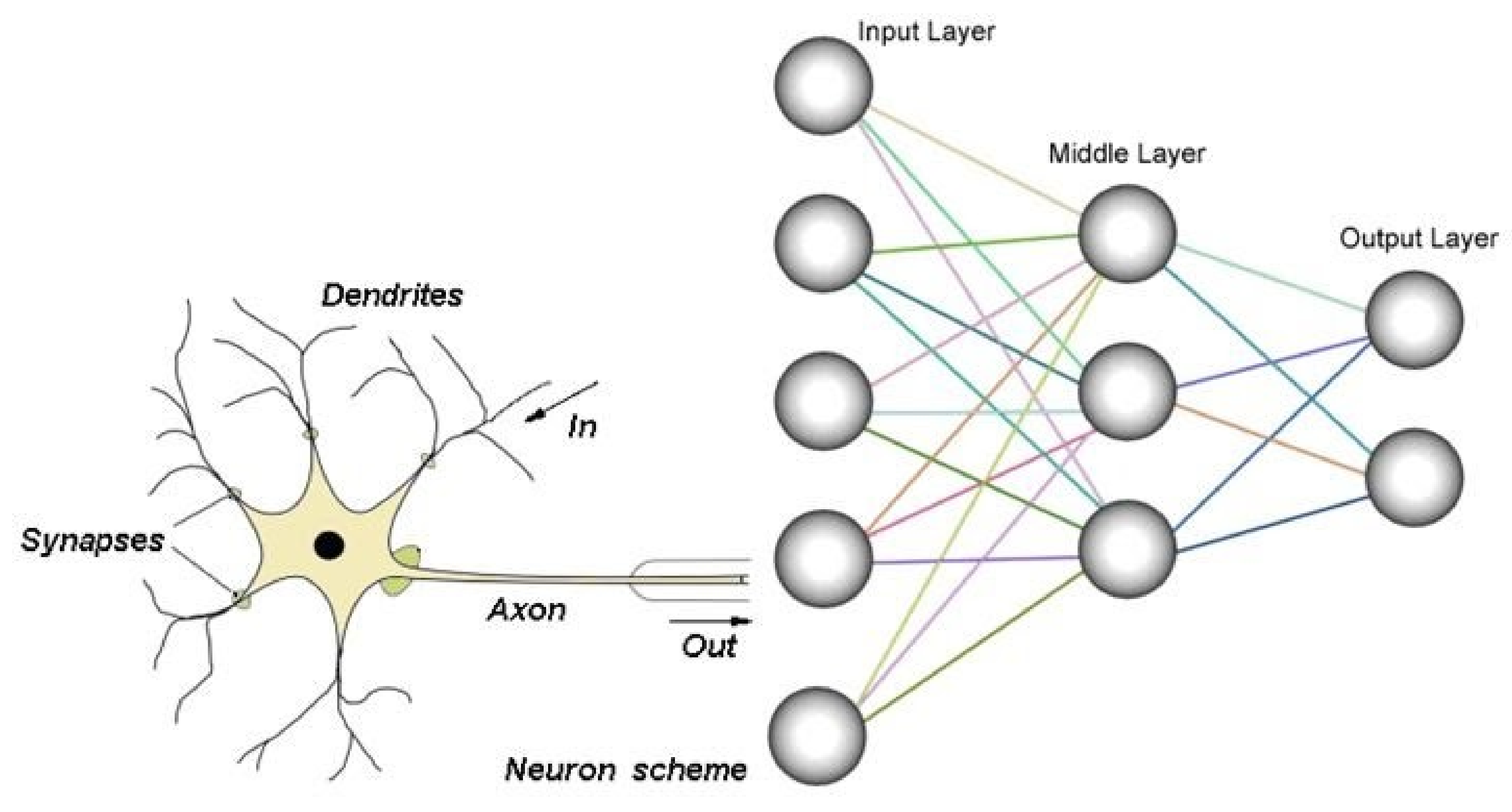
2.3. Artificial Neural Network

An ANN is a soft computing technique inspired by the configuration and working principles of the human nervous system [26]. Its structure encompasses a pool of artificial neurons or perceptrons, typically assembled in three layers which collect, interpret and exchange information over a framework of weighted connections, see Figure 1 [20]. Through a process of training, ANN forecast output parameters by combining the input data set with connection weights. These weights are adjusted during the training of an ANN model using a training algorithm and an activation function. An ANN model, therefore, undergoes a learning process by adjusting its connection weights iteratively using its error value(s) and input parameters [27]. Given a sigmoidal activation function, the relationship between inputs and output(s) is expressed as:

$$P=1/\left(1+e^s\right),$$

(3)

$$s=\left(a_1{w}_1+a_2{w}_2+\dots \right)+B$$

(4)

where $P$ is the output of each node, $a_i$ is the input value, $w_i$ is the weight, and $B$ denotes bias.

The key objective of ANN training is to reduce the overall error $E$ between the predicted and actual observations. The overall error of an ANN model, $E,$ is mathematically expressed as [28]:

$$E=\frac{1}{m}{{\displaystyle \sum }}^{\text{}}{E}_m,$$

(5)

where $m$ is the total number of training patterns and $E_m$ is expressed as Equation (6)

$$E_m=\frac{1}{2}{{\displaystyle \sum }}^{\text{}}{\left(O_n-P_n\right)}^2,$$

(6)

where, $O_n$ and $P_n$ are actual and predicted values for $n$th output processor, respectively.

Details on ANN model configuration and implementation are available in the literature [20,27]. On the other hand, information on the selected training algorithms—DE and conjugate gradient (CG)—are available in References [29,30].

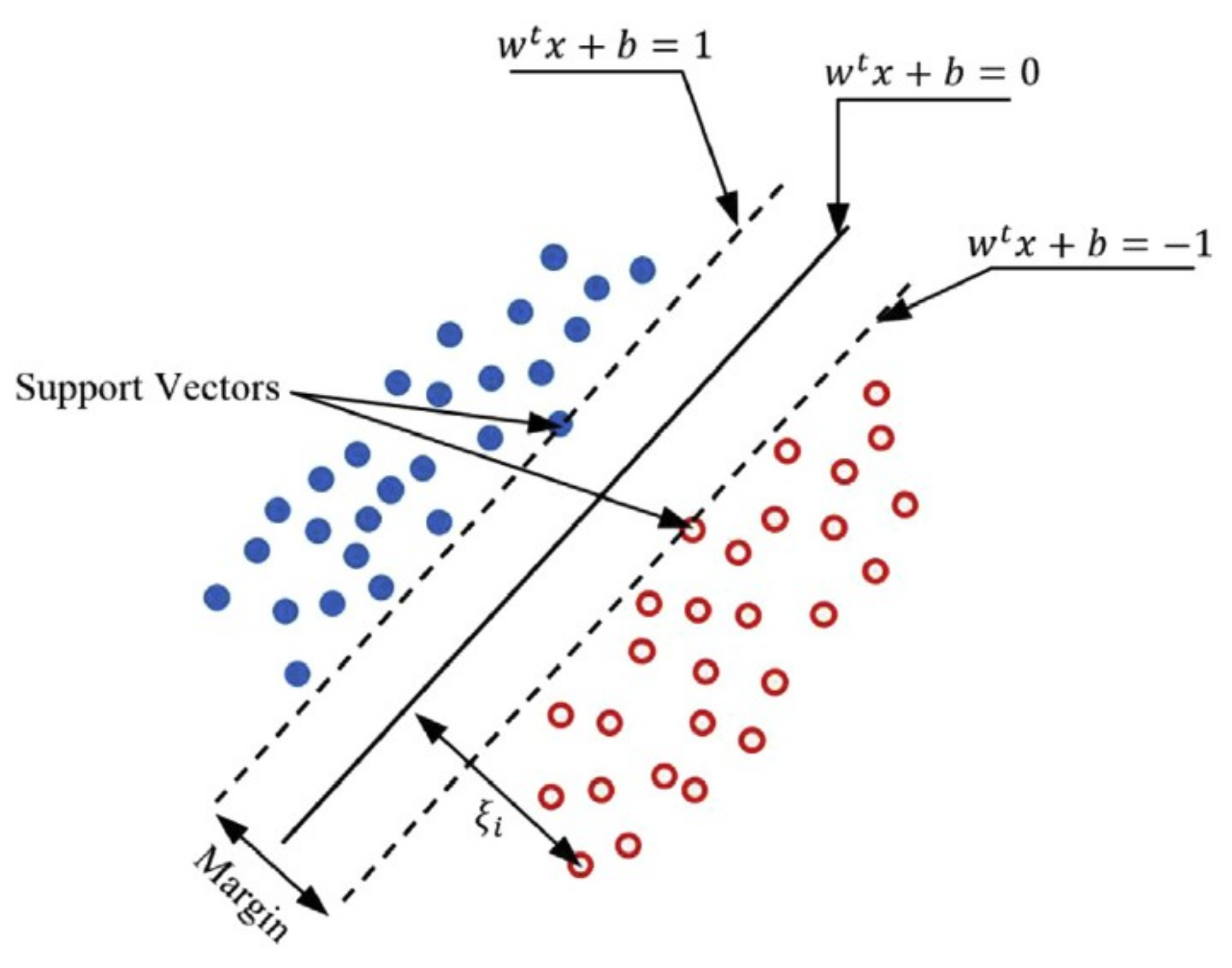
2.4. Support Vector Machine

SVM is a soft computing method that originates from statistical learning theory [32]. It uses a supervised learning approach to solve regression, density estimation and classification problems. An SVM is initialized by defining a practical limit or boundary on the generalization error using a structural risk minimization (SRM) principle [33]. It thereafter advances to search for the optimal structure of a model, using predefined model training parameters to guarantee an exclusive global minimum of the error surface. SVM, therefore, uses a nonlinear transformation to map input space into higher feature dimensional space. This approach enables it to have a good performance in terms of generalization. The mapping function which is implemented using a specified kernel may either be a linear, polynomial, sigmoidal, radial basis or hybrid function.

This model working principle is like that of an ANN model; both models can be represented as two-layered networks wherein the weights are nonlinear and linear in the first and output layers, respectively [34]. However, unlike ANN wherein an adaptive learning approach is adopted in optimizing its parameters, SVM selects its parameters for the first layer as training input vectors. One of the advantages of SVM is that it works with smaller amount of training samples and variables [35].

In a regression-based SVM, the training data sets is defined as $\left[x_i, y_i\right],$ where $x_i\in R^n$ is the input vector, $n$ is the dimension of input vector, and $y_i\in \left[-1, 1\right]$ is the output vector. This kind of SVM uses quadratic programming techniques to find optimal hyperplanes that separate an input class from a target class. Quadratic programming can be expressed mathematically as [28]:

$$min\frac{1}{2}{w}^{t}w+C{{\displaystyle \sum }}_{i=1}^n{\xi }_i,$$

(7)

$$y_i\left(w\phi \right(x_i)+b)+{\xi }_i-1\ge 0,$$

(8)

where $\phi \left(x_i\right)$ maps the training sample in high dimensional feature space, $w$ is the weight vector, $b$ is the bias term, $C$ is the penalty for the error term and ${\xi }_i\ge 0$ is the slack variable. The slack parameter, ${\xi }_i$, and parameter $C$ are used to prevent influence of noisy data and avoid overfitting respectively. Figure 2 presents an illustration of an SVM theory for selecting the optimal hyperplane that maximizes the margin.

Equations (7) and (8) are solved using Lagrange techniques. After creating an optimal hyperplane, a regression function is implemented using Equation (9).

$$f\left(y\right)=\mathrm{sign}\left({{\displaystyle \sum }}_{i=1}^N{y}_i{c}_{i}k\left(x_i,x_j\right)+b\right),$$

(9)

where $\mathrm{sign}()$ represents the sign function, $c_i$ is the Lagrange multiplier parameter and $k\left(x_i,x_j\right)=\phi {\left(x_i\right)}^T\left(x_j\right)$ is the kernel function, where superscript $T$ represents the transpose matrix. Additional information on SVMs is available in References [34,36].

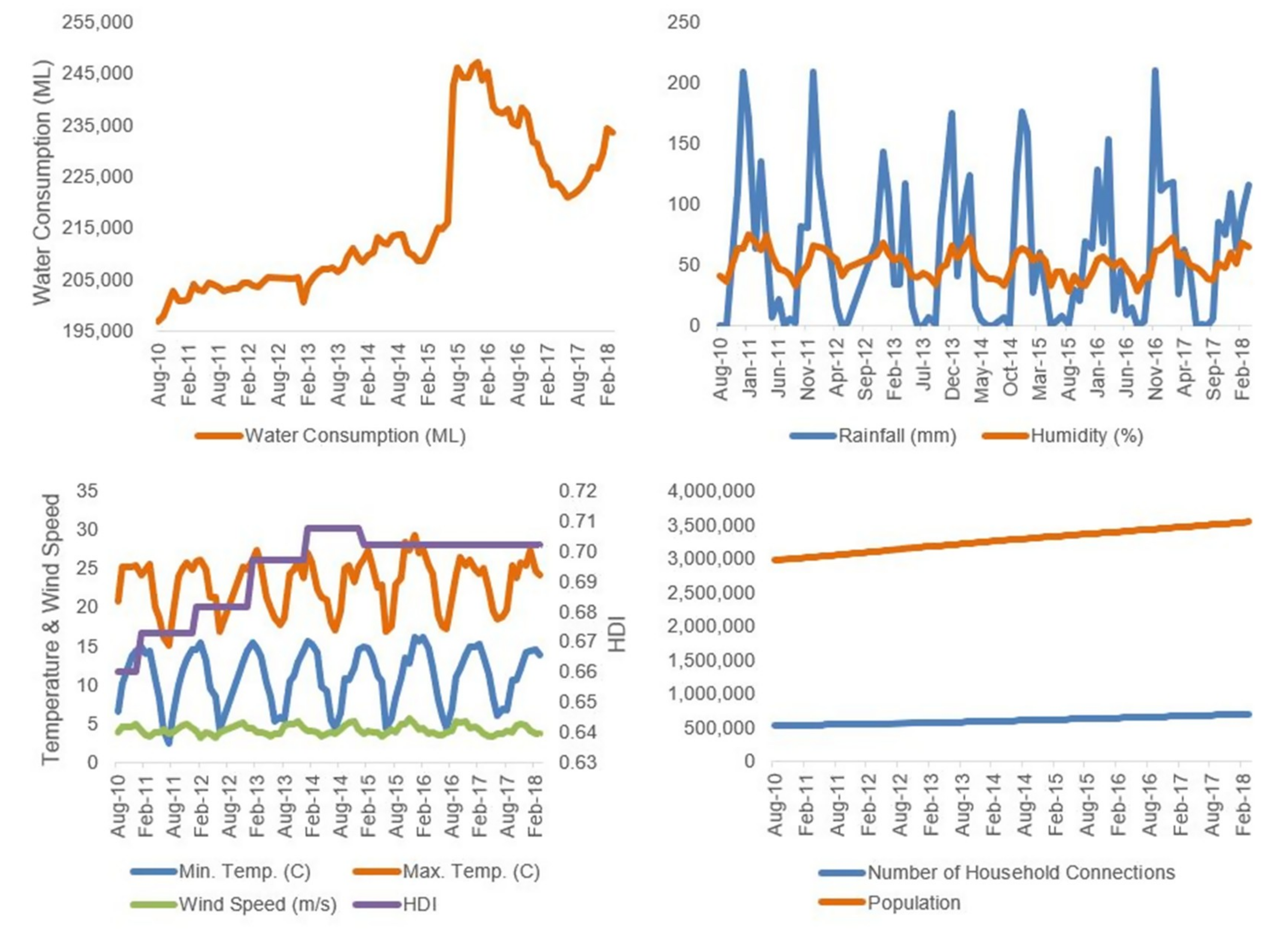
3. Description of Study Area

In this study, the City of Ekurhuleni (a metropolitan municipality), located in the Gauteng province of South Africa, was used as a case study (Figure 3). Gauteng is the most populated province in South Africa, with a population of approximately 14.7 million [37]. The City of Ekurhuleni was established in 2000 when Kyalami Metropolitan and the Eastern Gauteng Services Council were amalgamated (Figure 3). The city accounts for about 26% of Gauteng’s population, and as at 2016, it contributed 8.8% to South Africa’s gross added value. The human development index (HDI) of the city is 0.704. This is greater than the national value (0.653). Currently, the city is an epicenter of migration, and this has increased pressure on its water resources [38]. To address this problem, Gauteng province imports water from the Lesotho highlands [38].

Table 1. Ekurhuleni water infrastructure parameters [39].

Parameters	Values
Number of reservoirs	73
Number of towers	32
Number of bulk connections	186
Pipes (km)	11,448
Number of distribution zones	124
Population (million, 2016)	3.5
Annual population growth	2.51%

provides current figures relevant to the City of Ekurhuleni water infrastructure.

This city management seeks to ensure that Ekurhuleni transitions from being a fragmented city to being a “delivering city” from 2012 to 2020, a “capable city” from 2020 to 2030, and lastly a “sustainable city” from 2030 to 2055 [38]. To achieve these milestones, a long-term development strategy—the Ekurhuleni Growth and Development Strategy 2055 (GDS 2055)—has been developed to systematically analyze Ekurhuleni’s history and its development challenges. The document outlines the city’s desired growth and development trajectory. Urban integration and continued investment in water infrastructure is one of their strategic objectives. This is critical to attaining the state of a “sustainable city” and realizing the African Union Agenda 2063 and 2030 UN Sustainable Development Goals (SDGs)—which includes access to clean water and sanitation, innovation and infrastructure as well as reduced inequality. A reliable long-term water demand forecasting model which considers not only population, but other factors related to the weather and socio-economic profile of this city is required. This would assist in the planning and management of this city’s water resources, thereby fostering the achievement of its objectives.

Considering the city’s water infrastructure profile and its associated challenges, its water network is, therefore, considered as representative and relevant for use as a case study. To apply the models discussed in Section 2, the explanatory variables that directly and indirectly influence water demand were identified. Detail on key explanatory variables that affects water demand forecasting is available in Reference [21]. The current study considered rainfall $\left(R\right)$, minimum and maximum temperatures ($T_{min}$ and $T_{max}$), relative humidity $\left(RH\right)$, wind speed $\left(WS\right)$, number of household connections $\left(HH\right)$, population $\left(P\right)$, human development index $\left(HDI\right)$ and water consumption $\left(WC\right)$ as the explanatory variables.

Data sets for these variables, from August 2010 to March 2018, were obtained from the South African Weather Service, Statistics South Africa (Stats SA) and the City of Ekurhuleni. Water consumption data were based on billed water consumption, while weather information was obtained from a weather station at OR Tambo International Airport. In this study, the number of household connections provided an indication of the number of dwelling units served by the authority while population represented the total number of people domiciled in the study area. HDI is a measure of the city’s overall achievement in its socio-economic dimensions including life expectancy, education and income levels. This study used linear interpolation to transformed yearly population data into monthly values. Population records for the case study were based on the Stats SA report, and its annual HDI figures were, however, kept constant throughout the twelve months of the year.

Table 2. Descriptive statistics of data used in the study.

Statistical Parameter	$\mathit{R}$ (mm)	${\mathit{T}}_{\mathit{m}\mathit{i}\mathit{n}}$ (°C)	${\mathit{T}}_{\mathit{m}\mathit{a}\mathit{x}}$ (°C)	$\mathit{R}\mathit{H}$ (%)	$\mathit{W}\mathit{S}$ (m/s)	$\mathit{H}\mathit{H}$	$\mathit{P}$	$\mathit{H}\mathit{D}\mathit{I}$	$\mathit{W}\mathit{C}$$\left(\mathbf{M}\mathit{\ell }\right)$
Mean	59.37	11.11	23.15	51.10	4.19	607,096	3,280,134	0.69	216,917
Maximum	210.00	16.20	29.40	75.07	5.60	698,407	3,543,077	0.71	247,135
Minimum	-	2.50	15.10	28.07	3.23	526,700	2,975,216	0.66	196,908
Standard Deviation	59.42	3.65	3.38	11.56	0.58	50,953	165,046	0.01	14,524
Kurtosis coefficient	−0.30	−0.91	−0.72	−0.87	−0.64	−1.21	−1.12	0.01	−0.86
Skewness coefficient	0.81	−0.55	−0.60	0.07	0.48	0.12	−0.21	−1.15	0.70

and Figure 4 contain the statistical properties and historical trends of the data collected, respectively, for the case study. Between mid-2015 and March 2018, a surge in water consumption and variations were observed. The city’s water services planning manager attributed this change in trend to the installation of new water meters and repair of faulty water pipes. This maintenance works has led to an increase in revenue due to drastic reduction in water theft and leaks.

4. Model Development

The preliminary stage of model development often involves subjecting potential explanatory variables to a screening process. This is to ensure that only input variables that can provide a good representation of the system are included in a predictive model. When explanatory variables are screened properly, it improves predictive models’ learning process and consequently results in good generalization [40]. To test the above assertions, this study employed two scenarios for model development. The first scenario, which was referred to as “baseline Scenario”, involved the use of all potential explanatory variables (as per collected data) that could influence water consumption. The functional relationship that governed the baseline Scenario was expressed as:

$$WC=f\left(R, T_{min}, T_{max}, RH, WS, HH,P,HDI\right).$$

(10)

The second scenario, which was referred to as “Scenario 2”, used correlation analysis (based on Pearson correlation) to determine the dependencies between the potential explanatory variables and water consumption.

Table 3. Results of correlation analysis.

Potential Explanatory Variables	Target Variable (WC)
$R$	−0.06
$T_{min}$	0.07
$T_{max}$	0.15
$RH$	−0.23
$WS$	0.50
$HH$	0.79
$P$	0.79
$HDI$	0.59

presents the correlation analysis results. A correlation coefficient of 0.5 was adopted as the cut-off point. The results obtained showed a high correlation (≥0.5) between number of household connections, population, human development index and wind speed, while other potential explanatory variables produced lower correlation coefficients and were therefore discarded. The functional relationship that governed the development of Scenario 2 models was expressed as:

$$WC=f\left(HH,P,HDI,WS\right).$$

(11)

The data sets were split into two subsets of similar statistical properties for both scenarios; 70% of the data (61 samples) used for model training and 30% (26 samples) for validation [41,42].

The modeling of the water consumption in the City of Ekurhuleni was based on four modeling techniques—MLR, ES, ANN and SVM. As earlier stated, two ANN models were developed. The first ANN, which was referred to as ANN–CG, was trained using a CG algorithm while the second (ANN–DE) was trained using an EC technique—the classic DE developed by Reference [43]. The training of the ANN using the DE algorithm was implemented using Visual Basic for Applications (VBA) programming language on an Intel Core i7 PC with 2.70 GHz and 16 GB RAM. The SVM, ANN–CG and MLR models were implemented using DTREG platform [44], while ES was implemented using the Data Analysis Tool pack in Microsoft Excel. Hence, a total of five modeling approaches namely MLR, ES, ANN–CG, ANN–DE and SVM were implemented in this study. Four of the modeling approaches (MLR, ANN–CG, ANN–DE and SVM) were implemented for the two scenarios described in Equations (10) and (11) and their performance tested against ES.

Table 4. Summary of key information used for model development.

MLR	ES	ANN–CG	ANN–DE	SVM
Confidence interval: 95%	Optimization of damping factor: (0.1, 0.9) Incremental function: 0.1	Model type: Multilayer Perceptron Number of network layers: 3 (1 hidden) Optimization of hidden layer neurons: (1, 10) Stepping function: 1 Overfitting prevention: Hold out 20% of training rows Hidden layer activation function: Logistic Output layer activation function: Linear CG Parameters: Convergence tries: 4 Maximum iterations: 10,000 Iterations without improvement: 100 Convergence tolerance: 1 × 10−5 Minimum improvement delta: 1 × 10−5 Minimum gradient: 1 × 10−5 Training method: Scaled-conjugate gradient	Model type: Multilayer Perceptron Number of network layers: 3 (1 hidden) Optimization of hidden layer neurons: (1, 10) Stepping function: 1 Overfitting prevention: Yes, Early stopping Hidden layer activation function: Logistic-sigmoidal (0, 1) and re-scaling of inputs: (0.1, 0.9) Output layer activation function: Linear DE Parameters: Pop. Size, $NP=D \times 10$ where $D$ = number of weights and biases Sensitivity analysis: Yes Crossover rate, $CR$: (0.5, 0.9) interval Mutation rate, $F$: (0.5, 0.9) interval Stepping value for $CR$ and $F$: 0.1 Number of generations: 1000	Model type: Epsilon SVR Kernel function: RBF Stopping criteria: 0.001 Parameter optimization: Grid search: (10, 1) Pattern search: Intervals: 10 Tolerance: 1 × 10−8 % rows to use for search: 100 Cross-validate: 4 folds Model Parameters: C: (0.1, 5000) Gamma: (0.1, 50) P: (0.0001, 100)

presents the summary of key information that governs the predictive models. The ANN network weights and bias were updated concurrently during the implementation.

5. Model Evaluation

This study used three statistical measures, root mean-square error (RMSE), mean absolute percent error (MAPE) and coefficient of determination (R²), to evaluate the performance of the predictive models. The RMSE is a measurement of the error variance in the model prediction, while the MAPE scores the absolute differences between observed and predicted output values [45]. R² measures the degree of collinearity between observed values and predicted values, thereby defining the proportion of variance in observed values as explained by the models. RMSE and MAPE values indicate a better model as their values approach 0, while a R² value indicates a better model as its value approaches 1. Equations (12)–(14) give the mathematical expressions for these measures.

$$\mathrm{RMSE}=\sqrt{\frac{{{\displaystyle \sum }}_{i=1}^N{(O_i-P_i)}^2}{N}},$$

(12)

$$\mathrm{MAPE}=100\frac{1}{N}{{\displaystyle \sum }}_{I=1}^N\frac{\left|O_i-P_i\right|}{O_i},$$

(13)

$$R^2={\left[\frac{{{\displaystyle \sum }}_{i=1}^N\left(O_i-\overline{O}\right)\left(P_i-\tilde{P}\right)}{\sqrt{{{\displaystyle \sum }}_{i=1}^N{\left(O_i-\overline{O}\right)}^2\times {{\displaystyle \sum }}_{i=1}^N{\left(P_i-\tilde{P}\right)}^2}}\right]}^2,$$

(14)

where $N$ is the number of instances in the set, and $P_i$, $O_i$, $\tilde{P}$ and $\overline{O}$ are the predicted and observed values, and their respective average values.

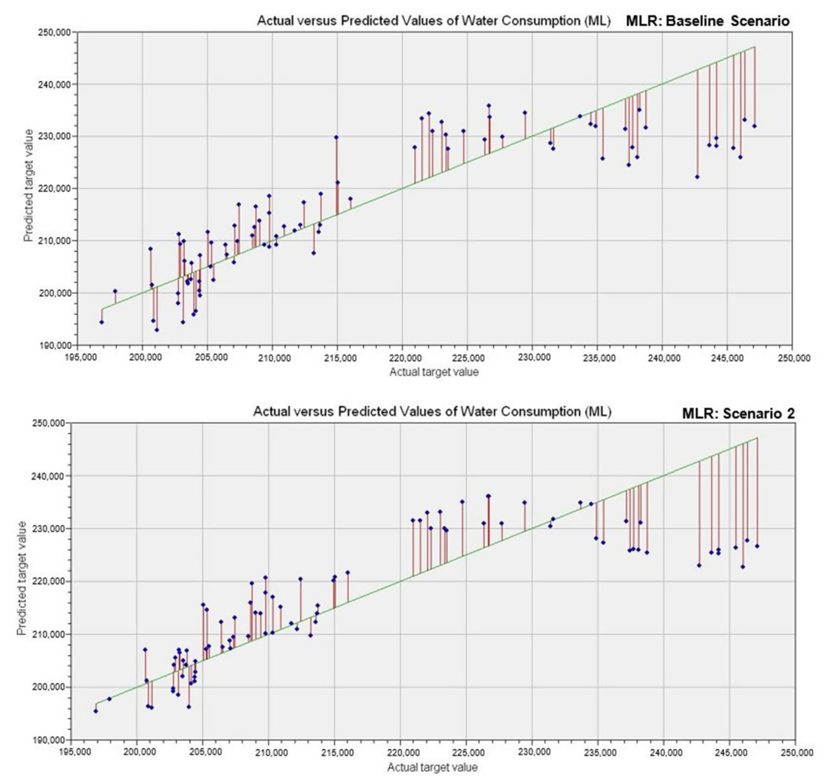
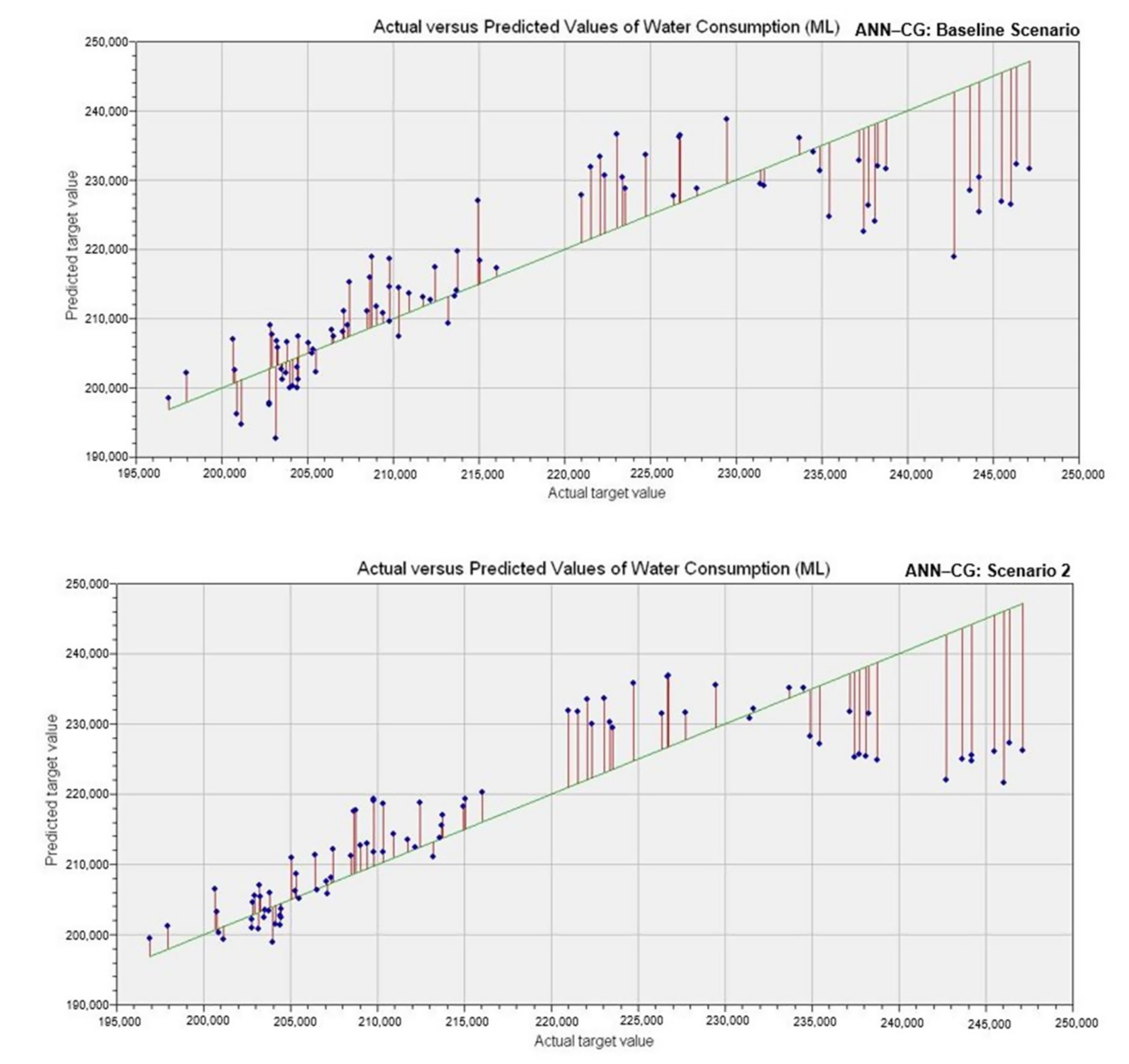
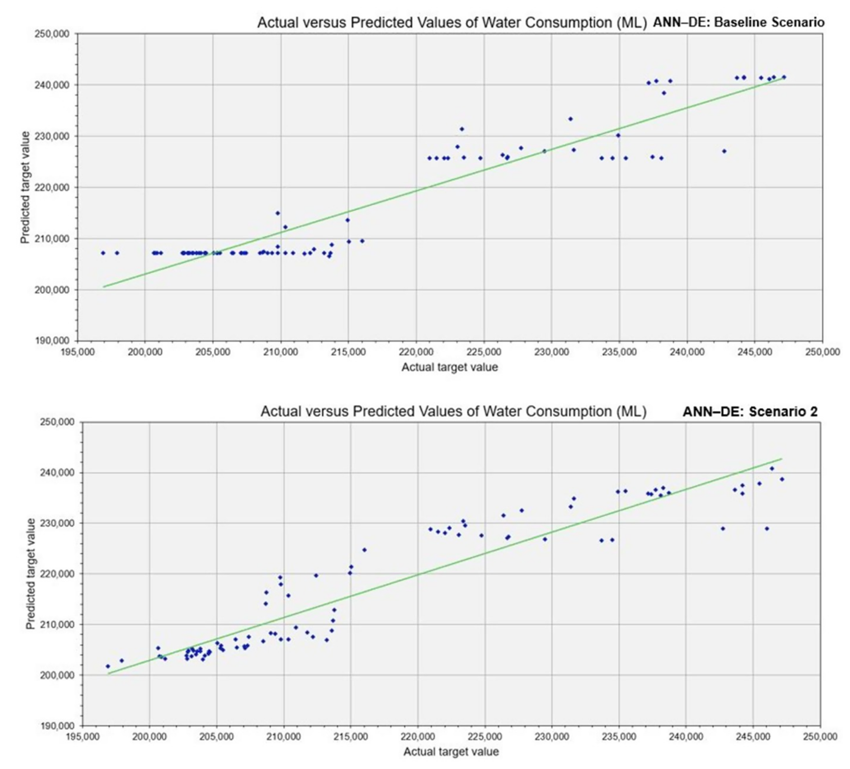
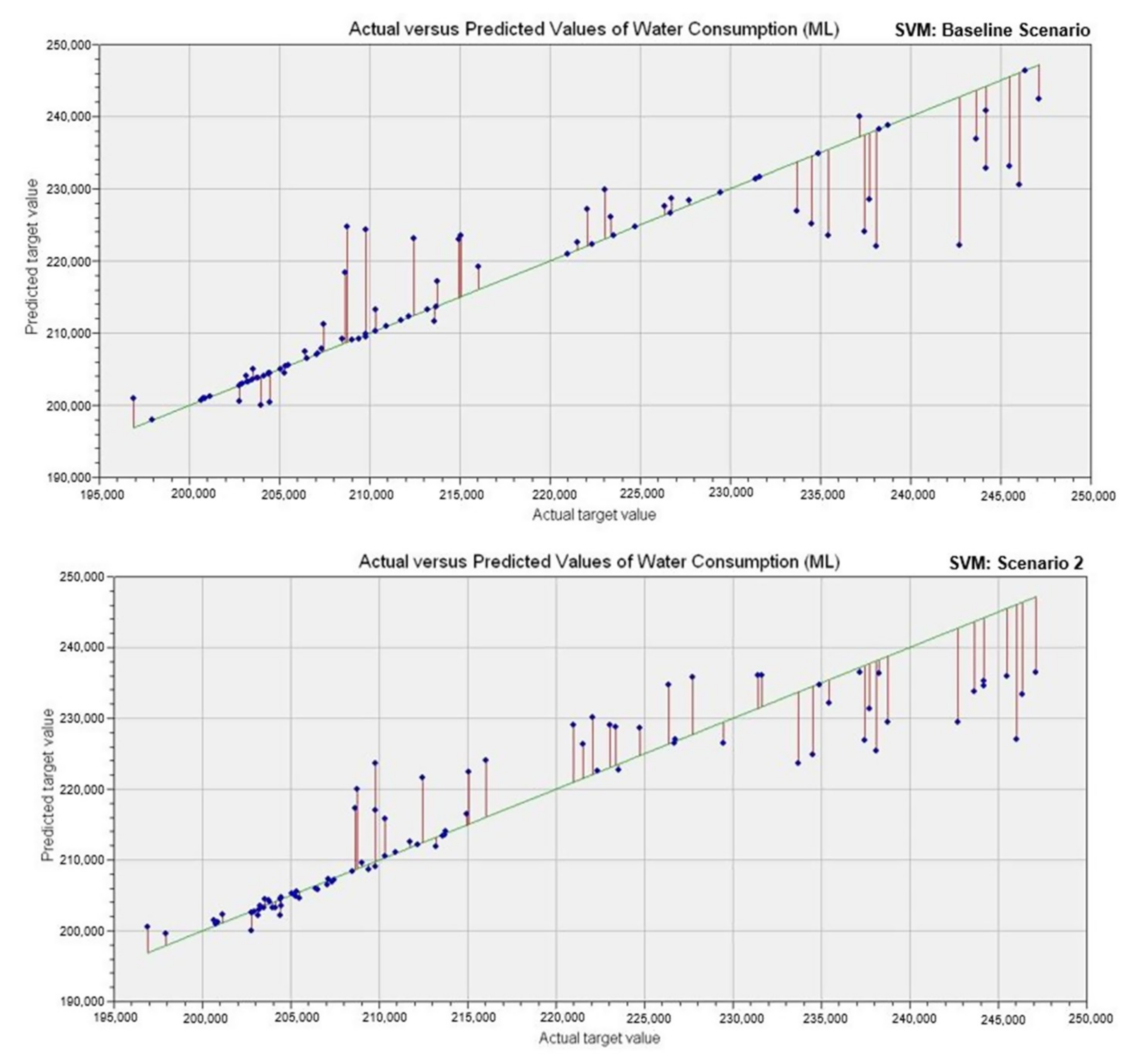
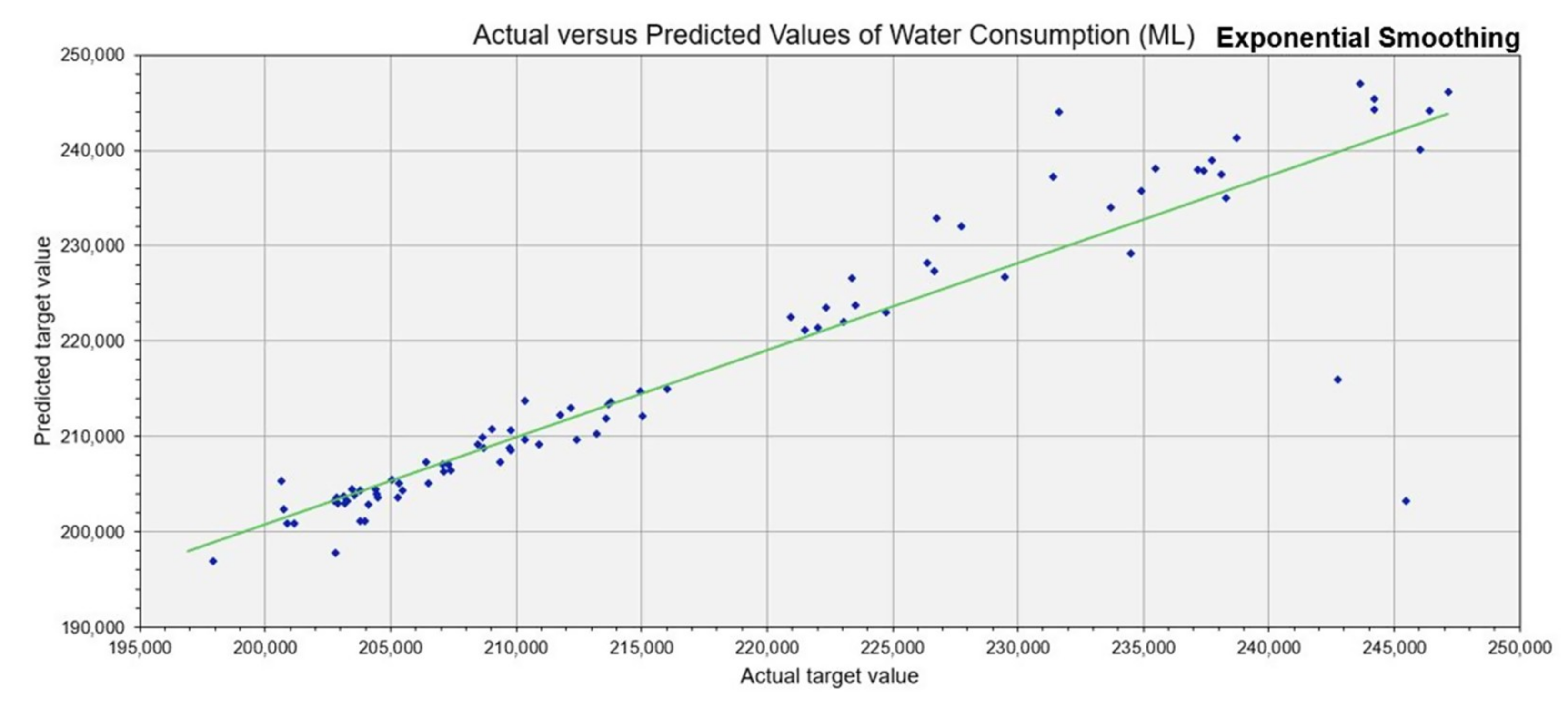
6. Result and Discussions

Table 5. Performance of models developed for baseline Scenario.

Baseline	Training	Testing	Training	Testing	Training	Testing
Techniques	R2	R2	RMSE	RMSE	MAPE	MAPE
MLR	0.7268	0.7030	7449	8107	2.6699	2.7181
ANN–CG	0.7236	0.6614	7492	8655	2.5906	2.7959
ANN–DE	0.9038	0.8576	4766	5160	1.7892	1.8398
SVM	0.8842	0.7568	4850	7336	0.9789	2.2359

and

Table 6. Performance of models developed for Scenario 2.

Optimal Dataset	Training	Testing	Training	Testing	Training	Testing
Techniques	R2	R2	RMSE	RMSE	MAPE	MAPE
MLR	0.6765	0.7201	8106	7430	2.6823	2.4282
ANN–CG	0.6835	0.7122	8017	7507	2.5472	2.4490
ANN–DE	0.8812	0.9233	5092	4172	1.6650	1.5090
SVM	0.8609	0.8678	5315	5296	1.8775	1.6655

present the predictive models’ performance for the baseline Scenario and Scenario 2, respectively. The results for the baseline Scenario show satisfactory performance during training, but they suffered from overfitting during testing. When the models’ performance was compared—without considering overfits,—the ANN–DE model produced the lowest RMSE (5160 Mℓ) and MAPE (1.8%) values as well as the highest R² (0.8576) value. The ranking order, in term of performance, for this scenario was ANN–DE > SVM > MLR > ANN–CG. The ANN–DE and conventional MLR models produced the lowest performance differences (percentage overfits) between the training and testing phases, but the MLR model had a slight edge over the ANN–DE models in terms of R² and MAPE. The percentage overfit is mathematically expressed as:

$$\mathrm{Percentage}\mathrm{overfit}=\frac{P_t-P_v}{P_t}\times 100,$$

(15)

where $P_t$ is the value of the performance metric observed during training while $P_v$ is the value of the performance metric observed during validation.

The percentage overfit produced by the ANN–DE model were 5.4%, 8.3% and 2.8% for R², RMSE and MAPE, respectively, while the MLR produced 3.4%, 8.8% and 1.8% for R², RMSE and MAPE, respectively. The SVM model had the highest percentage overfit: 16.8%, 51.2% and 128.4% for R², RMSE and MAPE, respectively. Figure 5, Figure 6, Figure 7 and Figure 8 further illustrate performance of the baseline Scenario models wherein some degree of under- and over-estimations can be observed. Generally, the overfitting problems encountered in the baseline Scenario suggest that some of the explanatory variables considered were irrelevant or redundant in determining the water consumption profile for the City of Ekurhuleni. Conversely, the exclusion of the explanatory variables in Scenario 2 was responsible for its improved performance.

In Scenario 2, it can be observed that the learning accuracies of all the models are superior to those obtained in the baseline scenario. The percentage improvements for the predictive models range from 7–15%, 9–39% and 12–34% for R², RMSE and MAPE, respectively. These results show that all models produced in Scenario 2 were more generalized and not plagued by overfitting. Figure 5, Figure 6, Figure 7 and Figure 8 show that the data points were much closer to the line of equality than that of the baseline Scenario. These improvements in the predictive models’ performance suggest that the adoption of correlation analysis was successful in finding the optimal subset of input variables required to model the water consumption data. Remarkably, the optimal subset comprising four input variables ($HH,P,HDI,WS$) were good enough to adequately represent the water consumption profile of the city as opposed to eight variables used in the baseline scenario. This implies that the over-parameterization effects were avoided in the Scenario 2 models by incorporating a screening technique. The performance metrics for Scenario 2 models are presented in Table 6. The ANN–DE model produced the lowest error (4172 Mℓ and 1.5% for RMSE and MAPE, respectively), as well as highest R² (0.9233) value. The SVM model has the second-best performance; its R², RMSE, and MAPE values were 0.8678, 5296 Mℓ and 1.7%, respectively. The conventional MLR—which was the third best model—R², RMSE and MAPE values were 0.7201, 7430 Mℓ and 2.4%, respectively. And lastly, the ANN–CG models R², RMSE and MAPE values were 0.7122, 7507 and 2.4%, respectively.

Table 7. Performance of models developed using exponential smoothing.

Optimal Dataset	Training	Testing	Training	Testing	Training	Testing
Techniques	R2	R2	RMSE	RMSE	MAPE	MAPE
ES	0.9038	0.6103	4348	8682	0.9458	1.3188

and Figure 9 present results obtained from the ES technique which was implemented by varying the damping factor between 0.1 and 0.9 with an incremental function of 0.1. Our investigation showed that a damping factor of 0.1, the optimal damping factor, yielded the least error estimates. The performance indices presented in Table 7 show a remarkable model performance during the training; however, the performance depreciated during the testing phase; this was caused by overfitting. The percentage overfit values of the ES model were 32.5%, 99.7% and 39.4% for R², RMSE and MAPE, respectively. Based on these observations, it can be inferred that the ANN–DE model (developed in Scenario 2) was better than the ES model because it was not plagued by overfitting problem. This observation further demonstrated the efficacy of evolutionary-based soft computing techniques over conventional methods, such as time series analysis and linear regression-based methods.

A comparative evaluation of the architecture of the ANN models showed that the ANN–DE model exhibited lesser complexity compared to the ANN–CG model. Upon varying the number of hidden layer neurons in each of the ANN models between one and 10, the optimal architecture for the ANN–CG models comprised nine hidden layer neurons, while the ANN–DE model comprised only four hidden layer neurons. This implies that the computational time of the ANN–CG model would be higher than that of the ANN–DE model. It is interesting to note that the ANN–DE model, with lesser complex architecture and lower computational demand and time, achieved a higher degree of accuracy than the ANN–CG model. This observation was consistent with the results reported by Adeyemo, Oyebode and Stretch [8].

The techniques used in this study further confirmed the robustness and applicability of EC techniques in water demand forecasting and their ability to effectively account for the complex interactions between water use and long-term effects of climate and socio-economic parameters. It can be deduced that potential exists in using EC-inspired models to plan and manage water resources. Although the AI and EC techniques implemented in this study were done at a monthly temporal scale, it is accepted that the performance of these techniques will be consistent when subjected to data at finer temporal scales. This is because, research has shown that once a data set for a prediction problem is from the same domain, an ANN model performance will not be affected by changes in temporal scale [46]. This consistency is due to the normalization or re-scaling of data inputs (typically between 0 and 1) that is embedded in the ANN modeling algorithm [46]. Investigation of the impacts of seasonality on water demand using EC techniques is however recommended as this will ensure that the influence of seasonal variation and its sensitivity to water demand (often associated with climatic and socioeconomic factors) are well-catered for. Future research should also focus on extending the use of EC techniques to assess the impacts of nature-based solutions as well as water conservation and reuse strategies on water demand. These may include simulating the impacts of the use of water efficient appliances, consumer behavior and alternative water sources.

7. Conclusions

This study compared the performance of soft computing techniques (ANN–CG, ANN–DE and SVM) with ES and MLR as predictive models for water consumption. Real-world data sets, from the City of Ekurhuleni, South Africa, were used to compare these models’ performance (R², RMSE and MAPE). The data sets were used to create two scenarios to understand the effects of input parameters on water consumption forecasting. The first scenario, which was referred to as the baseline Scenario, used potential explanatory variables to forecast water consumption, while the second used correlation analysis to reduce the potential explanatory variables. The results from the first scenario suffered from overfitting problem when they were compared with training data sets; on the other hand, models from second scenario did not have this problem.

During the scenarios’ analysis, it was observed that the ANN–DE model performed better than the other predictive models. The order of the predictive models’ performance was ANN–DE > SVM > MLR > ANN–CG. This study results showed that the ANN–DE model’s performance was better than ES results—a standard time series model. In terms of learning, the DE algorithm performed better than the CG algorithm; in addition, it produced a less complex network architecture. Thus, this study has, therefore, proved that the integration of evolutionary computation techniques into ANN model is beneficial to the water demand modeling community. Future research can investigate the performance of the ANN–DE model with larger data sets when available. Future research can also consider the use of special algorithms, such as Bayesian optimization, for model architecture determination and hyperparameter configuration.

References

1. UNESCO. The United Nations World Water Development Report 2015: Water for a Sustainable World; United Nations World Water Assessment Programme—WWAP; 9231000713; UNESCO: Paris, France, 2015. [Google Scholar]
2. Pulido-Calvo, I.; Montesinos, P.; Roldán, J.; Ruiz-Navarro, F. Linear regressions and neural approaches to water demand forecasting in irrigation districts with telemetry systems. Biosyst. Eng. 2007, 97, 283–293. [Google Scholar] [CrossRef]
3. House-Peters, L.A.; Chang, H. Urban water demand modeling: Review of concepts, methods, and organizing principles. Water Resour. Res. 2011, 47. [Google Scholar] [CrossRef] [Green Version]
4. Donkor, E.A.; Mazzuchi, T.A.; Soyer, R.; Alan Roberson, J. Urban water demand forecasting: Review of methods and models. J. Water Resour. Plan. Manag. 2012, 140, 146–159. [Google Scholar] [CrossRef]
5. Shabani, S.; Yousefi, P.; Adamowski, J.; Naser, G. Intelligent soft computing models in water demand forecasting. In Water Stress in Plants; Rahman, I.M.M., Begum, Z.A., Hasegawa, H., Eds.; InTech: Rijeka, Croatia, 2016. [Google Scholar]
6. UNESCO. The United Nations World Water Development Report 2016: Water and Jobs—Facts and Figures; United Nations World Water Assessment Programme—WWAP; 9231002015; UNESCO: Paris, France, 2016. [Google Scholar]
7. Ghalehkhondabi, I.; Ardjmand, E.; Young, W.A.; Weckman, G.R. Water demand forecasting: Review of soft computing methods. Environ. Monit. Assess. 2017, 189, 313. [Google Scholar] [CrossRef] [PubMed]
8. Adeyemo, J.; Oyebode, O.; Stretch, D. River Flow Forecasting Using an Improved Artificial Neural Network. In EVOLVE-A Bridge Between Probability, Set Oriented Numerics, and Evolutionary Computation VI; Tantar, A.-A., Tantar, E., Emmerich, M., Legrand, P., Alboaie, L., Luchian, H., Eds.; Springer: Cham, Switzerland, 2018; pp. 179–193. [Google Scholar]
9. Ch, S.; Anand, N.; Panigrahi, B.K.; Mathur, S. Streamflow forecasting by SVM with quantum behaved particle swarm optimization. Neurocomputing 2013, 101, 18–23. [Google Scholar] [CrossRef]
10. Soltani, F.; Kerachian, R.; Shirangi, E. Developing operating rules for reservoirs considering the water quality issues: Application of ANFIS-based surrogate models. Expert Syst. Appl. 2010, 37, 6639–6645. [Google Scholar] [CrossRef]
11. Dhungel, R.; Fiedler, F. Price elasticity of water demand in a small college town: An inclusion of system dynamics approach for water demand forecast. Air Soil Water Res. 2014, 7, ASWR-S15395. [Google Scholar] [CrossRef]
12. Olofintoye, O.; Otieno, F.; Adeyemo, J. Real-time optimal water allocation for daily hydropower generation from the Vanderkloof dam, South Africa. Appl. Soft Comput. 2016, 47, 119–129. [Google Scholar] [CrossRef]
13. Adamowski, J.; Karapataki, C. Comparison of multivariate regression and artificial neural networks for peak urban water-demand forecasting: Evaluation of different ANN learning algorithms. J. Hydrol. Eng. 2010, 15, 729–743. [Google Scholar] [CrossRef]
14. Ji, G.; Wang, J.; Ge, Y.; Liu, H. Urban water demand forecasting by LS-SVM with tuning based on elitist teaching-learning-based optimization. In Proceedings of the 26th Chinese Control and Decision Conference (2014 CCDC), Changsha, China, 31 May–2 June 2014; pp. 3997–4002. [Google Scholar]
15. Vijayalaksmi, D.; Babu, K.J. Water supply system demand forecasting using adaptive neuro-fuzzy inference system. Aquat. Procedia 2015, 4, 950–956. [Google Scholar] [CrossRef]
16. Varahrami, V. Application of genetic algorithm to neural network forecasting of short-term water demand. In Proceedings of the International Conference on Applied Economics—ICOAE, Milan, Italy, 4–6 July 2019; pp. 783–787. [Google Scholar]
17. Wu, Z.Y.; Yan, X. Applying genetic programming approaches to short-term water demand forecast for district water system. In Water Distribution Systems Analysis 2010; Lansey, K.E., Choi, C.Y., Ostfeld, A., Pepper, I.L., Eds.; American Society of Civil Engineers (ASCE): Reston, VA, USA, 2010; pp. 1498–1506. [Google Scholar]
18. Zhai, C.; Zhang, H.; Zhang, X. Application of system dynamics in the forecasting water resources demand in Tianjin polytechnic university. In Proceedings of the International Conference on Artificial Intelligence and Computational Intelligence (AICI ‘09), Shanghai, China, 7–8 November 2009; pp. 273–276. [Google Scholar]
19. Ali, A.M.; Shafiee, M.E.; Berglund, E.Z. Agent-based modeling to simulate the dynamics of urban water supply: Climate, population growth, and water shortages. Sustain. Cities Soc. 2017, 28, 420–434. [Google Scholar] [Green Version]
20. Oyebode, O.; Stretch, D. Neural network modeling of hydrological systems: A review of implementation techniques. Nat. Resour. Modeling 2018. [Google Scholar] [CrossRef]
21. Oyebode, O.; Babatunde, D.E.; Monyei, C.G.; Babatunde, O.M. Water demand modelling using evolutionary computation techniques: Integrating water equity and justice for realization of the sustainable development goals. Heliyon 2019. in review. [Google Scholar]
22. Polebitski, A.S.; Palmer, R.N. Seasonal residential water demand forecasting for census tracts. J. Water Resour. Plan. Manag. 2009, 136, 27–36. [Google Scholar] [CrossRef]
23. Toriman, E.; Jaafar, O.; Maru, R.; Arfan, A.; Ahmar, A.S. Daily Suspended Sediment Discharge Prediction Using Multiple Linear Regression and Artificial Neural Network. J. Phys. Conf. Ser. 2018, 954, 012030. [Google Scholar] [Green Version]
24. Su, Y.; Gao, W.; Guan, D.; Su, W. Dynamic assessment and forecast of urban water ecological footprint based on exponential smoothing analysis. J. Clean. Prod. 2018, 195, 354–364. [Google Scholar] [CrossRef]
25. Hyndman, R.; Koehler, A.B.; Ord, J.K.; Snyder, R.D. Forecasting with Exponential Smoothing: The State Space Approach; Springer Science & Business Media: Berlin/Heidelberg, Germany, 2008. [Google Scholar]
26. Tomić, A.Š.; Antanasijević, D.; Ristić, M.; Perić-Grujić, A.; Pocajt, V. Application of experimental design for the optimization of artificial neural network-based water quality model: A case study of dissolved oxygen prediction. Environ. Sci. Pollut. Res. 2018, 25, 9360–9370. [Google Scholar] [CrossRef]
27. Shahin, M.A.; Jaksa, M.B.; Maier, H.R. State of the art of artificial neural networks in geotechnical engineering. Electron. J. Geotech. Eng. 2008, 8, 1–26. [Google Scholar]
28. Mafi, S.; Amirinia, G. Forecasting hurricane wave height in Gulf of Mexico using soft computing methods. Ocean Eng. 2017, 146, 352–362. [Google Scholar] [CrossRef]
29. Ilonen, J.; Kamarainen, J.-K.; Lampinen, J. Differential evolution training algorithm for feed-forward neural networks. Neural Process. Lett. 2003, 17, 93–105. [Google Scholar] [CrossRef]
30. Hanke, M. Conjugate Gradient Type Methods for Ill-Posed Problems, 1st ed.; Routledge: New York, NY, USA, 2017; p. 144. [Google Scholar]
31. Technosoft, M. Artificial Neural Network. Available online: https://msatechnosoft.in/blog/tech-blogs/artificial-neural-network-types-feed-forward-feedback-structure-perceptron-machine-learning-applications (accessed on 20 November 2018).
32. Vapnik, V.N. An overview of statistical learning theory. IEEE Trans. Neural Netw. 1999, 10, 988–999. [Google Scholar] [CrossRef] [PubMed]
33. Elshorbagy, A.; Corzo, G.; Srinivasulu, S.; Solomatine, D. Experimental investigation of the predictive capabilities of data driven modeling techniques in hydrology-Part 1: Concepts and methodology. Hydrol. Earth Syst. Sci. 2010, 14, 1931–1941. [Google Scholar] [CrossRef]
34. Oyebode, O.K.; Otieno, F.A.O.; Adeyemo, J. Review of three data-driven modelling techniques for hydrological modelling and forecasting. Fresenius Environ. Bull. 2014, 23, 1443–1454. [Google Scholar]
35. Karimi, S.; Shiri, J.; Kisi, O.; Shiri, A.A. Short-term and long-term streamflow prediction by using wavelet–gene expression programming approach. Ish J. Hydraul. Eng. 2016, 22, 148–162. [Google Scholar] [CrossRef]
36. Vapnik, V. The Nature of Statistical Learning Theory; Springer Science & Business Media: New York, NY, USA, 2013. [Google Scholar]
37. Statistics South Africa—Stats SA. Statistical Release P0302: Mid-Year Population Estimates 2018; Statistics South Africa: Pretoria, South Africa, 2018. [Google Scholar]
38. IDP. Integrated Development Plan of City of Ekurhuleni 2017/2018 to 2020/2021; City of Ekurhuleni: Ekurhuleni, South Africa, 2018. [Google Scholar]
39. Gubuza, D. Water Conservation and Water Demand Management in the City of Ekurhuleni: On-Site Leak Repair. Presented at Rand Water Services Forum, Johannesburg, South Africa, 24 May 2017. [Google Scholar]
40. Bowden, G.J.; Dandy, G.C.; Maier, H.R. Input determination for neural network models in water resources applications. Part 1—background and methodology. J. Hydrol. 2005, 301, 75–92. [Google Scholar] [CrossRef]
41. Storn, R.; Price, K. Differential evolution–a simple and efficient heuristic for global optimization over continuous spaces. J. Glob. Optim. 1997, 11, 341–359. [Google Scholar] [CrossRef]
42. Wanjawa, B.W.; Muchemi, L. Ann Model to Predict Stock Prices at Stock Exchange Markets. arXiv 2014, arXiv:1502.06434. [Google Scholar]
43. Rau, H.H.; Hsu, C.Y.; Lin, Y.A.; Atique, S.; Fuad, A.; Wei, L.M.; Hsu, M.H. Development of a web-based liver cancer prediction model for type II diabetes patients by using an artificial neural network. Comput. Methods Programs Biomed. 2016, 125, 58–65. [Google Scholar] [CrossRef] [PubMed]
44. Sherrod, P.H. DTREG Predictive Modeling Software. Available online: http://www.dtreg.com (accessed on 20 November 2018).
45. Amaranto, A.; Munoz-Arriola, F.; Corzo, G.; Solomatine, D.P.; Meyer, G. Semi-seasonal groundwater forecast using multiple data-driven models in an irrigated cropland. J. Hydroinformatics 2018. [Google Scholar] [CrossRef]
46. Engelbrecht, A.P. Computational Intelligence: An Introduction; John Wiley & Sons: West Sussex, UK, 2007. [Google Scholar]
Figure 1. Typical structure of a feedforward artificial neural network (ANN) [31].
Resources 08 00156 g001
Figure 2. Graphical illustration of support vector machine (SVM) working principles [28].
Resources 08 00156 g002
Figure 3. Overview of Ekurhuleni Metropolitan Municipality Service Area.
Resources 08 00156 g003
Figure 4. Historical trend of variables considered for model development.
Resources 08 00156 g004
Figure 5. Scatter plots of observed and multiple linear regression (MLR)-predicted water demand for both scenarios.
Resources 08 00156 g005
Figure 6. Scatter plots of observed and ANN–conjugate gradient (CG)-predicted water demand for both scenarios.
Resources 08 00156 g006
Figure 7. Scatter plots of observed and ANN–differential evolution (DE)-predicted water demand for both scenarios.
Resources 08 00156 g007
Figure 8. Scatter plots of observed and SVM-predicted water demand for both scenarios.
Resources 08 00156 g008
Figure 9. Scatter plots of observed and exponential smoothing (ES)-predicted water demand.
Resources 08 00156 g009