Article

Regression Model to Predict the Higher Heating Value of Poultry Waste from Proximate Analysis

1
Industrial and Systems Engineering Department, Morgan State University, 1700 East Cold Spring Lane, Baltimore, MD 21251, USA
2
Center for Advanced Energy Systems and Environmental Technologies, School of Engineering, Morgan State University, 5200 Perring Parkway, Baltimore, MD 21239, USA
3
Department of Chemistry, Towson University, 8000 York Road, Towson, MD 21252, USA
*
Author to whom correspondence should be addressed.
Resources 2018, 7(3), 39; https://doi.org/10.3390/resources7030039
Submission received: 18 May 2018 / Revised: 12 June 2018 / Accepted: 23 June 2018 / Published: 26 June 2018

Abstract

:
Improper land application of excess poultry waste (PW) causes environmental issues and other problems. Meanwhile there is an increasing trend of using PW as an alternative energy resource. The Higher Heating Value (HHV) is critical for designing and analyzing the PW conversion process. Several proximate-based mathematical models have been proposed to estimate the HHV of biomass, coal, and other solid fuels. Nevertheless, only a small number of studies have focused on a subclass of fuels, especially for PW. The aim of this study is to develop proximate-based regression models for an HHV prediction of PW. Sample data of PW were collected from open literature to develop regression models. The resulting models were then validated by additional PW samples and other published models. Results indicate that the most accurate model contains linear (all proximate components), polynomial terms (quadratic and cubic of volatile matter), and interaction effect (fixed carbon and ash). Moreover, results show that best-fit regression model has a higher R2 (91.62%) and lower estimation errors than the existing proximate-based models. Therefore, this new regression model can be an excellent tool for predicting the HHV of PW and does not require any expensive equipment that measures HHV or elemental compositions.

1. Introduction

The increasing demand for animal and protein products (e.g., egg, meat) has led to a high number of animal feeding operations and massive quantities of poultry waste (PW) in confined areas [1]. PW from poultry farming includes a mixture of poultry manure (excreta), bedding materials (e.g., wood shavings, sawdust, straw, pine or rice husk), waste feed, dead birds, broken eggs, and feathers removed from poultry houses [2,3]. Poultry manure (or chicken manure) is an organic waste, mainly feces and urine of chicken, whereas poultry litter refers to a mixture of poultry manure, bedding materials, spilled feed and feathers [1]. In 2009, with the assumption of 1.4 ton of litter per 1000 birds, a total of about 25 million tons of poultry litter were generated in the USA and the EU [1]. Due to its rich nutrient contents, such as nitrogen, phosphorous, potassium, and calcium, most PW has traditionally been utilized as an organic fertilizer on agricultural land [1,2]. However, excess application of PW can lead to an overabundance of nutrients in the watershed, with a resulting eutrophication on water bodies and water pollutions (e.g., nitrate contamination). As a result, excess application of PW can pose a risk to the health of humans, animals, and the aquatic ecosystem [2,4]. Because of its energetic and superior fuel properties, PW is recognized as a biomass fuel and energy resource for alternative thermochemical conversion processes, namely composting, anaerobic digestion, combustion, gasification, and pyrolysis [2,5]. Among these alternative conversion technologies, combustion and co-combustion has been strongly suggested to be a cost-effective and environmentally-friendly disposal route for PW while providing an energy source for both space heating of poultry houses and large-scale power generation [2,3,4].
The design and operation of more efficient biomass combustion systems rely substantially on several fuel characteristics, namely heating value, moisture, ash content, and elemental composition [6,7]. The heating value (or calorific value) defines the energy content of fuel and is one of the most important fuel properties for achieving energy balance, engineering analysis, design calculations, and numerical simulations of thermal conversion systems [6,7,8]. The heating value is usually measured by the higher heating value (HHV) or lower heating value (LHV). HHV, also known as the gross calorific value or gross energy, refers to the heat released by the complete combustion of fuel, assuming that the water originally present in the fuel and any generated water are present in a condensed state [6,9]. LHV, also known as the net heating value, assumes that the water is present in a vapor state at the end of combustion and is determined by subtracting the latent heat of water vaporization from the HHV [10]. Experimentally, an adiabatic bomb calorimeter is used to measure the enthalpy change between reactants and products [6,11]. In a previous study, the HHV of PW samples from nine different farms was experimentally determined to vary between 12,052 and 13,882 kJ/kg [12]. An IKA C5003 bomb calorimeter was used in accordance with the Spanish Association for Standardization, UNE standard 164001EX [12]. Cotana et al. [13] also measured the HHV of two PW samples from different farming practices by using a LECO AC350 calorimeter, in compliance with UNI9017 standard. However, bomb calorimeters may not always be accessible to all laboratories. Additionally, experimental methods to measure the HHV are usually time consuming, complicated, and have higher possibilities of experimental errors [7,14,15].
Therefore, numerous mathematical models have been developed to predict the HHV of energy resources from results collected from ultimate analysis (or elemental analysis), proximate analysis, chemical analysis, and structural analysis [10,16]. Ultimate and proximate analyses provide basic fuel characterizations and are the most commonly used analyses to predict the HHV. Ultimate analysis measures the major elemental composition of samples, such as carbon (C), hydrogen (H), oxygen (O), nitrogen (N) and sulfur (S), in weight percentage (wt %) [7]. Sheng and Azevedo [6] found that mathematical models based on ultimate analysis are more accurate than models derived from proximate and chemical analyses because ultimate analysis quantifies elemental contents and provides a more detailed chemical composition of fuels. Yin et al. [7] also suggested that ultimate analysis-based models are more accurate than proximate analysis. But ultimate analysis requires expensive element analyzers as well as special experimental arrangements with skillful analysts [17]. Proximate analysis is used to determine the composition of moisture (M), fixed carbon (FC), volatile matter (VM) and ash contents, also in weight percentage [7]. Hence, proximate-based models have developed into an important tool for estimating the HHV of energy resources over time. Proximate analysis is rapid, economical, easy, and can be run by any competent scientist, researcher, or engineer using common laboratory equipment with standard test methods (e.g., American Society for Testing and Materials (ASTM) or European Committee for Standardization (CEN) [10,17,18,19]. Common laboratory equipment namely includes a balance, simple oven (for determination of M content), and furnace (for determination of VM and ASH contents) [15,17,20].
Seventeen proximate-based models that have been proposed and applied for estimating the HHV for a variety of solid fuels were collected from literature reviews and evaluated [6,7,8,11,15,16,17,19,20,21,22,23,24,25,26,27,28]. A summary of our findings can be found in Table 1. Unfortunately, most models used a wide range of data points and fuel types, which is not very accurate and applicable for other fuel types [28]. Özyuğuran and Yaman (2017) also found that the values of the coefficient of determination, R2 were not very close to one (about 81–83%) because several different biomass species were accounted for in the samples [15]. In response to the need of more accurate HHV predictions, several researchers have developed models for each subclass of fuels, such as herbaceous, woody, and agriculture residues [15]. However, few researchers have centered their studies on subclass of fuels from poultry raising process, e.g., PW samples. In addition, Lynch et al. [1] compared experimental results (18.0 GJ/t) of the HHV with calculated results (15.7 GJ/t) from existing proximate-based model. The relatively high percentage error indicates unsuitability of existing proximate-based models when utilizing a fuel such as PW [1].
The aim of this study is to develop proximate-based regression models for HHV predictions of PW. The proposed regression models are based only on components (FC, VM and ash) from proximate analysis in order to provide a rapid, easy, and cheap prediction of the HHV, such that the new regression models are not dependent on more expensive facility and sophisticated personnel to measure the HHV or elemental compositions. The resulting regression models were validated with additional samples and compared with existing proximate-based models.

2. Materials and Methods

2.1. Data Collection, Selection and Nomalization

To account for various geological locations and farming practices, a total of forty-eight samples of PW were collected from different published open literature reviews to form a database for derivation, evaluation, and validation of proximate-based HHV models. Complete datasets for the proximate analysis, ultimate analysis, raw material type, and the HHV of PW samples along with the references therein, are listed in Table S1 as a supplementary file. During sample selection for the proximate-based HHV models, three samples (#43, 44, and 45) were deleted because only moisture (M) and ash information was provided. Additionally, two samples (#46 and 47) with HHV of 14.587 J/g and 11.552 J/g were excluded due to extremely low HHV values in contrast to the rest of the samples. In addition, sample (#48) was removed due to uncertainty over whether proximate analysis was conducted under dry-basis or wet-basis conditions. In this study, the VM, FC, and ash contents are normalized in dry-basis (moisture free) because sample characteristics become more meaningful in and dry-basis have been used in most previous HHV prediction studies. The missing data of FC contents are calculated by subtracting VM and ash contents from 100%. Table 2 summarizes the FC, VM, ash content and the HHV results of PW samples, with sources. The HHV (e.g., Btu/lb, kJ/kg, GJ/t, and kcal/kg) results are converted into MJ/kg on dry-basis. Composition of proximate analysis components are presented in wt % on dry-basis. One PW sample (#49) from a local poultry farm (Bethel Farms, Salisbury, MD, USA) is experimentally analyzed by Mineral Labs Inc. (Salyersville, KY, USA) and summarized in the Table 2 as well.

2.2. Proposed Regression Models

Before the development of new regression models, the experimental HHV results from PW samples are plotted against the different components of the proximate analysis to get a visual insight into the relationship between proximate analysis components and the HHV. As shown in Table 3, fifteen new regression models are proposed to establish the relationship between the HHV and proximate analysis components from thirty-seven PW samples (#1–37). Equation (1) considers that all components of the proximate analysis have linear relationships with the HHV. Equations (2)–(4) only consider that two components of proximate analysis have linear relationships with HHV. Equations (5)–(7) consider two components as linear and one component as a polynomial (quadratic) relationship with HHV while Equations (8) and (9) consider one component as linear and two components as quadratic for its relationship with the HHV. Equation (10) considers all components as quadratic relationship with the HHV. Among Equations (1) through (10), the most suitable and simple multiple linear regression model (Equation (1)) is used to further improve the accuracy of HHV prediction. Equation (11) combines Equation (1) and polynomial terms (both quadratic and cubic) of VM contents. Equations (12)–(14) are used to compare the different interaction effects between two components on the accuracy of HHV prediction. Equation (15) combines Equation 1 plus polynomial terms of VM and best interaction effect to get a best-fit proximate-based HHV model. The constant terms of proposed regression models are calculated and determined according to the Least Squares Method. Data for selected PW samples are inserted into Minitab to preform curve fitting, calculate constant terms, and derive the proposed regression models.

2.3. Evalation and Validation of New Regression Models

Three statistical parameters, average absolute error (AAE), average biased error (ABE), and coefficient of determination (R2), are employed to evaluate the accuracy and suitability of the new regression models. Estimation errors such as ABE calculate the degree of overestimation and underestimation of models while AAE measures the degree of closeness between the predicted and measured results. R2 value is used widely in statistical and regression analyses to determine the degree of goodness and accuracy of models. All the estimation errors and R2 are derived from equations listed below:
AAE   =   ( i = 1 n | P i M i | M i ) n × 100 % ,
ABE   =   ( i = 1 n ( P i M i ) M i ) n × 100 % ,
R 2 =   1 i = 1 n ( P i M i ) 2 i = 1 n ( M i M ¯ ) 2 ,
where P, M, M ¯ , i and n represent predicted results, measured results, average of measured results, specific sample number, and total number of samples, respectively. In this study, R2 values are calculated along with the derivation of regression models while the AAE and ABE of regression models are calculated separately with Microsoft Excel. The developed model is considered to be the best fit if the estimation errors, AAE and ABE, tended to be zero and the R2 value was close to 1 [6,8,28]. The accuracy of the new regression models is tested by comparing the experimental results with predicted results from the new regression models. To further confirm the validity of these new regression models, proximate analysis results of additional five PW samples (#38–42) and one experimentally tested sample (#49) in Table 2 were used to calculate estimation errors. In addition, the estimation errors of the simple multiple linear regression model (N1) and best-fit regression model (N15) were compared with other published seventeen proximate-based models (for biomass and solid fuels as shown in Table 1) by using the same PW samples data points (#1–37) to further determine the accuracy and necessity of new proximate-based models for PW samples.

3. Results and Discussion

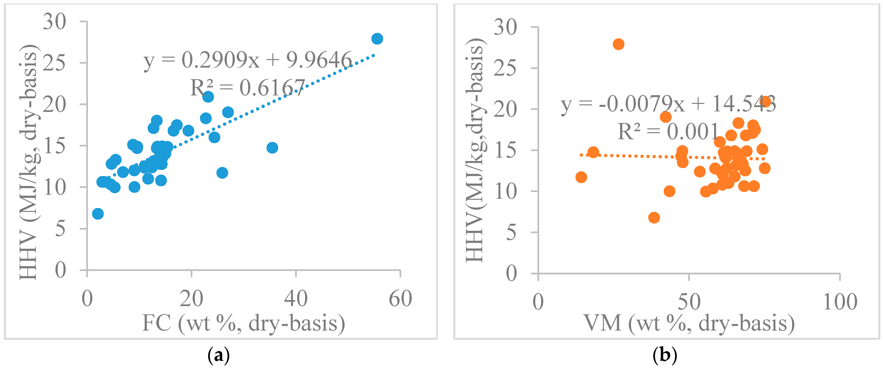
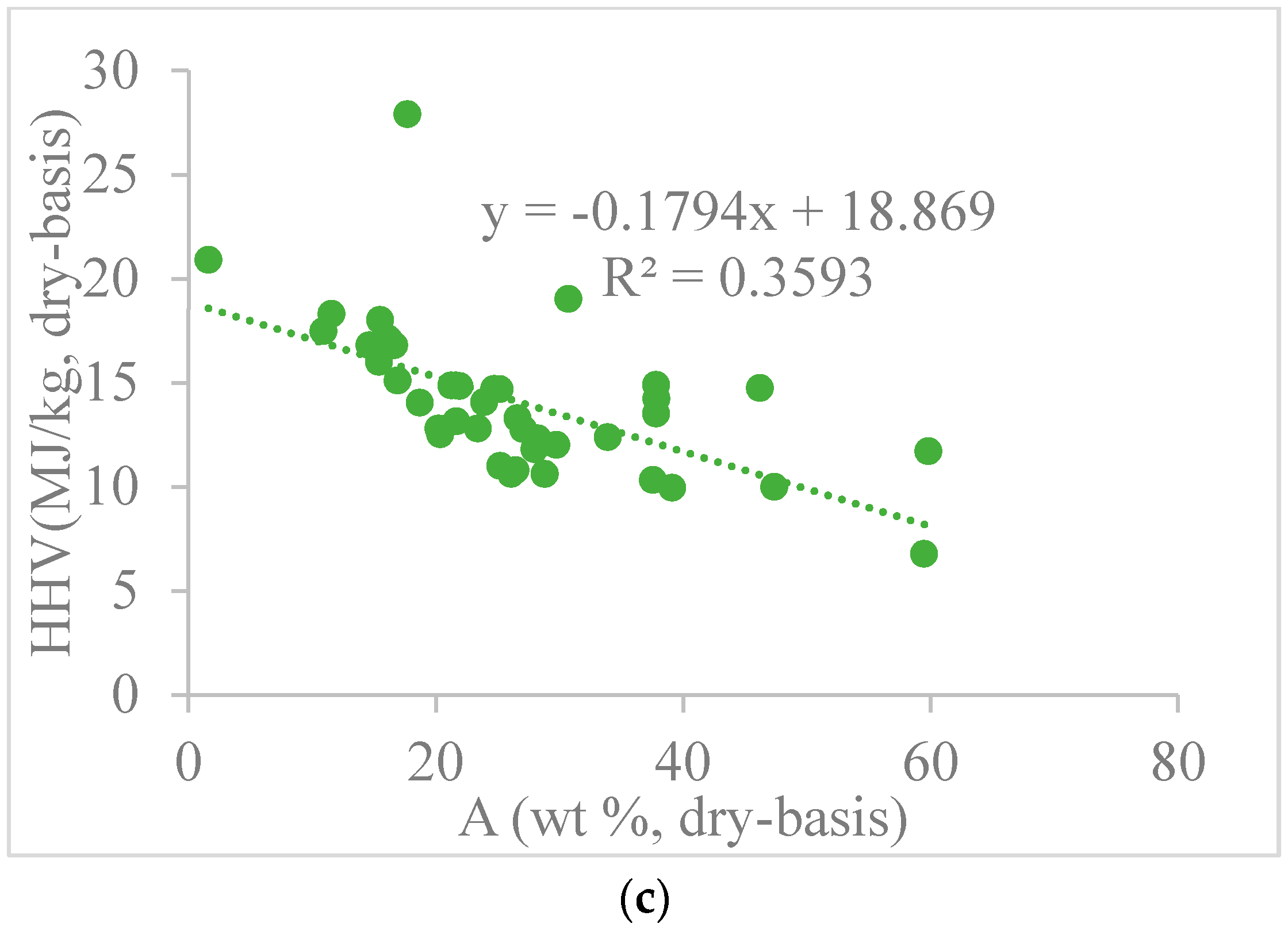
3.1. Effects of Proximate Analysis Composition on HHV

As shown in Figure 1, the HHV of PW samples are plotted as a function of FC, VM, and ash components (in wt %, dry-basis) by using scatter plots to show how HHV results vary with different composition of proximate analysis data. For the instance of PW samples, HHV results were found to increase with the FC contents. In contrast, there is a clear trend in HHV results decreasing with the increase of ash contents. Previous studies have drawn similar conclusions in that FC content has a positive effect whereas ash content has a negative effect on the HHV of raw biomass materials and torreffied biomass materials [28]. For the case of coal, Majumder et al. [14] also found the same trend. This may be possible due to ash having an inert effect on the heating value. Some detrimental effect on the apparent heat obtained during the biomass combustion process because the energy of ash forming inorganics for thermal breakdown and phase transition is taken from biomass combustion process [15]. These results further confirm that ash content is one of the most important fuel properties directly affecting the HHV, with high amounts may making PW less desirable as energy resource during the conversion processes. But the effect of VM composition on the HHV of PW is less obvious. Previous studies also found that the effect of VM content on HHV is much more complicated and inconclusive. High VM does not guarantee a high calorific value since some of the ingredients in VM are formed from non-combustible gases, such as CO2 and H2O [15,27]. Therefore, the results infer that linear regression models for VM may not represent the most appropriate solution to accurately estimate the HHV of PW samples. As such, the polynomial terms, such as quadratic, cubic, and interaction effect are proposed in this study to predict the precise HHV of PW samples.
Correlation is evaluated to measure the strength of the association between the factors (e.g., FC, VM, ash) and response variables (e.g., HHV). As shown in Figure 1, there is a relatively strong linear correlation between the HHV and FC (R2 = 0.6167) while only a moderate correlation exists between the HHV and ash (R2 = 0.3593) with the current PW database. However, Sheng and Azevedo [6] found a different phenomenon for biomass, in that there exists a significant correlation between HHV and ash (R2 = 0.625) while only a trend exists between the HHV and VM (R2 = 0.307). In addition, Akkaya et al. [55] observed a linear relationship between the HHV and two components (VM and FC), as well as a stronger non-linear dependence for percentages of other two components (M and ash) with coal samples. Compared with biomass and coal samples, the correlation between proximate analysis components and HHV for PW samples is significantly different. This suggests that the existing correlation of proximate-based models for solid fuels, such as biomass and coal, are not appropriate for estimating the HHV of PW samples. Thus, fifteen new regression models are proposed to correlate the HHV and proximate analysis components of PW samples.

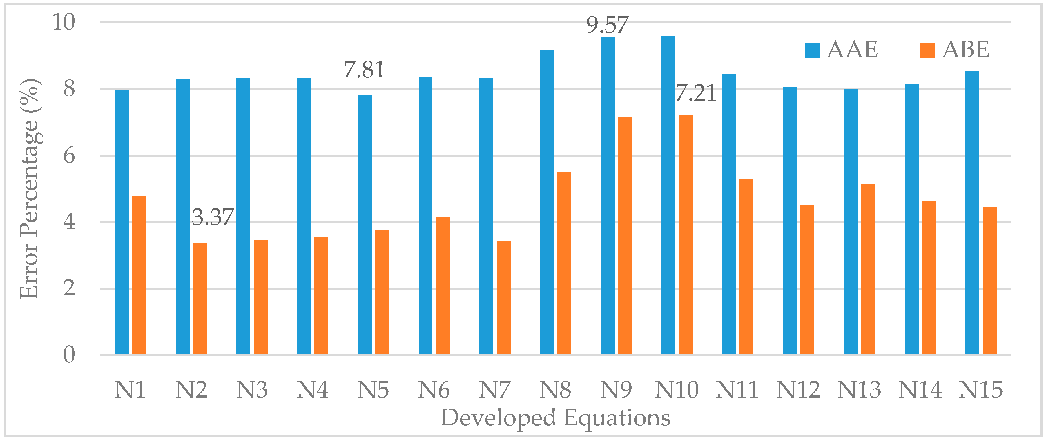
3.2. Derivation of the New Regression Models

As shown in Table 4, fifteen new regression models are developed by using proximate analysis data of thirty-seven PW samples. R2 value, adjusted R2 value, along with AAE and ABE, are also calculated and summarized. Results indicate that new proximate-based regression models can predict the HHV of PW with R2 values ranging between 78.14% and 91.62%. The estimation errors are found to be in the range of 5.98% to 10.36% for AAE, and −0.35% to 1.53% for ABE. In the following section, letter “N” indicates the new regression models derived from this study and “E” indicates the existing models that were developed by other researchers. For instance, N1 indicates the new regression model 1. Excluding N9 and N10, the rest of the new regression models have better R2 values (>0.85) than the previous models. One possible reason for relatively high R2 value is that only one subclass of fuel (PW samples) is being used. Sheng and Azevedo [6] had a similar explanation for why their R2 value was very low (<0.85). They postulated that the low value was due to evaluating a wide range of biomass species that compromised the accuracy of estimation [6]. This infers that considering only PW samples could improve the accuracy of HHV prediction.
According to previous studies, Cordero et al. [11] identified a simple equation based on proximate analysis (VM and FC) that could predict the HHV of lignocellulosic materials as well as char coals. Yin [7] also found that a simple empirical equation based on proximate analysis (VM and FC) is sufficient for estimating the HHV of biomass. However, consideration of only two components (VM and FC) of proximate analysis in N2 has lower R2 value and higher estimation errors than N1, where all three proximate analysis components are included for PW samples. This indicates that a proximate-based regression model in HHV predictions of PW samples should consider FC, VM and ash content. Parikh et al. [20] and Nhuchhen [8] used a similar approach and concluded that developed models with all three components of proximate analysis are required to lower estimation errors. AAE in N1 to N8 is also observed to be lower than AAE in N9 and N10 (about 3%). Since both FC and ash content are applied as quadratic in both N9 and N10, while at least one linear correlation (either FC or ash) are included in models N1 to N8, we can conclude that the multiple linear regression model of all three components of proximate analysis (N1) is the most accurate regression model among N1 to N10.
In further refining the steps (derivation of N11), polynomial relationships (quadratic and cubic) with VM are added to the simple multiple linear regression model (N1) because the observation from Figure 1b identified as the linear model for VM may not represent the most appropriate solution to accurately estimating the HHV of PW samples. This addition shows a further increment of R2 and a reduction of estimation errors. In addition, N12, N13 and N14 are proposed to compare the interaction effect between two proximate components. Even though the interaction effect provides a small contribution in reducing the estimation errors, a significant interaction effect of FC and ash has been identified. Therefore, N15 is developed by combining the simple multiple linear regression model (N1), the polynomial terms of VM (quadratic, cubic), and the best interaction effect (FC and ash). The best-fit regression model (N15) has the highest R2 in 91.62%, lowest AAE in 5.98%, and the lowest ABE in −0.35%. This suggests that consideration of a polynomial dependence of VM as well as interaction effects of FC and ash can improve the accuracy of predicting the HHV of PW samples.

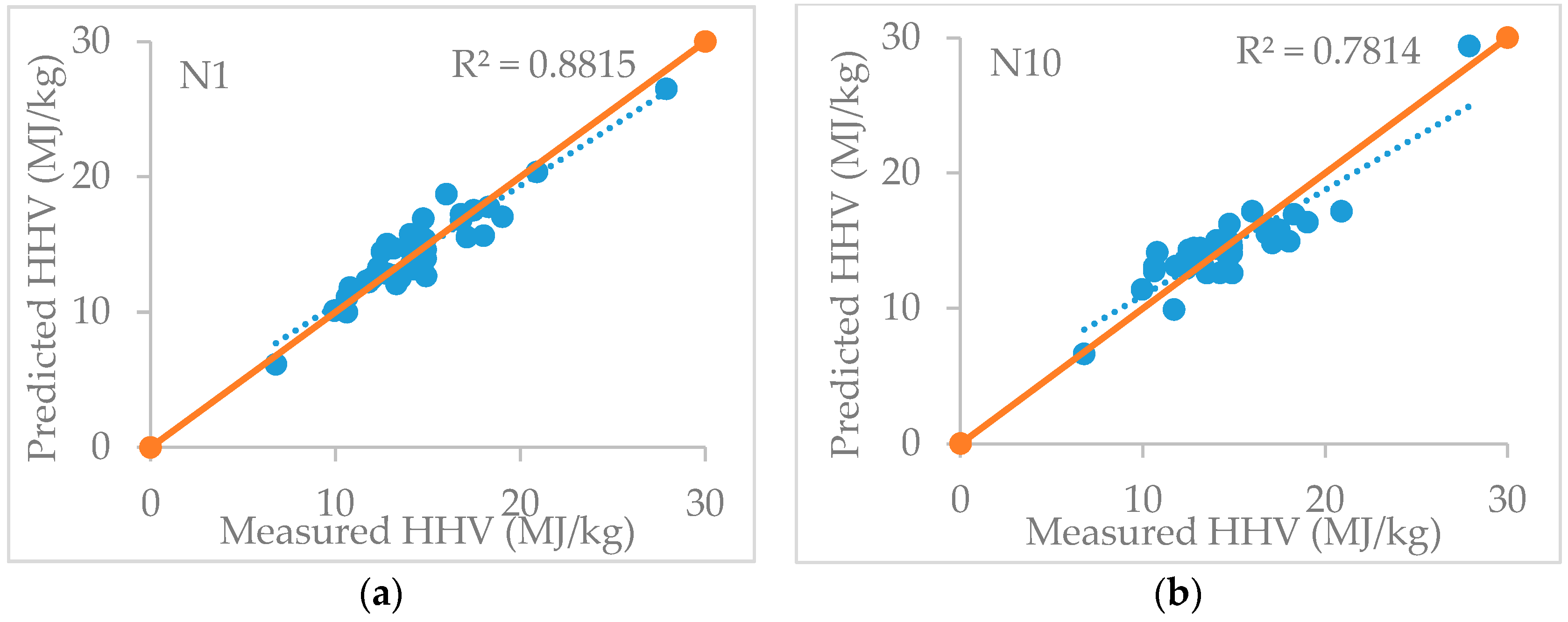
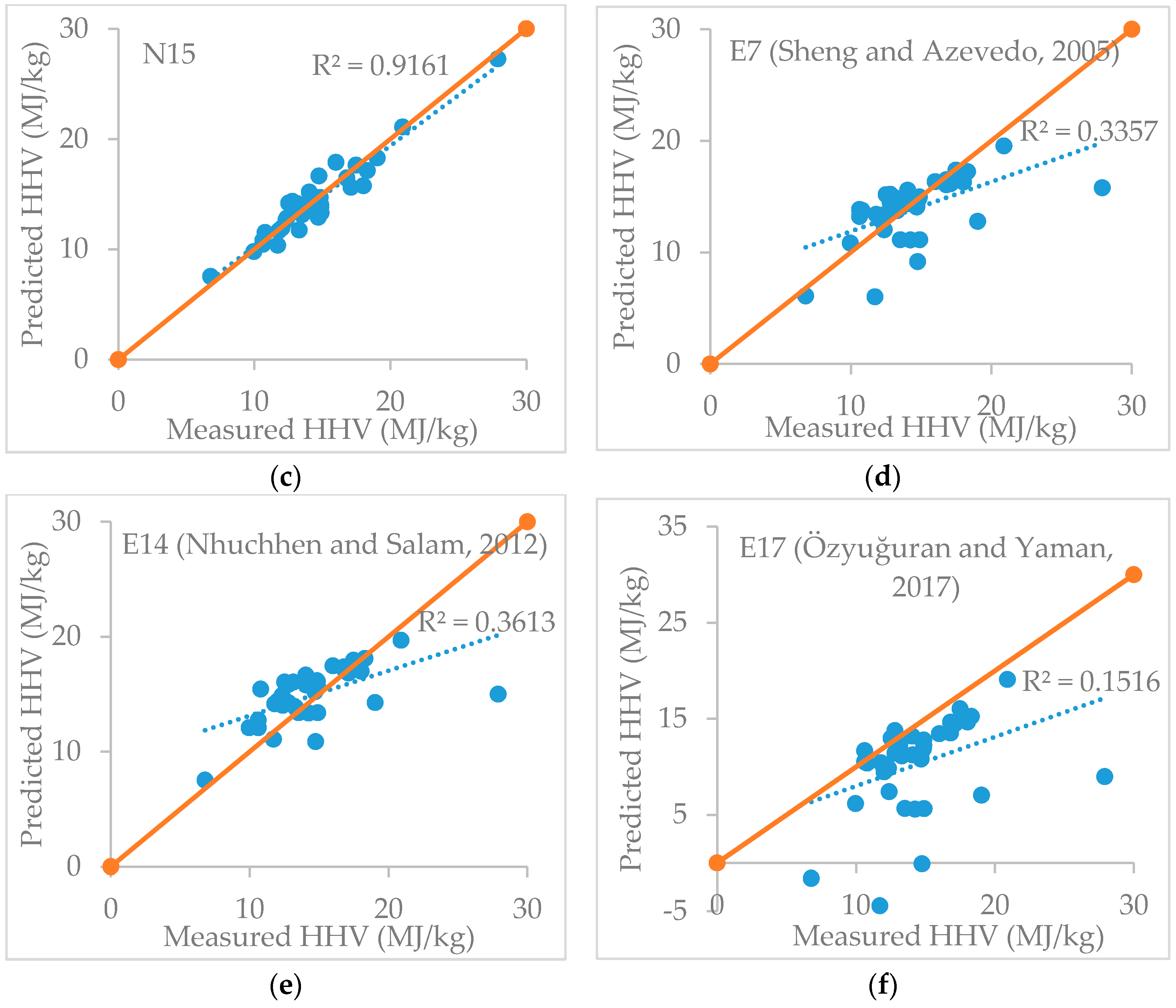
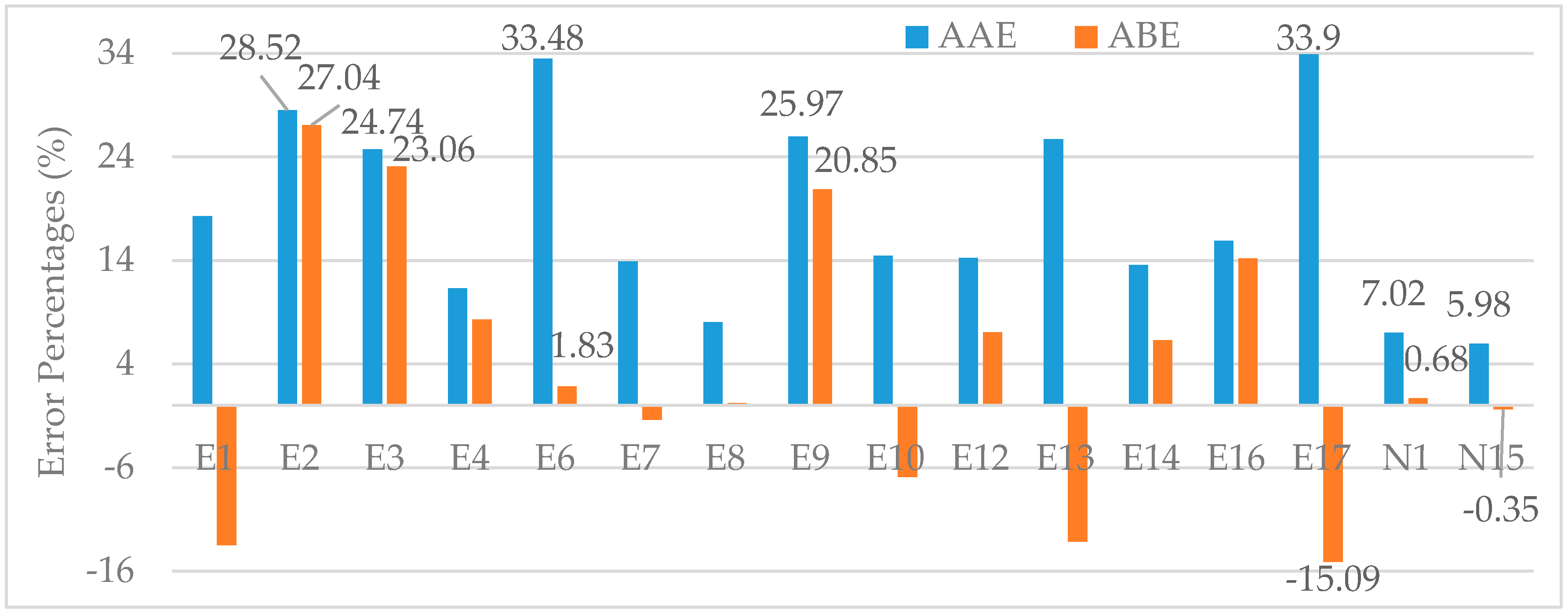
3.3. Validation and Comparative Studies

As shown in Figure 2, the comparison between experimental and predicted HHV results from new regression models (N1, N10 and N15) as well as three existing proximate-based models (E7, E14 and E17) are plotted by using the sample data points from Table 2 (Sample #1–37).
Figure 2d–f indicate that the predicted HHV from existing proximate-based models are far away from the line of HHVpredicted = HHVexperimental (orange lines in Figure 2) and therefore not applicable in predicting the HHV of PW samples. On the other hand, the results show most of the estimated HHV results from new regression models (N1, N10 and N15) are close to the line of HHVpredicted = HHVexperimental, indicating good accuracy for HHV predictions of PW samples. The results further confirm that the new regression models have better accuracy than existing proximate-based models in predicting the HHV of PW samples. It is especially apparent that the predicated points from the best-fit regression model (N15) are close to the measured values while slightly over-predicting or under-predicting the HHV at different points in the curve.
The validations are carried out for the 15 new regression models to ensure the compatibility with other PW samples with different characteristics. As shown in Figure 3, the AAE and ABE of 15 new regression models are calculated by using additional six samples (#38–42, #49) and presented by the bar chart. Results indicate new regression models have an AAE of 7.81 to 9.57% and ABE of 3.37 to 7.21%. Relatively low AAE and ABE infer that new regression models can be used to estimate the HHV of PW samples from proximate analysis data with high accuracy.
Detailed ABE and AAE results of new regression models (N1, N15) and existing proximate-based models (E1 to E17) are calculated using the same data points (#1–37) from Table 2. The results are presented in Figure 4. Overall, the results indicate that the new regression models have lower estimation errors than existing proximate-based models. It is not surprising that the resulting estimation errors from existing proximate-based are very different because the coefficients of the formula and constituent of proximate analysis are considerably different for each case. Three existing proximate-based models, E5, E11 and E15, are excluded due to extremely large estimation errors compared to the other models. AAE of existing models, E2 (coal), E3 (biomass) and E17 (biomass) is overestimated compared to the measured HHV (AAE > 20%) because they were developed for coal and biomass samples. Raw materials of biomass and coal were selected from a wide range of species and are expected to cause large variations. In addition, the existing proximate-based model for subclass of fuels, E6 (municipal solid waste) and E9 (sewage sludge), also have larger AAE values (>25%) due to existing proximate-based models for one specific subclass fuel (e.g., municipal solid waste, sewage sludge) that are not appropriate for the other subclass of fuel (e.g., PW). However, relatively low AAE and ABE prove that the new regression models can generally have higher accuracy than the existing proximate-based models in HHV predictions of PW samples. Among the 15 new regression models, the simple multiple linear regression model (N1) has a R2 value of 88.15% for predicting HHV of PW samples. The best-fit regression model (N15) has the lowest AAE at 5.98% and provides a marginal lower estimation at just 0.35%, further validating the model’s capability in predicting the HHV of PW samples.

4. Conclusions

The HHV (or the energy content) of PW samples is an important attribute when using PW as an energy resource for various thermal conversion processes. In this study, a simple multiple linear regression model and a best -fit regression model are developed to predict HHV of PW samples from proximate analysis data. Results show that the simple multiple linear regression model (N1) can compromise all three components of proximate analysis. Results also show that the polynomial terms for VM, as well as interaction effects of FC and ash, are necessary for the best-fit regression model (N15) to further lower estimation errors. The estimated HHV using the new regression models are closer to experimental results. In addition, these new regression models provide better prediction power than the existing proximate-based models (E1 to E17) when predicting the HHV from proximate data for PW samples. Therefore, these new regression models can be used to predict the HHV of PW samples from proximate analysis data, where sophisticated equipment for experimental determination of the HHV are not available. In future study, additional PW samples will be collected from poultry farms to study effect of proximate analysis compositions on the HHV. In addition, more powerful tools (e.g., data mining, neural networks, machine learning) will be adopted to reduce errors and provide much more robust results.

Supplementary Materials

The following are available online at https://www.mdpi.com/2079-9276/7/3/39/s1. Table S1: Proximate analyses, ultimate analyses, and HHV of poultry waste samples.

Author Contributions

X.Q. reviewed published literature reviews and collected properties data of poultry waste samples. X.Q. and S.L. conceived and designed approach to construct the regression models. X.Q. analyzed data points and developed new regression models which presented in this study. X.Q. and S.L. wrote the draft manuscript. A.-m.S., G.C. and S.L. reviewed this manuscript and provided their constructive comments and suggestions to improve the quality of article.

Acknowledgments

The authors received funds from Graduate Student Association at Morgan State University for covering the costs to publish in open access. The author (Xuejun Qian) would like to acknowledge the Graduate Student Association, School of Graduate Studies at Morgan State University and The Abell Foundation for providing a partial financial support for this study. In addition, author (Xuejun Qian) would like to appreciate kind support of research facilities from Center for Advanced Energy Systems and Environmental Control Technologies (CAESECT).

Conflicts of Interest

The authors declare no conflict of interest.

References

  1. Lynch, D.; Henihan, A.M.; Bowen, B.; Lynch, D.; McDonnell, K.; Kwapinski, W.; Leahy, J.J. Utilisation of poultry litter as an energy feedstock. Biomass Bioenergy 2013, 49, 197–204. [Google Scholar] [CrossRef] [Green Version]
  2. Kelleher, B.P.; Leahy, J.J.; Henihan, A.M.; O’dwyer, T.F.; Sutton, D.; Leahy, M.J. Advances in poultry litter disposal technology—A review. Bioresour. Technol. 2002, 83, 27–36. [Google Scholar] [CrossRef]
  3. Abelha, P.; Gulyurtlu, I.; Boavida, D.; Barros, J.S.; Cabrita, I.; Leahy, J.; Kelleher, B.; Leahy, M. Combustion of poultry litter in a fluidised bed combustor. Fuel 2003, 82, 687–692. [Google Scholar] [CrossRef]
  4. Li, S.; Wu, A.; Deng, S.; Pan, W.P. Effect of co-combustion of chicken litter and coal on emissions in a laboratory-scale fluidized bed combustor. Fuel Process. Technol. 2008, 89, 7–12. [Google Scholar] [CrossRef]
  5. Dalólio, F.S.; da Silva, J.N.; de Oliveira, A.C.C.; Tinôco, I.D.F.F.; Barbosa, R.C.; de Oliveira Resende, M.; Albino, L.F.T.; Coelho, S.T. Poultry litter as biomass energy: A review and future perspectives. Renew. Sustain. Energy Rev. 2017, 76, 941–949. [Google Scholar] [CrossRef]
  6. Sheng, C.; Azevedo, J.L.T. Estimating the higher heating value of biomass fuels from basic analysis data. Biomass Bioenergy 2005, 28, 499–507. [Google Scholar] [CrossRef]
  7. Yin, C.Y. Prediction of higher heating values of biomass from proximate and ultimate analyses. Fuel 2011, 90, 1128–1132. [Google Scholar] [CrossRef] [Green Version]
  8. Nhuchhen, D.R.; Salam, P.A. Estimation of higher heating value of biomass from proximate analysis: A new approach. Fuel 2012, 99, 55–63. [Google Scholar] [CrossRef]
  9. Ghugare, S.B.; Tiwary, S.; Elangovan, V.; Tambe, S.S. Prediction of higher heating value of solid biomass fuels using artificial intelligence formalisms. Bioenergy Res. 2014, 7, 681–692. [Google Scholar] [CrossRef]
  10. Vargas-Moreno, J.M.; Callejón-Ferre, A.J.; Pérez-Alonso, J.; Velázquez-Martí, B. A review of the mathematical models for predicting the heating value of biomass materials. Renew. Sustain. Energy Rev. 2012, 16, 3065–3083. [Google Scholar] [CrossRef]
  11. Cordero, T.; Marquez, F.; Rodriguez-Mirasol, J.; Rodriguez, J.J. Predicting heating values of lignocellulosics and carbonaceous materials from proximate analysis. Fuel 2001, 80, 1567–1571. [Google Scholar] [CrossRef]
  12. Quiroga, G.; Castrillón, L.; Fernández-Nava, Y.; Marañón, E. Physico-chemical analysis and calorific values of poultry manure. Waste Manag. 2010, 30, 880–884. [Google Scholar] [CrossRef] [PubMed]
  13. Cotana, F.; Coccia, V.; Petrozzi, A.; Cavalaglio, G.; Gelosia, M.; Merico, M.C. Energy valorization of poultry manure in a thermal power plant: Experimental campaign. Energy Procedia 2014, 45, 315–322. [Google Scholar] [CrossRef]
  14. Majumder, A.K.; Jain, R.; Banerjee, P.; Barnwal, J.P. Development of a new proximate analysis based correlation to predict calorific value of coal. Fuel 2008, 87, 3077–3081. [Google Scholar] [CrossRef]
  15. Özyuğuran, A.; Yaman, S. Prediction of Calorific Value of Biomass from Proximate Analysis. Energy Procedia 2017, 107, 130–136. [Google Scholar] [CrossRef]
  16. Huang, C.; Han, L.; Liu, X.; Yang, Z. Models predicting calorific value of straw from the ash content. Int. J. Green Energy 2008, 5, 533–539. [Google Scholar] [CrossRef]
  17. Küçükbayrak, S.; Dürüs, B.; Meríçboyu, A.E.; Kadioġlu, E. Estimation of calorific values of Turkish lignites. Fuel 1991, 70, 979–981. [Google Scholar] [CrossRef]
  18. Basu, P. Biomass Gasification and Pyrolysis: Practical Design and Theory, 1st ed.; Elsevier: Oxford, UK, 2010; ISBN 9780123749888. [Google Scholar]
  19. Demirbas, A. Prediction of higher heating values for vegetable oils and animal fats from proximate analysis data. Energy Source Part A 2009, 31, 1264–1270. [Google Scholar] [CrossRef]
  20. Parikh, J.; Channiwala, S.A.; Ghosal, G.K. A correlation for calculating HHV from proximate analysis of solid fuels. Fuel 2005, 84, 487–494. [Google Scholar] [CrossRef]
  21. Jiménez, L.; González, F. Study of the physical and chemical properties of lignocellulosic residues with a view to the production of fuels. Fuel 1991, 70, 947–950. [Google Scholar] [CrossRef]
  22. Demirbaş, A. Calculation of higher heating values of biomass fuels. Fuel 1997, 76, 431–434. [Google Scholar] [CrossRef]
  23. Demirbaş, A. Relationships between heating value and lignin, fixed carbon, and volatile material contents of shells from biomass products. Energy Source 2003, 25, 629–635. [Google Scholar] [CrossRef]
  24. Kathiravale, S.; Yunus, M.N.M.; Sopian, K.; Samsuddin, A.H.; Rahman, R.A. Modeling the heating value of Municipal Solid Waste. Fuel 2003, 82, 1119–1125. [Google Scholar] [CrossRef]
  25. Thipkhunthod, P.; Meeyoo, V.; Rangsunvigit, P.; Kitiyanan, B.; Siemanond, K.; Rirksomboon, T. Predicting the heating value of sewage sludges in Thailand from proximate and ultimate analyses. Fuel 2005, 84, 849–857. [Google Scholar] [CrossRef]
  26. Callejón-Ferre, A.J.; Velázquez-Martí, B.; López-Martínez, J.A.; Manzano-Agugliaro, F. Greenhouse crop residues: Energy potential and models for the prediction of their higher heating value. Renew. Sustain. Energy Rev. 2011, 15, 948–955. [Google Scholar] [CrossRef]
  27. García, R.; Pizarro, C.; Lavín, A.G.; Bueno, J.L. Spanish biofuels heating value estimation. Part II: Proximate analysis data. Fuel 2014, 117, 1139–1147. [Google Scholar] [CrossRef]
  28. Nhuchhen, D.R.; Afzal, M.T. HHV Predicting Correlations for Torrefied Biomass Using Proximate and Ultimate Analyses. Bioengineering 2017, 4, 7. [Google Scholar] [CrossRef] [PubMed]
  29. Whitely, N.; Ozao, R.; Artiaga, R.; Cao, Y.; Pan, W.P. Multi-utilization of chicken litter as biomass source. Part I. Combustion. Energy Fuel 2006, 20, 2660–2665. [Google Scholar] [CrossRef]
  30. Topal, H.; Amirabedin, E. Determination of some important emissions of poultry waste co-combustion. Sci. J. Riga Tech. Univ. Environ. Clim. Technol. 2012, 8, 12–17. [Google Scholar] [CrossRef] [Green Version]
  31. Reardon, J.P.; Lilley, A.; Wimberly, J.; Browne, K.; Beard, K.; Avens, J. Demonstration of a Small Modular Biopower System Using Poultry Litter; DOE SBIR Phase-I Final Report; Community Power Corporation: Englewood, CO, USA, 2001. Available online: https://www.osti.gov/servlets/purl/794292/ (accessed on 2 May 2018).
  32. Bock, B.R. Poultry litter to energy: Technical and economic feasibility. Available online: brbock.com/RefFiles/PoultryLitter_Energy.doc (accessed on 2 May 2018).
  33. Henihan, A.M.; Leahy, M.J.; Leahy, J.J.; Cummins, E.; Kelleher, B.P. Emissions modeling of fluidised bed co-combustion of poultry litter and peat. Bioresour. Technol. 2003, 87, 289–294. [Google Scholar] [CrossRef] [Green Version]
  34. Ghanim, B.M.; Kwapinski, W.; Leahy, J.J. Hydrothermal carbonisation of poultry litter: Effects of initial pH on yields and chemical properties of hydrochars. Bioresour. Technol. 2017, 238, 78–85. [Google Scholar] [CrossRef] [PubMed]
  35. Patel, B.; McQuigg, K.; Toerne, R. Integration of poultry Litter Gasification with Conventional Pulverized Coal Fired Power Plant. Available online: http://infohouse.p2ric.org/ref/35/34198.pdf (accessed on 2 May 2018).
  36. Ekpo, U.; Ross, A.B.; Camargo-Valero, M.A.; Williams, P.T. A comparison of product yields and inorganic content in process streams following thermal hydrolysis and hydrothermal processing of microalgae, manure and digestate. Bioresour. Technol. 2016, 200, 951–960. [Google Scholar] [CrossRef] [PubMed] [Green Version]
  37. Kantarli, I.C.; Kabadayi, A.; Ucar, S.; Yanik, J. Conversion of poultry wastes into energy feedstocks. Waste Manag. 2016, 56, 530–539. [Google Scholar] [CrossRef] [PubMed]
  38. Florin, N.H.; Maddocks, A.R.; Wood, S.; Harris, A.T. High-temperature thermal destruction of poultry derived wastes for energy recovery in Australia. Waste Manag. 2009, 29, 1399–1408. [Google Scholar] [CrossRef] [PubMed]
  39. Priyadarsan, S.; Annamalai, K.; Sweeten, J.M.; Holtzapple, M.T.; Mukhtar, S. Co-gasification of blended coal with feedlot and chicken litter biomass. Proc. Combust. Inst. 2005, 30, 2973–2980. [Google Scholar] [CrossRef]
  40. Miller, S.F.; Miller, B.G. The occurrence of inorganic elements in various biofuels and its effect on ash chemistry and behavior and use in combustion products. Fuel Process. Technol. 2007, 88, 1155–1164. [Google Scholar] [CrossRef]
  41. Cantrell, K.B.; Hunt, P.G.; Uchimiya, M.; Novak, J.M.; Ro, K.S. Impact of pyrolysis temperature and manure source on physicochemical characteristics of biochar. Bioresour. Technol. 2012, 107, 419–428. [Google Scholar] [CrossRef] [PubMed]
  42. Striūgas, N.; Zakarauskas, K.; Džiugys, A.; Navakas, R.; Paulauskas, R. An evaluation of performance of automatically operated multi-fuel downdraft gasifier for energy production. Appl. Therm. Eng. 2014, 73, 1151–1159. [Google Scholar] [CrossRef]
  43. Giuntoli, J.; De Jong, W.; Arvelakis, S.; Spliethoff, H.; Verkooijen, A.H.M. Quantitative and kinetic TG-FTIR study of biomass residue pyrolysis: Dry distiller’s grains with solubles (DDGS) and chicken manure. J. Anal. Appl. Pyrolysis 2009, 85, 301–312. [Google Scholar] [CrossRef]
  44. Burra, K.G.; Hussein, M.S.; Amano, R.S.; Gupta, A.K. Syngas evolutionary behavior during chicken manure pyrolysis and air gasification. Appl. Energy 2016, 181, 408–415. [Google Scholar] [CrossRef] [Green Version]
  45. Mehmood, S.; Reddy, B.V.; Rosen, M.A. Energy analysis of a biomass co-firing based pulverized coal power generation system. Sustainability 2012, 4, 462–490. [Google Scholar] [CrossRef]
  46. Leahy, M.J.; Henihan, A.M.; Kelleher, B.P.; Leahy, J.J.; O’Connor, J. Mitigation of Large-Scale Organic Waste Damage Incorporating a Demonstration of a Closed Loop Conversion of Poultry Waste to Energy at the Point of Source, (2000-LS-1-M2) Final Report. 2007. Available online: https://ulir.ul.ie/handle/10344/4053 (accessed on 2 May 2018).
  47. Ghani, W.A.W.A.K. Co-Combustion of Biomass Fuels with Coal in a Fluidised Bed Combustor. Ph.D. Thesis, University of Sheffield, Sheffield, UK, May 2005. [Google Scholar]
  48. Vamvuka, D.; Sfakiotakis, S.; Panopoulos, K. An experimental study on the thermal valorization of municipal and animal wastes. Int. J. Energy Environ. Econ. 2013, 4, 191–198. [Google Scholar]
  49. Taupe, N.; Jeahy, J.J.; Kwapinski, W. Gasification and Pyrolysis of Poultry Litter—An Opportunity to Produce Bioenergy and Nutrient Rich Biochar; Joint Scientific Workshop: Erfurt, Germany, 2015. [Google Scholar]
  50. Jia, L.; Anthony, E.J. Combustion of poultry-derived fuel in a coal-fired pilot-scale circulating fluidized bed combustor. Fuel Process. Technol. 2011, 92, 2138–2144. [Google Scholar] [CrossRef]
  51. Dayananda, B.S.; Sreepathi, L.K. An experimental study on gasification of chicken litter. Int. Res. J. Environ. Sci. 2013, 2, 63–67. [Google Scholar]
  52. Di Gregorio, F.; Santoro, D.; Arena, U. The effect of ash composition on gasification of poultry wastes in a fluidized bed reactor. Waste Manag. Res. 2014, 32, 323–330. [Google Scholar] [CrossRef] [PubMed]
  53. Manure to Energy Feasibility Study for Duncannon Borough. Available online: http://www.gabi-software.com/uploads/media/Manure_to_Energy_Feasibility_Study_03.pdf (accessed on 2 May 2018).
  54. Acharya, B.; Dutta, A.; Mahmud, S.; Tushar, M.; Leon, M. Ash analysis of poultry litter, willow and oats for combustion in boilers. J. Biomass Biofuel 2014, 1, 16–26. [Google Scholar] [CrossRef]
  55. Akkaya, A.V. Proximate analysis based multiple regression models for higher heating value estimation of low rank coals. Fuel Process. Technol. 2009, 90, 165–170. [Google Scholar] [CrossRef]
Figure 1. Relationships between HHV and composition of individual proximate analysis components: (a) Scatter Plot of fixed carbon (FC) along with HHV results; (b) Scatter plot of volatile matter (VM) along with HHV results; (c) Scatter plot of Ash (A) along with HHV results.
Resources 07 00039 g001aResources 07 00039 g001b
Figure 2. Comparison between predicted and experimental HHV results for new regression models and existing proximate-based models: (a) Simple multiple linear regression model (N1); (b) new lowest R2 value regression model (N10); (c) best-fit regression model (N15); (d) Sheng and Azevedo’s model (E7); (e) Nhuchhen and Salam’s model (E14); (f) Özyuğuran and Yaman’s model (E17). The orange lines represent the points where HHVpredicted = HHVexperimental.
Resources 07 00039 g002aResources 07 00039 g002b
Figure 3. Summary of calculated error percentages, including averaged absolute error (AAE) and averaged based error (ABE) of new developed models by using additional PW samples.
Resources 07 00039 g003
Figure 4. Comparison of error percentages (both AAE and ABE) between existing proximate-based models (E1–E17) and new regression models (N1, N15).
Resources 07 00039 g004
Table 1. Proximate analysis-based models for the HHV Prediction from the literature review.
Existing ModelsHHV (MJ/kg) *Raw MaterialsRef.
E1HHV = −10.81408 + 0.3133 (VM + FC)Lignocellulosic Residues[21]
E2HHV = 76.56 − 1.3 (VM + A) + 7.3 × 10⁻³ (VM + A)2Coal[17]
E3HHV = 0.196 (FC) + 14.119Biomass[22]
E4HHV = 0.3543 FC + 0.1708 VMLignocellulosics & Charcoals[11]
E5HHV = −0.066 (FC)2 + 0.5866 (FC) + 8.752Shell of biomass[23]
E6HHV = 0.356047 VM − 0.118035 FC − 5.600613Municipal solid waste[24]
E7HHV = 19.914 − 0.2324 ABiomass fuels[6]
E8HHV = 0.3536 (FC) + 0.1559 (VM) − 0.0078 ASolid fuels[20]
E9HHV = 0.25575 VM + 0.28388 FC − 2.38638Sewage sludge[25]
E10HHV = 18.96016 − 0.22527 AStraw[16]
E11HHV = −0.1882 (VM) + 32.94Vegetable oil and tallow[19]
E12HHV = 0.1905 VM + 0.2521 FCBiomass[7]
E13HHV = −2.057 − 0.092 A + 0.279 VMGreenhouse crop residues[26]
E14HHV = 20.7999 − 0.3214 VM/FC + 0.0051 (VM/FC)2 − 11.2277 A/VM + 4.4953 (A/VM)2 − 0.7223 (A/VM)3 + 0.038 (A/VM)4 + 0.0076 FC/ABiomass[8]
E15HHV = 1.83 × 10⁴ − 3.98 A2 − 112.10 ASpanish biofuels[27]
E16HHV = 0.1846 VM + 0.3525 FCTorrefied biomass[28]
E17HHV = 10.982 + 0.1136 VM − 0.2848 ABiomass[15]
* HHV = Higher Heating Value; FC = Fixed Carbon; VM = Volatile Matter; A = Ash.
Table 2. Summary of FC, VM, and A Content (wt %) along with HHV results (MJ/kg) in dry-basis.
No.FC 1VM 2ASH 3HHV 4Ref.
12.9868.2528.7710.62[3]
26.8865.1627.9611.8[4]
39.0761.229.7312.02[29]
411.0260.7728.2112.33[29]
55.3155.6139.099.96[29]
62.0838.4659.466.78[29]
713.3671.2615.4918.02[1]
814.447.9337.7913.52[1]
914.447.8237.7914.9[1]
1011.0568.6320.3312.52[30]
1112.453.633.912.38[31]
1215.462.721.914.84[31]
131566.318.714.05[31]
1417.271.910.917.48[31]
151462.223.914.07[31]
1613.4965.121.6114.87[32]
172.9168.2828.8110.62[33]
1812.7471.1116.1617.11[34]
1913.3661.4925.1514.69[35]
2022.7766.3911.5418.3[36]
2124.460.215.416[37]
2223.275.31.620.9[38]
2319.4263.9716.6116.8[39]
249.6369.1321.2514.87[40]
252742.330.719.03[41]
2635.518.346.214.75[41]
2716.5668.8314.6116.8[42]
285.567.926.613.3[43]
299.665.724.714.7[43]
3012.865.5621.6513.15[44]
3114.4547.4237.8314.24[45]
3214.1760.9926.4210.79[46]
3313.8862.5523.3912.8[46]
3425.914.359.811.71[20]
353.3771.5426.0910.62[47]
3655.626.717.727.9[48]
374.775.120.212.8[49]
3814.358.6427.0612.77[50]
3911.763.125.211[38]
409.0843.5747.3510[39]
418.874.316.915.11[41]
424.5357.9337.5410.33[51]
43--17.214.59[52]
44--25.113.67[52]
45--22.915.28[53]
46-26.5610.614.587[13]
47-64.4315.4111.552[13]
483.354.3-10.1[54]
4911.9863.9624.0614.34
1 FC = Fixed Carbon; 2 VM = Volatile Matter; 3 A = Ash; 4 HHV = Higher Heating Value.
Table 3. List of proposed regression models to predict the HHV of PW samples.
No.Proposed New Models *Note
1HHV = a + bFC + cVM + dALinear (FC, VM, A)
2HHV = a + bFC + cVMLinear (FC, VM)
3HHV = a + bFC + cASHLinear (FC, A)
4HHV = a + bVM + cASHLinear (VM, A)
5HHV = a + bFC2 + cVM + dAQuadratic (FC), Linear (VM, A)
6HHV = a + bFC + cVM2 + dAQuadratic (VM), Linear (FC, A)
7HHV = a + bFC + cVM + dA2Quadratic (A), Linear (FC, VM)
8HHV = a + bFC2 + cVM2 + dAQuadratic (FC, VM), Linear (A)
9HHV = a + bFC2 + cVM + dA2Quadratic (FC, A), Linear (VM)
10HHV = a + bFC2 + cVM2 + dA2Quadratic (FC, VM, A)
11HHV = a + bFC + cVM + dA + eVM2 + fVM3Linear (FC, VM, A), Quadratic & Cubic (VM)
12HHV = a + bFC + cVM + dA + eFC × VMLinear (FC, VM, A), Interaction (FC&VM)
13HHV = a + bFC + cVM + dA + eFC × ALinear (FC, VM, A), Interaction (FC&A)
14HHV = a + bFC + cVM + dA + eVM × ALinear (FC, VM, A), Interaction (VM&A)
15HHV = a + bFC + cVM + dA + eVM2 + fVM3 + gFC × ALinear (FC, VM, A), Quadratic & Cubic (VM), Interaction (FC&A)
* HHV = Higher Heating Value; FC = Fixed Carbon; VM = Volatile Matter; A = Ash; a, b, c, d, e, f and g are the constant terms for the proposed regression models.
Table 4. Summary of new regression models for PW samples.
No.Developed New Regression Model *Percentage (%)
R2R2(adj)AAEABE
N1HHV = 174.3 − 1.335 FC − 1.596 VM − 1.749 A88.1587.087.020.68
N2HHV = −0.33 + 0.4109 FC + 0.1461 VM85.7284.887.500.70
N3HHV = 14.355 + 0.2642 FC − 0.1480 A86.1185.297.420.69
N4HHV = 40.89 − 0.2651 VM − 0.4138 A86.7385.957.250.61
N5HHV = 36.27 + 0.00104 FC2 − 0.2140 VM − 0.3651 A87.0385.857.230.75
N6HHV = 20.60 + 0.1900 FC − 0.000823 VM2 − 0.2281 A86.4385.207.280.66
N7HHV = −0.02 + 0.4077 FC + 0.1426 VM − 0.00006 A285.7284.427.530.73
N8HHV = 28.46 + 0.002104 FC2 − 0.001712 VM2 − 0.3205 A86.3885.147.730.90
N9HHV = 18.16 + 0.00425 FC2 − 0.0463 VM − 0.00288 A278.3776.4010.361.47
N10HHV = 15.41 + 0.004800 FC2 − 0.000145 VM2 − 0.002430 A278.1476.1510.311.53
N11HHV = 143.7 − 1.161 FC − 0.364 VM − 1.562 A − 0.02458 VM2 + 0.000173 VM391.5490.186.050.47
N12HHV = 174.3 − 1.331 FC − 1.595 VM − 1.751 A − 0.00012 FC × VM88.1686.687.010.46
N13HHV = 172.2 − 1.262 FC − 1.587 VM − 1.698 A − 0.00237 FC × A88.9187.536.740.57
N14HHV = 175.2 − 1.332 FC − 1.615 VM − 1.780 A + 0.000652 VM × A88.3286.867.050.20
N15HHV = 140.2 − 1.167 FC − 0.210 VM − 1.558 A − 0.02739 VM2 + 0.000191 VM3 + 0.00104 FC × A91.6289.945.98−0.35
* HHV = Higher Heating Value; FC = Fixed Carbon; VM = Volatile Matter.

