Article

An Approach to the Integrated Design of PCM-Air Heat Exchangers Based on Numerical Simulation: A Solar Cooling Case Study

Thermal Engineering and Energy Systems Group, Aragón Institute for Engineering Research (I3A), University of Zaragoza, Zaragoza 50018, Spain
*
Author to whom correspondence should be addressed.
Resources 2015, 4(4), 796-818; https://doi.org/10.3390/resources4040796
Submission received: 5 June 2015 / Revised: 20 October 2015 / Accepted: 23 October 2015 / Published: 29 October 2015
(This article belongs to the Special Issue Alternative Energy Sources in Developing and Developed Regions)

Abstract

:
A novel technique of design of experiments applied to numerical simulations is proposed in this paper as a methodology for the sizing and design of thermal storage equipment integrated in any specific application. The technique is carried out through the response surfaces in order to limit the number of simulation runs required to achieve an appropriate solution. Thus, there are significant savings on the time spent on the design as well as a potential cost saving on the experimentation if similarity relationships between the prototype and the model are met. The technique is applied here to a previously developed and validated numerical model that simulates the thermal behavior of a phase change material-air heat exchanger. The incorporation of the thermal energy storage unit is analyzed in the case of a solar cooling application, improving the system coefficient of performance. The economic viability is mainly conditioned by the price of the macroencapsulated phase change material.

1. Introduction

A numerical simulation is not itself a design tool, as it provides the system response to previously-imposed operational and experimental conditions [1]. With this work we propose to use the technique of design of experiments (hereafter DOE (Design of Experiments)) applied to numerical simulations as a methodology for the sizing and design of thermal storage equipment. Moreover, instead of a sequential analysis, it is reasonable to use a mathematical and statistical methodology that indicates how to plan the series of experiments (analogously, simulation runs) on the principle of maximum information with minimum effort. The design of experiments methodology is used in a relatively new way to face the problem of the unit design. This method is carried out through the response surfaces in order to limit the number of simulation runs required to achieve an appropriate solution. Thus, savings are achieved on the time spent on the design [2], as well the potential costs of experiments [3], if similarity relationships between the prototype and the model are met.

1.1. DOE Approach

DOE is a very useful statistical approach used to identify a set of process factors (parameters) that are important to the process itself. It is also useful to determine what parameter levels must be maintained to optimize the response of interest [4]. Among its advantages, DOE provides more information than traditional methods of sequential testing [5]. The reader can easily find more information on general aspects of DOE in the open literature: particularly, a brief and clever summary is given by Gunasegaram et al. [3].
This article is focused on the multi-objective optimization phase, so only on the factors previously identified as most relevant, a more refined search is applied. The main objective of this work is the description of the method to simultaneously optimize a set of responses of a thermal energy storage (hereafter, TES (Thermal Energy Storage)) unit (applied to different situations) in order to identify equipment able to provide the best possible performance. This means that we want to know what values of the chosen factors provide the answers with the desired quality (if the requirement is not reached in the response, how much are we willing to accept as tolerable?). All of these values can be identified by a mathematical model, called the response surface that relates the most relevant factors with the answers. The most appropriate experiments to develop these models are described in the response surface designs such as the central composite design and Doehlert design [6]. Central composite design includes central and axial study points. Central points allow a better analysis in the presence of curvature (interaction between factors) and axial points allow analyzing quadratic effects. Therefore, such designs are appropriate when there is a suspicion of the existence of curvature in the response surface. These methods are used to:
  • Find the settings of the factors (operating conditions) that lead to the best response or the settings that meet the process/operation requirements [7,8,9,10];
  • Identify new operating conditions that lead to a demonstrated improvement of the product/process characteristics over the current conditions [1,11];
  • Model a relationship between the quantitative factors and the response [12,13].

1.2. Numerical Simulations Based On DOE

Due to the feedback between simulations and experimental studies, complementing the performance of physical experiments with numerical simulations is becoming increasingly common in many sectors. Some of these numerical experiments are conducted to select the tools, as well as the optimal process parameters that directly allow the development of products that, to some extent, reduce the cost and/or the time required for the corresponding physical experimentation [14,15]. In other cases, the aim is to obtain a deeper understanding of the effect of varying certain process parameters (sensitivity studies) towards the optimization of the process itself [16].
Del Coz Díaz et al. [2] apply DOE to numerical simulations with the aim of limiting the number of runs, significantly reducing the computational cost, and allowing analysis of each parameter influence on the responses of interest. Whitt [17] indicates that as simulations require a statistical analysis of their results, it is appropriate to consider the perspective of experimental design. However, Salazar and Baena Zapata [18] point out that numerical studies based on the methodology of DOE are scarce in the literature. These authors invite researchers working in the area of statistics (although extensible to any other area) to implement the methodology of design and analysis of experiments to numerical simulation studies as they consider that this type of analysis improves the quality of the findings (these being more convincing), as well as the presentation of the simulation analysis results.
In addition, numerical simulation studies considered under this type of approach allow many factors to be analyzed simultaneously, thus optimizing the time spent on the execution of simulations. Further information on DOE concepts applicable to numerical simulations can be found in the work by Gunasegaram et al. [3] where advantages and limitations are reported by the authors.
The use of DOE by means of a response surface analysis is not so different from other more established optimization approaches, such as calculus methods, search methods, linear and dynamic programming, geometric programming, genetic algorithms, artificial neural networks, fuzzy logic, etc. [19,20,21]. In fact, multi-objective optimization problems are traditionally solved by converting the problem into a single-objective optimization problem via a weighted-sum strategy. Here, DOE is conceived as simply the frame of the study, and it is selected because:
  • The overall frame is the DOE approach which includes the response surface technique for multi-objective optimization purposes. One important point of the response surface is that once an optimal solution is calculated, the optimization plot is obtained. The optimal solution serves as the starting point for this plot and then the settings can be modified interactively to see how different settings affect responses. No additional simulation runs are required to achieve any other design allowing to modify factors and getting new responses.
  • This approach is easier and more intuitive to use for “non-expert” designers and decision-makers. The main idea is to provide a more attractive, though rigorous, tool for designers. Traditional optimization techniques usually require a medium-high level of mathematics. Although not trivial, it is much easier to understand and interpret design criteria, as well as the main parameters that define the analysis (such as the weight and the importance).
  • Numerical simulations are not supposed to suffer from variability; however, it is well known that uncertainties in the model input variables/parameters can lead to completely different results in the simulations. In fact, in the type of systems studied here, this occurs with the uncertainty in the inlet temperature (among others). Although not considered in this article, the DOE approach can deal with such uncertainties.

1.3. Design and Optimization of TES Systems for Solar Cooling

Since the COP (Coefficient of Performance) of absorption chillers is usually low, any contribution which may increase the COP value is important for this type of chiller which has many advantages, mainly its low carbon emissions. Therefore, as an example of interest, to apply the methodology we propose a case study of PCM storage integrated in a solar cooling system.
Various works on TES (PCM) in solar cooling systems can be found in the literature, as well as papers on the design and optimization of solar cooling systems by DOE. However, to the best of the authors’ knowledge, the literature on the design and optimization of PCM-TES systems integrated in a selected application is scarce. In this case, the selected application is solar cooling. Then, a TES unit is designed and integrated in the absorption system as an inlet cooling device. The aim of this integration is to avoid inefficiency of air cooled absorption cycle systems due to high temperatures of ambient air. To the best of our knowledge, the study of integrated PCM-TES and absorption cycles as proposed here has never been addressed in the literature. Furthermore, the design and optimization studies here are based on experimental installation results and commercially-available PCM (thermally characterized in the laboratory: cp(T), h(T), λ(T), ρ(T), rheological properties, thermal cycling, etc.).

2. Methodology

The starting point of the work presented here is the theoretical model developed [5] to numerically simulate the thermal behavior of a TES unit based on PCM-air heat exchange [22,23,24]. A sketch of the TES unit is shown in Figure 1. The equipment consists of a series of macroencapsulated PCM plates arranged as parallel plate-walls, separated by air gaps, all contained in a casing with room enough for a centrifugal fan at the bottom. The air flow is conducted to the unit through the inlet, passes between the PCM plate-walls exchanging heat, and is eventually blown out of the unit.
Figure 1. TES unit schematic view and PCM plate layout detail (air flowing through them).
Resources 04 00796 g001
Once the theoretical model is experimentally validated [22,25] the potential application of interest is selected, and then the corresponding TES unit is designed. As an example of the approach, this paper will study the design and integration of a TES unit in an absorption cycle system for solar cooling.

2.1. Similarity Analysis: Scaling the Model
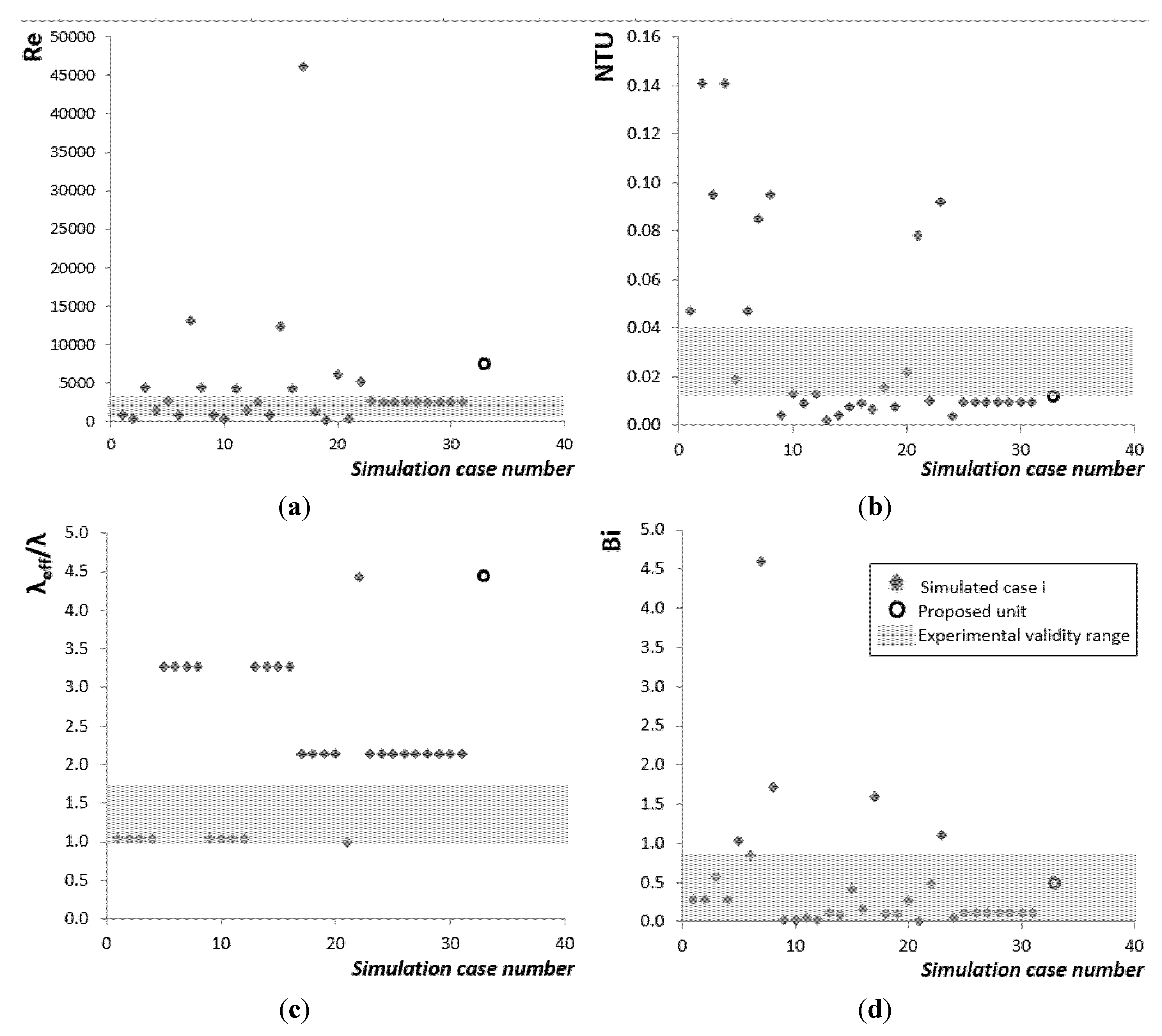
To meet the requirements of the case study, the methodology has been posed for a wider range rather than the experimental validity. Due to the specifications of the solar cooling application, the similarity relationships between the experimental equipment, and the equipment proposed (model-prototype respectively) will not be adjusted in all cases. Thus, calculation of the dimensionless relations of interest that characterize the equipment operation is made for the experimental equipment and for each of the simulated cases. Therefore, the degree of dimensionless similarity of the proposed equipment with the experimental one is checked: within the experimental validity no additional experimentation would be required.

2.2. Validity Range

The experimental validity range has been established for a series of relationships that characterize the heat transfer process in the TES unit. All the validity ranges are shown in Table 1 as well as the temperature ramps used in the experimentation as inlet air condition. Specifically, the ranges of the following relations have been determined:
  • Re is the Reynolds number defined as Re = ρ·v·Dh/µ, where Dh = 4·A/P;
  • NTU is the number of transfer units defined as NTU = (Δx·w)/Cair
  • Bi is the Biot number defined as Bi = h·eencapsulation
  • λeff/λ is the thermal conductivities ratio that quantifies the effect of natural convection within the PCM inside the plate. As this relation goes beyond one, the effect of natural convection is more substantial.
Table 1. Experimental validity ranges.
ReNTUBiλeffRamp (°C/min)
MinMaxMinMaxMinMaxMinMaxMinMax
91725770.0130.0390.0880.8751.001.740.050.25
These parameters are used to ensure that every proposed unit is within the experimental validity range. Their determination is detailed in Dolado [26] (pp. 115–118), and is based on the main Equations (1)–(3) below, where T1 is the air temperature in the TES unit (average between the inlet and the outlet); T2 corresponds to Tmelt; the volumetric expansion coefficient, β, is given by the PCM manufacturer (0.001 K1); the dynamic viscosity value, µ (3.38 × 10³ Pa·s at 40 °C) is provided by the manufacturer and is used as well as those measured in the Malvern laboratory with a Gemini II rheometer; and Nu, Ra, and Pr correspond to the Nusselt, Rayleigh, and Prandtl numbers:
λ e f f = λ · N u L  
N u L = 0.42 R a L 0.25 P r 0.012 ( H / L ) 0.3 , valid for 10  < H / L < 40 ;   10 4 < R a L < 10 7 ;   1 < P r < 2 × 10 4
R a L g · β · ( T 1 T 2 ) · L 3 / ( α · ν )

3. Calculation

Examples of potential uses of such TES units can be found in applications directly related to the ambient air temperature, trying to take advantage of the oscillation in the day/night natural cycle of temperature to facilitate the melting and solidification of the PCM. Here, we will focus on an absorption cycle for solar cooling.

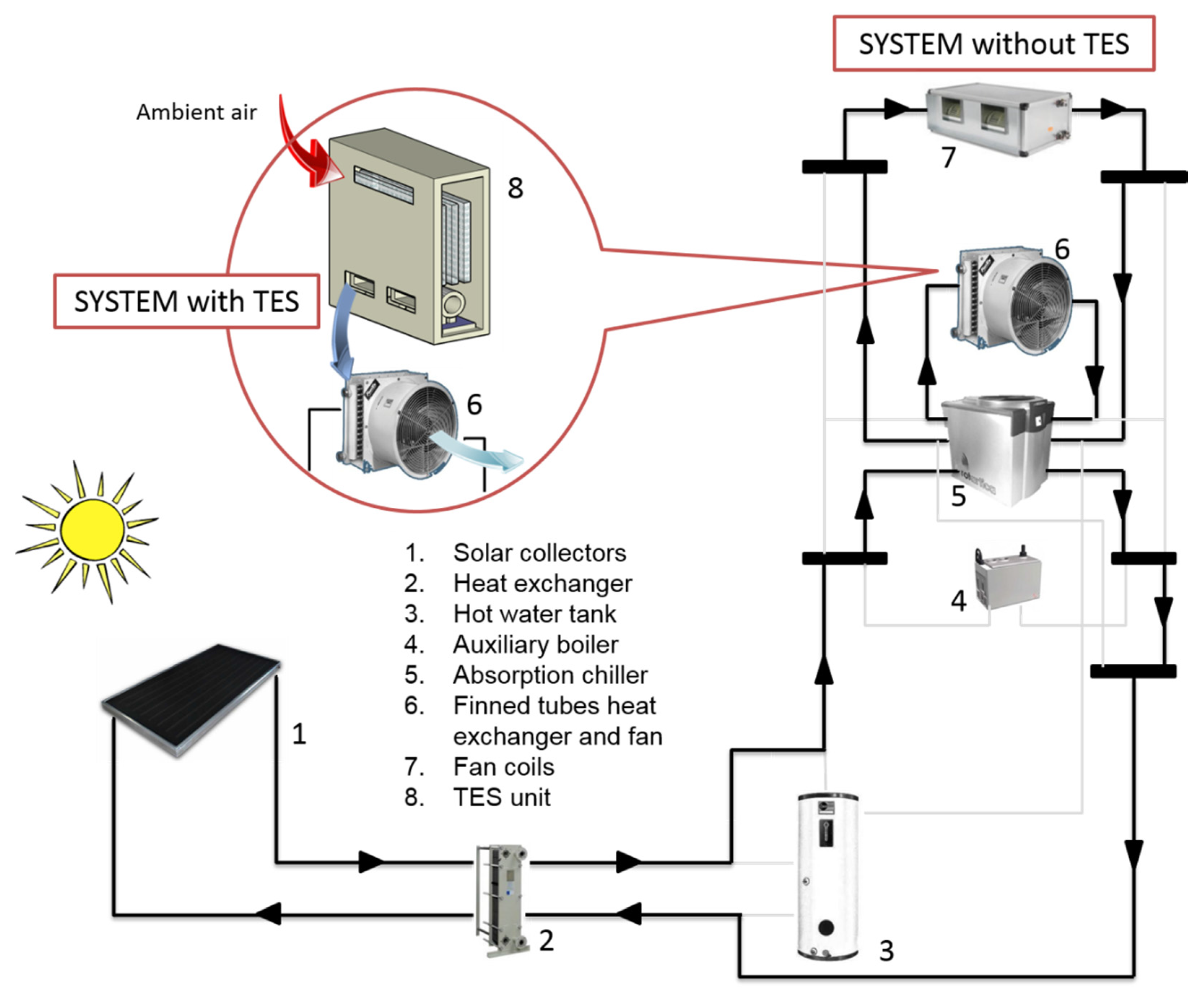
3.1. Potential Application: Case Study of Absorption Cycles for Solar Cooling

In absorption cycles for solar cooling, the behavior of the absorption machine’s internal fluids in the operation process of the cycle is directly dependent on the energy evolution of the fluids outside the machine (water for cooling in the evaporator; water in the cooling tower, or air in the condenser; hot water or steam provided to the hub/generator).
The energy balances applied to all heat exchangers in the machine and the temperature levels of the previous source determine the stability of the cycle: the balance is derived from both kinetic and thermodynamic effects. The machine is constantly adapting to the changing conditions in the external circuits looking for this balance. What if the external conditions cannot be maintained? How does the machine perform? This situation can occur when, for example, on a very hot and humid summer day the cooling tower cannot meet the thermal demand of the required heat dissipation. What is observed is a reduction in the system performance and a dependence of the heat rate and the machine COP on those changing conditions.

3.2. A Real Case of an Absorption Cycle and a Proposed Combi-System with a PCM Storage Unit

An absorption machine manufactured by Rotartica was considered. In particular, operation data of the Rotartica Solar 045v model (air-cooled, LiBr-H2O pair, single effect) are available. The system is installed and is currently working in the sports hall at the University of Zaragoza (Spain). The machine ejects heat from the system through a finned cooling coil and an axial fan that allows blowing outside air to the coil. Hot water is cooled as it transfers heat from the tube walls of the coil to the ambient air. Thus, in the hottest days of the year, if the air temperature is above 35 °C the absorption machine will not work properly [27].
Both the COP and the cooling capacity of the solar cooling system reduce linearly with increasing ambient temperature, as described in [28]. The authors reported an average COP of 0.51 in 2008. The measured average cooling power for this system is 13 kW, and the volumetric air flow required to dissipate the heat in the condenser is about 5500 m3/h. Given these conditions, it is proposed to place the TES unit just before the entrance to the air-condensing unit, which will soften the increase in the ambient air temperature at the condenser inlet. Thus, as the ambient air temperature increases and the TES unit cushions its effect, both the COP and the cooling power of the system will improve compared to the same system without the TES unit.
The coefficient of performance (COP) of the chiller indicates the amount of required heat and electricity per unit of ‘produced’ cold, and it was determined by Monné et al. [28] as follows:
C O P = W ˙ c h / ( W ˙ e W ˙ g )  
where W ˙ e is the electricity consumption of the absorption chiller. W ˙ g is the generator power (heat exchanged from the solar heated water to the LiBr-H2O solution in the generator):
W ˙ g = m ˙ g · c p · ( T g , i T g , o )
where Tg,i and Tg,o are measured at the inlet and outlet entries of the generator, respectively. W ˙ c h is the chilling power (heat exchanged from the chilling circuit to the evaporator):
W ˙ c h = m ˙ c h · c p · ( T e v , i T e v , o )
where Tev,i and Tev,o are measured at the inlet and outlet entries of the evaporator, respectively.
Then, using real operational data of the absorption system, Monné et al. correlated COP with the temperature of the air at the inlet of the absorption machine (i.e., ambient temperature). This correlation is the one used in this paper and was extracted from Figure 5 of [28]:
C O P = 0.0111 · T ( ° C ) + 0.8778  

3.3. Design

The operation outline of the solar cooling system is shown in Figure 2 (further details can be found in Monné et al., 2011 [28]). The TES unit will be placed on the roof of the building to let the ambient air pass through it before heading to the condenser unit (marked as number six in Figure 2) of the cooling system prior to the absorption machine (marked as number five).
Figure 2. Diagram of the solar cooling installation (based on Monne et al. [28]).
Resources 04 00796 g002
The TES unit is designed to meet the temperature peak so that the unit can reduce or even fully shave the temperature peak (as a design requirement). In this way both the COP and the cooling power are improved compared to the system without the TES unit.
The aim of the design is to find equipment that meets not only the requirement of covering the temperature peak but also shows an appropriate trade-off between the following aspects:
  • Reducing the maximum temperature of air flowing through the condensing unit.
  • Smoothing the air temperature curve at the outlet of the condenser.
  • Reducing the pressure drop in order to achieve a low electrical consumption of the fan.
  • Improving the melting degree (i.e., efficiency: Ratio between the energy exchanged and the theoretical energy available of the PCM).
According to the analysis reported by Dolado et al. [25], it follows that in order to properly design the TES unit to cover the temperature peak, and based on the results of the empirical model, the design can be conducted to act over certain geometric and operational aspects only. These aspects directly related to the heat exchanger design, compared to others such as the PCM properties or the air temperature, are more easily controlled/modifiable at the manufacturing stage. The following four factors were selected: mass of PCM (MPCM); length of the PCM plate system (Lsist); thickness of the PCM plate (eplate); and width of the air gap between PCM plates (eair).
For this case study, the following aspects were taken into account:
  • Volumetric airflow is determined by the condensing unit and is set at 5500 m3/h.
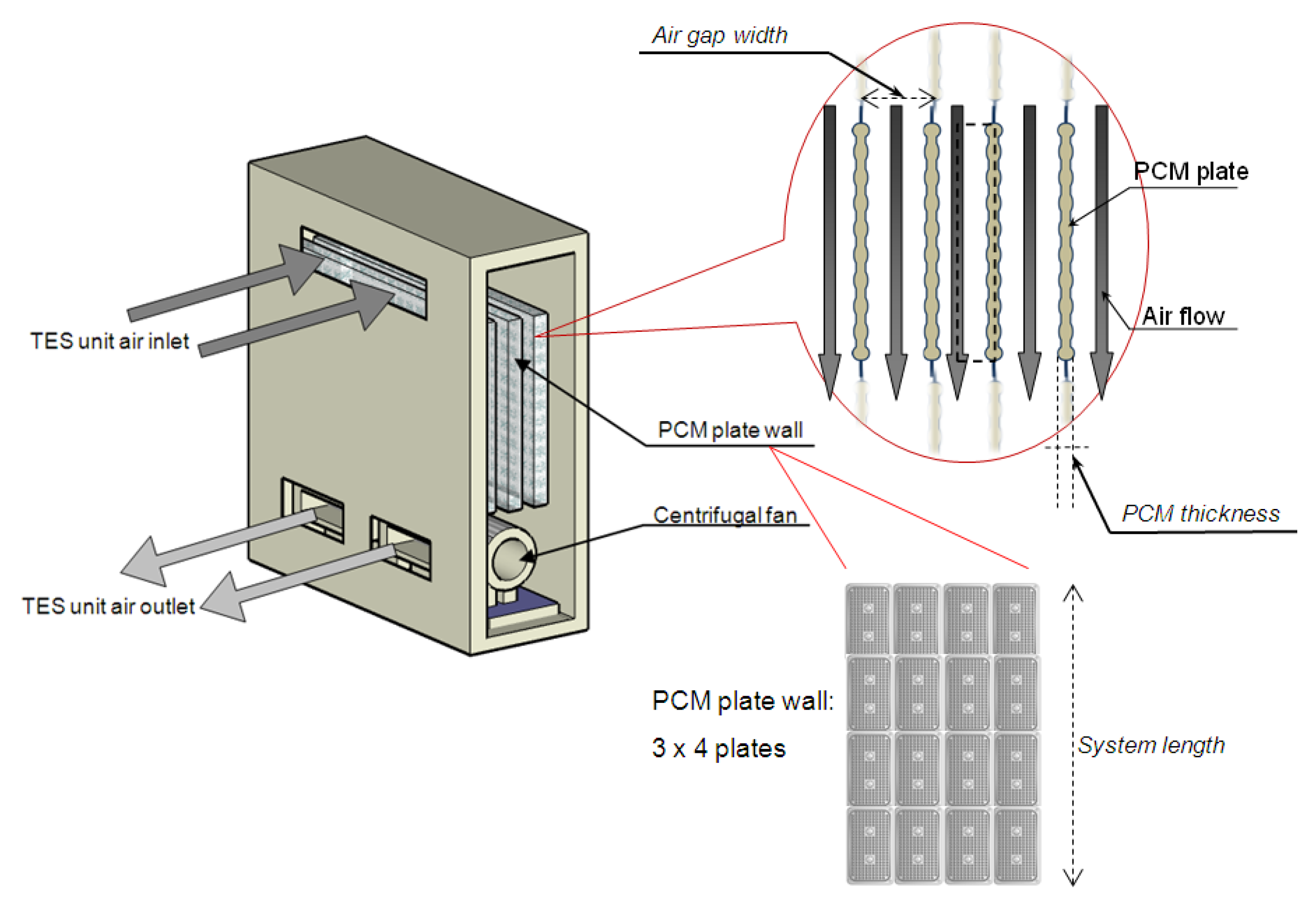
  • Number of plate walls is set at 18 (the same number as in the experimental prototype).
  • The only PCM considered was the commercial one used in the experimental prototype: RT27 (Rubitherm [29]).
  • Finishing of the simulated plates is the same as the plates in the prototype (round bulges).
  • Heat generation of the fan is considered constant and equal to 300 W.
It should be remarked that there is a dependent variable, the TES unit width (w), which is determined by the relation described in Equation (8):
  w = M P C M ρ P C M · 1 L s i s t · N · e p l a t e
Any action taken will affect not only the thermal behavior of the unit but also other important aspects, such as the initial investment, operating cost, electrical consumption, pressure drop, noise, weight, and floor space. In particular, we will focus on the following three responses:
  • Air maximum temperature, Tmax.
  • Pressure drop (necessary to determine which fan to use, electrical consumption, and noise), Δp.
  • PCM melting degree for design conditions, ° Melt.
Furthermore, given their interest, the following additional two calculations will be made:
  • Width of the TES unit (along with the length and depth allowing the floor space and the volume occupied by the unit to be calculated).
  • Maximum heat transfer rate supplied by the TES unit,   Q ˙ m a x .
The ambient temperature curve used in the numerical simulations corresponds to the data recorded by the solar cooling installation at the University of Zaragoza (Spain) on a hot day in July. Table 2 lists the selected factors and their domains expressed as minimum and maximum values.
  • The amount of PCM has to be theoretically sufficient for the stored energy to cover the needs of the average heat rate (13 kW);
  • Demand: 13 kW during eight hours 374,400 kJ;
  • Mass of RT27 required to cover the demand: hsl = 179 kJ/kg (which corresponds to the PCM latent heat in the thermal window of 20 to 32 °C) 2092 kg.
Table 2. Selected factors and their domain.
FactorsDomain
Level (−)Level (+)
PCM mass (kg)10003000
Length of the plate system (m)15
Thickness of the PCM plate (mm)515
Thickness of air duct gap (mm)555
Considering 2000 kg of PCM as a central value, the PCM mass factor will range between a lower level of 1000 kg and a higher level of 3000 kg. If the system is efficient, reducing the amount of PCM will be of interest (lower investment cost). Otherwise, it may be necessary to add more PCM to meet the requirements of temperature reduction (since we are not considering the modification of the PCM thermo-physical properties).
  • The length of the plate system is one of the two dimensions that will determine the unit’s floor space. Depending on the location of the unit (on the roof or inside ducts), this value will depend on the available space. In this case, for the factor length, we have selected a lower level of 1 m and a higher level of 5 m (that allows the placement on the roof with sufficient room).
  • The plate thickness is set at a lower level of 5 mm and a higher level of 15 mm. This value of maximum thickness should always obey the relation L/e > 10 in order to assume one-dimensional conduction (in this specific case 1000/15 = 66.6 >> 10).
  • The air gap has a lower level of 5 mm and a higher level of 55 mm. The idea behind this is to leave ample room to find a trade-off between compactness on the one hand and a small pressure drop on the other.
Once the factors have been determined, the design of experiments is set out using a central composite response surface of four factors. This has been achieved by using the statistical analysis software package Minitab 15 [30] that enables the simulations plan to be obtained. This plan comprises a structured and easily understandable list of simulations (instead of experiments) to be performed. Generally, this kind of list immediately shows a series of designs that can be discarded directly due to their technical unfeasibility. In this case, some designs were rejected due to a high-pressure drop (more than 100 Pa) that would increase drastically the electrical consumption of the TES unit fan. Further information can be found in Dolado [26].

4. Results and Discussion

Although there are graphical tools available for results analysis which can also provide useful information for designers, such as the contour plot or the overlapped contour plot, this work is focused on multi-response optimization.

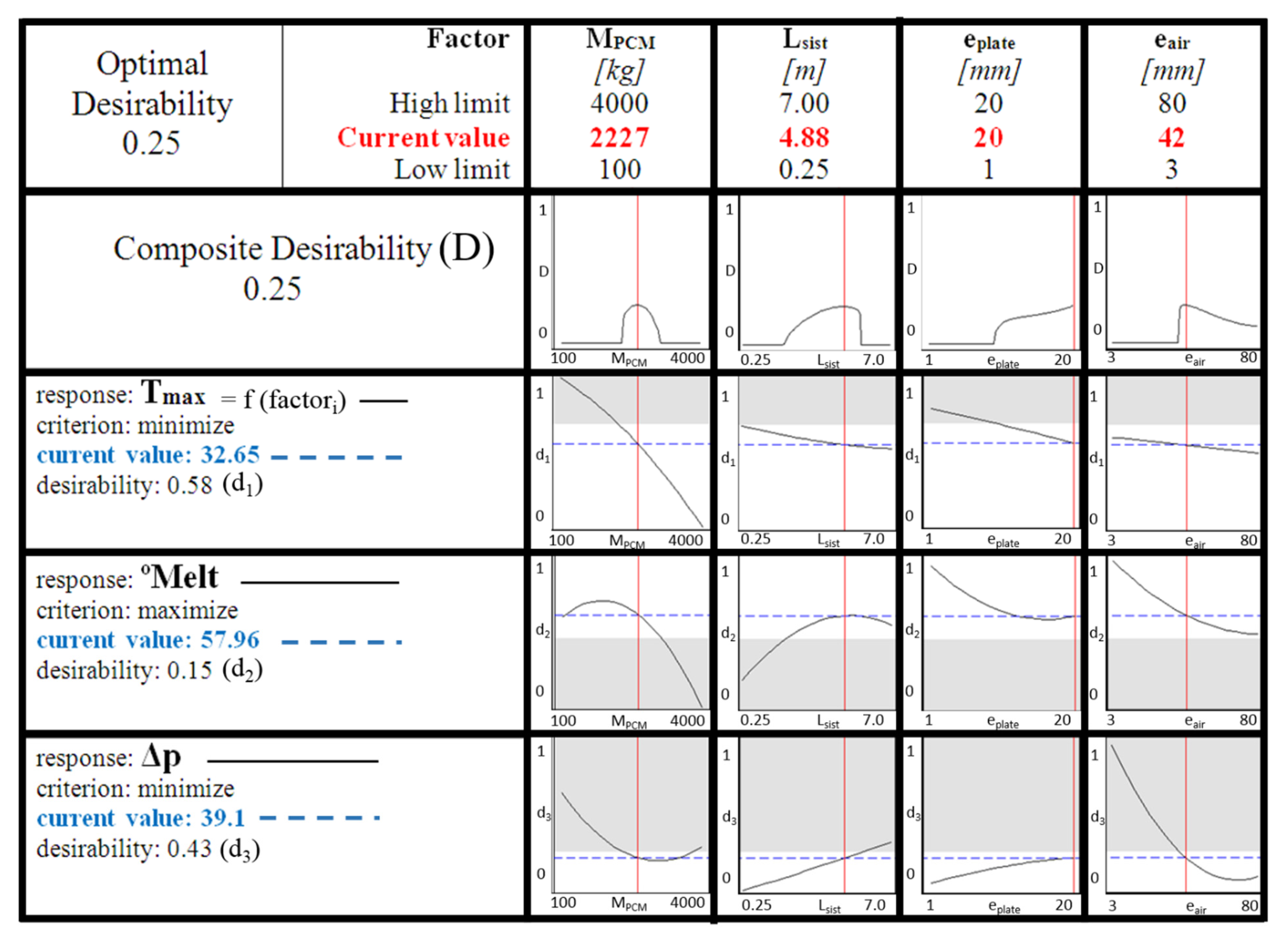
4.1. Response Optimization

This type of analysis is useful for identifying combinations of settings of input variables which together optimize a single response, or a response set. It is also useful for assessing the impact of multiple entries in the response. When the objective is to achieve several goals simultaneously or to meet certain requirements at the same time, using the response optimization methodology to find the combination of the input variable values allows optimal results to be achieved within the established acceptance range for each response.
The optimal response can be sought based on the criteria to be defined for each of the response variables: to minimize, to maximize, or to reach a target value. In this case study, the following three aspects have been established:
  • Minimizing the maximum temperature reached by the air (32 °C is the objective, the upper limit being 33.5 °C, which is 3 °C below the maximum outdoors temperature).
  • Maximizing the melting degree (i.e., efficiency) with the objective of minimizing the amount of PCM, but accepting as a minimum an efficiency of 50%.
  • Minimizing the pressure drop reducing the electrical consumption, accepting values close to 25 Pa, but not beyond 50 Pa.
Table 3 shows the parameters used in the three responses selected for the solar cooling study case.
Table 3. Combination of parameters to create each desirability function of the study case.
ResponseGoalLowerTargetUpperWeightImportance
Tmax (°C)Maximum203233.515
°Melt (%)Maximum50100100110
Δp (Pa)Minimum1255011
First, for each response an individual desirability (d) is obtained using the goals and boundaries provided. As stated above, there are three goals to choose from:
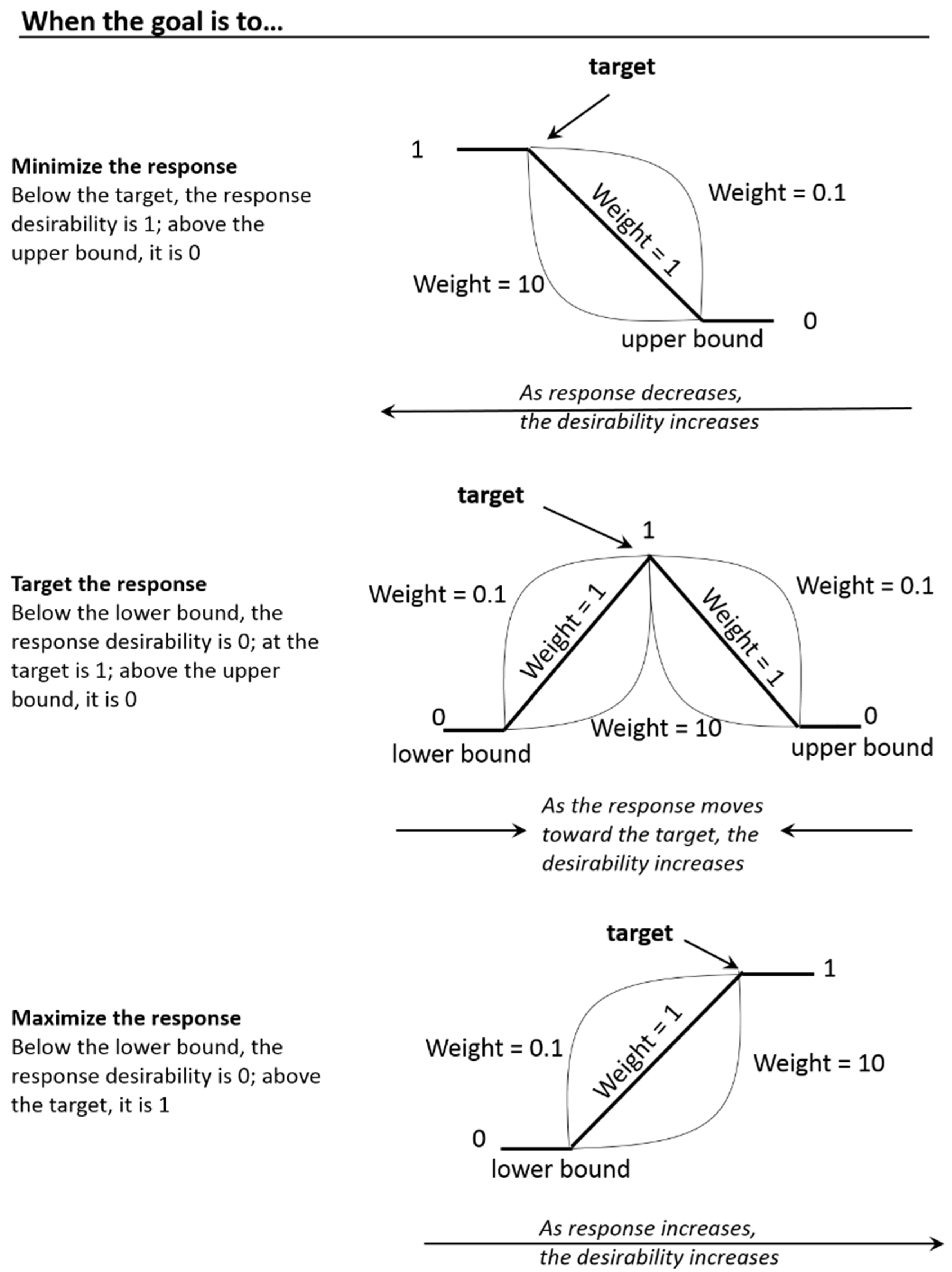
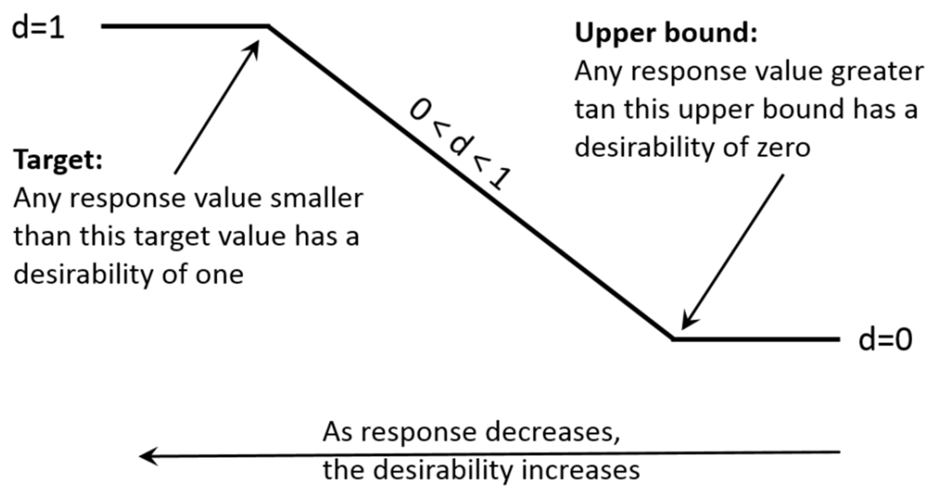
  • minimize the response,
  • target the response,
  • maximize the response.
For instance, suppose we have a response that we want to minimize. We need to determine a target value and an allowable maximum response value. The desirability for this response below the target value is one; above the maximum acceptable value, the desirability is zero. The closer the response is to the target, the closer the desirability is to one. Figure 3 shows the default desirability function (also called utility transfer function) used to determine the individual desirability (d) for a minimization goal:
Figure 3. Default desirability function for a minimization goal (adapted from [31]).
Resources 04 00796 g003
The shape of the desirability function between the upper bound and the target is determined by the choice of weight. Figure 3 shows a function with a weight of one.
After calculating the individual desirability for each response, they are combined to provide a measure of the composite, or overall, desirability of the multi-response system. This measure of composite desirability (D) is the weighted geometric mean of the individual desirabilities for the responses. The individual desirabilities are weighted according to the importance that we assign each response. The optimal solution (optimal operating conditions) can then be determined by maximizing the composite desirability.
Finally, to determine the numerical optimal solution, a reduced gradient algorithm with multiple starting points that maximizes the composite desirability is employed (optimal input variable settings). In order to calculate the numerical optimal solution, specification of a target and lower and/or upper bounds for each response is needed. The boundaries required depend on the goal (minimize, target, or maximize). In the approach to optimization, each of the response values are transformed using a specific desirability function. The weight determines how the desirability is distributed on the interval between the lower (or upper) bound and the target. It determines the shape of the desirability function that is used to translate the response scale to the zero-to-one desirability scale to determine the individual desirability of a response. A weight of one can be considered as a neutral setting. Increasing the weight requires the response to move closer to the target to achieve a specified desirability. Decreasing the weight has the opposite effect. The weight selection (from 0.1 to 10) emphasizes or de-emphasizes the target. A weight:
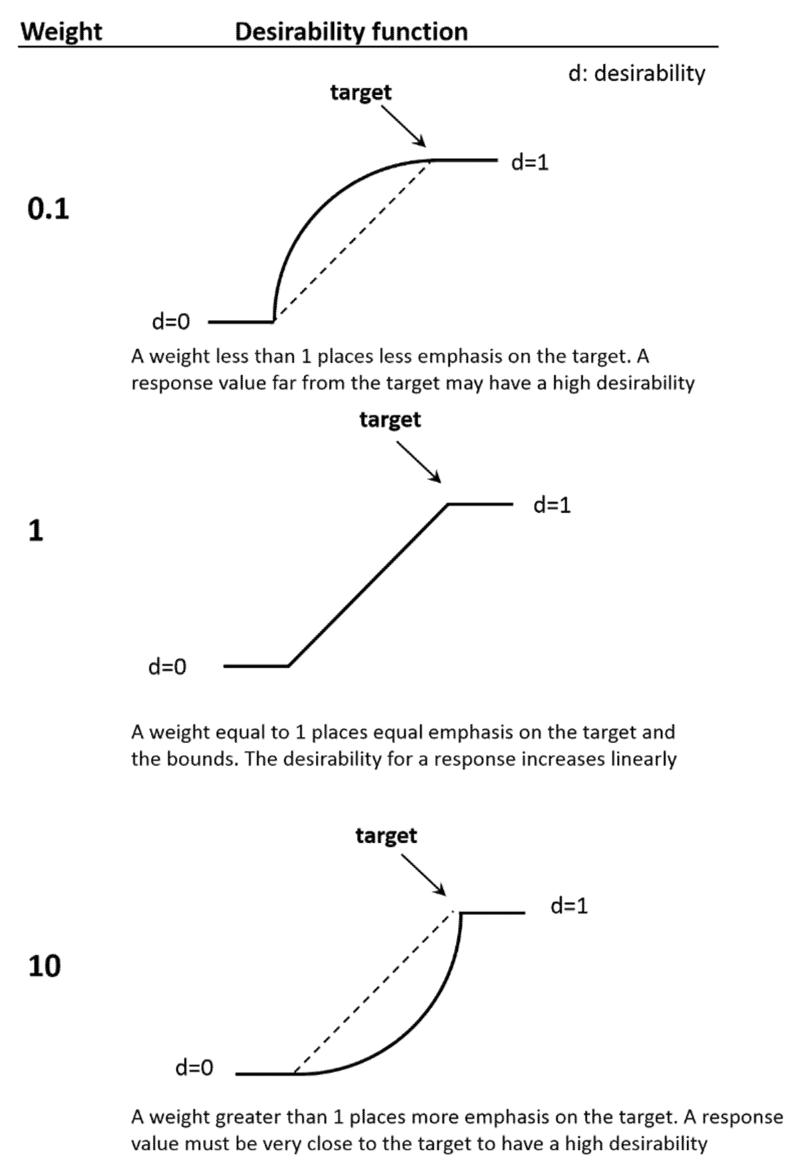
  • less than 1 (minimum is 0.1) places less emphasis on the target,
  • equal to 1 places equal importance on the target and the bounds,
  • greater than 1 (maximum is 10) places more emphasis on the target.
For instance, Figure 4 shows how the shape of the desirability function changes depending on the weight when the goal is to maximize the response.
Figure 4. Shape of the desirability function changes depending on the weight (adapted from [31]).
Resources 04 00796 g004
Figure 5 summarizes the desirability functions depending on the goal and the weight.
In the optimization of the present case study, assigning a value to the importance is based on the following criteria: we put the emphasis on having a unit as efficient as possible (10), which also ensures a significant reduction in the peak temperature (5), and preferably involving a pressure drop that is not too high (1).
Figure 5. Summary of desirability functions shapes (adapted from [31]).
Resources 04 00796 g005
After calculating the individual desirability of every single response and once these are weighted according to the importance attached to them, the values are combined to determine the composite desirability of the multi-response system. The Minitab Response Optimizer tool [30] is used to show how different experimental settings affect the predicted responses for the response surface design. Minitab calculates an optimal solution and draws the optimization plot. The optimal solution serves as the starting point for the plot (the settings can be modified interactively to see how different settings affect responses). The optimization plot (Figure 6) is very useful in terms of design, as it allows adjusting the values of the input variables and simultaneously seeing the effects of these changes in the responses, without running more simulations. The optimization plot reported shows the effect of each factor (columns) in the responses as well as in the composite desirability (rows). In each sub-plot, the vertical red lines represent the current value (which initially corresponds to the optimum one). The numbers in bold red at the top of the columns represent the current values of the factors (in the figure, these correspond to the optimal values). The horizontal blue lines and the blue numbers represent the responses for the selected levels of the factors. The grey area of each sub-plot indicates that the composite desirability is zero for the factor values within the corresponding range. The value of the composite desirability varies between zero and one (the unity represents the ideal case and the zero indicates that one or more responses are outside the acceptable limits).
Figure 6. Optimization results.
Resources 04 00796 g006
What is interesting about the optimized results is the value of the composite desirability as well as its trend according to each of the factors considered. The value obtained for the composite desirability is 0.25. This fact (far from unity) indicates that the values determined by the optimization are far from fulfilling the demanding requirements of the response variables. Furthermore, observing the single values, the efficiency is the response less satisfied (d = 0.15). In order to enhance the performance, other design factors (such as the surface rugosity (i.e., finishing), the number of plate-walls, or even the airflow) could be included in a further analysis. For the sake of simplicity and clarity, they are not reported here. Looking at the different trends of each sub-plot in Figure 6, it can be seen that there is always a trade-off between the three responses due to the effect of each factor. As an example, as the length of the system increases, the temperature reached by the air will be lower (advantage) but the pressure drop will increase (drawback); in the meantime, the melting degree will find a maximum within the length domain.

4.2. Suggested TES Unit

Once the optimal values are obtained, the theoretical model is run again to test the results and to acquire the heat rate curve. The values to be considered will not be the optimal ones, but realistic values close to them. These values have to be easier to handle, under the criteria of the manufacturing process, installation, handling, own experience, etc. The suggested TES unit works at 5500 m3/h, with 2200 kg of RT27 arranged in plates of 20 mm thickness and air channels of 40 mm. The plate system length is 4.9 m.
The main results obtained with the theoretical model running this unit are shown in Table 4. With this arrangement, a maximum heat transfer rate of 10.2 kW is achieved, and a pressure drop of 63 Pa. The unit's floor space is about 7.75 m2 and its volume is 8.4 m3. The results obtained from the simulation fit quite well with those predicted by the optimization in terms of Tmax, although they are somewhat better for the efficiency and show higher values for the pressure drop. However, it is also shown that the simulation follows the trends predicted by the optimization as, in the simulation, a smaller amount of PCM (increased efficiency) and a narrower air gap (increased Δp) have been considered compared to the optimal values.
Table 4. Simulation results obtained running the model with the suggested values.
MPCM (kg)Lsist (m)eplate (mm)eair (mm) Q ˙ m a x (W)Tmax (°C)vair (m/s)w (m)°Melt. (%)Δp (Pa)
22004.920401025732.91.431.4866.0763

4.3. Dimensional Analysis and Similarity

To check the degree of similarity between the experimental equipment and the different cases studied in the numerical simulations, the following dimensionless groups that characterize the process were calculated (Re, NTU, Bi, λeff/λ ratio). The range of experimental validity is shown in Table 1. Figure 7 shows the results of the calculation of every parameter for each simulation. In these plots, what is reported is whether or not each of the units simulated according to the DOE plan (diamonds) matches the validity range (grey zone), and in particular if the suggested design (circle) does so.
The response surface analysis of four factors and three main responses requires 31 experiments (i.e., simulation cases). The differences of each simulation case are shown in Table 5 and are devoted to the different values of the four factors considered in the study (PCM mass, system length, thickness of the PCM plate and air gap between PCM plates).
The analysis of these results reflects that natural convection within the PCM is going to play an important role in the suggested unit. This is because the λeff/λ ratio obtained is high, mainly due to the thickness of the selected PCM (20 mm). Re is also outside the experimental validity range. As the airflow is set, reconciling the application requirements with the adjustment of the Re to the experimental validity range is only achievable through the hydraulic diameter. Since the theoretical model itself takes into account both the effective thermal conductivity as well as the different flow regime, it seems reasonable to extrapolate by means of the simulations outside the experimental validity range. However, to be fully rigorous, the suggested unit proposed here would require additional experimentation for empirical validation, although the Bi and the NTU are within the experimental validity range. Therefore, it is concluded that the analysis performed for this solar cooling application is useful for a pre-design stage and, once validated with additional experimentation, would also be valid in a design stage.
Table 5. Simulation plan and corresponding responses for each of the 31 cases.
#Simulation planResponses
MPCM (kg)Lsist (m)eplate (mm)eaire (mm) Q ˙ m a x (W)Tmax (°C)vair (m/s)Width (m)°Melt (%)Δp (Pa)
11000155822736.21.3312.7774.09117
2300015515,50034.50.4438.3165.3456
3100055511,93536.36.652.55100170
4300055515,50134.52.227.6665.34150
5100051555738536.33.994.2671.75120
630005155512,67331.81.3312.7751.83115
710031030762136.319.940.8573.02250
840003103016,08532.36.652.5567.65180
920000.251030391234.20.1212.7747.0025
10200071030931031.20.0438.3138.6325
1120003130754336.20.602.5572.9127
12200032030933431.10.207.6638.7226
1320003103428434.20.364.2650.2925
14200031080483033.50.1212.7720.1325
15200031030484434.21.810.8555.9953
1620003103011,54331.20.602.5547.2027
17200031030107736.313.290.2161.59185
1820003103010,60830.40.338.5233.1627
19200031030640032.70.0651.0839.2430
2020003103012,22235.41.551.8270.6976
2120003103013,96735.10.0742.5787.9931
22100051555955333.11.332.1356.5437
2330005155514,79135.56.654.2690.19230
2410031030786532.30.254.2647.4925
2540003103010,59234.20.664.2662.6128
2620000.25103010,59234.20.664.2662.6128
2720007103010,59234.20.664.2662.6128
282000313010,59234.20.664.2662.6128
2920003203010,59234.20.664.2662.6128
302000310310,59234.20.664.2662.6128
3120003108010,59234.20.664.2662.6128
Figure 7. Re numbers (a); Bi numbers (b); NTU numbers (c); and λeff/λ ratio (d) for each simulation and experimental validity.
Resources 04 00796 g007

4.4. Evaluation of the System Performance During the Operation Period (Cooling)

The performance of the system has been evaluated during its operation after the incorporation of the TES unit. The hourly temperature data for Zaragoza, Spain (obtained from the TRNSYS 16 database [32]) have been considered as input values to the theoretical model. The analysis was performed for the four months in which the facility is operational (June–September). To accelerate the simulations a step function for the inlet air temperature has been used, with 1 min time steps. The average COP obtained for this configuration is 0.583 (the COP corresponds to the fitting reported by Monne et al. [28] as a function of inlet ambient temperature). Therefore, compared to the 0.51 measured [33], the incorporation of the TES unit would improve the average COP value by around 14%. Table 6 summarizes the overall results of the simulations. It reflects the significant reduction in the number of hours that the condensing unit of the absorption system is running with inlet air temperatures above 27 °C when the TES unit is incorporated in the system.
Table 6. Global results summary with and without the suggested TES unit.
System setupAverage COPHours working with T > 27 °C
without TES0.51456
with TES0.583399.3

4.5. Initial Investment Evaluation

A simple estimation of the investment cost has been done regarding the TES unit. Various points have been considered. If the TES unit can operate with the same fan as used by the condensing unit, the fan cost can be ignored. Another aspect to take into account is that the production scale is crucial in determining the costs of ordering material. If production is at an industrial level, this will lower the costs. Rubitherm, the manufacturer of the PCM plates [29], has confirmed reductions in the price of the macroencapsulated PCM for orders over 30,000 units (about 18,300 kg of RT27), negotiable between 8 and 18 €/kg. The price of this item will also be influenced by the encapsulation, the conformation material, itself, as well as the geometry and the manufacturing process. The casing of the TES unit is built on a folded and bolted steel plate. Taking into account all the material and labor costs, the cost of each casing depends on the final dimensions. An indicative order of magnitude depending on the volume occupied by the PCM in the TES unit is shown in Table 7. The criterion for selecting the fan was minimizing the consumption. The software Proselecta and Ventil developed by Nicotra-Gebhardt [34] has been used to select the fan, to set the airflow and to set the pressure drop. The fan with the lowest electrical consumption was chosen. In this case, as the air flows between plates with a narrow gap, centrifugal fans should be selected because the pressure drop can be significant. Table 8 shows the costs of these fans.
Table 7. Order of magnitude of the TES unit casing cost as a function of the PCM volume inside the unit.
Volume (m3)Cost (€)
0.5174
1.3376
2.0658
Table 8. Order of magnitude of centrifugal fan cost as a function of airflow.
Flow (m3/h)TypeConsumption (W)Cost (€)
2000RER10 11-315290547
5000RER10 11-384450591
8000RER10 11-577720837
The total investment cost of a TES unit with 2200 kg of RT27 (Rubitherm CSM (Compact Storage Module) format plates at the current minimum order price) and 5500 m3/h is estimated at 47,460 €. This value is highly restrictive so that in these conditions it will not be economically feasible. To make the TES unit competitive against conventional equipment in terms of initial investment, the price of the macroencapsulated PCM would have to be reduced down to about 5 €/kg. This can be deduced from Equation (9) that shows the linear relation between the unit initial investment costs (y) depending on the price of the macroencapsulated PCM in aluminum plate (x). Only a reduction in the price of the macroencapsulated PCM to the lowest values (5 €/kgPCMencapsulated) would establish a scenario in which the investment cost of the TES unit would be economically competitive compared to conventional cooling equipment.
y [ k ] = 1.82 x [ / k g ] + 5.91
Currently the price of bulk RT paraffins is between 3.80 and 5.00 €/kg; that means a Rubitherm CSM cost of 13 €/plate (at low scale production). The plate contains about 610 g of RT27, which implies a PCM cost between 2.32 and 3.05 €/plate. Therefore, the PCM is between 18 and 23% of the total cost of the plate. Thus, it seems advisable to focus not only on the reduction of the PCM price itself but also on the encapsulation material, as well as the encapsulation manufacturing process.
Alternatively, to achieve financial feasibility other factors can be included in the analysis (another PCM with better properties, modifying the PCM thermo-physical properties, etc.) that can improve the performance of the TES unit. However, none of these would result in the 2/3 PCM reduction required to make it viable. Furthermore, an empirical validation would be required with such modifications. The search for so-called low cost PCM and achieving cost effectiveness by improving PCM thermo-physical properties remain areas for future research.

5. Conclusions

Once an empirically-validated numerical model is obtained, the methodology proposed in this paper can be used in the design stage of a TES unit which is to be incorporated in a specific application. The methodology is useful for the following:
  • Reducing the number of simulation runs and the time invested. In the case study described in this paper, each numerical simulation corresponds to one single cycle at most (with a duration of two to six minutes per run on an average desktop computer), and only the behavior of the TES unit is simulated. Simulations of buildings are usually for one-year periods and include a complete system: an annual simulation with a simple system, a building and incorporating the TES unit can last 12 h with the numerical model.
  • Provided you have a PCM-TES numerical model empirically validated, the methodology can:
    -
    Adapt the design of the TES unit depending on the final requirements (responses) and in accordance to a series of variables or parameters (factors) influencing the system.
    -
    Find optimal points of operation based on multi-response functions criteria. These functions can be shape-defined by the designer depending on their goal (maximization of the function, minimization, or target objective), their weight, and their importance. This is done through desirability functions. In the approach to optimization, each of the response values are transformed using a specific desirability function. The weight determines how the desirability is distributed on the interval between the lower (or upper) bound and the target. It determines the shape of the desirability function that is used to translate the response scale to the zero-to-one desirability scale to determine the individual desirability of a response. In addition, the individual desirabilities are weighted according to the importance that we assign each response.
    -
    A key feature is that without having to run more numerical simulations, a designer can identify the factor settings that enable any other requirements to be fulfilled.
The DOE methodology has been applied to numerical simulations in a case study of solar cooling equipment, resulting in a theoretical improvement over the original design. An improvement in the COP of 14% has been obtained compared to the same system without a TES unit.
In order for these systems to be economically viable, a significant reduction in the price of the macroencapsulated PCM is necessary, mainly in terms of the encapsulation process rather than the cost of the PCM itself. Currently, an RT27 plate macroencapsulated by Rubitherm (as CSM panels) has a price of 13 € which makes the initial investment in this TES units highly restrictive in financial terms. A price reduction from the current 21.3 €/kg for macroencapsulated PCM (the price at small scale production) down to at least 5 €/kg would be required for the initial investment to be competitive, which is relatively close to the 8€/kg achievable nowadays by the manufacturer, depending on the production scale.
As the incorporation of the TES unit to support the solar cooling system has been considered, the possibility could also be examined of integrating a TES unit with a PCM phase changing at a lower temperature (about 10 °C) to act on the heating mode of a heat pump. In addition to an improvement in the COP, this would probably provide a reduction in the number of defrosting operations due to low temperatures. Other applications of interest could be free cooling or temperature maintenance in rooms.

Acknowledgments

The authors thank the Spanish Government for the partial funding of this work within the framework of research projects ENE2008-06687-C02-02, ENE2011-28269-C03-01 and ENE2014-57262-R. Special thanks are extended to Miguel Zamora, CIAT R&D Manager, for his collaboration. Recognition is also given to the fruitful collaboration within the joint Annex 29-Task 42 of the ECES/SHC Implementing Agreements of the IEA.

Author Contributions

This paper and the literature review it is partly based on the Ph. D. project of Pablo Dolado and further developed with the research group colleagues working on thermal energy storage: Javier Mazo, Ana Lazaro, Monica Delgado and Conchita Peñalosa. The advisory team is composed of Belen Zalba and Jose M. Marin.

Conflicts of Interest

The authors declare no conflict of interest.

Nomenclature, Acronyms and Definitions

A [m2]
area
cp [J/(kg·K)]
specific heat capacity at constant pressure
d
desirability parameter (ranges from 0 to 1)
Dh [m]
hydraulic diameter
eair [m]
thickness of the air gap between two PCM plates
eenc [m]
thickness of the plate encapsulation material
eplate [m]
thickness of the PCM plate
h [W/(m2·K)]
air convection coefficient
Lsist [m]
Length of the PCM system in the TES unit
m ˙ [kg/s]
mass flow
MPCM [kg]
PCM mass
N
number of PCM plate walls (inside the TES unit)
P [m]
wet perimeter
Q ˙ [W]
heat transfer rate
T [°C]
temperature
Tamb [°C]
outdoors air temperature
v [m/s]
velocity
V [m3]
volume
w [m]
width
°Melt
ratio of PCM melted, percentage
Δp [Pa]
pressure difference
λ [W/(m·K)]
thermal conductivity
λeff [W/(m·K)]
effective thermal conductivity
ρ [kg/m3]
density
µ [Pa·s]
dynamic viscosity
Bi = h·e/λenc
Biot number
C a i r = ρ a i r · V ˙ 2 · N · c p a i r
heat capacity [J/(s·K)]
Re, = ρ·v·Dh
Reynolds number
NTU = (h·Δx·w)/Cair
number of transfer units
COP
Coefficient of Performance
CSM
Compact Storage Module
DOE
Design of Experiments
PCM
Phase Change Material
TES
Thermal Energy Storage

References

  1. Pérez Vergara, I.G.; Díaz Batista, J.A.; Díaz Mijares, E. Experimentos de simulación utilizando superficies de respuesta para su optimización (Simulation experiments using response surfaces for optimization). Cent. Azúcar 2001, 2, 68–74. [Google Scholar]
  2. Del Coz Díaz, J.J.; García Nieto, P.J.; Lozano Martínez-Luengas, A.; Suárez Sierra, J.L. A study of the collapse of a WWII communications antenna using numerical simulations based on design of experiments by FEM. Eng. Struct. 2010, 32, 1792–1800. [Google Scholar]
  3. Gunasegaram, D.R.; Farnsworth, D.J.; Nguyen, T.T. Identification of critical factors affecting shrinkage porosity in permanent mold casting using numerical simulations based on design of experiments. J. Mater. Process. Technol. 2009, 209, 1209–1219. [Google Scholar]
  4. Antony, J. Training for design of experiments using a catapult. Qual. Reliab. Eng. Inter. 2002, 18, 29–35. [Google Scholar] [CrossRef] [Green Version]
  5. Dolado, P.; Lázaro, A.; Marín, J.M.; Zalba, B. Characterization of melting and solidification in a real scale PCM-air heat exchanger: Numerical model and experimental validation. Energy Convers. Manag. 2011, 52, 1890–1907. [Google Scholar] [CrossRef]
  6. Doehlert, D.H. Uniform shell designs. J. R. Stat. Soc. Ser. C 1970, 19, 231–239. [Google Scholar] [CrossRef]
  7. Myers, R.H.; Montgomery, D.C. Response Surface Methodology: Process and Product Optimization Using Designed Experiments; Wiley: New York, NY, USA, 1995. [Google Scholar]
  8. Beyer, H.; Sendhoff, B. Robust optimization—A comprehensive survey. Comput. Methods Appl. Mech. Eng. 2007, 196, 3190–3218. [Google Scholar] [CrossRef]
  9. Dellino, G.; Kleijnen, J.P.C.; Meloni, C. Robust optimization in simulation: Taguchi and response surface methodology. Inter. J. Prod. Econ. 2010, 125, 52–59. [Google Scholar] [CrossRef] [Green Version]
  10. Dessouky, Y.M.; Bayer, A. A simulation and design of experiments modeling approach to minimize building maintenance costs. Comput. Ind. Eng. 2002, 43, 423–436. [Google Scholar] [CrossRef]
  11. Ramakrishnan, S.; Tsai, P.F.; Srihari, K.; Foltz, C. Using Design of Experiments and Simulation Modeling to Study the Facility Layout for a Server Assembly Process. In Proceedings of the 17th Annual Industrial Engineering Research Conference, Vancouver, B.C., Canada, 17–21 May 2008; pp. 601–606.
  12. Zalba, B. Thermal Energy Storage with Phase Change: Experimental Procedure. Ph.D. Thesis, University of Zaragoza, Zaragoza, Spain, 10 April 2002. [Google Scholar]
  13. Zalba, B.; Sánchez Valverde, B.; Marín, J.M. An experimental study of thermal energy storage with phase change materials by design of experiments. J. Appl. Stat. 2005, 32, 321–332. [Google Scholar]
  14. Gunasegaram, D.R.; Smith, B.J. MAGMASOFT helps assure quality in a progressive Australian iron foundry. In Proceedings of the 32nd National Convention of the Australian Foundry Institute, Fremantle, Australia, 20–23 October 2001; pp. 99–104.
  15. Calise, F.; Palombo, A.; Vanoli, L. Maximization of primary energy savings of solar heating and cooling systems by transient simulations and computer design of experiments. Appl. Energy 2010, 87, 524–540. [Google Scholar]
  16. Gupta, A.; Ding, Y.; Xu, L.; Reinikainen, T. Optimal parameter selection for electronic packaging using sequential computer simulations. J. Manuf. Sci. Eng. 2006, 128, 705–715. [Google Scholar] [CrossRef]
  17. Whitt, W. Analysis for the Design of Simulation Experiments; Columbia University: New York, NY, USA, 2005. [Google Scholar]
  18. Salazar, J.C.; Baena Zapata, A. Analysis and design of experiments applied to simulation studies. Dyna Bilbao 2009, 76, 249–257. [Google Scholar]
  19. Vanderplaats, G.N. Numerical Optimization Techniques for Engineering Design: With Applications; McGraw-Hill: New York, NY, USA, 1984. [Google Scholar]
  20. Jaluria, Y. Design and Optimization of Thermal Systems, 2nd ed.; CRC Press: Boca Raton, FL, USA, 2008. [Google Scholar]
  21. Nocedal, J.; Wright, S.J. Numerical Optimization, 2nd ed.; Springer Science: New York, NY, USA, 2006. [Google Scholar]
  22. Dolado, P.; Lázaro, A.; Marín, J.M.; Zalba, B. Characterization of melting and solidification in a real-scale PCM-air heat exchanger: Experimental results and empirical model. Renew. Energy 2011, 36, 2906–2917. [Google Scholar] [CrossRef]
  23. Lázaro, A.; Dolado, P.; Marín, J.M.; Zalba, B. PCM-air heat exchangers for free-cooling applications in buildings: Experimental results of two real-scale prototypes. Energy Convers. Manag. 2009, 50, 439–443. [Google Scholar] [CrossRef]
  24. Lázaro, A.; Dolado, P.; Marín, J.M.; Zalba, B. PCM-air heat exchangers for free-cooling applications in buildings: Empirical model and application to design. Energy Convers. Manag. 2009, 50, 444–449. [Google Scholar] [CrossRef]
  25. Dolado, P.; Mazo, J.; Lázaro, A.; Marín, J.M.; Zalba, B. Experimental validation of a theoretical model: Uncertainty propagation analysis to a PCM-air thermal energy storage unit. Energy Build. 2012, 45, 124–131. [Google Scholar] [CrossRef]
  26. Dolado, P. Thermal Energy Storage with Phase Change. Design and Modeling of Storage Equipment to Exchange Heat with Air. Ph. D. Thesis, University of Zaragoza, Zaragoza, Spain, 2011. [Google Scholar]
  27. Lebini, G. Solar cooling for small residential applications: Setup of “casetta di Cimiano” (laboratory) in Milan—The ISSA system. In Innovative solutions for building conditioning focus on solar cooling; Report of the ProEcoPolyNet Network project: Bergamo, Italy, 2008. [Google Scholar]
  28. Monne, C.; Alonso, S.; Palacin, F.; Guallar, J. Stationary analysis of a solar LiBr-H2O absorption refrigeration system. Inter. J. Refrig. 2011, 34, 518–526. [Google Scholar] [CrossRef]
  29. Rubitherm GmbH. Available online: http://www.rubitherm.com/ (accessed on 26 October 2015).
  30. Minitab. Downloads. Available online: http://www.minitab.com/en-us/downloads/ (accessed on 26 October 2015).
  31. Minitab User’s Guide 2: Data Analysis and Quality Tools, Release 13 for Windows; Minitab Inc.: State College, PA, USA, 2000.
  32. Trnsys. Available online: http://www.trnsys.com/ (accessed on 26 October 2015).
  33. Monne, C.; Alonso, S.; Palacin, F.; Serra, L. Monitoring and simulation of an existing solar powered absorption cooling system in Zaragoza (Spain). Appl. Therm. Eng. 2011, 31, 28–35. [Google Scholar] [CrossRef]
  34. Nicotra-Gebhardt. Pro-Selecta fan configurator. Available online: http://www.nicotra-gebhardt.com/en/infocenter/proselecta-ii.html (accessed on 26 October 2015).

