Article

Application of Machine Learning Algorithms to Predict Gas Sorption Capacity in Heterogeneous Porous Material

1
Computer Information Science Department, Universiti Teknologi PETRONAS, Seri Iskandar 32610, Perak, Malaysia
2
Department of Petroleum Geoscience, Faculty of Geoscience & Petroleum Engineering, Universiti Teknologi PETRONAS, Seri Iskandar 32610, Perak, Malaysia
3
Southeast Asia Clastic and Carbonate Research Laboratory, Department of Geoscience, Universiti Teknologi PETRONAS, Seri Iskandar 32610, Perak, Malaysia
4
Software Engineering Department, Mehran University of Engineering and Technology, Sindh, Jamshoro 76062, Pakistan
*
Author to whom correspondence should be addressed.
Resources 2025, 14(5), 80; https://doi.org/10.3390/resources14050080
Submission received: 24 April 2025 / Revised: 11 May 2025 / Accepted: 13 May 2025 / Published: 16 May 2025

Abstract

:
Shale gas is a clean and effective energy source that plays a big part in the transition from high-carbon to low-carbon energy, serving as a link for the growth of low-carbon energy in the future. Since shale rock is a heterogeneous porous material, the best production strategy is determined by a precise assessment of geological gas-in-place. Therefore, the economic and technical foresight of the production operations depends on the estimation of the adsorbed gas amount in shale resources. The isotherm curves of shale gas derived in this study were classified as type 1 isotherms, which indicates the presence of micropores in these samples. In this work, XGBoost (extreme gradient boosting) and ANN (artificial neural network) optimized with ABC (artificial bee colony) and PSO (particle swarm optimization) have been proposed to learn and then predict the methane sorption capacity (MSC) in shale based on total organic carbon (TOC), temperature, pressure, and moisture as input variables, with the gas adsorption amount of shale as the output. Statistical and graphical methods were used to compare the experimental results with the expected values. By comparison, the current work’s ANN-ABC and ANN-PSO models outperform all previous studies with higher R2 values (0.9913 and 0.9954) and lower RMSE scores (0.0457 and 0.0420), respectively, indicating improved predictive accuracy and generalization ability. The findings demonstrate that, in comparison to earlier models, the suggested models provide an exceptional prediction of the adsorbed gas amount in a heterogeneous porous medium. With additional data available, it may be easily updated for wider applications. Overall, this paper shows that machine learning can be used to forecast shale gas adsorption, and a well-trained model may be incorporated into a large numerical framework to optimize shale gas production curves.

1. Introduction

Shale gas, a methane-rich unconventional natural gas, significantly enhances global energy reserves [1,2]. In the U.S., the shale gas revolution, driven by long horizontal drilling and multistage hydraulic fracturing, has effectively addressed the energy gap [3]. Furthermore, shale gas reservoirs are regarded as green and eco-friendly resources that can increase energy efficiency [4,5]. Despite shale gas’s vast significance and its heterogeneity as a porous material, determining the amount of recoverable shale gas is fraught with uncertainty [6]. Assessing gas adsorption capacity is the initial step. In shale gas reservoirs, this capacity is a crucial factor that influences the assessment of gas-in-place (GIP) reserves and the production life of shale gas wells. Moreover, comprehensive information about gas adsorption, gas transport, and their interactions are required for shale gas production [7,8].
As of 2022, shale gas continues to play a significant role in the global energy mix. The U.S. Energy Information Administration [9] reports that shale gas accounts for approximately 78% of total U.S. dry natural gas production. Meanwhile, countries like China are investing heavily in shale development to meet their domestic energy demand and reduce dependency on coal [10]. Several countries, including Canada, China, the United Kingdom, India, Malaysia, and Spain, etc., continue to investigate the potential of shale gas due to its economic importance [11,12,13,14,15,16,17]. Nearly 80% of dry natural gas production in the U.S. in 2023 came from shale gas [18]. Recent studies have highlighted the critical role of shale gas in the global energy landscape. For example, Lin [19] highlights the significance of comprehending these mechanisms for effective resource extraction by discussing a variety of factors influencing gas adsorption behaviors in shale reservoirs. Hu [20] has created a dual-site Langmuir model to simulate high-pressure methane adsorption in shale, which sheds light on the thermodynamic parameters that are essential for simulating gas transport and storage in shale formations.
Natural gas is stored as dissolved and free gas, as well as adsorbed gas, in a shale gas reservoir [21,22]. Despite the increasing global trend toward shale gas, uncertainties exist about the estimation of recoverable gas and the estimate of adsorbed gas in the in situ state, which have an impact on well lifetime and GIP evaluation. [21,23]. Approximately 20–85% of the total shale GIP remains as adsorbed gas under reservoir conditions [24]; it highlights the significance of figuring out the adsorption capacity of natural gas. Porous material adsorption plays a pivotal role in shale gas reservoirs, significantly influencing both gas storage and recovery processes [25]. Recent studies have underscored the importance of adsorption in shale gas reservoirs [26]. In the context of reservoir modification, understanding the adsorption behavior is instrumental. Adsorption influences the effectiveness of techniques such as gas injection for enhanced recovery and CO2 sequestration [19].
Methane sorption capacity (MSC) tests on shale rocks have been conducted at various pressures and temperatures in order to develop a model for the accurate prediction of MSC in shale, which needs a range of experimental data. When creating a production plan, an accurate model can help determine the reservoir’s GIP [21,23].
Recently, ML (machine learning) approaches have been considered as tremendous alternatives for classical models when it comes to complex systems and heterogeneous porous material [27,28,29,30]. Several areas of petroleum engineering have also begun to use similar intelligent methods [31,32,33,34,35]. There are few studies employing black box ML models for the prediction of MSC. Meng [22] constructed several common ML models, which include RF (random forest), XGBoost (extreme gradient boosting), SVM (support vector machine), and ANN (artificial neural network). They utilized total organic carbon (TOC), temperature, moisture, and pressure as input variables, with excess adsorption amount of shale gas as the output. With a correlation coefficient (R2) of 0.9886 for the test subgroup, the results showed that the XGBoost model could outperform the others. In a further study, Syah [36] considered GWO-SVM (gray wolf optimizer support vector machine) to predict adsorbed gas. A data collection comprising pressure, temperature, humidity, and TOC was gathered from multiple sources for this purpose, and the GWO-SVM model was developed using it. According to the findings, this model’s R2 and Root Mean Squared Error are 0.982 and 0.08, respectively. Zhou [37] predicted MSC using the Gaussian Process Regression (GPR) model. Five common variables were taken into consideration: pressure, temperature, clay minerals, TOC, and moisture. A comparison was made between the GPR model’s performance and the widely used XGBoost model. It turned out that our GPR model had better accuracy for predicting MSC in shale, with an average relative error of less than 3%. Most recently, Chinamo [38] used PSO-SVR (particle swarm optimization–support vector regression), GWO-SVR, and SSA-SVR (sparrow search algorithm–support vector regression) models. The results showed that the PSO-SVR model is the most accurate in predicting MSC, with RMSE (Root Mean Squared Error) and R2 values of 0.09990 and 0.9605, respectively.
Even though shale gas adsorption predictions using ML techniques have shown comparatively good results, these techniques still require improvement. Therefore, to the best of our knowledge, this is the first time ANN and XGBoost, optimized with PSO and artificial bee colony (ABC), are developed for MSC prediction in heterogeneous porous materials, i.e., shale reservoirs. For this purpose, a dataset containing temperature, pressure, TOC, and moisture content has been collected from published sources, and the ANN and XGBoost, optimized with the PSO and ABC models, were created based on it. ANN-PSO, ANN-ABC, and XGBoost-ABC provided accurate predictions of MSC. Additionally, the findings confirm that, in comparison to earlier models, the suggested model provides an outstanding forecast of the amount of adsorbed gas. This study’s findings provide insight into the capabilities of ANN and XGBoost optimized with PSO and ABC modeling techniques, demonstrating that these models may be used to calculate MSC in shale gas formation with precise and user-friendly correlations. While previous studies have demonstrated the utility of models such as XGBoost and SVM in predicting methane adsorption in shale, these approaches often struggle with modeling highly nonlinear relationships inherent in heterogeneous porous media. Gradient boosting models rely heavily on feature engineering and decision tree structures, which may not capture complex hierarchical patterns effectively. In contrast, ANNs, particularly when optimized with swarm intelligence (SI) techniques like PSO and ABC, offer enhanced flexibility in learning nonlinear interactions. However, there is a lack of systematic comparative studies justifying the hybridization of ANN with SI for shale gas adsorption prediction. This study aimed to address that gap.

2. Methods

2.1. Aims and Workflow

The major purpose of the current research is to use two ML models, i.e., ANN and XGBoost algorithms, optimized by the PSO and ABC algorithms to be suitable in predicting MSC when exposed to heterogeneous porous material, i.e., shale rocks. Based on the available dataset from an open source [39,40], the input parameters are temperature, pressure, moisture content, gas adsorption of CH4, and TOC of shale, as shown in Figure 1. Since pressure is the most common measurement when all other parameters are maintained constant, this essentially provides a multicomponent adsorption isotherm that incorporates the influence of the other given factors and does not assume a specific relationship between sorption and pressure. The input data are normalized before being implemented in ANN-PSO, ANN-ABC, XGBoost-PSO, and XGBoost-ABC, and outputs are then realized and modified to adsorption capacity. The more details of the ML algorithm used in this study are explained in the following sections.

2.2. Machine Learning Base Models

In ML, the performance of models like XGBoost and ANN heavily depends on the optimal selection of hyperparameters. Metaheuristic optimization algorithms such as PSO and ABC are employed to fine-tune these hyperparameters, enhancing model accuracy and generalization. We have described the details of optimization steps in Section 3.2, while the general introductions of these algorithms are written as follows in Section 2.2.1, Section 2.2.2, Section 2.2.3 and 2.2.4. It is suggested that the cited articles be used to obtain the fundamental equations for these methods [41,42,43,44,45,46,47].

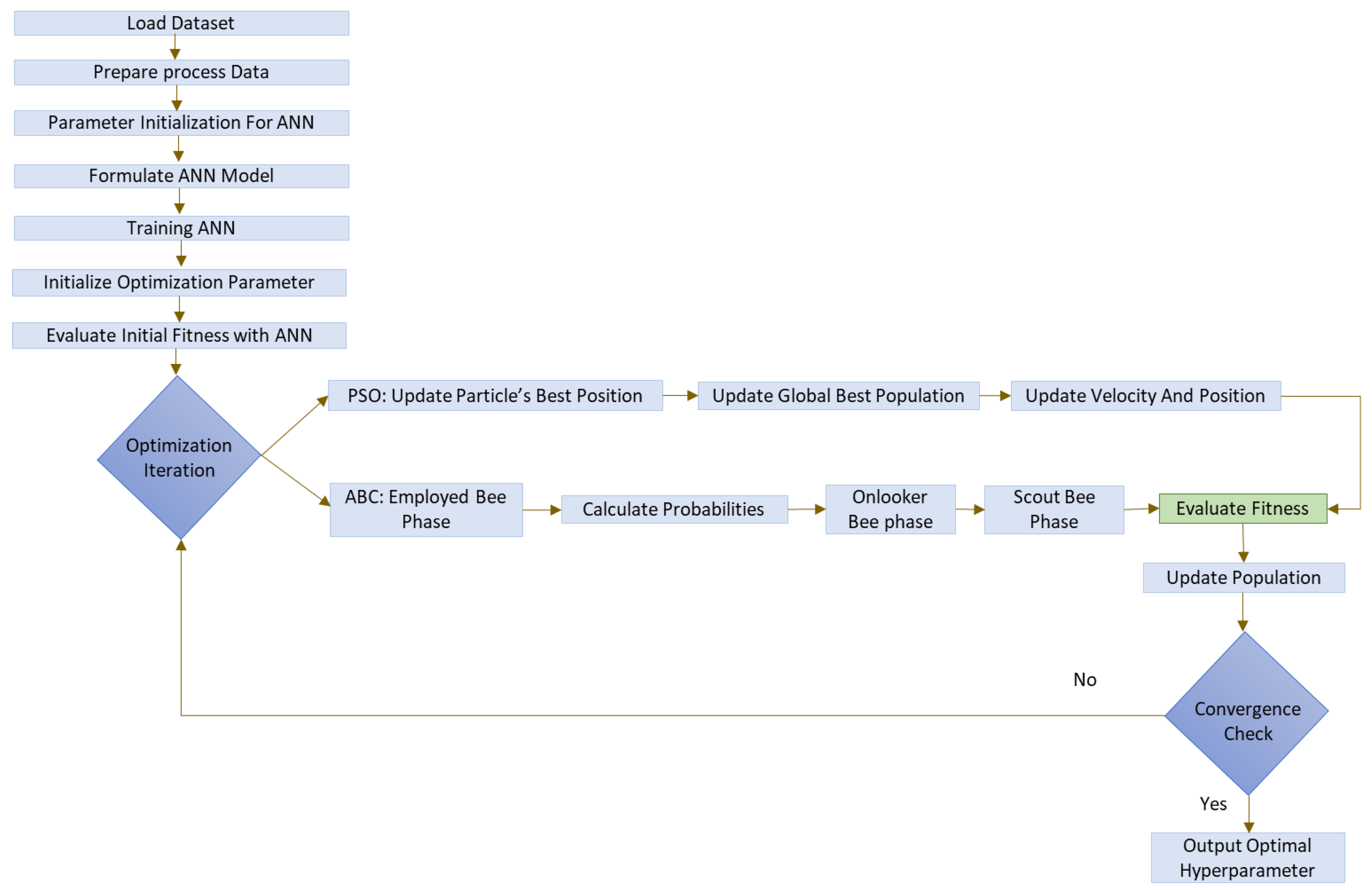
2.2.1. Artificial Neural Network (ANN)

Animal brain biological neural networks serve as the model for ANNs. It is an effective ML approach for issues involving both classification and regression. Deep neural networks have been used in a variety of domains, such as machine translation, autonomous driving, and speech recognition. One input layer, one or more hidden layers, and one output layer make up a standard ANN model [48]. Multiple nodes in each layer receive values from the predecessor nodes, use activation functions to compute, and then send the results to the successor nodes.

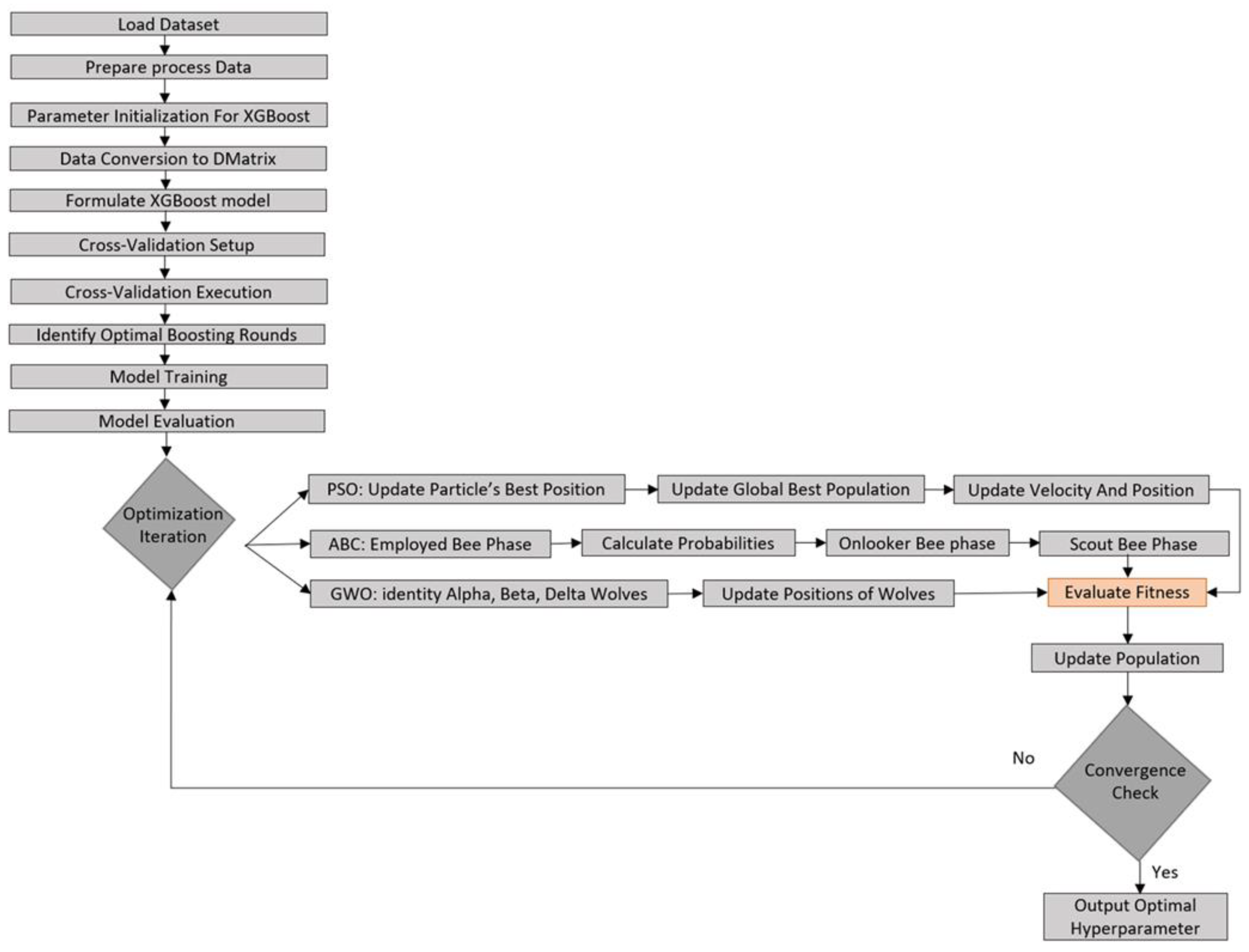
2.2.2. Extreme Gradient Boosting (XGBoost)

Data scientists frequently employ XGBoost, an open-source, scalable, end-to-end tree boosting system created by Chen and Guestrin, to obtain cutting-edge accuracy on a variety of classification and regression issues [42]. It has been demonstrated that XGBoost produces predictions more quickly and accurately than previous gradient boosting implementations. A method known as gradient boosting involves building new models that forecast the previous model’s residuals, which are then added together to determine the final choice. To reduce loss when adding new models, it employs a gradient descent approach.

2.2.3. Artificial Bee Colony (ABC) Optimization

ABC is a metaheuristic optimization method that draws inspiration from honeybee swarms’ intelligent foraging strategies. It was introduced by Karaboga [49,50]. ABC has become well known for its ease of use and efficiency in resolving a variety of optimization issues. Food sources and bee species are the two primary parts of ABC algorithms.

2.2.4. Particle Swarm Optimization (PSO)

The PSO algorithm is a stochastic, population-based algorithm that closely resembles evolutionary computation techniques like genetic algorithms based on animal social behaviors, such as flocking birds, schooling fish, and insects [51]. PSO finds the optimal solutions by updating generations after initiating a collection of random solutions known as particles. Similar to the “population” used in evolutionary systems like genetic algorithms, the accumulation of particles in PSO is referred to as the “swarm”. Particles in this approach follow the ideal particles as they fly through the problem space [52]. In other words, each particle in the swarm moves toward a new location in the D-dimensional search space based on the success of its topological neighbors. This makes the PSO an algorithm that uses a social psychology paradigm, where each particle interacts with its neighbors and the population as a whole [53].

2.3. Data Acquisition

The quality of the dataset that the model was trained on has a significant impact on the consistency and effectiveness of any suggested model. In this work, a large dataset of experimental measurements, including 352 measurements generated by Beaton et al. in 2008 and 2010, was used [39,40]. It should be noted that the dataset originates from Beaton, which focused on shale formations from a specific geographic region in Canada. As such, the model’s predictive scope may be geographically constrained. Figure 2 illustrates box plots for every parameter in the data databank to visualize the utilized data range and frequency. The box plot can provide useful statistical information about minimum, lower quartile (Q1), median (Q2), upper quartile (Q3), mean, minimum, and maximum values. Q1, marking the 25th percentile of the data, is the median of the lower half of the dataset, indicating that 25% of the data points are below this first quartile. Meanwhile, Q3, representing the 75th percentile of the data, is the median of the upper half of the dataset, signifying that 75% of the data points are below Q3 while 25% are above. The databank was randomly split into two subsets, the train and test subsets, with proportions of 80% and 20%, before moving on to the learning process. The model was trained using the training subset, and its ability to predict unseen data was assessed using the remaining data points.

3. Results and Discussion

3.1. Numerical Model for Shale Gas in Heterogeneous Porous Material

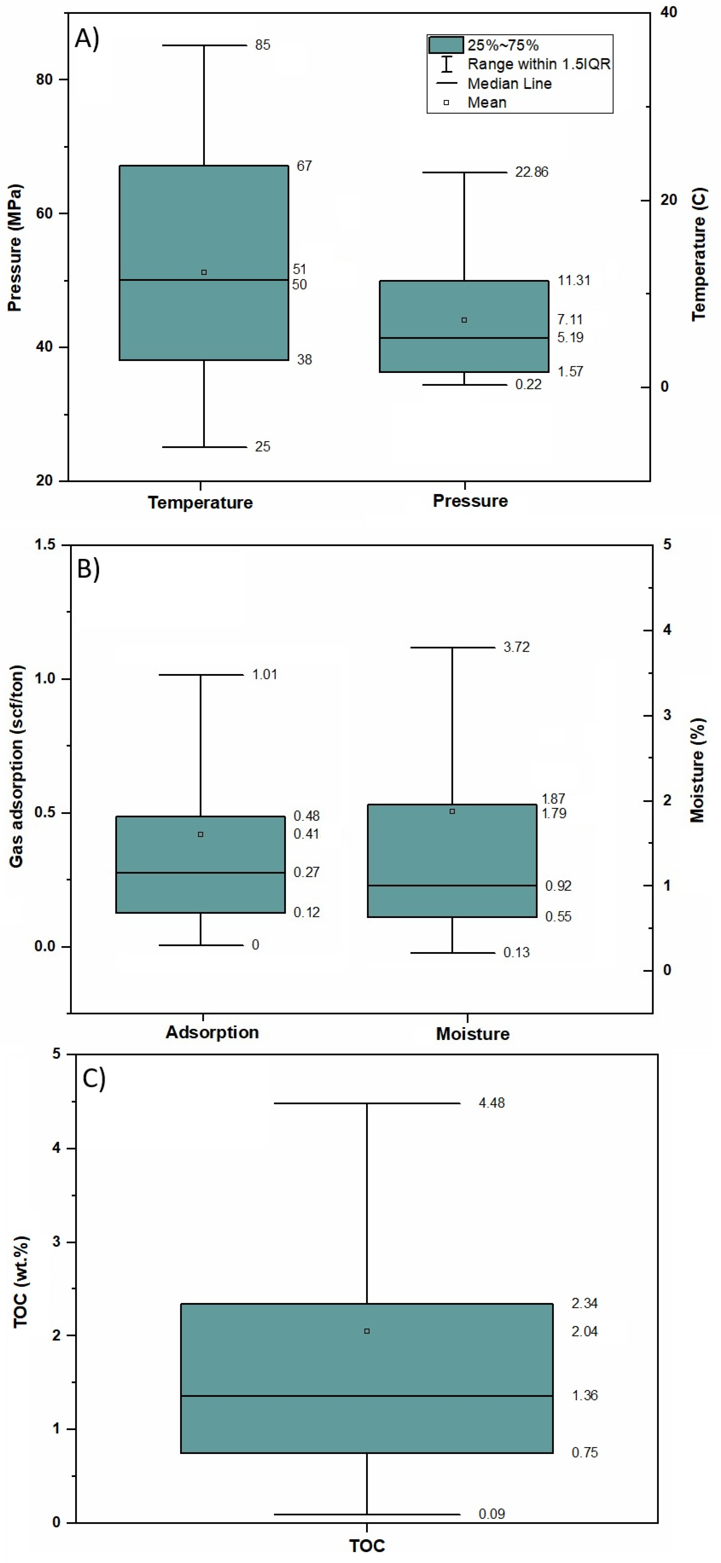
3.1.1. Input Variables and Output

Methane sorption in heterogeneous porous material, i.e., shale gas, is predominantly influenced by geochemical and thermodynamic conditions. TOC serves as a proxy for the adsorptive surface area, while temperature and pressure dictate gas behavior through adsorption isotherms. Moisture content affects sorption negatively by occupying adsorption sites. The output, MSC, quantifies the amount of methane adsorbed per unit mass of shale and is crucial for evaluating gas-in-place in shale reservoirs.
Input Features (X):
-
Total organic carbon (TOC, wt%).
-
Temperature (T, °C or K).
-
Pressure (P, MPa).
-
Moisture content (M, wt%).
-
Output (Y): Methane sorption capacity (MSC, mmol/g).

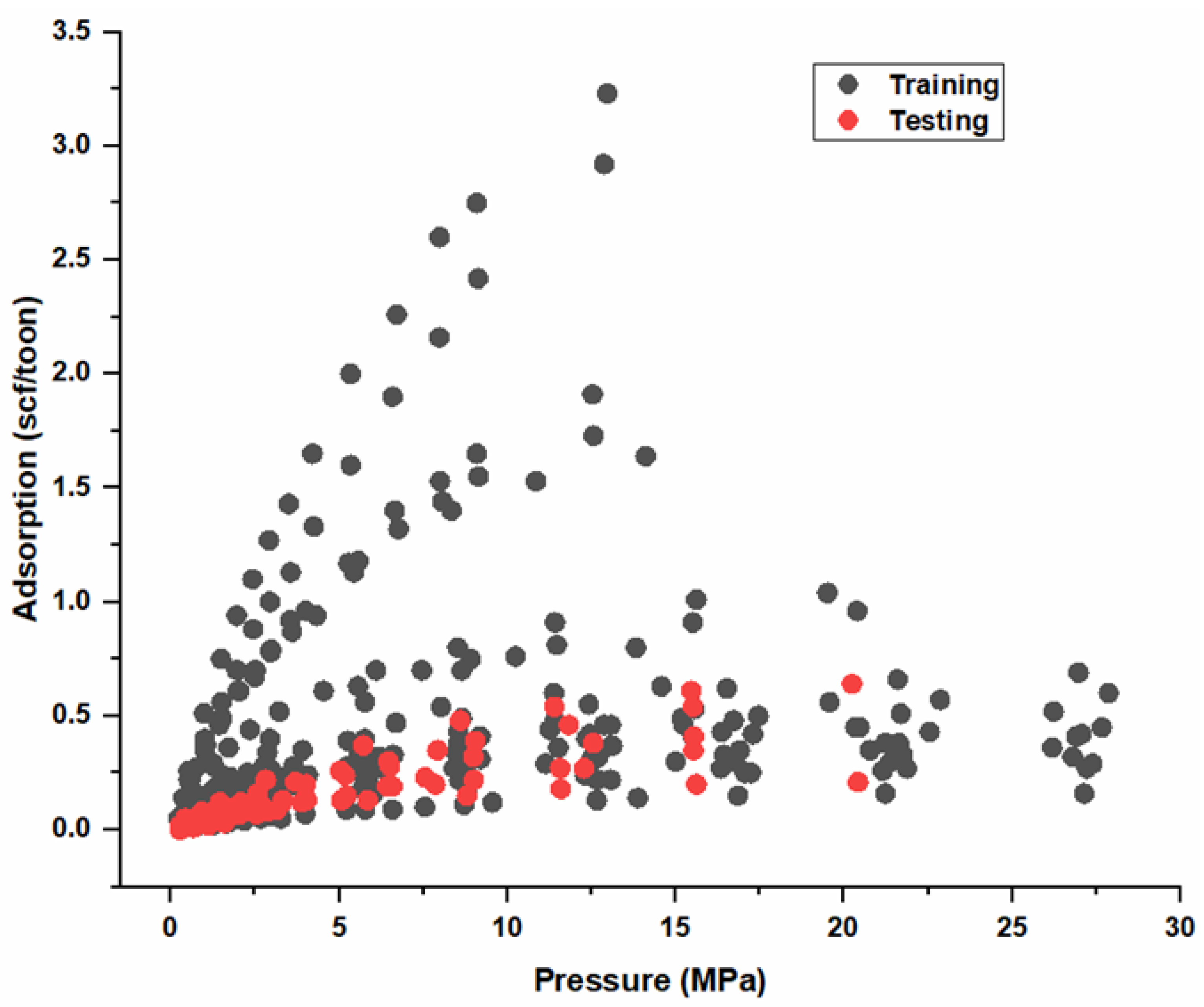
3.1.2. Data Preprocessing

ML algorithms require data in a consistent and interpretable format. Normalization scales features to a standard range (e.g., 0 to 1) to prevent variables with larger scales from dominating the model training. Train–test splitting ensures that the model’s performance is assessed on unseen data, helping evaluate generalization. An 80/20 split is commonly used to maintain a balance between training accuracy and validation integrity.
Normalization:
[ X norm = X X m i n X m a x X m i n ]
Train test Split: 80% training, 20% testing (randomized to avoid bias).

3.1.3. Machine Learning Models

  • XGBoost Model:
XGBoost is a gradient boosting framework that builds trees sequentially, where each new tree attempts to correct the errors of the previous ones. It uses second-order derivatives to optimize the objective function more efficiently. It is particularly suited for tabular data with strong predictive power and offers mechanisms like regularization to prevent overfitting. The loss function, Mean Squared Error (MSE), is minimized during training to ensure accurate regression outcomes.
Objective Function:
[ L ϕ = i = 1 n l y i , y i ^ + k = 1 K Ω f k ] ( Ω f k = γ T + 1 2 λ | w | 2 )   ( r e g u l a r i z a t i o n )
Loss function: ( l y i , y i ^ ) :   MSE.
Prediction:
y i ^ = k = 1 K f k x i , f k F   ( ensemble   of   trees )
  • ANN Model:
ANNs mimic the information processing of biological neurons. An input layer receives features (TOC, temperature, pressure, moisture), while hidden layers perform nonlinear transformations using activation functions like ReLU. The output layer produces the final prediction. Training involves adjusting weights to minimize a loss function, which in this case is MSE, that measures prediction error. ANNs are powerful for capturing complex nonlinear relationships that traditional regression may miss.
Architecture:
-
Input layer: 4 neurons (TOC, T, P, M).
-
Hidden layers: (28, 50) neurons (ABC) or (41, 88) neurons (PSO).
-
Output layer: 1 neuron (MSC).
-
Activation: ReLU for hidden layers, linear for output.
-
Loss Function: MSE.
Optimization:
-
PSO: Updates weights by minimizing MSE via particle swarm dynamics.
-
ABC: Adjusts weights using bee colony foraging behavior.

3.1.4. Optimization Algorithms

  • Particle Swarm Optimization (PSO):
PSO is a population-based stochastic optimization technique inspired by the social behavior of birds. Each particle represents a candidate solution and adjusts its velocity and position in the solution space based on personal experience and the global best solution. This algorithm is effective for tuning neural network weights and hyperparameters due to its simplicity and convergence capability.
Velocity Update:
[ v i t + 1 = w v i t + c 1 r 1 p best x i t + c 2 r 2 g best x i t ]
Position Update:
[ x i t + 1 = x i t + v i t + 1 ]
-
(w): Inertia weight; (c1, c2): Learning factors; (r1, r2): Random numbers.
Details on the velocity and position updates in PSO are provided in Section 3.2.1 and Section 3.2.2, respectively.
  • Artificial Bee Colony (ABC)
ABC simulates the intelligent foraging behavior of honeybees. Employed bees search for food (solutions), onlooker bees choose food sources based on their profitability (fitness), and scout bees randomly explore new areas. The balance between exploration and exploitation makes ABC well suited for optimizing complex nonlinear functions like those in ML training processes.
Employed Bees: Explore solutions via
[ x new = x i + ϕ i x i x k ]
( ϕ i ) : Random number in [−1, 1].
Onlooker Bees: Select solutions probabilistically based on fitness.

3.1.5. Performance Metrics

-
R2 (Coefficient of Determination):
R 2 = 1 y i y i ^ 2 y i y ¯ 2 ]
-
RMSE (Root Mean Squared Error):
RMSE = 1 n i = 1 n y i y i ^ 2 ]

3.2. Hyperparameter Optimization

To evaluate the optimization performance of ANN and XGBoost models with PSO and ABC algorithms, a standard ML optimization workflow was employed. The following section describes the steps used for the ANN and XGBoost hyperparameter optimization process using PSO and ABC algorithms.

3.2.1. Optimization of ANN with PSO and ABC

The flowchart in Figure 3 describes the ANN hyperparameter optimization process using PSO and ABC algorithms. The objective was to identify the best ANN configuration by iteratively refining hyperparameters using SI and foraging-based optimization until convergence is achieved. The optimization process for ANN consisted of the following steps: The dataset was first imported, cleaned, and normalized using Min-Max scaling to ensure uniformity in feature ranges. The ANN model was designed to predict MSC based on four input features: TOC, temperature, pressure, and moisture, represented by four neurons in the input layer. Two hidden layers were incorporated, with the ANN-ABC model utilizing 28 and 50 neurons, while the ANN-PSO model employed 41 and 88 neurons, respectively. The ReLU activation function was applied in the hidden layers to introduce nonlinearity, and a linear activation function was used in the output layer, which consisted of a single neuron corresponding to the MSC. Model training was guided by the MSE as the loss function, ensuring accurate minimization of prediction errors.
The PSO algorithm was configured with a swarm size of 30 particles and a maximum of 100 iterations to optimize the ANN parameters. Each particle in the swarm represented a potential ANN configuration, including hidden layer sizes and learning rate. The inertia weight (w) was set to 0.7 to balance exploration and exploitation, while the cognitive and social acceleration coefficients were both defined as c1, c2 = 1.5. At each iteration, random coefficients r1, r2 ∈ [0, 1] were independently sampled from a uniform distribution in the range [0, 1].
Particle velocities and positions were then updated using the standard PSO velocity and position update Equations (4) and (5), allowing the swarm to iteratively search for an optimal solution.
The ABC algorithm was implemented with a colony size of 30 bees, equally divided into 10 employed bees, 10 onlooker bees, and 10 scout bees. An abandonment limit of 50 cycles was set, meaning that if a solution did not improve after 50 iterations, it was abandoned, and a scout bee was activated to explore a new random solution. Employed bees were responsible for exploring food sources in the neighborhood of their current positions (see Equation (6)), while onlooker bees selected food sources based on a probability proportional to their fitness values, thus favoring better solutions. When solutions stagnated, scout bees introduced diversity by generating new random candidate solutions, helping the algorithm escape local optima and maintain global search capability.
The optimization process was terminated either when the MSE reached a predefined minimal threshold (convergence) or when the maximum number of iterations was completed. The best-performing ANN configuration from either PSO or ABC optimization was selected for final model training and evaluation
A summary of the optimized ANN hyperparameters is shown in Table 1. These settings demonstrated superior predictive performance and generalization ability of methane sorption capacity prediction in heterogeneous porous media.

3.2.2. Optimization of XGBoost with PSO and ABC

The flowchart in Figure 4 outlines the hyperparameter tuning process for the XGBoost model using the particle swarm optimization (PSO) and artificial bee colony (ABC) algorithms. These metaheuristic methods were applied to efficiently explore the hyperparameter space and optimize model performance by minimizing prediction errors. The optimization process included the following steps: The dataset was first imported, cleaned, and normalized using Min-Max scaling to ensure consistent feature scaling. It was then formatted into XGBoost’s optimized DMatrix structure to enable efficient computation and memory handling during training. To begin the model optimization process, initial hyperparameter ranges were defined according to the following key parameters: max_depth, which controls the maximum depth of individual trees; n_estimators, representing the total number of boosting rounds; and learning_rate, a step-size shrinkage factor used to prevent overfitting and enhance model generalization.
PSO algorithm was employed to optimize the hyperparameters of the XGBoost model. The swarm consisted of 30 particles and was iterated over a maximum of 100 cycles. An inertia weight (w) of 0.7 was used to balance exploration and exploitation, while the cognitive and social acceleration coefficients (c1 = 1.5, c2 = 1.5) guided the particles toward personal and global best solutions. Each particle in the swarm encoded a unique combination of XGBoost hyperparameters, including max_depth, n_estimators, and learning_rate. The fitness of each particle was evaluated using 5-fold cross-validation, with Root Mean Squared Error (RMSE) serving as the performance metric. During each iteration, random coefficients r1, r2 were drawn from a uniform distribution in the range [0, 1], and the particles’ velocities and positions were updated accordingly using standard PSO Equations (4) and (5).
The ABC algorithm was applied to optimize XGBoost hyperparameters, using a colony of 30 bees divided equally into 10 employed, 10 onlooker, and 10 scout bees. The optimization process was carried out over a maximum of 100 cycles. Each food source in the colony represented a distinct set of XGBoost hyperparameters (e.g., max_depth, n_estimators, learning_rate). Employed bees explored neighboring solutions around their current food sources to find improved configurations. Onlooker bees evaluated the fitness of these food sources and probabilistically selected among them based on their performance. If a food source failed to improve after 50 consecutive cycles, it was abandoned, and scout bees were activated to explore entirely new random solutions, thereby maintaining diversity and avoiding local optima.
RMSE was used as the performance metric, with fitness calculated via 5-fold cross-validation. The optimization process terminated upon reaching convergence criteria (minimum RMSE or 100 iterations). The best-performing hyperparameter set was selected and reported in Table 1. This detailed optimization protocol ensures robust model calibration and enhances the predictive capability of XGBoost for methane sorption capacity prediction in heterogeneous porous media.

3.3. Model Calibration, Validation, and Performance Evaluation

To achieve accurate predictions of MSC in shale, the optimization of ANN and XGBoost models with PSO and ABC is performed using a training set comprising 80% of data samples. The remaining 20% of data samples are designated for testing. The separation of the training and testing sets from the entire dataset is depicted in Figure 5. To prevent data bias, the training and testing sets are located throughout the entire dataset [37]. Each data sample consists of five input variables (pressure, temperature, TOC, and moisture) and one output variable, MSC. To ensure consistency, the adsorption data with different units are standardized. It is also worth mentioning that the training data span a larger range than the test data, which is due to random sample bias; the training set was disproportionately allocated extreme values. To counter this, we made sure that the distributions of the three main variables (temperature, pressure, and TOC) were comparable in both sets. Additionally, the parameter space may not be fully captured by the small test samples (20% of 352 data points). While the 80:20 random train–test split is commonly used, it may not adequately capture the full distribution of the data, particularly at the extremes. We observed that the test set contained fewer high or low values for critical variables such as temperature and TOC, which could introduce biases in model evaluation. Although we ensured similar distributions between sets through randomization, no formal stratification technique was applied. In future work, we recommend employing stratified sampling or implementing k-fold cross-validation to improve generalization assessment and reduce potential biases caused by unbalanced test subsets.
Furthermore, for consistency of data preprocessing to avoid fabricated disparities, test data were normalized using scaling parameters from the training set. Despite these differences, the model achieves high accuracy (R2 > 0.99 for ANN-PSO), suggesting effective generalization.
The optimization outcomes of these four techniques employing Beaton’s data are displayed in Figure 6. Each graphic displays the projected adsorption on the y-axis and the experimental adsorption on the x-axis. The red line is the 100% agreement line, and the points are optimized results. The ML algorithm’s prediction accuracy increases with the points’ proximity to the red line. Table 2 presents the findings of evaluation metrics to compare various ML algorithms’ performance quantitatively. By comparison, the current work’s ANN-ABC and ANN-PSO models outperform all previous studies, with higher R2 values (0.9913 and 0.9954) and lower RMSE scores (0.0457 and 0.0420), respectively, indicating improved predictive accuracy and generalization ability (Table 2) [22,36,38,54,55]. The performance of the trained ANN-ABC and ANN-PSO models are shown in Figure 7, and the predictions are highly similar to experiments. Compared to XGBoost Meng [22] (R2 = 0.9781, RMSE = 0.0053), the ANN-based models in the current study perform better. Compared to CatBoost Mao, 2023 [55] (R2 = 0.986, RMSE = 0.022), ANN-ABC and ANN-PSO further enhance predictive efficiency. The hybrid models (XGBoost-ABC and XGBoost-PSO) in the current study show lower performance compared to ANN-based models, with XGBoost-PSO performing the worst (R2 = 0.6738, RMSE = 0.0922). Hybrid XGBoost models underperform, likely due to the incompatibility of boosting algorithms with these optimization techniques. Furthermore, by utilizing distributed representations through hidden layers, ANNs improve generalization in complicated datasets in contrast to XGBoost, which depends on sequential decision trees [56]. For the best results, XGBoost needs human feature engineering or preprocessing (e.g., addressing missing values, scaling). On the other hand, ANNs eliminate reliance on domain expertise by automatically learning hierarchical features through backpropagation [57].

3.4. Comparison of Proposed ML Model with Previous Model

ML models have significantly advanced the accuracy and efficiency of predicting MSC in shale formations. In high-dimensional and non-convex search spaces, conventional gradient-based optimization techniques (such as SGD and Adam) and even some metaheuristics, such as genetic algorithms (GAs), frequently converge too soon to less-than-ideal solutions [58]. Because PSO and ABC are swarm intelligence-based algorithms, they keep track of a population of potential solutions, which makes searching more globally possible and lowers the possibility of becoming trapped in local optima [59].
Hyperparameters (such as learning rate and kernel parameters) are used by ML models like XGBoost and GPR; however, they do not always produce differentiable loss landscapes. PSO and ABC are more robust for discontinuous and noisy optimization tasks because they do not require gradient information, in contrast to gradient-based techniques (e.g., Bayesian optimization using Gaussian processes) [60].
As mentioned above, ANN performed better in this study than XGBoost; therefore, in this section, we will discuss the implications of ANN-PSO and ANN-ABC in the context of MSC prediction in shale. Various models have been explored by researchers, each with their own strengths and limitations (Table 3). The present work introduces an advanced hybrid approach using ANN combined with SI techniques, specifically ABC and PSO. Below, we discussed how the current proposed model strengthens the methane prediction in heterogeneous porous material in terms of learning approach, model complexity, performance comparison, prediction accuracy, computational efficiency, and model optimization as compared to other models mentioned in Table 3.

3.4.1. Learning Approach and Model Complexity

Traditional ensemble learning models (XGBoost, CatBoost) are tree-based ensemble models that use boosting strategies to improve accuracy and reduce bias [22,55]. These models excel at handling structured data and have demonstrated high accuracy in shale gas adsorption predictions. However, they may struggle with capturing highly nonlinear relationships in adsorption behavior, especially under complex reservoir conditions. Probabilistic and regression models such as GPR provide uncertainty estimates, making them suitable for predictions with limited datasets. The performance of the model is optimized by another PSO-SVR. Though they may need to be adjusted for huge datasets, these models are good at striking a balance between accuracy and computing efficiency. Models of optimization are inspired by biology in order to represent intricate adsorption interactions. GEP (gene expression programming) imitates how neurons function, whereas GWO-SVM uses an optimization technique inspired by nature to emulate hierarchical hunting behavior. These models are more accurate, but because they are iterative, they could take longer to train.
This study’s methodology combines ANN with bio-inspired optimization methods like ABC and PSO. By optimizing the ANN’s weight modifications, the SI approaches decrease training time and increase accuracy. By effectively capturing intricate adsorption dynamics while preserving computing efficiency, our hybrid technique overcomes the drawbacks of conventional ML models.

3.4.2. Performance Comparison and Prediction Accuracy

High prediction accuracy is offered by XGBoost and CatBoost, which beat traditional regression models. They are not, however, flexible in adsorption circumstances with extreme changes. Although GPR and PSO-SVR models increase computing efficiency, they might not be able to handle large-scale shale gas datasets. Bio-inspired improvements are introduced by GWO-SVM and GEP, improving adsorption predictions but demanding more processing power. By merging deep learning and SI, this work (ANN-ABC, ANN-PSO) provides greater accuracy in forecasting MSC, enabling better management of nonlinear adsorption properties.

3.4.3. Computational Efficiency and Accuracy

In this study, the ANN-PSO model outperforms GPR or GWO-SVM because the ANN-PSO hybrid blends the global search efficiency of PSO [58] with the universal approximation power of ANNs. This enables it to better capture complex, nonlinear patterns than GWO-SVM, whose performance is kernel-dependent [46], and Gaussian Process Regression (GPR), which depends on preset kernel functions [61].
By examining the weight space globally, PSO lessens the ANN’s propensity to converge to local minima [62]. GPR, on the other hand, uses marginal likelihood maximization to optimize hyperparameters, which can be computationally demanding and less than ideal for high-dimensional data [63]. Although GWO-SVM enhances SVM’s hyperparameters (such as CC and γγ), it is still limited by the kernel’s intrinsic features [64].
According to J. Quinonero-Candela [65], ANN-PSO scales are better than GPR, which has O(n3) complexity as a result of covariance matrix inversions. Compared to grid-search SVM, GWO-SVM lowers computing costs, but it still has problems with big datasets [66]. Large-scale, noisy applications can benefit from ANN-PSO’s parallelizable training and PSO’s effective search [67].

4. Conclusions

In this study, two robust intelligent approaches, namely ANN with bio-inspired optimization techniques and the traditional ensemble learning model XGBoost, were applied to predict MSC in heterogeneous porous material, i.e., shale gas formations. A databank comprising five parameters, including temperature, pressure, moisture, TOC, and MSC, and consisting of 352 data points, was assembled from the literature. The models’ goal was to estimate MSC as the target variable, and the first four parameters were entered as input parameters. Models were trained and correlations were created using 80% of the databank; the remaining data were taken into consideration to verify the validity and accuracy of the correlations that were created. Various graphical and statistical evaluations were used to make sure the generated correlations produced reliable and consistent predictions. The following are the main findings of this study:
  • Hybrid XGBoost models underperform, likely due to the incompatibility of boosting algorithms with ABC and PSO optimization techniques.
  • The hybrid ANN-ABC and ANN-PSO models in this study outperform traditional ML models by enhancing prediction accuracy through SI optimization and improving adaptability to diverse shale gas reservoir conditions.
  • This study offers a reliable numerical modeling framework for predicting methane sorption in heterogeneous shale formations by integrating XGBoost and ANN optimized by PSO and ABC. The models efficiently capture nonlinear interactions among geochemical and thermodynamic factors, giving greater accuracy for gas-in-place predictions in shale gas reservoirs.
  • The findings in this work represent an advanced approach to MSC prediction, leveraging the strengths of deep learning and SI for improved accuracy, efficiency, and scalability.
  • The petroleum industry can utilize this model in commercial software to predict the amount of producible gas in shale reservoirs and make it easier for these reservoirs to operate.
Despite the promising performance of the proposed ML models, several limitations should be acknowledged. First, the dataset size (N = 352) is relatively small, which may limit the generalizability of the models to broader geological settings. Second, the data were primarily sourced from Beaton [39,40], focusing on shale formations in a specific geographic region. This geographic specificity may introduce biases and reduce the model’s applicability to other shale systems with different geological contexts. Third, key variables such as mineralogical composition, pore structure, and specific surface area were not included due to data unavailability. These factors can significantly influence methane adsorption behavior and should be incorporated into future studies to enhance model accuracy and generalization.

Author Contributions

Conceptualization, T.I. and S.M.I.; methodology, T.I.; software, T.I. and R.J.; validation, T.I. and S.M.I.; formal analysis, T.I. and S.M.I.; investigation, T.I. and R.J.; resources, S.M.I.; data curation, R.J.; writing—original draft preparation, T.I. and S.M.I.; writing—review and editing, S.M.I.; visualization, H.T.; supervision, S.M.I.; project administration, S.M.I. All authors have read and agreed to the published version of the manuscript.

Funding

This research received no external funding.

Institutional Review Board Statement

Not applicable.

Informed Consent Statement

Not applicable.

Data Availability Statement

The original contributions presented in this study are included in the article. Further inquiries can be directed to the corresponding author.

Conflicts of Interest

The authors declare no conflicts of interest.

Abbreviations

The following abbreviations are used in this manuscript:
XGBoostExtreme gradient boosting
ANNArtificial neural network
ABCArtificial bee colony
PSOParticle swarm optimization
GPRGaussian Process Regression
GEPGene expression programming
GWOGray wolf optimizer
SVMSupport vector machine
SVRSupport vector regression
SSASparrow search algorithm
GIPGas-in-place
MSCMethane sorption capacity
MLMachine learning
TOCTotal organic carbon
SISwarm intelligence

References

  1. Zhang, W.; Chen, W.; Wang, T.; Yuan, Y. A self-similarity mathematical model of carbon isotopic flow fractionation during shale gas desorption. Phys. Fluids 2019, 31, 112005. [Google Scholar]
  2. Gu, J.; Liu, G.; Gao, F.; Hu, Y.; Ye, D. Multiple seepage model and gas production simulation of shale with power law fracture distribution. Phys. Fluids 2023, 35, 11. [Google Scholar]
  3. Middleton, R.S.; Gupta, R.; Hyman, J.D.; Viswanathan, H.S. The shale gas revolution: Barriers, sustainability, and emerging opportunities. Appl. Energy 2017, 199, 88–95. [Google Scholar]
  4. Huang, H.; Sun, W.; Xiong, F.; Chen, L.; Li, X.; Gao, T.; Jiang, Z.; Ji, W.; Wu, Y.; Han, J. A novel method to estimate subsurface shale gas capacities. Fuel 2018, 232, 341–350. [Google Scholar]
  5. Huang, H.; Li, R.; Jiang, Z.; Li, J.; Chen, L. Investigation of variation in shale gas adsorption capacity with burial depth: Insights from the adsorption potential theory. J. Nat. Gas Sci. Eng. 2020, 73, 103043. [Google Scholar]
  6. Tang, X.; Ripepi, N.; Stadie, N.P.; Yu, L.; Hall, M.R. A dual-site Langmuir equation for accurate estimation of high pressure deep shale gas resources. Fuel 2016, 185, 10–17. [Google Scholar]
  7. Fan, L.; Liu, S. A novel experimental system for accurate gas sorption and its application to various shale rocks. Chem. Eng. Res. Des. 2021, 165, 180–191. [Google Scholar]
  8. Middleton, R.S.; Carey, J.W.; Currier, R.P.; Hyman, J.D.; Kang, Q.; Karra, S.; Jiménez-Martínez, J.; Porter, M.L.; Viswanathan, H.S. Shale gas and non-aqueous fracturing fluids: Opportunities and challenges for supercritical CO2. Appl. Energy 2015, 147, 500–509. [Google Scholar]
  9. International Energy Agency (IEA). World Energy Outlook 2022; International Energy Agency (IEA): Paris, France, 2022. [Google Scholar]
  10. Tang, H.; Yu, Y.; Sun, Q. Progress, Challenges, and Strategies for China’s Natural Gas Industry Under Carbon-Neutrality Goals. Processes 2024, 12, 1683. [Google Scholar]
  11. Rivard, C.; Lavoie, D.; Lefebvre, R.; Séjourné, S.; Lamontagne, C.; Duchesne, M. An overview of Canadian shale gas production and environmental concerns. Int. J. Coal Geol. 2014, 126, 64–76. [Google Scholar]
  12. Wang, Q.; Li, R. Research status of shale gas: A review. Renew. Sustain. Energy Rev. 2017, 74, 715–720. [Google Scholar]
  13. Hays, J.; Finkel, M.L.; Depledge, M.; Law, A.; Shonkoff, S.B.C. Considerations for the development of shale gas in the United Kingdom. Sci. Total Environ. 2015, 512, 36–42. [Google Scholar]
  14. Negi, B.S.; Pandey, K.K.; Sehgal, N. Renewables, shale gas and gas import-striking a balance for India. Energy Procedia 2017, 105, 3720–3726. [Google Scholar]
  15. Costa, D.; Neto, B.; Danko, A.S.; Fiúza, A. Life Cycle Assessment of a shale gas exploration and exploitation project in the province of Burgos, Spain. Sci. Total Environ. 2018, 645, 130–145. [Google Scholar]
  16. Ibad, S.M.; Padmanabhan, E. Methane sorption capacities and geochemical characterization of Paleozoic shale Formations from Western Peninsula Malaysia: Implication of shale gas potential. Int. J. Coal Geol. 2020, 224, 103480. [Google Scholar] [CrossRef]
  17. Ibad, S.M.; Padmanabhan, E. Inorganic geochemical, mineralogical and methane sorption capacities of Paleozoic shale formations from Western Peninsular Malaysia: Implication of shale gas potential. Appl. Geochem. 2022, 140, 105269. [Google Scholar] [CrossRef]
  18. Davenport, J.; Wayth, N. Statistical Review of World Energy; Energy Institute: London, UK, 2023. [Google Scholar]
  19. Lin, X.; Liu, C.; Wang, Z. The influencing factors of gas adsorption behaviors in shale gas reservoirs. Front. Earth Sci. 2023, 10, 1021983. [Google Scholar]
  20. Hu, K.; Zhang, Q.; Liu, Y.; Thaika, M.A. A developed dual-site Langmuir model to represent the high-pressure methane adsorption and thermodynamic parameters in shale. Int. J. Coal Sci. Technol. 2023, 10, 59. [Google Scholar]
  21. Chen, L.; Zuo, L.; Jiang, Z.; Jiang, S.; Liu, K.; Tan, J.; Zhang, L. Mechanisms of shale gas adsorption: Evidence from thermodynamics and kinetics study of methane adsorption on shale. Chem. Eng. J. 2019, 361, 559–570. [Google Scholar]
  22. Meng, M.; Zhong, R.; Wei, Z. Prediction of methane adsorption in shale: Classical models and machine learning based models. Fuel 2020, 278, 118358. [Google Scholar] [CrossRef]
  23. Jiang, Z.; Zhao, L.; Zhang, D. Study of adsorption behavior in shale reservoirs under high pressure. J. Nat. Gas. Sci. Eng. 2018, 49, 275–285. [Google Scholar]
  24. Curtis, J.B. Fractured shale-gas systems. Am. Assoc. Pet. Geol. Bull. 2002, 86, 1921–1938. [Google Scholar]
  25. Li, Q.; Li, Q.; Cao, H.; Wu, J.; Wang, F.; Wang, Y. The Crack Propagation Behaviour of CO2 Fracturing Fluid in Unconventional Low Permeability Reservoirs: Factor Analysis and Mechanism Revelation. Processes 2025, 13, 159. [Google Scholar] [CrossRef]
  26. Yang, Y.; Liu, S. Review of shale gas sorption and its models. Energy Fuels 2020, 34, 15502–15524. [Google Scholar]
  27. Razavi, R.; Bemani, A.; Baghban, A.; Mohammadi, A.H.; Habibzadeh, S. An insight into the estimation of fatty acid methyl ester based biodiesel properties using a LSSVM model. Fuel 2019, 243, 133–141. [Google Scholar]
  28. Dashti, A.; Raji, M.; Alivand, M.S.; Mohammadi, A.H. Estimation of CO2 equilibrium absorption in aqueous solutions of commonly used amines using different computational schemes. Fuel 2020, 264, 116616. [Google Scholar]
  29. Daneshfar, R.; Bemani, A.; Hadipoor, M.; Sharifpur, M.; Ali, H.M.; Mahariq, I.; Abdeljawad, T. Estimating the heat capacity of non-Newtonian ionanofluid systems using ANN, ANFIS, and SGB tree algorithms. Appl. Sci. 2020, 10, 6432. [Google Scholar]
  30. Nabipour, N.; Daneshfar, R.; Rezvanjou, O.; Mohammadi-Khanaposhtani, M.; Baghban, A.; Xiong, Q.; Li, L.K.; Habibzadeh, S.; Doranehgard, M.H. Estimating Biofuel Density Via a Soft Computing Approach Based Intermolecular interactions. Renew. Energy 2020, 152, 1086–1098. [Google Scholar]
  31. Karkevandi-Talkhooncheh, A.; Rostami, A.; Hemmati-Sarapardeh, A.; Ahmadi, M.; Husein, M.M.; Dabir, B. Modeling minimum miscibility pressure during pure and impure CO2 flooding using hybrid of radial basis function neural network and evolutionary techniques. Fuel 2018, 220, 270–282. [Google Scholar]
  32. Rostami, A.; Hemmati-Sarapardeh, A.; Shamshirband, S. Rigorous prognostication of natural gas viscosity: Smart modeling and comparative study. Fuel 2018, 222, 766–778. [Google Scholar]
  33. Daneshfar, R.; Keivanimehr, F.; Mohammadi-Khanaposhtani, M.; Baghban, A. A neural computing strategy to estimate dew-point pressure of gas condensate reservoirs. Pet. Sci. Technol. 2020, 38, 706–712. [Google Scholar]
  34. Vanani, M.B.; Daneshfar, R.; Khodapanah, E. A novel MLP approach for estimating asphaltene content of crude oil. Pet. Sci. Technol. 2019, 37, 2238–2245. [Google Scholar]
  35. Najafi-Marghmaleki, A.; Tatar, A.; Barati-Harooni, A.; Arabloo, M.; Rafiee-Taghanaki, S.; Mohammadi, A.H. Reliable modeling of constant volume depletion (CVD) behaviors in gas condensate reservoirs. Fuel 2018, 231, 146–156. [Google Scholar]
  36. Syah, R.; Naeem, M.H.T.; Daneshfar, R.; Dehdar, H.; Soulgani, B.S. On the prediction of methane adsorption in shale using grey wolf optimizer support vector machine approach. Petroleum 2022, 8, 264–269. [Google Scholar] [CrossRef]
  37. Zhou, Y.; Hui, B.; Shi, J.; Shi, H.; Jing, D. Machine learning method for shale gas adsorption capacity prediction and key influencing factors evaluation. Phys. Fluids 2024, 36, 016604. [Google Scholar]
  38. Chinamo, D.S.; Bian, X.; Liu, Z.; Cheng, J.; Huang, L. Estimation of Adsorption Gas in Shale Gas Reservoir by Using Machine Learning Methods. SSRN 4885195. 2024. Available online: https://www.ijfmr.com/papers/2024/5/27082.pdf (accessed on 16 April 2025).
  39. Beaton, A.P.; Pawlowicz, J.G.; Anderson, S.D.A.; Berhane, H.; Rokosh, C.D. Rock eval, total organic carbon and adsorption isotherms of the Duvernay and Muskwa formations in Alberta: Shale gas data release. Energy Resour. Conserv. Board. 2010, 4, 33. [Google Scholar]
  40. Beaton, A.P.; Pawlowicz, J.G.; Anderson, S.D.A.; Rokosh, C.D. Rock eval, total organic carbon, isotherms and organic petrography of the Colorado Group: Shale gas data release. Energy Resour. Conserv. Board. 2008, 11, 88. [Google Scholar]
  41. Brownlee, J. XGBoost with Python: Gradient Boosted Trees with XGBoost and Scikit-Learn; Machine Learning Mastery: San Juan, Puerto Rico, 2016. [Google Scholar]
  42. Chen, T.; Guestrin, C. Xgboost: A scalable tree boosting system. In Proceedings of the 22nd ACM SIGKDD International Conference on Knowledge Discovery and Data Mining, San Francisco, CA, USA, 13–17 August 2016; pp. 785–794. [Google Scholar]
  43. Bemani, A.; Baghban, A.; Mohammadi, A.H.; Andersen, P.Ø. Estimation of adsorption capacity of CO2, CH4, their binary mixtures in Quidam shale using LSSVM: Application in CO2 enhanced shale gas recovery CO2 storage. J. Nat. Gas Sci. Eng. 2020, 76, 103204. [Google Scholar] [CrossRef]
  44. Vapnik, V. The Nature of Statistical Learning Theory; Springer Science & Business Media: Berlin/Heidelberg, Germany, 2013. [Google Scholar]
  45. Raji, M.; Dashti, A.; Alivand, M.S.; Asghari, M. Novel prosperous computational estimations for greenhouse gas adsorptive control by zeolites using machine learning methods. J. Environ. Manag. 2022, 307, 114478. [Google Scholar] [CrossRef]
  46. Mirjalili, S.; Mirjalili, S.M.; Lewis, A.; Optimizer, G.W. Advances in engineering software. Renew. Sustain. Energy Rev. 2014, 69, 46–61. [Google Scholar]
  47. Najari, S.; Gróf, G.; Saeidi, S.; Gallucci, F. Modeling and optimization of hydrogenation of CO2: Estimation of kinetic parameters via Artificial Bee Colony (ABC) and Differential Evolution (DE) algorithms. Int. J. Hydrogen Energy 2019, 44, 4630–4649. [Google Scholar] [CrossRef]
  48. Meng, M.; Qiu, Z.; Zhong, R.; Liu, Z.; Liu, Y.; Chen, P. Adsorption characteristics of supercritical CO2/CH4 on different types of coal a machine learning approach. Chem. Eng. J. 2019, 368, 847–864. [Google Scholar] [CrossRef]
  49. Karaboga, D. An Idea Based on Honey Bee Swarm for Numerical Optimization. Technical Report-tr06. 2005. Available online: https://abc.erciyes.edu.tr/pub/tr06_2005.pdf (accessed on 14 April 2025).
  50. Karaboga, D.; Basturk, B. On the performance of artificial bee colony (ABC) algorithm. Appl. Soft Comput. 2008, 8, 687–697. [Google Scholar]
  51. Panigrahi, B.K.; Shi, Y.; Lim, M.-H. Handbook of Swarm Intelligence: Concepts, Principles and Applications; Springer Science & Business Media: Berlin/Heidelberg, Germany, 2011; Volume 8. [Google Scholar]
  52. Onwunalu, J.E.; Durlofsky, L.J. Application of a particle swarm optimization algorithm for determining optimum well location and type. Comput. Geosci. 2010, 14, 183–198. [Google Scholar]
  53. Sharma, A.; Onwubolu, G. Hybrid particle swarm optimization and GMDH system. In Hybrid Self-Organizing Modeling Systems; Springer: Berlin/Heidelberg, Germany, 2009; pp. 193–231. [Google Scholar]
  54. Amar, M.N.; Larestani, A.; Lv, Q.; Zhou, T.; Hemmati-Sarapardeh, A. Modeling of methane adsorption capacity in shale gas formations using white-box supervised machine learning techniques. J. Pet. Sci. Eng. 2022, 208, 109226. [Google Scholar]
  55. Mao, F. Research on Influencing Factors and Prediction Methods of Shale Gas Content Based on Machine Learning Algorithm. Open Access Libr. J. 2023, 10, 1–16. [Google Scholar] [CrossRef]
  56. Goodfellow, I.; Bengio, Y.; Courville, A.; Bengio, Y. Deep Learning; MIT Press: Cambridge, MA, USA, 2016; Volume 1. [Google Scholar]
  57. Bengio, Y.; Courville, A.; Vincent, P. Representation Learning: A Review and New Perspectives. IEEE Trans. Pattern Anal. Mach. Intell. 2013, 35, 1798–1828. [Google Scholar] [CrossRef] [PubMed]
  58. Eberhart, R.; Kennedy, J. A new optimizer using particle swarm theory. In Proceedings of the MHS’95, Sixth International Symposium on Micro Machine and Human Science, Nagoya, Japan, 4–6 October 1995; pp. 39–43. [Google Scholar] [CrossRef]
  59. Karaboga, D.; Basturk, B. A powerful and efficient algorithm for numerical function optimization: Artificial bee colony (ABC) algorithm. J. Glob. Optim. 2007, 39, 459–471. [Google Scholar] [CrossRef]
  60. Poli, R.; Kennedy, J.; Blackwell, T. Particle swarm optimization. Swarm Intell. 2007, 1, 33–57. [Google Scholar] [CrossRef]
  61. Williams, C.K.I.; Rasmussen, C.E. Gaussian Processes for Machine Learning; MIT Press: Cambridge, MA, USA, 2006; Volume 2. [Google Scholar]
  62. Shi, Y.; Eberhart, R. A modified particle swarm optimizer. In Proceedings of the 1998 IEEE International Conference on Evolutionary Computation Proceedings World Congress on Computational Intelligence (Cat. No. 98TH8360), Anchorage, AK, USA, 4–9 May 1998; pp. 69–73. [Google Scholar]
  63. Snelson, E.; Ghahramani, Z. Sparse Gaussian processes using pseudo-inputs. In Proceedings of the 19th International Conference on Neural Information Processing Systems, Vancouver, BC, Canada, 5–8 December 2005; Volume 18. [Google Scholar]
  64. Suykens, J.A.K.; Vandewalle, J. Least squares support vector machine classifiers. Neural Process Lett. 1999, 9, 293–300. [Google Scholar] [CrossRef]
  65. Quinonero-Candela, J.; Rasmussen, C.E. A unifying view of sparse approximate Gaussian process regression. J. Mach. Learn. Res. 2005, 6, 1939–1959. [Google Scholar]
  66. Hsu, C.-W.; Chang, C.-C.; Lin, C.-J. A Practical Guide to Support Vector Classification. 2003. Available online: https://www.csie.ntu.edu.tw/~cjlin/papers/guide/guide.pdf (accessed on 21 April 2025).
  67. Zhang, Y.; Wang, S.; Ji, G. A comprehensive survey on particle swarm optimization algorithm and its applications. Math. Probl. Eng. 2015, 2015, 931256. [Google Scholar] [CrossRef]
Figure 1. A brief summary of the methodology.
Resources 14 00080 g001
Figure 2. Box plot for each parameter: (A) Temperature and Pressure, (B) Adsorption and Moisture, and (C) TOC.
Resources 14 00080 g002
Figure 3. Schematic depiction of ANN-PSO and ANN-ABC.
Resources 14 00080 g003
Figure 4. Schematic depiction of XGBoost-PSO and XGBoost-ABC.
Resources 14 00080 g004
Figure 5. Division of the testing and training sets for ML optimization.
Resources 14 00080 g005
Figure 6. Comparisons between the model results and measured ones: (A) ANN-ABC, (B) ANN-PSO, (C) XGBoost-ABC, and (D) XGBoost-PSO.
Resources 14 00080 g006aResources 14 00080 g006b
Figure 7. Performance of the ANN model with (A) ABC and (B) PSO.
Resources 14 00080 g007
Table 1. Optimized hyperparameters of the ANN and XGBoost algorithm coupled with ABC and PSO.
ModelHyperparameter
ANN with ABCHidden layer sizes = (28, 50); Activation = ReLU (hidden), Linear (output); Learning rate = 0.0354
Colony size = 30 (10 employed, 10 onlooker, 10 scout); Max cycles = 100; Abandonment limit = 50
ANN with PSOHidden layer sizes = (41, 88); Activation = ReLU (hidden), Linear (output); Learning rate = 0.0077
Swarm size = 30; Max iterations = 100; Inertia weight (w) = 0.7; c1 = 1.5, c2 = 1.5
XGBoost with ABCMax depth = 4; n_estimators = 443; Learning rate = 0.0074
Colony size = 30; Max cycles = 100; Abandonment limit = 50
XGBoost with PSOMax depth = 3; n_estimators = 342; Learning rate = 0.0100
Swarm size = 30; Max iterations = 100; Inertia weight (w) = 0.7; c1 = 1.5, c2 = 1.5
Table 2. Comparison of different models with the current model.
StudiesModelR2RMSE
[22]XGBoost0.9780.005
ANN0.9180.300
RF0.9080.060
SVM0.8410.131
[36]GWO-SVM0.9820.050
[37]GPR0.9700.030
[38]PSO-SVR0.9600.099
GWO-SVR0.9520.109
SSA-SVR0.9360.126
XGBoost0.9600.099
[54]GEP0.983
[55]CatBoost0.9860.022
Current workANN-ABC0.9910.045
ANN-PSO0.9950.042
XGBoost-ABC0.9440.146
XGBoost-PSO0.7620.092
Table 3. Summary of different ML models used to predict MSC in shale rocks, along with relevant references.
ML ModelDescriptionKey Input ParametersAccuracy/PerformanceReference
XGBoostEnsemble learning method that improves prediction accuracy by minimizing bias and variance.Total organic carbon (TOC), temperature, pressure, porosity, clay contentHigh accuracy compared to traditional models.[22]
GWO-SVMSI technique that replicates the hierarchical relationships and hunting behavior of gray wolves in the wild.Temperature, pressure, TOC, moisture, and gas contentProvides a better prediction of the adsorbed gas than models that have been suggested before.[36]
GPRProbabilistic model that provides uncertainty estimates in predictions.TOC, moisture, temperature, pressure, gas compositionPredicts adsorption with an error margin < 3%.[37]
PSO-SVRSwarm intelligence (SI) and vector regression to improve prediction accuracy and computational efficiency.Temperature, TOC, vitrinite reflectance, pressure, and volumePSO-SVR model performed better than other models used in this study.[38]
GEPMimics brain neurons to capture complex nonlinear relationships in adsorption data.TOC, porosity, mineral composition, reservoir pressureOutperforms conventional Langmuir models.[54]
CatBoostTree-structure-based integrated learning model that uses the boosting technique.TOC and pore-specific surface areaThe model achieved an accuracy of 98.6% in predicting shale gas content, outperforming conventional prediction methods.[55]
ANN-ABC
ANN-PSO
Improving model performance by leveraging SI and bee colony behavior.TOC, temperature, pressure, moisture content, and gas contentGives an excellent prediction of the adsorbed
gas compared to previously proposed models.
This study
Disclaimer/Publisher’s Note: The statements, opinions and data contained in all publications are solely those of the individual author(s) and contributor(s) and not of MDPI and/or the editor(s). MDPI and/or the editor(s) disclaim responsibility for any injury to people or property resulting from any ideas, methods, instructions or products referred to in the content.

