Article

Biomass Gasification for Waste-to-Energy Conversion: Artificial Intelligence for Generalizable Modeling and Multi-Objective Optimization of Syngas Production

by
Gema Báez-Barrón
1,
Francisco Javier Lopéz-Flores
1,*,
Eusiel Rubio-Castro
2 and
José María Ponce-Ortega
1,*
1
Chemical Engineering Department, Universidad Michoacana de San Nicolás de Hidalgo, Av. Francisco J. Múgica S/N, Ciudad Universitaria, Edificio V1, Morelia 58060, Mexico
2
Chemical and Biological Sciences Department, Universidad Autónoma de Sinaloa, Culiacán 80000, Mexico
*
Authors to whom correspondence should be addressed.
Resources 2025, 14(10), 157; https://doi.org/10.3390/resources14100157 (registering DOI)
Submission received: 14 August 2025 / Revised: 26 September 2025 / Accepted: 5 October 2025 / Published: 8 October 2025

Abstract

Biomass gasification, a key waste-to-energy technology, is a complex thermochemical process with many input variables influencing the yield and quality of syngas. In this study, data-driven machine learning models are developed to capture the nonlinear relationships between feedstock properties, operating conditions, and syngas composition, in order to optimize process performance. Random Forest (RF), CatBoost (Categorical Boosting), and an Artificial Neural Network (ANN) were trained to predict key syngas outputs (syngas composition and syngas yield) from process inputs. The best-performing model (ANN) was then integrated into a multi-objective optimization framework using the open-source Optimization & Machine Learning Toolkit (OMLT) in Pyomo. An optimization problem was formulated with two objectives—maximizing the hydrogen-to-carbon monoxide (H2/CO) ratio and maximizing the syngas yield simultaneously, subject to operational constraints. The trade-off between these competing objectives was resolved by generating a Pareto frontier, which identifies optimal operating points for different priority weightings of syngas quality vs. quantity. To interpret the ML models and validate domain knowledge, SHapley Additive exPlanations (SHAP) were applied, revealing that parameters such as equivalence ratio, steam-to-biomass ratio, feedstock lower heating value, and fixed carbon content significantly influence syngas outputs. Our results highlight a clear trade-off between maximizing hydrogen content and total gas yield and pinpoint optimal conditions for balancing this trade-off. This integrated approach, combining advanced ML predictions, explainability, and rigorous multi-objective optimization, is novel for biomass gasification and provides actionable insights to improve syngas production efficiency, demonstrating the value of data-driven optimization in sustainable waste-to-energy conversion processes.

1. Introduction

Growing global energy demand, driven by industrial development and societal needs, has intensified dependence on fossil fuels, finite resources whose exploitation contributes to climate change [1]. At the same time, inadequate management of municipal solid waste (MSW) exacerbates the environmental crisis: in 2023, 2.3 billion tons of MSW were generated worldwide, and it is estimated that by 2050, this figure will reach 3.8 billion tons if no structural changes are made to its management [2,3]. Considering these challenges, waste-to-energy technologies emerge as a viable alternative that simultaneously addresses energy demand and reduces waste volume. In this context, biomass emerges as a viable renewable resource to produce clean energy. Through thermochemical processes such as gasification, carbonaceous materials can be converted into synthesis gas (syngas), composed mainly of hydrogen (H2), carbon monoxide (CO), and methane (CH4), along with solid by-products. This syngas can be used to generate heat and electricity, providing an effective means of harnessing energy from organic waste. Over the last decade, global syngas production from biomass gasification has increased notably [4], reflecting the growing interest in this technology.
However, at the industrial scale, biomass gasification faces several limitations, particularly regarding process efficiency [5] and variability in raw materials and operating conditions. Concurrently, the application of advanced artificial intelligence techniques in chemical processes has grown remarkably in recent years [6,7], owing to their effectiveness in modeling complex and nonlinear relationships in cases where traditional mechanistic models prove insufficient. Machine learning (ML) has emerged as a powerful tool for optimizing the performance of gasification systems. ML enables the development of highly accurate predictive models from large volumes of data, effectively capturing complex behavioral patterns. These models allow for a precise representation of the gasification process and enable the evaluation of the relative influence of different operating variables on system performance [8].
In recent years, various methodologies have been developed for modeling the gasification process using ML techniques. Artificial neural networks (ANN) have been particularly prominent in this field. For instance, Xiao et al. [9] trained an ANN to predict the characteristics of gasification in a fluidized bed based on experimental data from five typical organic compounds and three simulated MSW samples, achieving acceptable predictions of process behavior. Similarly, Baruah et al. [8] developed an ANN to model biomass gasification in a downdraft fixed-bed gasifier. Likewise, Serrano et al. [10] incorporated various bed materials as input variables in an ANN model for bubbling fluidized bed gasification, improving the accuracy of predictions for both gas composition and yield. More recently, Ascher et al. [5] reported the development of an ANN model with excellent predictive power for biomass and waste gasification processes. Other ML techniques have also proven viable in this context. Elmaz et al. [11] applied four regression methods to predict syngas composition (CO, CO2, CH4, H2) and its gross calorific value, obtaining highly accurate forecasts. Kardani et al. [12] implemented an optimized ensemble model for modeling MSW gasification. Despite these advances, most previous studies have focused on a limited range of biomass types and gasifier configurations, often addressing specific cases such as MSW gasification. This narrow scope limits the generalizability of the models and prevents systematic comparisons between different operating scenarios, as a wide variety of feedstocks, gasifying agents, reactor designs, and bed materials are typically not considered simultaneously.
On the other hand, hybrid approaches that combine ML techniques with mathematical programming have become powerful tools for optimizing complex process systems [13]. Tools such as OMLT (Optimization and Machine Learning Toolbox) [14] (Ceccon et al., 2022), PySCIPOpt-ML [15], and MathOptAI [16] are commonly used to efficiently implement ML–based predictive models within mathematical optimization frameworks. These platforms enable neural network architectures and other ML algorithms to be expressed as mathematical formulations compatible with mixed-integer linear programming (MILP) or nonlinear programming (NLP) solvers. In this regard, these tools have been applied to optimize the flowback water management in shale gas production [17], the dispatch of energy storage systems [18], the process flow diagram of a Gibbs reactor [19], integrated energy systems [20], photovoltaic solar panel production [21], and green urea production [22]. However, its application to optimizing syngas production via biomass gasification remains unexplored, presenting an opportunity to expand the scope of this tool in energy conversion technologies.
Consequently, this study aims to overcome these limitations by developing advanced and broadly generalizable ML models for biomass gasification. This study is the first to couple a state-of-the-art ML surrogate with a multi-objective optimization framework for biomass gasification (see Figure 1). Three advanced ML models, ANN, Random Forest, and CatBoost, are developed and rigorously compared using an extensive and heterogeneous multi-study dataset, with hyperparameter optimization and SHAP (Shapley Additive Explanations) analysis to quantify the influence of key operating variables. The best-performing model is then embedded, through the open-source OMLT, into an ε-constraint multi-objective optimization that simultaneously maximizes the H2/CO ratio and the overall syngas yield. This integrated data-driven strategy surpasses previous works, which typically either optimize a single objective or rely solely on simplified simulations or purely experimental trade-off analyses, and provides a robust framework for enhancing both the efficiency and the sustainability of biomass-gasification systems.

2. Methodology

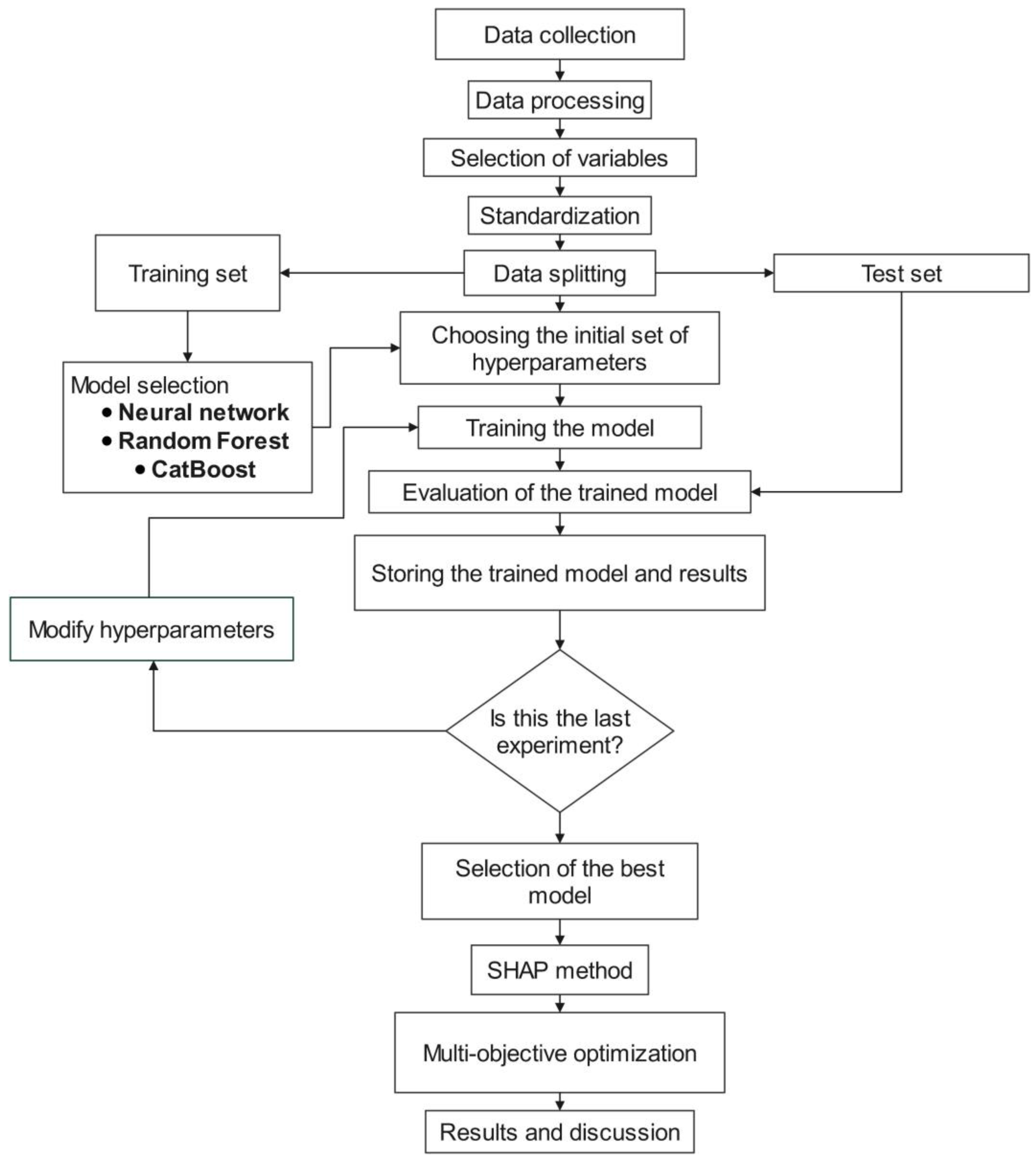
As part of the methodology (see Figure 2), data from experimental trials on biomass gasification are collected and subjected to a selection and preprocessing stage to identify patterns, missing values, and irregularities. In specific cases, missing data are imputed. The most relevant variables are then carefully selected to improve the efficiency and accuracy of the predictive models. Numerical variables are standardized, and categorical variables are transformed using one-hot encoding to make them suitable for ML algorithms. The dataset is divided into training and test sets to ensure robust model evaluation. During the modeling phase, several ML techniques are applied, including ANN, Random Forest, and CatBoost. Hyperparameter optimization is performed to enhance performance and generalization. After training, model accuracy is evaluated using relevant metrics, and the SHAP method is applied to decompose predictions and reveal the impact of individual variables, providing deeper insights into model behavior. Once the best-performing model is identified, multi-objective optimization is conducted to simultaneously maximize H2/CO ratio and syngas yield. Finally, the results are analyzed, and a critical discussion is presented to validate the model and identify potential improvements for future studies.

2.1. Database

To build the ML models, a database of 343 records extracted from 33 published experimental studies was used [23,24,25,26,27,28,29,30,31,32,33,34,35,36,37,38,39,40,41,42,43,44,45,46,47,48,49,50,51,52,53,54,55]. These covered a wide variety of feedstocks (woody biomass, herbaceous biomass, plastics, municipal solid waste, and sewage sludge) and operating conditions, including different conversion agents (air, steam, oxygen, and combinations), reactor configurations (fixed bed and fluidized bed), and bed materials (silica, alumina, among others). The inclusion of categorical data enhanced model accuracy by capturing critical variables such as agent type, reactor type, and bed material.
Table 1 and Table 2 summarize the predictor and target variables in the database, comprising 18 continuous variables and 8 categorical variables. All categorical variables with only two possible values, process operating mode (batch/continuous), system scale (laboratory/pilot), and catalyst use (present/not present), were encoded as binary values (0 or 1, converted to −1 and 1 after normalization). In the current database, all data come from laboratory- or pilot-scale systems; therefore, system scale was coded using this approach.
To ensure proper evaluation, the database was divided into a training set (80%, 272 data points) and a test set (20%, 68 data points). This approach ensured that the models were trained and evaluated appropriately, maximizing their generalization capabilities.

2.2. Machine Learning

ANN are computational frameworks inspired by the brain’s organization and functioning [56]. Their ability to detect intricate, nonlinear patterns makes them especially valuable for tasks such as regression and multi-class classification. An ANN is arranged in several layers of interconnected neurons: each neuron receives input signals, multiplies them by adjustable weights, processes the result through an activation function, and sends the output to the next layer. During training, these weights are iteratively updated, enabling the network to learn from data and generalize effectively. Among the most popular architectures is the Multi-Layer Perceptron (MLP), a fully connected, feed-forward network consisting of input, hidden, and output layers. The number of neurons in the input and output layers typically corresponds to the count of features and target variables, respectively, whereas the depth and width of the hidden layers vary according to problem complexity. Within these hidden layers, neurons apply nonlinear transformations to their weighted inputs, allowing the MLP to capture sophisticated data relationships that elude traditional linear models [57].
Random Forest is an ensemble learning technique that boosts predictive performance by aggregating the results of many decision trees. Each tree is built from a distinct bootstrapped sample of the original dataset, introducing purposeful variety among the individual models. This diversity lowers the overall variance of the ensemble and guards against overfitting. In classification problems, the algorithm outputs the class chosen by the majority of trees, whereas in regression tasks, it reports the mean value predicted across all trees. By merging multiple weak learners, Random Forest grasps intricate, nonlinear relationships more reliably than a single decision tree, which can suffer from instability and excessive complexity [58]. Beyond its predictive strength, the structure of Random Forest naturally yields estimates of feature importance, clarifying how each variable influences the model’s output. Its capacity to manage high-dimensional datasets and suitability for both classification and regression make it a versatile option across many domains. This combination of flexibility, interpretability, and resistance to overfitting proves especially valuable when analyzing data with numerous predictors, offering insight into latent patterns without sacrificing accuracy [59].
CatBoost, short for Categorical Boosting, is a state-of-the-art tree-ensemble method tailored to classification and regression problems that feature many categorical attributes. In contrast to conventional boosting frameworks, CatBoost ingests these categorical fields directly, eliminating the need for one-hot encoding and thereby avoiding the associated surge in dimensionality and training time [60]. Its “ordered boosting” strategy relies on permutation-based splits that curb information leakage, yielding models that generalize better and resist overfitting. Additional refinements, such as automated feature combinations, effective handling of missing values, and built-in regularization, equip CatBoost to excel on large, heterogeneous datasets while maintaining reliable accuracy across a wide spectrum of use cases [61]. Although both CatBoost and Random Forest perform well on limited data, CatBoost’s native treatment of categorical inputs and its ordered boosting mechanism give it a notable advantage in curbing overfitting and producing models that transfer more robustly to unseen data. This benefit becomes especially pronounced when the dataset contains intricate categorical structures yet only a modest number of samples.

2.2.1. Model Evaluation

The performance of ML models is evaluated using key metrics: Correlation Coefficient (R2), Root Mean Square Error (RMSE), Mean Absolute Error (MAE) and Mean Absolute Percentage Error (MAPE). Conceptually, the higher the R2 and the lower the RMSE, the higher the model’s accuracy, as described in Equations (1) and (4), respectively.
R 2 = 1 i = 1 N y ^ i y i 2 i = 1 N y ¯ i ¯ y i 2
R M S E = 1 N i = 1 N y i y ^ i 2
M A E = 1 N i = 1 N y i y ^ i
M A P E = 1 N i = 1 N y i y ^ i y i x   100          
where y i ,   y ^ i , y = i , and N are the true values, predicted values, mean of true values, and the total number of samples, respectively.
In addition, model robustness is assessed through a 5-fold cross-validation scheme, which is performed on the training set while the 20% test set remains completely independent for the final evaluation. In this procedure, the training set is partitioned into five equally sized folds; in each iteration, four folds are used for training and the remaining fold is used for validation. This procedure ensures that every observation is used for both training and validation, providing a more reliable estimate of model performance and reducing the dependence on a single train–test split. Moreover, an aggregate multi-output R2, the variance-weighted R2 ( R v a r _ w e i g h t e d 2 ), is reported to summarize performance across all outputs. It is defined as,
R v a r _ w e i g h t e d 2 = k = 1 m V a r y k   R k 2 k = 1 m V a r y k
where R k 2 denotes the per-output coefficient of determination and V a r y k denotes the variance of the true values for output k. This weighting assigns greater influence to outputs with higher variability, providing a single, scale-aware summary of multi-output performance.

2.2.2. Hyperparameter Optimization

Optimizing hyperparameters is crucial to improving the accuracy and efficiency of ML models [62]. Parameters such as the number of hidden layers, neurons per layer, and learning rate define the network’s architecture and significantly influence its predictive performance. Traditional selection methods, like grid search and random search, can be effective but often require extensive computational effort, especially for models with large search spaces. Modern frameworks such as Optuna address this challenge by applying advanced strategies like Bayesian optimization and Tree-structured Parzen Estimator (TPE). These methods adaptively focus on the most promising parameter regions based on previous trials, reducing evaluations and saving computational resources [63]. This adaptive approach is particularly valuable in deep learning and large-scale ML, where processing time and memory are limited [64]. Optuna’s compatibility with tools like TensorFlow, CatBoost, and scikit-learn further enhances its applicability in both academic and industrial environments.
An overview of the optimized hyperparameters, variable types, and search ranges for the three ML models used in this study is presented in Table 3. For Random Forest and CatBoost, critical hyperparameters, such as the number of estimators and maximum depth, were optimized to control model complexity and prevent overfitting.
For the ANN, several hyperparameters were tuned, including the number of hidden layers, neurons per layer, and batch size. Additionally, different activation functions, such as rectified linear unit (ReLU) and hyperbolic tangent (Tanh), were tested to enhance model performance under various configurations. To mitigate overfitting, L2 regularization was applied, and training was stopped (early stopping) when no significant improvement in model performance was observed. This systematic hyperparameter optimization process ensured that the models achieved an optimal balance between accuracy and generalization.

2.3. Multi-Objective Optimization

Multi-objective optimization was performed to identify the optimal operating and feed values that simultaneously maximize process syngas yield and the syngas (H2/CO) ratio. In this study, the ε-constraint method was applied: a minimum acceptable syngas yield (ε) was set, and the H2/CO ratio was maximized. The process was repeated for different ε values to map the entire trade-off space. This approach enables the identification of optimal operating conditions under varying design priorities, ranging from scenarios targeting a high H2/CO ratio to those focused on maximizing syngas yield.
The optimization was implemented in Pyomo by integrating a ML model, trained as a surrogate for the process, through OMLT [14]. OMLT reformulates trained ML models into a block of algebraic equations compatible with Pyomo (i.e., mathematical optimization environments), making it possible to evaluate derivatives and constraints within the same optimization framework, thereby avoiding costly external couplings [13]. This integration enabled efficient exploration of a space of 19 decision variables characterized by nonlinearities and strong input–output couplings. These variables included, on the one hand, reactor operating conditions, and on the other hand, feedstock composition (see Table 1).
Formally, the objective function (OF) aims to maximize both the syngas ratio and syngas yield, and is defined as follows:
O F = m a x       H 2 / C O ; max       S y n g a s Y i e l d
To support this optimization framework, the following section presents the mathematical formulations that describe the operational behavior of the biomass-gasification process. It is well recognized that any ML-based predictive model uses datasets to derive a function f capable of forecasting the target variables, expressed as:
y ^ 1 , y ^ 2 , , y ^ m = f x 1 , x 2 , , x i
where x are the i input features (feedstock properties and operating conditions) and y ^ are the m predicted outputs (syngas). Here, for an ANN, the equation 7 can be described as follows:
Z l = W l a l 1 + b l ,     l L
a l = σ Z l ,     l L
with W l and b l denote the weight matrix and bias vector of layer l, a l 1 are the activations of the previous layer ( a 0 = x), and σ is the activation function. The output layer provides the predictions y ^ .
In addition, several input features correspond to categorical process attributes g (e.g., reactor type, gasifying agent). These attributes were represented by one-hot encoding when training the ANN and Random Forest models. Consequently, in the optimization stage, they are treated as binary decision variables, each b g , k linked to the corresponding inputs of the ML surrogate, and for each categorical group g with categories indexed by k, the following constraint is imposed:
k b g , k = 1 ,     g G
b g , k 0 , 1
The binary constraints ensure that exactly one category is selected for each attribute g , while all continuous decision variables are constrained within the physical and data-driven bounds reported in Table 1.
x m i n x x m a x
This ensures that optimization is performed strictly within the operational domain covered by the training data.
Therefore, by applying the ε-constraint method, the optimization problem is formulated as follows:
m a x         y ^ H 2 / C O x , b ,
s . t .             y ^ S y n g a s Y i e l d x , b ε
x m i n x x m a x ,
k b g , k = 1 ,     g ,
                                      b g , k 0 , 1 ,
ML-OMLT coupling constraints
The last line represents the ML-OMLT coupling constraints, i.e., the algebraic equations that link the decision variables to the ML surrogate predictions generated by the OMLT reformulation. By sweeping the parameter ε across its feasible range, the set of optimal solutions defines the Pareto frontier, which reveals the trade-off between maximizing the H2/CO ratio ( y ^ H 2 / C O ) and maximizing total syngas yield ( y ^ S y n g a s Y i e l d ).

3. Results and Discussions

3.1. Exploratory Analysis

This section may be divided by subheadings. It should provide a concise and precise description of the experimental results, their interpretation, and the experimental conclusions that can be drawn.
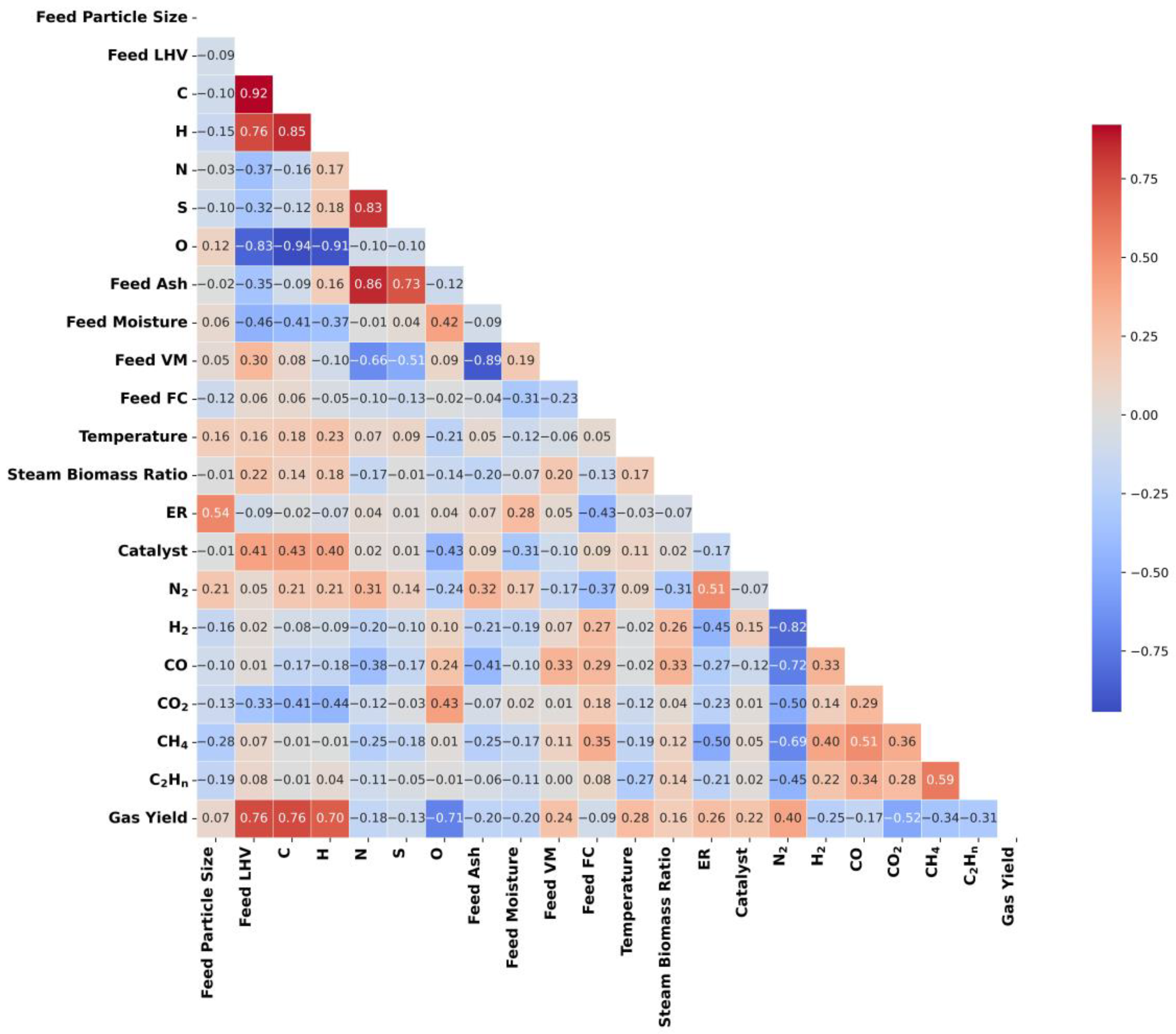
Exploratory data analysis is crucial for understanding relationships and patterns within a dataset. To this end, a correlation heat map was generated using Pearson’s correlation coefficient, which measures the linear dependence between pairs of continuous variables (Figure 3). This visualization helps identify variables that are highly correlated and may influence the performance of predictive models. Pearson’s coefficient, which ranges from −1 to +1, indicates the degree of association between two variables: values close to ±1 reflect a strong linear relationship, whereas values near 0 suggest a weak or non-existent relationship. This analysis provides valuable insight into which input variables significantly affect the response variables, aiding in the selection and optimization of predictive models.
The analysis in Figure 3 identifies the variables with the greatest influence on the syngas yield during the gasification process. The lower heating value (LHV) of the feedstock shows a strong positive correlation (0.76) with syngas yield, indicating that raw materials with higher energy content promote greater conversion to useful gas. Similarly, carbon (0.76) and hydrogen (0.70) contents are strongly associated with higher syngas yields, as these elements are the main precursors in the formation of combustible gases such as carbon monoxide (CO), hydrogen (H2), methane (CH4), and light hydrocarbons (C2Hn). Conversely, there is a strong negative correlation (−0.82) between H2 and N2, indicating that conditions favoring hydrogen production also reduce nitrogen content in the product gas. Therefore, minimizing N2 is key to maximizing H2 and improving the quality of the synthesis gas generated in gasification.
The oxygen content shows a strong negative correlation with both the LHV of the biomass (−0.83) and the syngas yield (−0.71), indicating that higher oxygen content in the raw material reduces its capacity to generate useful energy, thereby directly affecting syngas yield. Oxygen content also exhibits strong negative correlations with C (−0.94) and H (−0.91), meaning that as the proportion of oxygen increases, the proportions of carbon and hydrogen decrease significantly.
In addition, variable C shows a high correlation with the feed LHV (0.92) and with H (0.76), suggesting that carbon content is directly related to both the feed LHV and the hydrogen content of the material. In other words, higher carbon content in the feed corresponds to higher calorific value and hydrogen content. Similarly, N exhibits strong correlations with S (0.83) and with feed ash (0.86), indicating that increases in ash content are accompanied by increases in nitrogen content, and vice versa. Feed volatile matter and feed ash display an inverse correlation (−0.89), meaning that higher volatile matter content is associated with lower ash content. Finally, variables such as sulfur (S) and nitrogen (N) content show weak or neutral correlations with process efficiency, suggesting a limited impact on performance but potential environmental implications.
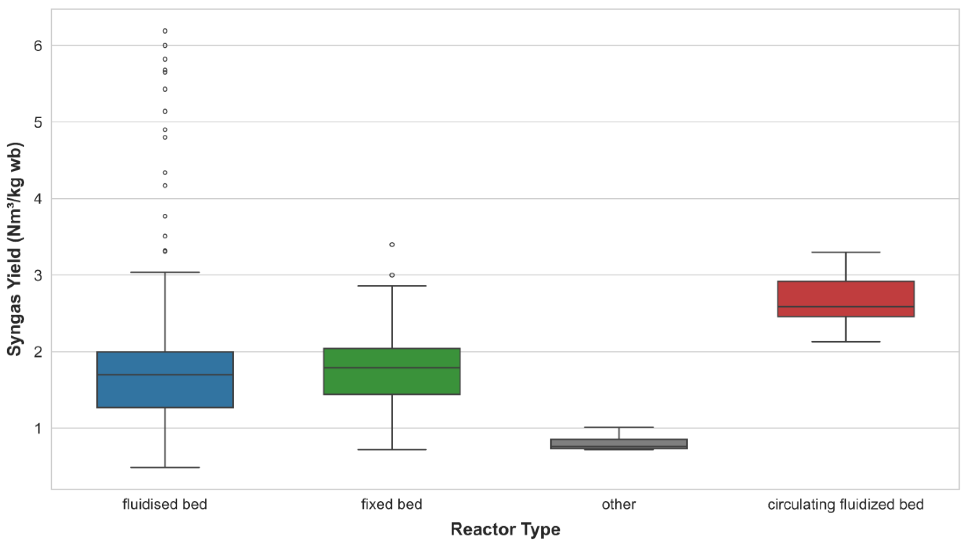
The analysis of syngas yield by reactor type showed that the circulating fluidized bed reactor delivers the best yield, with low data dispersion, indicating its suitability for efficient and controllable gasification processes (Figure 4). This superior performance can be attributed to better temperature distribution, more efficient mixing of reactants, and improved control over residence time, which together enhance process stability and promote uniform biomass conversion. In contrast, the fluidized bed reactor exhibited more variable performance and several extreme values, suggesting lower reliability due to the difficulty in predicting its behavior. This variability may be attributed to poor distribution of the gasifying agent or sensitivity to operating conditions, both of which hinder precise process control.

3.2. Machine Learning Results

The following variables were selected as input variables: gasifying agent, equivalence ratio (ER), Temperature, Carbon (C), Hydrogen (H), Nitrogen (N), Sulfur (S), Oxygen (O), feed Ash, feed Moisture, Volatile matter, Fixed carbon, Scale, Reactor type, steam/biomass, Catalyst used, Bed material, Operating mode, and feed LHV (see Table 1). The following were selected as output variables: the contents of N2, H2, CO, CO2, CH4, and C2Hn in the synthesis gas, as well as the syngas yield (see Table 2). Categorical variables (gasifying agent, system scale, reactor type, catalyst used, bed material, and operating condition) allow for capturing factors critical to gasification.
The ANN, Random Forest, and CatBoost models were used to predict the seven output variables, performing rigorous hyperparameter tuning via Bayesian optimization with Optuna, conducting 500 experiments per model. During this optimization process, key parameters were adjusted (see Table 3) to maximize predictive accuracy and minimize model error, ensuring adequate generalization across the entire test dataset. In addition, the RMSE of the test set was used as the loss function to be minimized, enabling the optimization to focus on improving the model’s overall performance while mitigating potential overfitting. The hyperparameter search bounds, shown in Table 3, were carefully selected to cover a wide range, allowing efficient exploration of possible configurations.
Table 4 presents the optimal values obtained after the optimization process, along with the average computation time recorded during Bayesian optimization for each evaluated model. It is important to note that the optimal values obtained were located in intermediate positions within the limits established for the hyperparameters (see Table 3), indicating that the defined search range was appropriate and sufficient to capture optimal configurations. This demonstrates that there is no need to expand the search space, as the optimal structures achieved do not correspond to overly complex models. This balance between simplicity and performance not only improves computational efficiency but also ensures robust and reliable prediction performance.
It is evident that some variables can be predicted more accurately than others. For example, the highest R2 among the seven output variables across the three models was 0.9860, achieved by the ANN model for predicting the N2 content of the synthesis gas. This same variable also had the lowest RMSE, at 0.0146. Conversely, the C2Hn content of the synthesis gas proved challenging for all models, as they achieved relatively low values across the different metrics. For this output variable, the ANN model recorded the lowest R2 (0.5949) and the highest RMSE (0.5038). All models showed excellent performance in predicting syngas yield, with R2 values above 0.9181; however, the ANN model achieved the best prediction, with an R2 of 0.9463 and the lowest RMSE of 0.0687 for this variable.
The results presented in Table 5 indicate that the CatBoost, Random Forest, and ANN models are effective in predicting the variables N2, H2, CO, CO2, CH4, C2Hn, and syngas yield. While all three models demonstrate excellent performance, the ANN stands out for its consistency and generalization ability, particularly in predicting N2. The accuracy achieved validates the feature selection and preprocessing methods applied, as well as the hyperparameter optimization performed for each model. These findings highlight the feasibility of using these ML approaches to model and predict complex parameters in biomass gasification.
Furthermore, Table 5 presents, for the ANN model, the mean ± standard deviation of the performance metrics (RMSE, MAE, R2, and R var _ weighted 2 ) obtained from the 5-fold cross-validation. Cross-validation is applied only to the ANN because it is identified as the best-performing model in the comparative analysis with Random Forest and CatBoost. The low standard deviations confirm the stability and consistency of the ANN predictions across the different training–validation partitions. The global value of R var _ weighted 2 (0.944 ± 0.032) indicates that, when all seven output variables are considered together and weighted by their variances, the ANN explains about 94% of the total variance, underscoring its overall predictive capability.
Several previous studies have applied simplified predictive approaches, such as thermodynamic equilibrium models, linear regressions, and semi-empirical correlations, to estimate syngas composition. For example, Huang and Ramaswamy [65] used an equilibrium model to approximate gas composition but could not represent secondary reactions accurately. Likewise, Várhegyi et al. [66] proposed empirical kinetic models with CO2 that performed well only within narrow operating ranges, while Silva et al. [67] developed a semi-empirical model combining stoichiometric balances with empirical corrections for methane and tars, whose validity remains limited to specific conditions. Although valuable in certain contexts, these approaches show lower accuracy and limited generalization when the operating domain is expanded. By contrast, the ML surrogates implemented here, trained on a large and heterogeneous multi-study database and validated through k-fold cross-validation, capture complex nonlinear relationships and achieve superior predictive performance (Table 5 and Table 6), thus providing a more robust and generalizable framework for biomass gasification modeling.
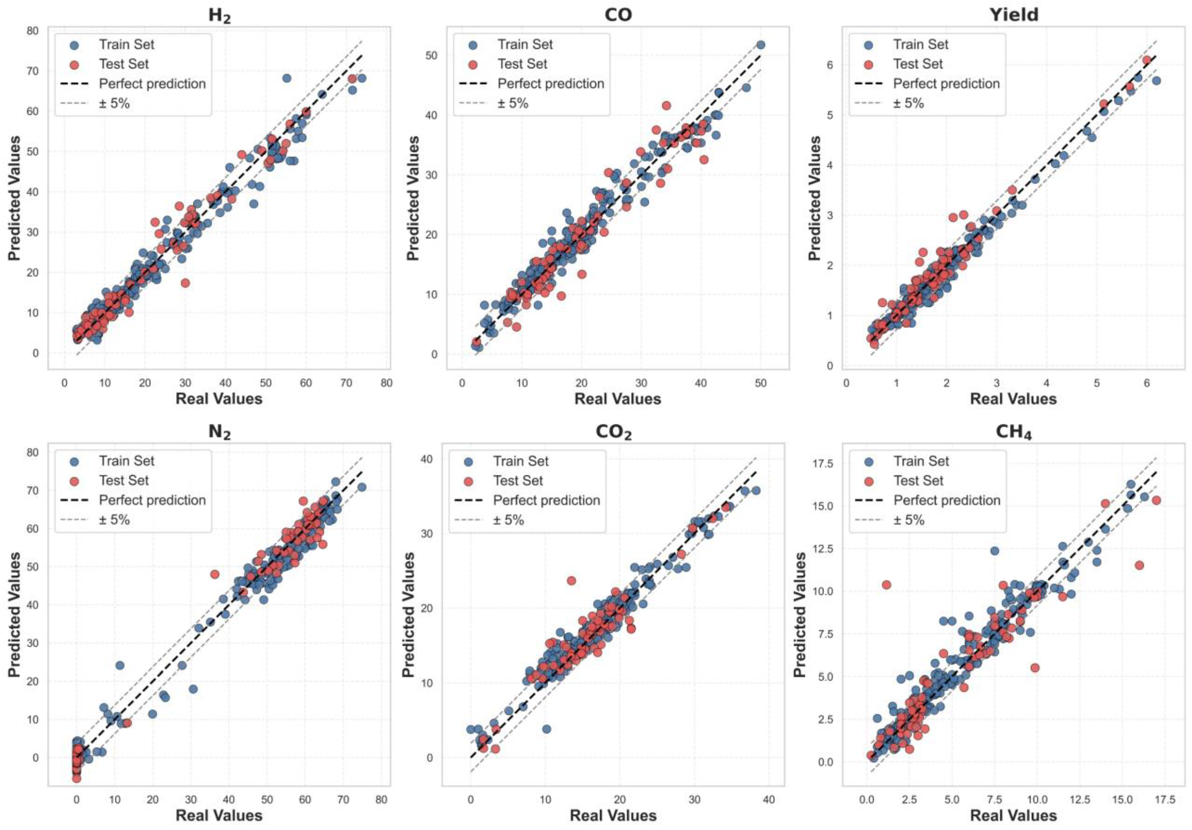
Figure 5 shows the prediction accuracy for N2, H2, CO, CO2, CH4, and syngas yield using the best-performing model (ANN). The results correspond to the training set and the validation set. Each graph includes a perfect prediction line (black), which serves as a reference for evaluating model accuracy; the closer the points lie to this line, the higher the prediction accuracy. The model predicts some variables more accurately than others; however, the model demonstrates generally good predictive performance (Table 6).
For the main components of syngas (H2, CO, CH4, and CO2), the model shows good prediction performance, supporting its practical utility in gasification process optimization. However, light hydrocarbons show lower R2 values (0.5949). Light hydrocarbons are usually not quantified with the same precision in all studies; unlike the main syngas gases, they are produced in lower concentrations and with greater measurement errors, resulting in a decrease in the quality of the data used to train the model. Furthermore, they are not the main target in the context of gasification process optimization, since they contribute insignificantly to the calorific value of the gas compared to more relevant compounds such as H2 and CO. Therefore, this limited performance does not compromise the overall validity of the model. However, based on the chemistry of gasification, the model does capture expected overall trends, such as the decrease in C2Hn with increasing temperature or equivalence ratio, confirming its qualitative consistency. This result should be understood as a limitation of the nature of the compound rather than a flaw or deficiency of the model.
Figure 6 presents an analysis of SHAP values to evaluate the contribution of each input variable in predicting the output variables with the highest accuracy in the models (N2, H2, CO, and syngas yield). This method provides a quantitative measure of the impact of both numerical and categorical input variables on the predictive model, offering detailed insights into the relative importance of each feature in the prediction process. The horizontal axis represents the SHAP value, i.e., the effect (positive or negative) of that variable on the predicted output, while the color intensity indicates whether the feature value is relatively high (pink) or low (blue).
Since the gasifying agent is a categorical variable, it was found to have the greatest impact on the four output variables. This impact varies significantly depending on the agent used, indicating a strong dependence of the system’s behavior on the gasification medium. In this study, five types of gasifying agents were considered: air, air + steam, oxygen, steam, and others (uncommon), each exerting different effects on the process. These results highlight the critical importance of selecting the appropriate gasifying agent to optimize the production and composition of syngas. In contrast, the mode of operation had the least influence on predicting the four output variables.
Another factor that had a significant impact on the output variables N2, H2, and syngas yield was the ER. In the specific case of H2 and syngas yield, the SHAP graph shows that low ER values have a positive impact on their prediction, as they favor a reducing environment in which hydrogen generation is maximized. Conversely, low ER values have a negative impact on the prediction of N2 in the output gas, since introducing less air also reduces the amount of inert nitrogen entering the system.
In addition, the LHV of the feedstock had a positive impact on gas yield. According to the SHAP analysis, high LHVs favor gas yield prediction because biomass with a high LHV contains larger amounts of combustible organic compounds, both volatile matter and fixed carbon, which are directly responsible for forming gases such as CO, H2, and CH4.
Fixed carbon in the feedstock had a significant positive impact on CO prediction. As shown in the corresponding SHAP graph, high fixed carbon values are associated with increased CO concentrations in syngas. This is because fixed carbon represents the non-volatile solid fraction that remains after pyrolysis and serves as the main reactant in gasification reactions. A higher fixed carbon content provides more active carbonaceous material for CO generation, thereby enhancing both solid conversion and the energy quality of the syngas.
The system scale was highly significant for the four output variables. For N2, a negative correlation was observed, likely because larger-scale systems generally do not use air as a gasifying agent, resulting in lower N2 concentrations. Conversely, these same conditions favor H2 and CO generation, as using gasifying agents other than air increases the production of these combustible gases. In contrast, the model indicated a negative effect of system scale on syngas yield.
Another characteristic that had a significant impact on the composition of the syngas was the steam/biomass ratio. Higher proportions of steam were associated with lower N2 concentrations, likely due to reduced use of air as a gasifying agent. Conversely, increasing this parameter led to higher H2 production. These contrasting effects make the steam/biomass ratio a critical variable for optimizing the quality and efficiency of the gasification process.
Although this study focuses on compounds that maximize syngas yield, it is also essential to assess two major greenhouse gases (CO2 and CH4) because of their key role in the overall environmental impact of biomass gasification. Including these species in the analysis not only supports the optimization of energy efficiency but also provides a more comprehensive environmental assessment.
Figure 7 shows, through a SHAP analysis, that CO2 generation is strongly dependent on variables such as the gasifying agent, feed LHV, and reactor type. Furthermore, high steam biomass ratio and low feed moisture levels favor its formation. Therefore, its yield can be controlled depending on the type of biomass used, as well as the process conditions. On the other hand, CH4 is also strongly related to the gasifying agent, this being the characteristic that has the greatest impact on its generation. Furthermore, it was observed that low values of ER, S, and temperature promote its production, which allows identifying strategies to moderate its emissions, such as the appropriate selection of the gasifying agent, the adjustment of the steam/biomass ratio to reduce CO2, and the control of ER and temperature to minimize CH4.

3.3. Multi-Objective Optimization Results

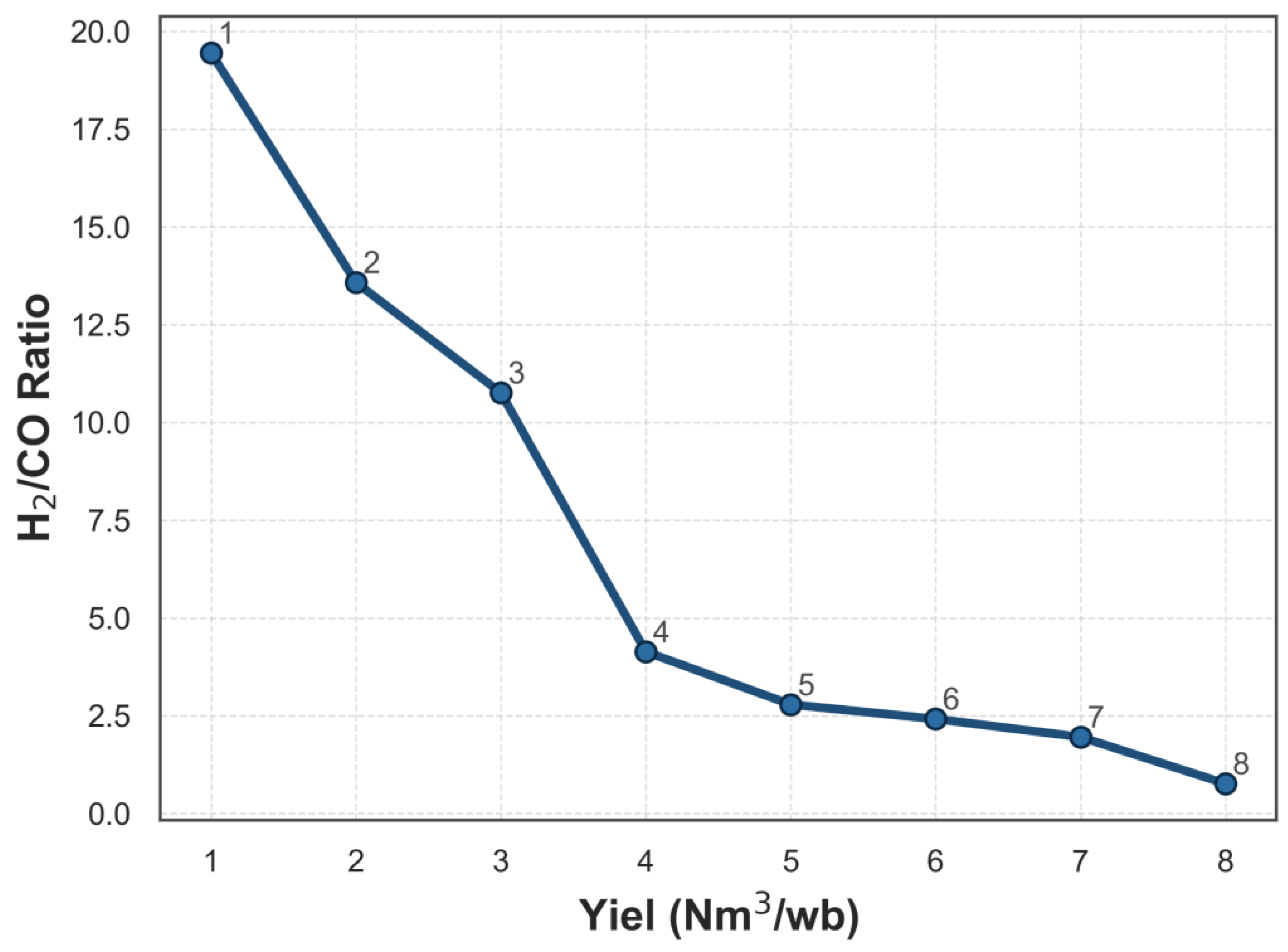
Figure 8 shows the resulting Pareto curve, which illustrates the inherent trade-off between maximizing the H2/CO ratio and maximizing syngas yield. Each point on the Pareto front represents an “optimal” solution in which improving one objective necessarily worsens the other; that is, no single configuration simultaneously optimizes both. The curve is generated using the ε-constraint method, in which one objective is directly optimized while the second is imposed as a constraint through a varying ε parameter to trace the trade-off front. The previously trained ANN, identified as the best-performing predictive model (see Table 6), is integrated into the optimization framework through the OMLT library. In particular, the ANN is reformulated in Pyomo using the ReluComplementarityFormulation, which converts the ReLU activations into algebraic constraints and initially yields a nonlinear programming (NLP) representation. This ReluComplementarityFormulation has already demonstrated excellent computational performance compared with other state-of-the-art ReLU reformulations, as reported by López Flores et al. [13]. Because the ANN includes categorical inputs encoded by one-hot encoding, these categorical features are represented as binary decision variables, ensuring that the categorical logic is preserved during the optimization. As a result, the overall formulation becomes a mixed-integer nonlinear program (MINLP), which is solved with the DICOPT solver using its default convergence tolerances.
For each Pareto-optimal point obtained with the ε-constraint strategy, the resulting MINLP contains approximately 916 constraints and 739 variables, of which 18 are binary and 721 are continuous. Each individual ε-constraint optimization was solved using DICOPT on an HP ZBook 17 G3 workstation (Intel Core i7-6700HQ CPU, 2.60 GHz; 32 GB RAM; AMD FirePro W6150M GPU with 4 GB). The average time required to obtain each point on the Pareto curve was approximately 1.6 s, with normal optimal termination.
There is a thermodynamic and design trade-off between increasing the H2/CO ratio and maximizing syngas yield [68]. Increasing steam (i.e., a higher steam/biomass ratio) promotes the water–gas shift reaction, raises the H2/CO ratio, and enriches the syngas with hydrogen. However, it also consumes CO, generates CO2, and requires more energy, ultimately reducing the volume of usable gas and carbon efficiency. Conversely, operating with less steam and limited oxidation favors CO formation and increases gas yield, although the resulting syngas is poorer in H2 [68,69]. Therefore, it is not possible to simultaneously optimize both objectives; a balance must be selected along the Pareto front, consistent with chemical equilibrium constraints and the elemental composition of the feedstock.
From a process design perspective, interpreting this trade-off is crucial for adapting synthesis gas to different industrial applications. The Pareto front, therefore, essentially offers a “menu” of optimal operating options based on the desired priorities (Figure 8), with different regions of the front being preferable depending on the intended end use of the syngas.
The high H2/CO ratio region (>10) of the Pareto front prioritizes syngas that is very rich in H2, at the expense of lower yield. This configuration is ideal for applications requiring nearly pure hydrogen, such as PEM fuel cells (which tolerate CO only in the ppm range) and ammonia synthesis (where CO poisons the iron catalyst) [70]. The intermediate region, with H2/CO ratios close to 2, offers an optimal compromise between a high hydrogen fraction and good syngas yield. This makes it particularly suitable for methanol (CH3OH) synthesis (stoichiometric ratio of 2:1 H2 to CO) [71] and Fischer–Tropsch (FT) synthesis. In FT processes, cobalt catalysts perform optimally at ratios around 1.8–2.2, while iron catalysts tolerate slightly lower ratios due to their intrinsic shift activity [72]. Operationally, conditions such as moderate steam input and beds or catalysts that balance H2 and CO facilitate reaching this region. Therefore, these results confirm that targeting H2/CO ratios close to 2 on the Pareto front maximizes conversion efficiency and minimizes rework in downstream processing stages. The low H2/CO ratio region (less than 1) corresponds to CO-rich syngas with high overall yield, making it ideal when CO is the primary reactant, and excess hydrogen does not add value [71]. Typical examples include dimethyl ether (DME) synthesis, which operates efficiently at H2/CO ratios close to 1, consistent with syngas produced by O2-fed gasifiers without steam (entrained-flow), typically in the range of 0.7–1.0. Thermodynamically, this regime results from low steam input and sufficient partial oxidation to favor CO formation, thereby increasing gas volume per kilogram of biomass [71]. The opportunity cost at these ratios is a lower hydrogen content, which is acceptable when the subsequent stage of the process consumes CO as the main reactant (e.g., routes to heavy hydrocarbons, higher alcohols, or direct mineral reduction).
The Pareto curve serves as a design guide, enabling the selection of the operating point based on the intended application of the syngas: a high H2/CO ratio for hydrogen production (e.g., PEM fuel cells or ammonia synthesis), accepting lower yield; an intermediate H2/CO ratio (~2) for methanol or FT synthesis, balancing purity and flow rate; and a low H2/CO ratio when CO is the primary reactant and yield is prioritized. This approach, supported by multi-objective analysis, requires integrating thermodynamic considerations (equilibria and elemental utilization) with downstream process requirements. In practice, the Pareto front quantifies the performance trade-off between purity and yield (or vice versa), enabling a customized design of biomass systems, syngas composition, and final product characteristics.
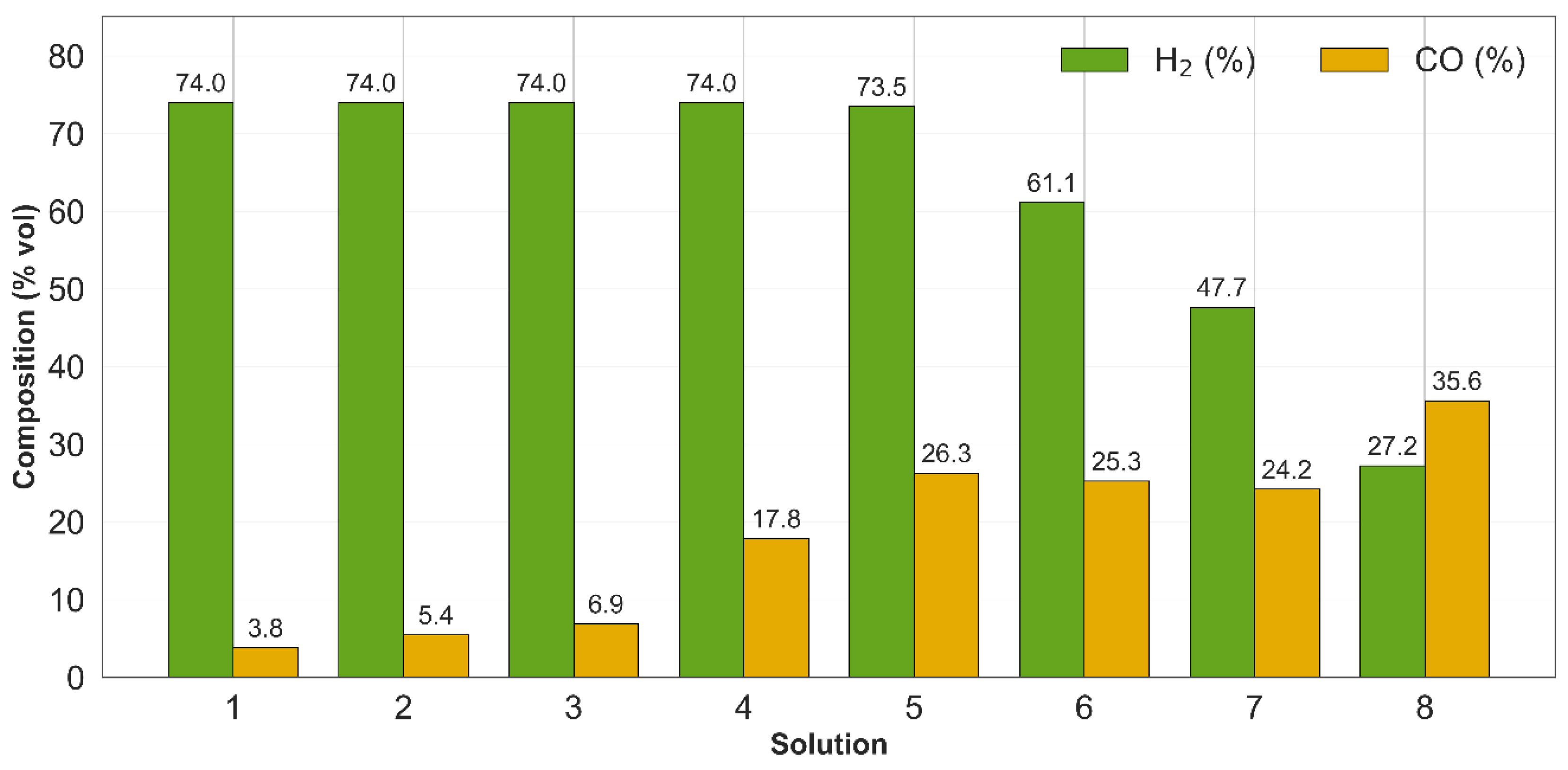
Furthermore, Figure 9 shows the output composition (H2 and CO) for the eight optimal solutions. In the low-yield regime (solutions 1–4), the syngas is dominated by H2, with concentrations close to 74% vol., while CO exhibits only moderate increases (3.8–17.8% vol.). As the operation shifts toward higher yields (solutions 5–8), a sustained decrease in the H2 fraction (from 73.5% to 27.2% vol.) and an increase in CO (from 26.3% to 35.6% vol.) are observed. In solution 8, CO exceeds H2, indicating a change in the compositional regime. This behavior is consistent with the trade-off identified between maximizing the H2/CO ratio and the total syngas yield: conditions that increase yield tend to favor CO formation and retention, while reducing the fraction of available hydrogen.
Table 7 summarizes the optimal conditions identified for solutions 1, 2, 6, 7, and 8 on the Pareto front. As shown, moving toward higher-performance solutions is associated with an increase in the ER and a decrease in the steam/biomass ratio, shifting the stoichiometry toward CO-rich syngas and reducing the H2/CO ratio. Temperature does not exhibit a monotonic trend and acts instead as a kinetic–thermodynamic modulator. Notably, the SHAP analysis results corroborate these behaviors. Reactor type also covaries with performance: the fluidized bed is associated with higher yields, while the fixed bed appears in solutions with a high H2/CO ratio. Bed materials and catalysts promote cracking/reforming reactions and tar control, reinforcing the role of the gasifier–ER pair. Finally, feedstock composition influences the C–H–O balance: higher carbon and lower oxygen contents tend to increase CO production, while moisture and volatile matter contribute to H2 generation in the presence of steam and catalytic activity for water–gas shift and reforming reactions. Overall, the results align with the behavior observed on the Pareto front: higher yields are generally associated with lower H2/CO ratios, and vice versa.
It is important to note that each decision variable is restricted to the valid range reported in Table 1, ensuring that the optimization remains within physically realistic conditions and inside the training domain of the surrogate model. These bounds act as explicit constraints in the optimization model. No extra strengthening techniques, such as convex-hull reformulations or trust-region restrictions, are implemented because the complementarity formulation already converges efficiently, and the decision variables are explicitly bounded. The choice of ReluComplementarityFormulation over convex-hull alternatives balances model fidelity and computational complexity. Post-optimization interpretability analyses (e.g., SHAP or partial-dependence plots) are not performed since the objective of this study is the identification of optimal operating conditions using the surrogate model rather than an in-depth analysis of model explainability. All reported optima are directly verified to satisfy the original constraints and to deliver the expected improvements in the target objectives.

4. Conclusions

This study is the first to combine advanced ML surrogates with a multi-objective optimization framework for biomass gasification. It demonstrates that integrating ML models with multi-objective optimization is an effective approach for simultaneously predicting and maximizing the production and quality of synthesis gas. Using a large and heterogeneous database comprising 343 experimental records from 33 previous studies, covering multiple types of biomasses, gasifying agents, reactor configurations, and bed materials, it was possible to train and validate ANN, Random Forest, and CatBoost models with high levels of accuracy, with the ANN standing out for its ability to generalize and consistently predict multiple key variables.
The interpretability analysis using the SHAP method enabled the identification and ranking of the variables with the greatest impact on predictions. Among these, the gasifying agent, ER, LHV, fixed carbon content, and steam/biomass ratio exhibited a decisive influence on the composition and yield of the produced gas. In particular, the type of gasifying agent proved to be the most influential factor, indicating that proper selection of this parameter is critical for maximizing H2 content and controlling the N2 fraction. Furthermore, low ER values were found to favor H2 production and reduce nitrogen content, while higher ER values promoted CO formation, directly affecting the H2/CO ratio. Similarly, the LHV and fixed carbon content were positively associated with yield and CO fraction, underscoring the importance of the intrinsic properties of the feedstock in the overall performance of the process.
The integration of the ANN model into a multi-objective optimization framework enabled the plotting of the Pareto frontier, which describes the trade-off between total syngas yield and the H2/CO ratio. The results show that it is not possible to simultaneously maximize both variables—high steam/biomass ratios and the use of steam or oxygen favor H2 content—but reduce the total yield, whereas low steam/biomass ratios and partial oxidation increase yield and CO content, thereby decreasing H2. This trade-off allows for the definition of operating zones according to the intended end use: H2/CO ratios greater than 10 for pure hydrogen, close to 2 for methanol and Fischer–Tropsch synthesis, and less than 1 for processes where CO predominates, such as DME production or direct reduction. Furthermore, the analysis of optimal solutions revealed that higher ER values combined with lower steam/biomass ratios shift the operation toward higher yields but lower H2/CO ratios.
The predictive models developed in this work are data-driven and were trained on a compiled literature dataset. Therefore, their predictions are reliable only within the range of operating conditions and feedstock properties represented in the training data. Extrapolating the models to conditions that fall outside these ranges should be interpreted with caution, as the associated prediction uncertainty may increase substantially.
In methodological terms, this study underscores the value of using large and diverse experimental databases, as well as the importance of incorporating categorical variables into modeling to capture operational and design effects that cannot be explained solely by numerical data. Hyperparameter optimization using Bayesian approaches (Optuna) proved to be an effective strategy for balancing accuracy and generalization capacity, avoiding overparameterization and reducing computational costs.
Overall, the proposed methodology constitutes an effective and adaptable tool for modeling and optimizing biomass gasification, facilitating decision-making and improving both technical and energy performance while promoting waste recovery and clean energy production.

Author Contributions

Conceptualization, G.B.-B., F.J.L.-F. and J.M.P.-O.; methodology, G.B.-B. and F.J.L.-F.; formal analysis, G.B.-B., F.J.L.-F., E.R.-C. and J.M.P.-O.; investigation, G.B.-B., F.J.L.-F., E.R.-C. and J.M.P.-O.; resources, J.M.P.-O.; data curation, G.B.-B. and F.J.L.-F.; writing—original draft preparation, G.B.-B., F.J.L.-F. and J.M.P.-O.; writing—review and editing, G.B.-B., F.J.L.-F., E.R.-C. and J.M.P.-O.; visualization, G.B.-B. and F.J.L.-F.; supervision, F.J.L.-F., E.R.-C. and J.M.P.-O.; project administration, F.J.L.-F. and J.M.P.-O.; funding acquisition, J.M.P.-O. All authors have read and agreed to the published version of the manuscript.

Funding

This research received no external funding.

Data Availability Statement

The data used in this study are available upon request.

Acknowledgments

The authors appreciate the support provided by the Secretaría de Ciencia, Humanidades, Tecnología e Innovación (SECIHTI), and the Coordinación de la Investigación Científica of the Universidad Michoacana de San Nicolás de Hidalgo (CIC-UMSNH).

Conflicts of Interest

The authors declare no conflicts of interest.

Abbreviations

The following abbreviations are used in this manuscript:
ANNArtificial neural network
dafDry and ash-free
dbDry basis
EREquivalence ratio
FCFixed carbon
FTFischer–Tropsch
LHVLower heating value
MAEMean absolute error
MAPEMean absolute percentage error
MILPMixed-integer linear programming
MLMachine learning
MLPMulti-layer perceptron
MSWMunicipal solid waste
NLPNonlinear programming
OFObjective function
OMLTOptimization and machine learning toolbox
R2Correlation coefficient
ReLURectified linear unit
RMSERoot mean square error
SHAPShapley additive explanations
TanhHyperbolic tangent
TPETree-structured Parzen Estimator
VMVolatile matter
wbWet basis
wtWeight
εMinimum acceptable syngas yield

References

  1. Fernando, S.; Adhikari, S.; Chandrapal, C.; Murali, N. Biorefineries:  Current Status, Challenges, and Future Direction. Energy Fuels 2006, 20, 1727–1737. [Google Scholar] [CrossRef]
  2. UNEP. Beyond an Age of Waste: Turning Rubbish into a Resource. In Global Waste Management Outlook; UNEP: Nairobi, Kenya, 2024; ISBN 978-92-807-4129-2. [Google Scholar]
  3. World Must Move beyond Waste Era and Turn Rubbish into Resource: UN Report. Available online: https://www.unep.org/news-and-stories/press-release/world-must-move-beyond-waste-era-and-turn-rubbish-resource-un-report (accessed on 12 August 2025).
  4. Gao, Y.; Wang, M.; Raheem, A.; Wang, F.; Wei, J.; Xu, D.; Song, X.; Bao, W.; Huang, A.; Zhang, S.; et al. Syngas Production from Biomass Gasification: Influences of Feedstock Properties, Reactor Type, and Reaction Parameters. ACS Omega 2023, 8, 31620–31631. [Google Scholar] [CrossRef]
  5. Ascher, S.; Sloan, W.; Watson, I.; You, S. A Comprehensive Artificial Neural Network Model for Gasification Process Prediction. Appl. Energy 2022, 320, 119289. [Google Scholar] [CrossRef]
  6. López-Flores, F.J.; Ochoa-Barragán, R.; Raya-Tapia, A.Y.; Ramírez-Márquez, C.; Ponce-Ortega, J.M. (Eds.) Chapter 17–Challenges and Future Scope. In Machine Learning Tools for Chemical Engineering; Elsevier: Amsterdam, Netherlands, 2025; pp. 591–598. ISBN 978-0-443-29058-9. [Google Scholar]
  7. Daoutidis, P.; Lee, J.H.; Rangarajan, S.; Chiang, L.; Gopaluni, B.; Schweidtmann, A.M.; Harjunkoski, I.; Mercangöz, M.; Mesbah, A.; Boukouvala, F.; et al. Machine Learning in Process Systems Engineering: Challenges and Opportunities. Comput. Chem. Eng. 2024, 181, 108523. [Google Scholar] [CrossRef]
  8. Baruah, D.; Baruah, D.C.; Hazarika, M.K. Artificial Neural Network Based Modeling of Biomass Gasification in Fixed Bed Downdraft Gasifiers. Biomass Bioenergy 2017, 98, 264–271. [Google Scholar] [CrossRef]
  9. Xiao, G.; Ni, M.; Chi, Y.; Jin, B.; Xiao, R.; Zhong, Z.; Huang, Y. Gasification Characteristics of MSW and an ANN Prediction Model. Waste Manag. 2009, 29, 240–244. [Google Scholar] [CrossRef] [PubMed]
  10. Serrano, D.; Golpour, I.; Sánchez-Delgado, S. Predicting the Effect of Bed Materials in Bubbling Fluidized Bed Gasification Using Artificial Neural Networks (ANNs) Modeling Approach. Fuel 2020, 266, 117021. [Google Scholar] [CrossRef]
  11. Elmaz, F.; Yücel, Ö.; Mutlu, A.Y. Predictive Modeling of Biomass Gasification with Machine Learning-Based Regression Methods. Energy 2020, 191, 116541. [Google Scholar] [CrossRef]
  12. Kardani, N.; Zhou, A.; Nazem, M.; Lin, X. Modelling of Municipal Solid Waste Gasification Using an Optimised Ensemble Soft Computing Model. Fuel 2021, 289, 119903. [Google Scholar] [CrossRef]
  13. López-Flores, F.J.; Ramírez-Márquez, C.; Ponce-Ortega, J.M. Process Systems Engineering Tools for Optimization of Trained Machine Learning Models: Comparative and Perspective. Ind. Eng. Chem. Res. 2024, 63, 13966–13979. [Google Scholar] [CrossRef]
  14. Ceccon, F.; Jalving, J.; Haddad, J.; Thebelt, A.; Tsay, C.; Laird, C.D.; Misener, R. OMLT: Optimization & Machine Learning Toolkit. arXiv 2022, arXiv:2202.02414. [Google Scholar] [CrossRef]
  15. Turner, M.; Chmiela, A.; Koch, T.; Winkler, M. PySCIPOpt-ML: Embedding Trained Machine Learning Models into Mixed-Integer Programs. arXiv 2024, arXiv:2312.08074. [Google Scholar]
  16. Dowson, O.; Parker, R.B.; Bent, R. MathOptAI.Jl: Embed Trained Machine Learning Predictors into JuMP Models. arXiv 2025, arXiv:2507.03159. [Google Scholar]
  17. López-Flores, F.J.; Lira-Barragán, L.F.; Rubio-Castro, E.; El-Halwagi, M.M.; Ponce-Ortega, J.M. Hybrid Machine Learning-Mathematical Programming Approach for Optimizing Gas Production and Water Management in Shale Gas Fields. ACS Sustain. Chem. Eng. 2023, 11, 6043–6056. [Google Scholar] [CrossRef]
  18. Hou, S.; Duque, E.M.S.; Palensky, P.; Vergara, P.P. A Constraint Enforcement Deep Reinforcement Learning Framework for Optimal Energy Storage Systems Dispatch. arXiv 2023, arXiv:2307.14304. [Google Scholar] [CrossRef]
  19. Bugosen, S.I.; Laird, C.D.; Parker, R.B. Process Flowsheet Optimization with Surrogate and Implicit Formulations of a Gibbs Reactor. arXiv 2024, arXiv:2310.09307. [Google Scholar] [CrossRef]
  20. Jalving, J.; Ghouse, J.; Cortes, N.; Gao, X.; Knueven, B.; Agi, D.; Martin, S.; Chen, X.; Guittet, D.; Tumbalam-Gooty, R.; et al. Beyond Price Taker: Conceptual Design and Optimization of Integrated Energy Systems Using Machine Learning Market Surrogates. Appl. Energy 2023, 351, 121767. [Google Scholar] [CrossRef]
  21. López-Flores, F.J.; Ramírez-Márquez, C.; Rubio-Castro, E.; Ponce-Ortega, J.M. Solar Photovoltaic Panel Production in Mexico: A Novel Machine Learning Approach. Environ. Res. 2024, 246, 118047. [Google Scholar] [CrossRef]
  22. Padilla-Esquivel, C.A.; López-Flores, F.J.; Hernández-Pérez, L.G.; Rubio-Castro, E.; Ponce-Ortega, J.M. Optimizing Green Urea Production: Integration of Process Simulation, Artificial Intelligence, and Sustainable Technologies. J. Clean. Prod. 2025, 501, 145371. [Google Scholar] [CrossRef]
  23. Mansaray, K.G.; Ghaly, A.E.; Al-Taweel, A.M.; Hamdullahpur, F.; Ugursal, V.I. Air Gasification of Rice Husk in a Dual Distributor Type Fluidized Bed Gasifier. Biomass Bioenergy 1999, 17, 315–332. [Google Scholar] [CrossRef]
  24. De Andrés, J.M.; Narros, A.; Rodríguez, M.E. Air-Steam Gasification of Sewage Sludge in a Bubbling Bed Reactor: Effect of Alumina as a Primary Catalyst. Fuel Process. Technol. 2011, 92, 433–440. [Google Scholar] [CrossRef]
  25. Lv, P.M.; Xiong, Z.H.; Chang, J.; Wu, C.Z.; Chen, Y.; Zhu, J.X. An Experimental Study on Biomass Air–Steam Gasification in a Fluidized Bed. Bioresour. Technol. 2004, 95, 95–101. [Google Scholar] [CrossRef]
  26. Fremaux, S.; Beheshti, S.-M.; Ghassemi, H.; Shahsavan-Markadeh, R. An Experimental Study on Hydrogen-Rich Gas Production via Steam Gasification of Biomass in a Research-Scale Fluidized Bed. Energy Convers. Manag. 2015, 91, 427–432. [Google Scholar] [CrossRef]
  27. Sarker, S.; Nielsen, H.K. Assessing the Gasification Potential of Five Woodchips Species by Employing a Lab-Scale Fixed-Bed Downdraft Reactor. Energy Convers. Manag. 2015, 103, 801–813. [Google Scholar] [CrossRef]
  28. Lv, P.; Chang, J.; Xiong, Z.; Huang, H.; Wu, C.; Chen, Y.; Zhu, J. Biomass Air−Steam Gasification in a Fluidized Bed to Produce Hydrogen-Rich Gas. Energy Fuels 2003, 17, 677–682. [Google Scholar] [CrossRef]
  29. Miccio, F.; Piriou, B.; Ruoppolo, G.; Chirone, R. Biomass Gasification in a Catalytic Fluidized Reactor with Beds of Different Materials. Chem. Eng. J. 2009, 154, 369–374. [Google Scholar] [CrossRef]
  30. Li, X.T.; Grace, J.R.; Lim, C.J.; Watkinson, A.P.; Chen, H.P.; Kim, J.R. Biomass Gasification in a Circulating Fluidized Bed. Biomass Bioenergy 2004, 26, 171–193. [Google Scholar] [CrossRef]
  31. Narváez, I.; Orío, A.; Aznar, M.P.; Corella, J. Biomass Gasification with Air in an Atmospheric Bubbling Fluidized Bed. Effect of Six Operational Variables on the Quality of the Produced Raw Gas. Ind. Eng. Chem. Res. 1996, 35, 2110–2120. [Google Scholar] [CrossRef]
  32. Baratieri, M.; Pieratti, E.; Nordgreen, T.; Grigiante, M. Biomass Gasification with Dolomite as Catalyst in a Small Fluidized Bed Experimental and Modelling Analysis. Waste Biomass Valorization 2010, 1, 283–291. [Google Scholar] [CrossRef]
  33. Sarker, S.; Bimbela, F.; Sánchez, J.L.; Nielsen, H.K. Characterization and Pilot Scale Fluidized Bed Gasification of Herbaceous Biomass: A Case Study on Alfalfa Pellets. Energy Convers. Manag. 2015, 91, 451–458. [Google Scholar] [CrossRef]
  34. Biagini, E.; Barontini, F.; Tognotti, L. Development of a Bi-Equilibrium Model for Biomass Gasification in a Downdraft Bed Reactor. Bioresour. Technol. 2016, 201, 156–165. [Google Scholar] [CrossRef]
  35. Dutta, P.P.; Pandey, V.; Das, A.R.; Sen, S.; Baruah, D.C. Down Draft Gasification Modelling and Experimentation of Some Indigenous Biomass for Thermal Applications. Energy Procedia 2014, 54, 21–34. [Google Scholar] [CrossRef]
  36. Loha, C.; Chattopadhyay, H.; Chatterjee, P.K. Energy Generation from Fluidized Bed Gasification of Rice Husk. J. Renew. Sustain. Energy 2013, 5, 043111. [Google Scholar] [CrossRef]
  37. Zhang, Z.; Pang, S. Experimental Investigation of Biomass Devolatilization in Steam Gasification in a Dual Fluidised Bed Gasifier. Fuel 2017, 188, 628–635. [Google Scholar] [CrossRef]
  38. Song, T.; Wu, J.; Shen, L.; Xiao, J. Experimental Investigation on Hydrogen Production from Biomass Gasification in Interconnected Fluidized Beds. Biomass Bioenergy 2012, 36, 258–267. [Google Scholar] [CrossRef]
  39. Karatas, H.; Akgun, F. Experimental Results of Gasification of Walnut Shell and Pistachio Shell in a Bubbling Fluidized Bed Gasifier under Air and Steam Atmospheres. Fuel 2018, 214, 285–292. [Google Scholar] [CrossRef]
  40. Liu, H.; Hu, J.; Wang, H.; Wang, C.; Li, J. Experimental Studies of Biomass Gasification with Air. J. Nat. Gas Chem. 2012, 21, 374–380. [Google Scholar] [CrossRef]
  41. Gai, C.; Dong, Y. Experimental Study on Non-Woody Biomass Gasification in a Downdraft Gasifier. Int. J. Hydrogen Energy 2012, 37, 4935–4944. [Google Scholar] [CrossRef]
  42. Arena, U.; Zaccariello, L.; Mastellone, M.L. Fluidized Bed Gasification of Waste-Derived Fuels. Waste Manag. 2010, 30, 1212–1219. [Google Scholar] [CrossRef]
  43. Arena, U.; Di Gregorio, F. Gasification of a Solid Recovered Fuel in a Pilot Scale Fluidized Bed Reactor. Fuel 2014, 117, 528–536. [Google Scholar] [CrossRef]
  44. Kaewluan, S.; Pipatmanomai, S. Gasification of High Moisture Rubber Woodchip with Rubber Waste in a Bubbling Fluidized Bed. Fuel Process. Technol. 2011, 92, 671–677. [Google Scholar] [CrossRef]
  45. Lahijani, P.; Zainal, Z.A. Gasification of Palm Empty Fruit Bunch in a Bubbling Fluidized Bed: A Performance and Agglomeration Study. Bioresour. Technol. 2011, 102, 2068–2076. [Google Scholar] [CrossRef]
  46. Ruoppolo, G.; Ammendola, P.; Chirone, R.; Miccio, F. H2-Rich Syngas Production by Fluidized Bed Gasification of Biomass and Plastic Fuel. Waste Manag. 2012, 32, 724–732. [Google Scholar] [CrossRef] [PubMed]
  47. Khan, Z.; Yusup, S.; Ahmad, M.M.; Chin, B.L.F. Hydrogen Production from Palm Kernel Shell via Integrated Catalytic Adsorption (ICA) Steam Gasification. Energy Convers. Manag. 2014, 87, 1224–1230. [Google Scholar] [CrossRef]
  48. Wang, J.; Cheng, G.; You, Y.; Xiao, B.; Liu, S.; He, P.; Guo, D.; Guo, X.; Zhang, G. Hydrogen-Rich Gas Production by Steam Gasification of Municipal Solid Waste (MSW) Using NiO Supported on Modified Dolomite. Int. J. Hydrogen Energy 2012, 37, 6503–6510. [Google Scholar] [CrossRef]
  49. Iovane, P.; Donatelli, A.; Molino, A. Influence of Feeding Ratio on Steam Gasification of Palm Shells in a Rotary Kiln Pilot Plant. Experimental and Numerical Investigations. Biomass Bioenergy 2013, 56, 423–431. [Google Scholar] [CrossRef]
  50. Erkiaga, A.; Lopez, G.; Amutio, M.; Bilbao, J.; Olazar, M. Influence of Operating Conditions on the Steam Gasification of Biomass in a Conical Spouted Bed Reactor. Chem. Eng. J. 2014, 237, 259–267. [Google Scholar] [CrossRef]
  51. Yin, R.; Liu, R.; Wu, J.; Wu, X.; Sun, C.; Wu, C. Influence of Particle Size on Performance of a Pilot-Scale Fixed-Bed Gasification System. Bioresour. Technol. 2012, 119, 15–21. [Google Scholar] [CrossRef]
  52. Huynh, C.V.; Kong, S.-C. Performance Characteristics of a Pilot-Scale Biomass Gasifier Using Oxygen-Enriched Air and Steam. Fuel 2013, 103, 987–996. [Google Scholar] [CrossRef]
  53. Carpenter, D.L.; Bain, R.L.; Davis, R.E.; Dutta, A.; Feik, C.J.; Gaston, K.R.; Jablonski, W.; Phillips, S.D.; Nimlos, M.R. Pilot-Scale Gasification of Corn Stover, Switchgrass, Wheat Straw, and Wood: 1. Parametric Study and Comparison with Literature. Ind. Eng. Chem. Res. 2010, 49, 1859–1871. [Google Scholar] [CrossRef]
  54. Herguido, J.; Corella, J.; Gonzalez-Saiz, J. Steam Gasification of Lignocellulosic Residues in a Fluidized Bed at a Small Pilot Scale. Effect of the Type of Feedstock. Ind. Eng. Chem. Res. 1992, 31, 1274–1282. [Google Scholar] [CrossRef]
  55. Luo, S.; Zhou, Y.; Yi, C. Syngas Production by Catalytic Steam Gasification of Municipal Solid Waste in Fixed-Bed Reactor. Energy 2012, 44, 391–395. [Google Scholar] [CrossRef]
  56. López-Flores, F.J.; Ochoa-Barragán, R.; Raya-Tapia, A.Y.; Ramírez-Márquez, C.; Ponce-Ortega, J.M. (Eds.) Chapter 9—Deep Learning. In Machine Learning Tools for Chemical Engineering; Elsevier: Amsterdam, Netherlands, 2025; pp. 241–291. ISBN 978-0-443-29058-9. [Google Scholar]
  57. Taud, H.; Mas, J.F. Multilayer Perceptron (MLP). In Geomatic Approaches for Modeling Land Change Scenarios; Camacho Olmedo, M.T., Paegelow, M., Mas, J.-F., Escobar, F., Eds.; Springer International Publishing: Cham, Switzerland, 2018; pp. 451–455. ISBN 978-3-319-60801-3. [Google Scholar]
  58. Cutler, A.; Cutler, D.R.; Stevens, J.R. Random Forests. In Ensemble Machine Learning: Methods and Applications; Zhang, C., Ma, Y., Eds.; Springer: New York, NY, USA, 2012; pp. 157–175. ISBN 978-1-4419-9326-7. [Google Scholar]
  59. Genuer, R.; Poggi, J.-M. (Eds.) Random Forests. In Random Forests with R; Springer International Publishing: Cham, Switzerland, 2020; pp. 33–55. ISBN 978-3-030-56485-8. [Google Scholar]
  60. Prokhorenkova, L.; Gusev, G.; Vorobev, A.; Dorogush, A.V.; Gulin, A. CatBoost: Unbiased Boosting with Categorical Features. arXiv 2019, arXiv:1706.09516. [Google Scholar] [CrossRef]
  61. Bentéjac, C.; Csörgő, A.; Martínez-Muñoz, G. A Comparative Analysis of Gradient Boosting Algorithms. Artif. Intell. Rev. 2021, 54, 1937–1967. [Google Scholar] [CrossRef]
  62. Zhou, Y.; Cahya, S.; Combs, S.A.; Nicolaou, C.A.; Wang, J.; Desai, P.V.; Shen, J. Exploring Tunable Hyperparameters for Deep Neural Networks with Industrial ADME Data Sets. J. Chem. Inf. Model. 2019, 59, 1005–1016. [Google Scholar] [CrossRef]
  63. Agrawal, T. (Ed.) Optuna and AutoML. In Hyperparameter Optimization in Machine Learning: Make Your Machine Learning and Deep Learning Models More Efficient; Apress: Berkeley, CA, USA, 2021; pp. 109–129. ISBN 978-1-4842-6579-6. [Google Scholar]
  64. Gridin, I. (Ed.) Hyperparameter Optimization. In Automated Deep Learning Using Neural Network Intelligence: Develop and Design PyTorch and TensorFlow Models Using Python; Apress: Berkeley, CA, USA, 2022; pp. 31–110. ISBN 978-1-4842-8149-9. [Google Scholar]
  65. Zol, S.; Chandodkar, H.; Ahmed, M.; Haider, M.B.; Kumar, K.D.P.L.; Naidu, B.N.; Kumar, R.; Viswanadham, N. Multi-Objective Optimization of Syngas Production from Bio-Glycerol: A Bi-Reforming Approach Using NSGA-II. J. Environ. Chem. Eng. 2025, 13, 116186. [Google Scholar] [CrossRef]
  66. Huang, H.; Ramaswamy, S. Modeling Biomass Gasification Using Thermodynamic Equilibrium Approach. Appl. Biochem. Biotechnol. 2009, 154, 14–25. [Google Scholar] [CrossRef] [PubMed]
  67. Várhegyi, G.; Wang, L.; Skreiberg, Ø. Empirical Kinetic Models for the CO2 Gasification of Biomass Chars. Part 1. Gasification of Wood Chars and Forest Residue Chars. ACS Omega 2021, 6, 27552–27560. [Google Scholar] [CrossRef] [PubMed]
  68. Silva, I.P.; Lima, R.M.; Santana, H.E.; Silva, G.F.; Ruzene, D.S.; Silva, D.P. Development of a Semi-Empirical Model for Woody Biomass Gasification Based on Stoichiometric Thermodynamic Equilibrium Model. Energy 2022, 241, 122894. [Google Scholar] [CrossRef]
  69. Aentung, T.; Patcharavorachot, Y.; Wu, W. Co-Gasification of Plastic Waste Blended with Biomass: Process Modeling and Multi-Objective Optimization. Processes 2024, 12, 1906. [Google Scholar] [CrossRef]
  70. Molochas, C.; Tsiakaras, P. Carbon Monoxide Tolerant Pt-Based Electrocatalysts for H2-PEMFC Applications: Current Progress and Challenges. Catalysts 2021, 11, 1127. [Google Scholar] [CrossRef]
  71. Rauch, R.; Hrbek, J.; Hofbauer, H. Biomass Gasification for Synthesis Gas Production and Applications of the Syngas. In Advances in Bioenergy; John Wiley & Sons, Ltd: Hoboken, NJ, USA, 2016; pp. 73–91. ISBN 978-1-118-95784-4. [Google Scholar]
  72. Lögdberg, S. Development of Fischer-Tropsch Catalysts for Gasified Biomass; School of Chemical Science and Engineering, Royal Institute of Technology: Stockholm, Sweden, 2007; ISBN 978-91-7178-698-2. [Google Scholar]
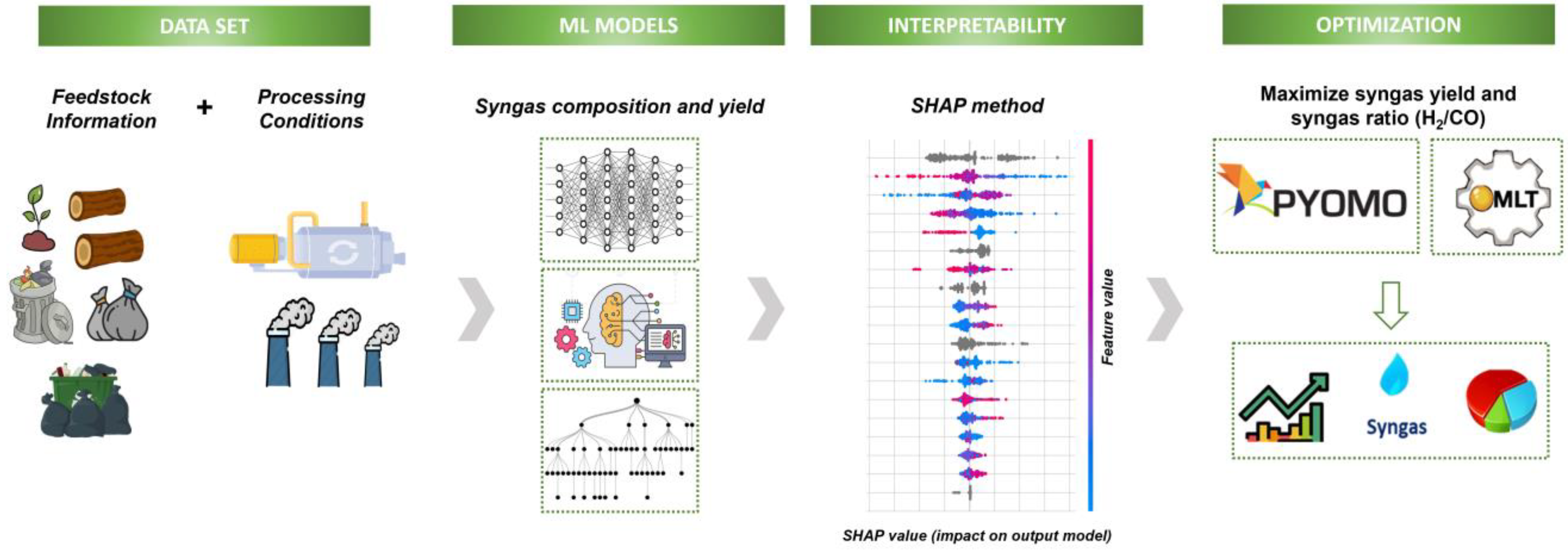
Figure 1. Schematic representation of the strategy proposed in this study.
Resources 14 00157 g001
Figure 2. Summary of the methodology used.
Resources 14 00157 g002
Figure 3. Heat map of variable correlation in syngas production.
Resources 14 00157 g003
Figure 4. Relationship between reactor type and syngas yield.
Resources 14 00157 g004
Figure 5. Predictions versus actual values of the best values calculated by the RNA model.
Resources 14 00157 g005
Figure 6. Impact of input variables on output variables N2, H2, CO, and syngas yield.
Resources 14 00157 g006aResources 14 00157 g006b
Figure 7. Impact of input variables on output variables CO2 and CH4.
Resources 14 00157 g007
Figure 8. Pareto curve between H2/CO ratio and syngas yield.
Resources 14 00157 g008
Figure 9. Compositions of H2 and CO for the different optimal solutions.
Resources 14 00157 g009
Table 1. Experimental data on biomass gasification.
MinMaxMeanSD
Feedstock information
TypePine sawdust, Woody biomass, Herbaceous biomass, Sewage sludge, Municipal solid waste, Other
ShapePellets, Fibers, Dust, Particles, Other
Particle Size (mm)0.2570.004.476.52
LHV [MJ/kg wb]11.5042.9018.486.43
Ultimate Analysis
C [%daf]40.0786.0351.318.83
H [%daf]3.7914.236.821.91
N [%daf]07.320.991.79
S [%daf]01.610.330.43
O [%daf]053.4039.9310.41
Proximate Analysis
Ash [%db]0.2744.006.8911.51
Moisture [%db]027.008.425.47
Volatile Matter [%db]56.0089.1177.758.72
Fixed carbon [%db]9.0723.8215.713.06
Lignocellulosic Composition
Cellulose [% db]29.6046.2038.845.15
Hemicellulose [%db]14.0029.6021.304.52
Lignin [%db]13.6033.0024.145.87
Gasifier Conditions and Information
Temperature [°C]553.001050.00796.0079.61
Operation ModeBatch, Continuous
Residence Time [min]1.93403.0087.7296.60
Steam/Biomass [wt/wt]0.004.041.090.76
ER0.090.870.290.10
Gasifying AgentAir, Air + Steam, Oxygen, Steam, Air + Oxygen, Other
Reactor TypeFluidized Bed, Fixed Bed, Circulating Fluidized Bed
Bed MaterialOlivine, Silica, Dolomite, Alumina, Olivine Sand, Calcium Oxide
CatalystPresent, Not present
ScaleLab, Pilot
Table 2. Summary of target variables.
MinMaxMeanSD
N2 [vol.%db]0.0074.9035.3827.04
H2 [vol.%db]3.0073.8522.4216.88
CO [vol.%db]2.2050.0020.1210.11
CO2 [vol.%db]0.0038.2516.286.21
CH4 [vol.%db]0.2517.005.323.43
C2Hn [vol.%db]09.502.091.48
Syngas yield [Nm3/kg wb]0.496.191.790.94
Table 3. Search space for the different hyperparameters of the models.
ModelHyperparameterVariable TypeMinMax
Random
Forest
BootstrapCategoricalTrue, False
Max featuresCategoricalNone, sqrt, log2
N estimatorsInteger10500
Max depthInteger224
Min samples splitInteger220
Min samples leafInteger120
CatBoostBootstrap typeCategoricalBayesian, Bernoulli, MVS
Learning rateFloat0.010.8
DepthInteger216
N estimatorsInteger10500
L2 leaf regFloat150
ANNHidden layersInteger16
Neurons per layerInteger12200
Learning RateLog1 × 10−51 × 10−1
Batch sizeInteger110
Regularization parameter (L2)Log1 × 10−41 × 10−1
Table 4. Optimal values found for each model.
ModelHyperparameterVariable TypeOptimal ValueAverage Time
Random
Forest
BootstrapCategoricalyes1 h
Max featuresCategorical-
N estimatorsInteger26
Max depthInteger14
Min samples splitInteger4
Min samples leafInteger1
CatBoostBootstrap typeCategorical-8 h
Learning rateFloat0.4348
DepthInteger4
N estimatorsInteger447
Reg hoja L2Float30.6249
ANNHidden layersInteger515 h
Neurons per layerInteger167
Integer16
Integer148
Integer35
Integer36
Learning RateLog0.0002
Batch sizeInteger6
Regularization parameter (L2)Log0.0003
Table 5. Mean ± standard deviation of performance metrics (RMSE, MAE, R2, and R var _ weighted 2 ) obtained from 5-fold cross-validation of the ANN model.
Output
Variables
RMSEMAER2 R var _ weighted 2
MeanStd (±)MeanStd (±)MeanStd (±)MeanStd (±)
N20.18060.06470.12070.77710.96380.02880.94400.0323
H20.24750.07260.17500.73470.93790.0241
CO0.34540.16460.24190.62460.87130.0707
CO20.37480.09260.26420.33410.85730.0634
CH40.38030.06680.25050.07750.83550.0430
C2Hn0.62750.17810.39700.07280.63170.1009
Syngas Yield0.28380.08730.20990.04900.91710.0458
Table 6. Results of the models in predicting N2, H2, CO, CO2, CH4, C2Hn, and syngas yield.
Model/MetricsRMSEMAEMAPER2
N2
 Random Forest0.03100.08450.15350.9704
 CatBoost0.01650.10250.14580.9843
 RNA0.01460.08710.17570.9860
H2
 Random Forest0.03040.12020.94080.9698
 CatBoost0.03300.13540.98320.9672
 RNA0.02970.11871.65010.9705
CO
 Random Forest0.08550.19492.43440.9149
 CatBoost0.06670.20111.96750.9335
 RNA0.062330.18571.67140.9380
CO2
 Random Forest0.08740.21071.43990.9016
 CatBoost0.11620.25321.44940.8692
 RNA0.10780.21141.86870.8787
CH4
 Random Forest0.27410.26400.35830.7557
 CatBoost0.19530.24800.35490.8258
 RNA0.19220.23430.35530.8286
C2Hn
 Random Forest0.47380.40180.82340.6190
 CatBoost0.47210.43000.78230.6204
 RNA0.50380.40220.72330.5949
Syngas Yield
 Random Forest0.10480.21850.79830.9181
 CatBoost0.10290.23951.34670.9197
 RNA0.06870.17461.06930.9463
Table 7. Optimal values obtained for the variables of solutions 1, 2, 6, 7, and 8.
Solution 1Solution 2Solution 6Solution 7Solution 8
Feed LHV11.514.7942.9042.9042.90
C40.7943.8144.9954.9152.43
H4.467.28314.2314.2314.23
N5.7425981.7460.000.4220.00
S0.7398730.2210.520.000.00
O0.0031.870.003.0124.92
Feed ash5.530.270.270.270.27
Feed moisture1.327.070.040.000.00
Feed VM88.7578.8389.1189.1189.11
Feed FC22.1516.949.209.079.07
Temperature928.12762.59925.56872.97813.46
Operating conditionContinuousContinuousContinuousContinuousContinuous
Steam/biomass ratio2.141.730.850.701.05
ER0.100.210.600.670.80
Gasifying agentAir + steamSteamSteamOtherOther
Reactor typeFixed bedFluidized bedFluidized bedFluidized bedFluidized bed
Bed materialCalcium oxideCalcium oxideCalcium oxideCalcium oxideDolomite
CatalystPresentPresentPresentPresentPresent
ScalePilotPilotPilotPilotPilot
H2/CO ratio19.4513.582.411.960.76
Yield (Nm3/wb)12678
Disclaimer/Publisher’s Note: The statements, opinions and data contained in all publications are solely those of the individual author(s) and contributor(s) and not of MDPI and/or the editor(s). MDPI and/or the editor(s) disclaim responsibility for any injury to people or property resulting from any ideas, methods, instructions or products referred to in the content.