Article

Elastic Wave Propagation in a Stainless-Steel Standard and Verification of a COMSOL Multiphysics Numerical Elastic Wave Toolbox

by
Mohsen Bazargan
1,2,3,*,
Bjarne S. G. Almqvist
1,
Hem Bahadur Motra
4,
Pooyan Broumand
5,
Tobias Schmiedel
1 and
Christoph F. Hieronymus
1
1
Department of Earth Sciences, Uppsala University, Villavägen 16, 752 36 Uppsala, Sweden
2
Rock Engineering, Geosigma Part of Rejlers, Sankt Eriksgatan 113, 113 43 Stockholm, Sweden
3
WSL Institute for Snow and Avalanche Research SLF, 7260 Davos Dorf, Switzerland
4
Institute for Geosciences, Christian Albert University of Kiel, 24118 Kiel, Germany
5
Department of Civil and Environmental Engineering, Shiraz University, Shiraz 1585-71345, Iran
*
Author to whom correspondence should be addressed.
Resources 2022, 11(5), 49; https://doi.org/10.3390/resources11050049
Submission received: 23 February 2022 / Revised: 9 May 2022 / Accepted: 11 May 2022 / Published: 17 May 2022

Abstract

:
Laboratory-based elastic wave measurements are commonly used to quantify the seismic properties of Earth’s crust and upper mantle. Different types of laboratory apparatuses are available for such measurements, simulating seismic properties at different pressure and temperature. To complement such laboratory measurements, we present a numerical toolbox to investigate the seismic properties of rock samples. The numerical model is benchmarked against experimental results from a multi-anvil apparatus, using measurements of a stainless steel calibration standard. Measured values of the mean compressional- and shear-wave velocities at room conditions of the steel block were 6.03 km/s and 3.26 km/s, respectively. Calculated numerical results predicted 6.12 km/s and 3.30 km/s for compressional and shear-wave velocities. Subsequently, we measured Vp and Vs up to 600 MPa hydrostatic confining pressure and 600 °C. These measurements, at pressure and temperature, were then used as the basis to predict numerical wave speeds. There is, in general, good agreement between measurement and predicted numerical results. The numerical method presented in this study serves as a flexible toolbox, allowing for the easy setup of different model geometries and composite materials.

1. Introduction

Seismic waves provide key geophysical observations on the structure and composition of Earth’s interior. Laboratory measurements provide the most direct constraints of seismic properties in rocks. Starting with the fundamental work of [1,2,3,4], laboratory measurements have explored a range of additional factors that influence elastic wave speed during the past 60 years, such as pressure and temperature [5,6,7,8,9,10,11], influence of micro-cracks e.g., [10], anisotropy e.g., [12,13,14,15], partial melt generation and its influence on seismic wave speed and attenuation [16,17,18,19,20,21,22,23].
As such, laboratory-derived elastic properties are invaluable for interpreting seismic data and provide an important method for investigating tectonic and geodynamic processes and understanding the inner Earth structure [7,24,25]. A complement to laboratory measurements are provided through predictive (e.g., effective medium) and numerical models e.g., [26,27,28,29,30,31,32,33,34]. Predictive and numerical experiments can help understand elastic wave propagation in a material by providing additional information to laboratory measurements. This is because models provide the possibility to investigate the effects of composition, structure, and geometry using inferences of the compositional e.g., [31,35] and structural characterization of materials e.g., [18,19,20,21,32,33,34,36]. We note that laboratory and numerical experiments are complementary and best used in combination.
In this study, the compressional (Vp) and shear wave (Vs) velocities of a near isotropic standard stainless steel were measured up to 600 MPa confining pressure and temperatures up to 600 °C using an ultrasonic frequency measurement setup in a multi-anvil apparatus. A numerical model created with the COMSOL Multiphysics® software was set up and benchmarked against the laboratory measurement data. COMSOL Multiphysics is a general-purpose commercial finite element software. Models were set up and tested in 2D and 3D to simulate elastic wave propagation in the multi-anvil apparatus for the same stainless steel standard in order to verify the model based on laboratory data. This numerical setup can be used as a toolbox to obtain a better understanding of the role of different features, ranging, for example, from microstructural effects of minerals in rocks to compositional layering at the macroscopic scale. In this study, the numerical benchmark models consider an elastic isotropic material with various boundary conditions.

2. Methodology

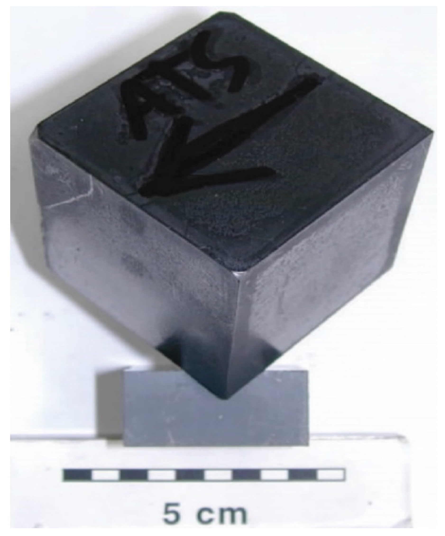
2.1. Sample Description

The sample is a homogenous cube of steel with edge lengths of 43 mm (Figure 1; steel grade ATS 314). The steel is composed mainly of Fe (~55–60%), with minor amounts of Cr (~25%), Ni (~20%), Mn (~2%), Si (~1–3%), and minor C, S, and P. The listed mechanical properties at room conditions show a modulus of elasticity (Young’s modulus, E) of 200 GPa and a density of 7900 kg/m3 (https://www.azom.com/article.aspx?ArticleID=8259, accessed on 4 March 2022).

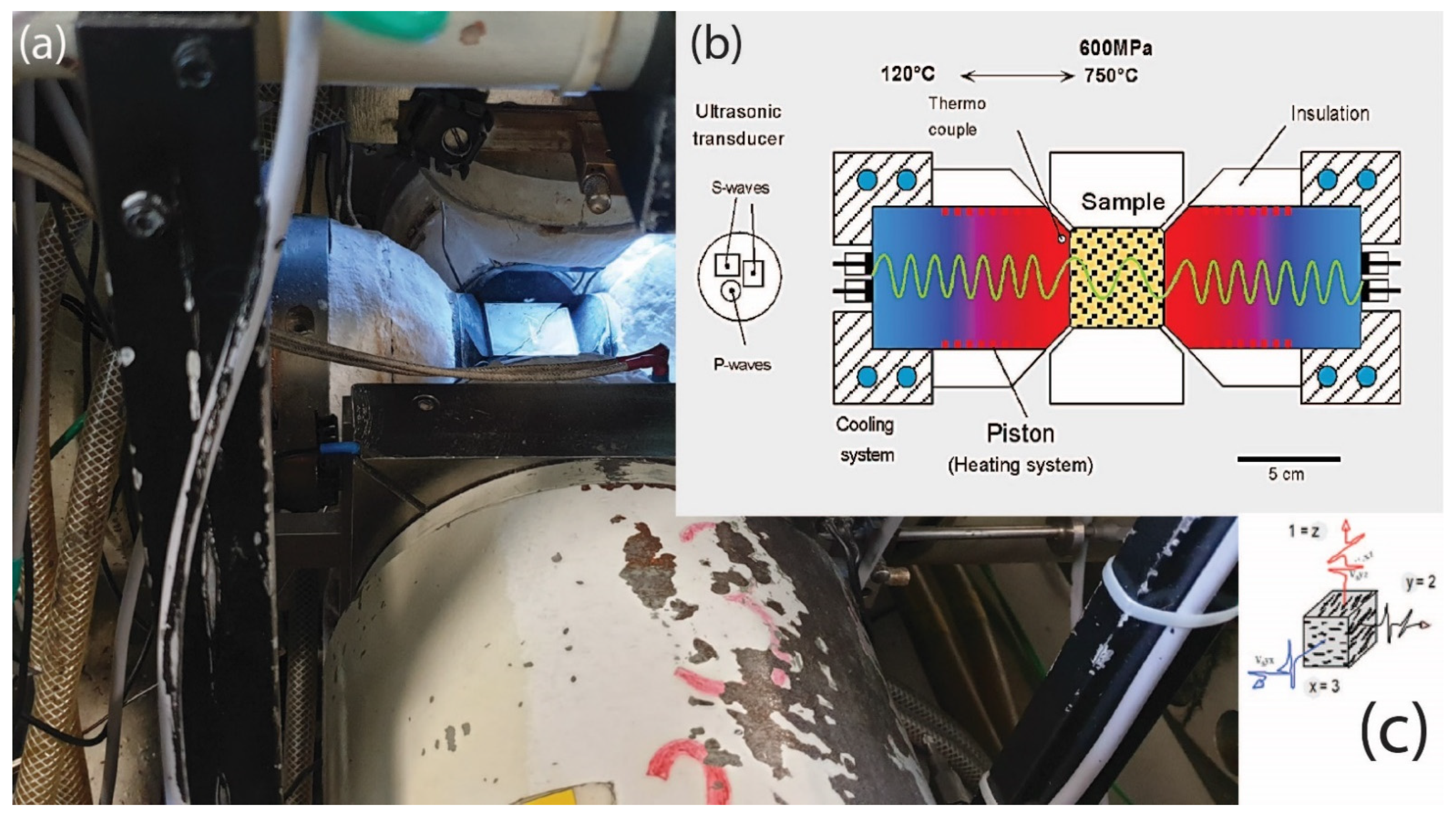
2.2. Experimental Setup

The laboratory measurements were performed with a triaxial multi-anvil apparatus (Figure 2) at the Institute for Geosciences at Kiel University, Germany. The apparatus has six pistons that are used to apply stresses. Ultrasonic velocities (P- and S-waves) were measured using the ultrasonic pulse transmission technique e.g., [1,2,6,8,9,10,11,12,13,14,15,36]. Three ultrasonic transducers were mounted at the end of each piston in a configuration that allows for the transmission of one compressional wave velocity, Vp, and two orthogonally polarized shear wave velocities, Vs1 and Vs2, along the three sample axes. The dominant frequencies of the transducers were 2 MHz and 1 MHz for P- and S-waves, respectively.
The apparatus is capable of operating at temperatures up to 750   ; however, in order to prevent the initiation of thermal cracks or the propagation of existing cracks with thermal-induced stresses, as a laboratory routine, the samples are generally tested to a maximum confining pressure of 600 MPa and a temperature up to 600 °C. Changes in sample dimensions, as a function of pressure and temperature, are monitored by linear strain sensors, which are used to correct Vp and Vs measurements. In the current study, the experiments began at room pressure and temperature conditions, followed by an incremental increase in pressure to 600 MPa. In the second phase, the confining pressure was kept constant, and the temperature was increased to 600 °C, in steps of 100 °C. During these two phases, when the apparatus reached the desired condition, ultrasonic wave pulses were applied to the sample along the three principal axes. V p and V s of the corresponding nine ultrasonic waves were measured along the three sample axes, three were P, and six were S waves.
The elastic wave speeds were calculated by the following equations:
Vp,s = L/Δtp,s
where L is the sample length (in m), Δt is the time of flight of the ultrasonic wave, measured in seconds. To compensate for the change in length at higher pressure and temperature conditions, the linear strain was used to recalculate the velocity, using:
Vp,s(P,T) = (L − ΔL)/Δtp,s
where ΔL represents the change in length of the sample, measured based on the piston displacement at elevated pressures and temperatures. Similarly, the density (ρ) of the sample is calculated based on the experimental condition, which at room conditions is:
ρ 0 = m V
where m is the sample mass (kg) and V is the sample volume (m3). Mass and volume were determined by measurements of weight and sample length, and since the sample is small, any influence due to gravity is neglected. At elevated pressure and temperature conditions, the change in volume (ΔV) is considered, and:
ρ ( P ,   T ) = m V Δ V
The first and second dynamic elastic moduli (Lamé’s constants, λ and µ) are calculated from the measured Vp and Vs, such that:
V p = 2 μ + λ ρ
V s = μ ρ
from which Young’s modulus (E) and the Poisson ratio (υ) can be calculated, according to:
E = μ ( 3 λ   + 2 μ ) λ   +   μ
ν = λ 2   ( λ   +   μ )
Finally, we also calculate the mean Vp and Vs, as well as the anisotropy of Vp (%AVp), using:
Vp   mean = V pmax + V pmin + V pint 3
% AVp = V pmax V pmin V pmean × 100
where Vpmax, Vpmin, and Vpint are the maximum, minimum, and intermediate P-wave velocities measured along the principal sample axes (Figure 2c). In addition, we calculated the difference in shear wave speed of the two polarized shear waves in terms of percentage (dVs%), using dVs (%) = (Vs1 + Vs2)/(Vs1 − Vs2) × 100 (%).
Measurements were carried out in two phases for increasing pressure and temperature. In the first phase of measurements, the ultrasonic wave velocities (Vp, Vs) were measured while the pressure was increased step-wise from the room conditions up to 600 MPa (Figure 3a,c,e,g). For each pressure increment, the sample was allowed to equilibrate at the new pressure for 5 min before the measurement was conducted. In the second phase, the confining pressure was kept constant at 600 MPa, and the temperature was increased step-wise to 600 °C (Figure 3b). A period of 30 min was used to let the sample equilibrate at the new temperature. The confining pressure was kept near-constant, at 600 MPa, to limit thermally induced stresses due to expansion and re-opening of pores, flaws, and micro-cracks in the sample while measuring the ultrasonic wave speeds (Figure 3b,d,f,h). Linear strains from all 3 sample axes were measured during confining pressure conditions from room pressure to 600 MPa and temperatures from room conditions up to 600 °C (Figure 4a,b). Linear strain measurements reflect sample volume changes because of increasing pressure and temperature. This volumetric change, calculated from the linear strain, indicates how the sample changes dimensions during pressurization and increase in temperature. The linear strain is small for the pressure increase and relatively much larger for an increase in temperature. In other words, the effect of temperature is significantly greater than the effect of pressurization in influencing the sample volume (Figure 4a,b). Figure 4c,d show the calculated Young’s modulus and Poisson ratio, from the Vp and Vs measurements, as a function of pressure and temperature. For further details on the laboratory measurement technique, we refer to [6,36].

2.3. Numerical Methodology

Governing Equations and Constitutive Laws

For a general solid in two and three dimensions, with boundary conditions in one to two dimensions and neglecting body force, the equation of motion can be expressed in Einstein notation as:
σ ij , j = ρ u · · i ;   for   i , j = 1 , 2 , 3
where σij is the stress tensor, ρ is density, and u i is the displacement vector. Dots above variables specify time derivatives. This equation is supplemented with suitable sets of boundary and initial conditions. For rheology applications, a pure linear elastic constitutive law (Hooke’s law) is used [37]:
E ( 1 + ν )   ( ν   ε kk   δ ij ( 1 2 ν ) + ε ij ) =   σ ij
In Equation (13), the isotropic form of Hooke’s law is given in terms of E and v; εij is the strain tensor, εαα is the volumetric strain, and δij is the Kronecker delta. The ε ij are also the infinitesimal strain tensor components which are kinematically related to the displacement field u i , as follows:
ε ij = 1 2 ( u i , j + u j , i )
In COMSOL Multiphysics software, version 6.0, the Solid Mechanics module part of the Structural Mechanics Module has implemented the weak form of the above sets of equations in the framework of the finite element method and can be efficiently used to describe the seismic wave propagation in a solid media that is modeled as an isotropic linear elastic media.
The 3D FE mesh used was tetrahedral. The model steps are given in microseconds due to the very high frequency (MHz) of the incident wave, and the size of the samples is given in meters (Figure 5). The edge boundary condition for the compressional wave is zero displacement in the normal direction and free slip in the direction parallel to the boundary. Symmetry and roller boundary conditions are both the same in two-dimensional. For the shear wave, the displacements perpendicular to the polarization direction are set to zero, whereas in the polarization direction, the corresponding stress is set to zero (that is, on the plane with normal motions, the normal stress is set to zero, and on the plane with shear motions, the associated shear stress is set to zero). The buffer zone (piston setup in the current model) is formed out of the same material as the steel samples tested for this bench-mark study.

3. Results

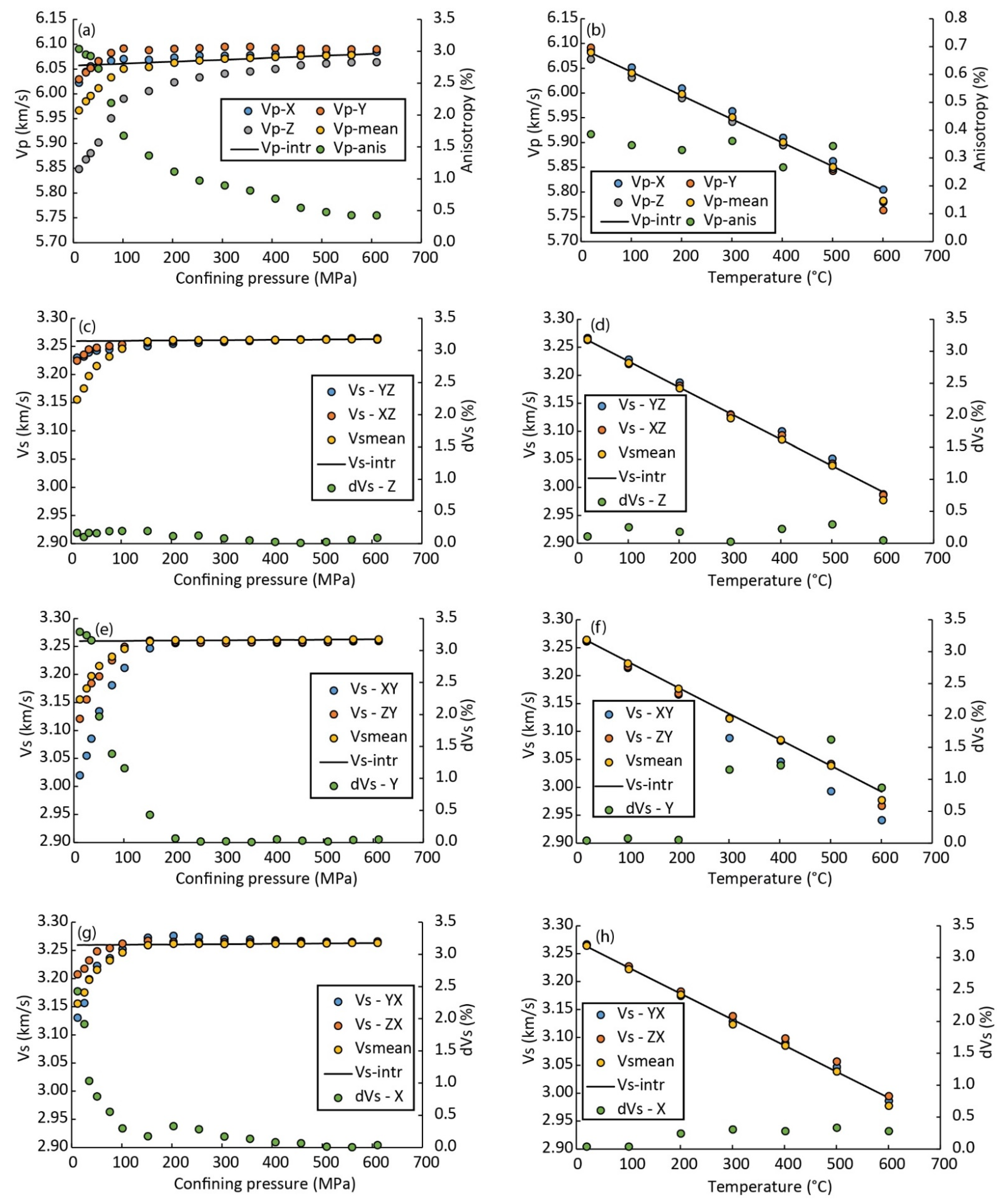
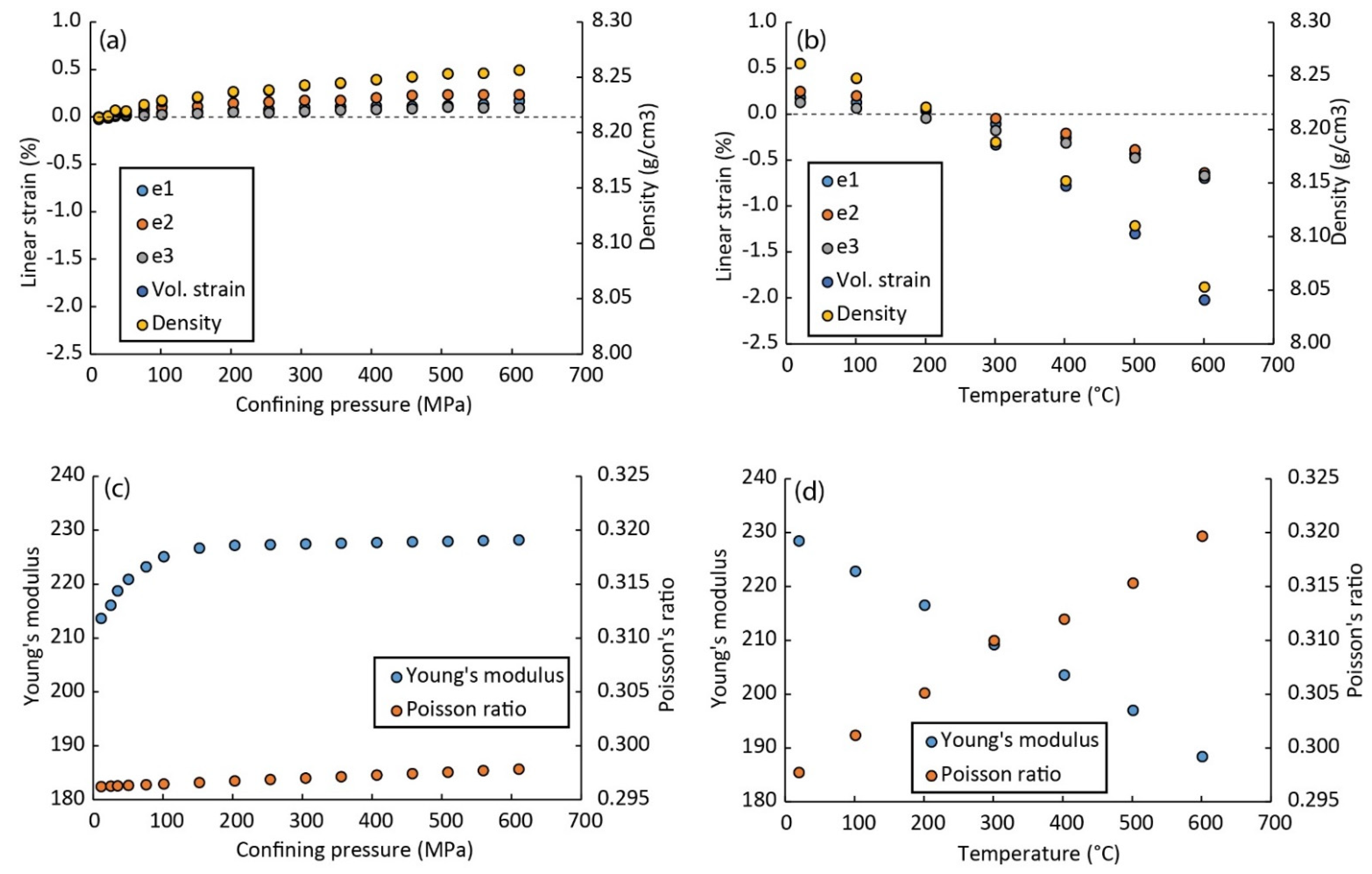
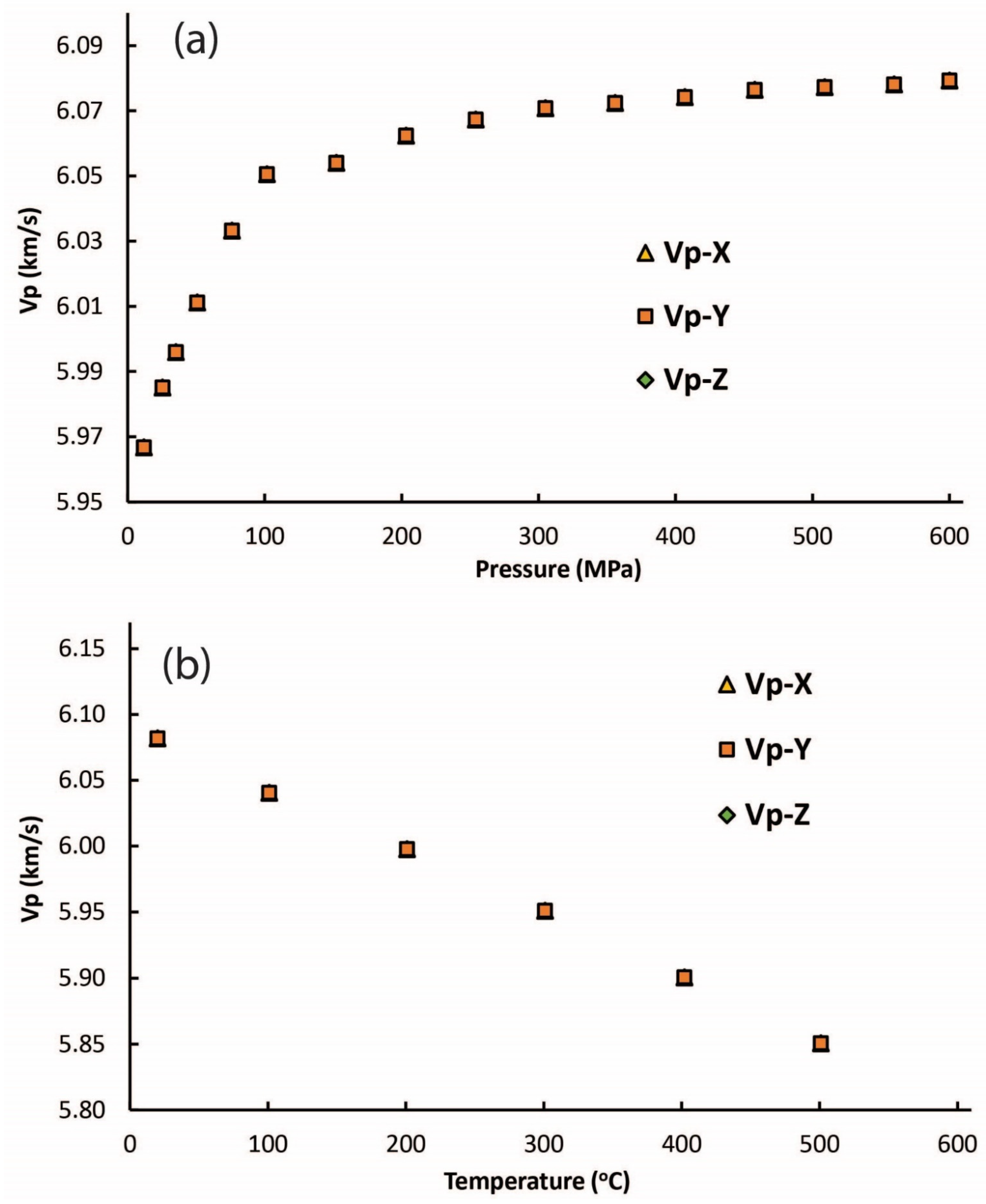
3.1. Laboratory Measurements of Ultrasonic Wave Velocities and Dynamic Elastic Properties

From the Vp and Vs measurements along sample X, Y and Z-axes, it was possible to obtain Vpmean and Vsmean (Equation (9)), as well as AVp, AVs (Equation (4)), and linear strain. Vpmean increased from 5.97 km/s to 6.08 km/s, from room pressure conditions to 600 MPa. The values of Vpmean decreased from 6.08 to 5.80 km/s during increasing temperature to 600 °C (Figure 3b). Anisotropy of Vp is below 1%, indicating that the steel can be considered effectively isotropic. The anisotropy increases slightly from temperatures of 500 °C to 600 °C but is still below 1%. The intrinsic Vp and Vs presented in Figure 3 represent linear fits to the mean Vp above 200 MPa for Vp and Vs as a function of pressure, whereas the intrinsic Vp and Vs as a function of temperature take into account all Vp and Vs measurements as a function of temperature.
Linear strain along the 3 sample axes (ε1, ε2, and ε3) was determined from the piston displacement and shows how the sample deforms as a function of pressure and temperature. Negative linear strain is considered as an expansion of the sample in the laboratory measurement, whereas positive strain is considered compaction of the sample. Importantly, these data provide changes in sample length, which are subsequently used to calculate Vp and Vs and recalculate density. Linear strain appears similar along all sample axes during pressurization, with somewhat higher positive values of ε2 (sample shortening along the y-axis), compared to ε1 and ε3. During increasing temperature, linear strain along all sample axes is very similar, with negative values (expansion) but higher relative values compared to linear strain during pressurization. This indicates that heating the steel has a larger influence on sample volume compared to the pressurization, and hence also on Vp and Vs. From the Vp, Vs measurements, the material properties, including Young’s modulus, Poisson’s ratio, and density, were calculated (Figure 4c,d). The elastic constants and density served as input parameters for the numerical modeling of Vp and Vs and benchmarking of the model.

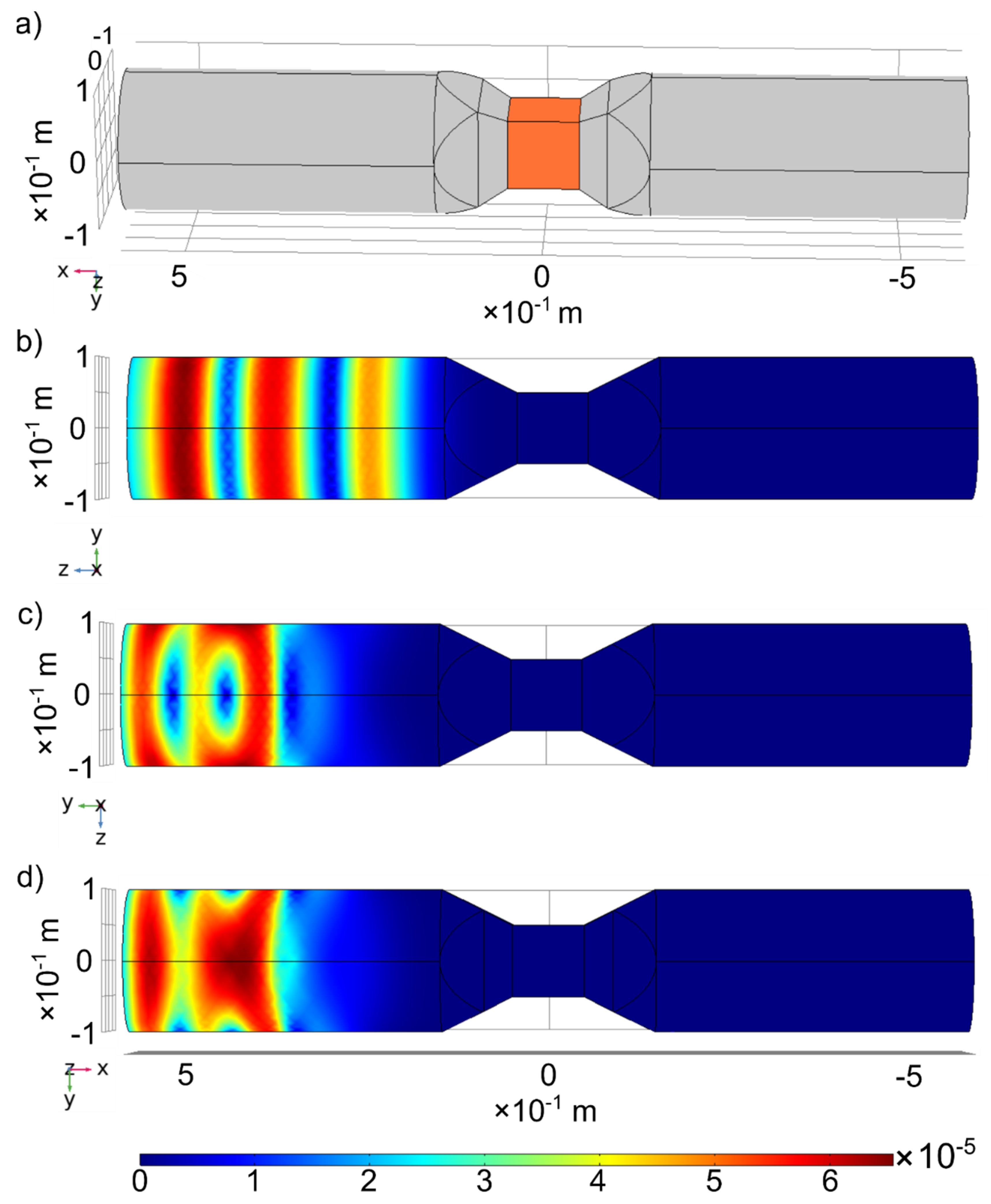
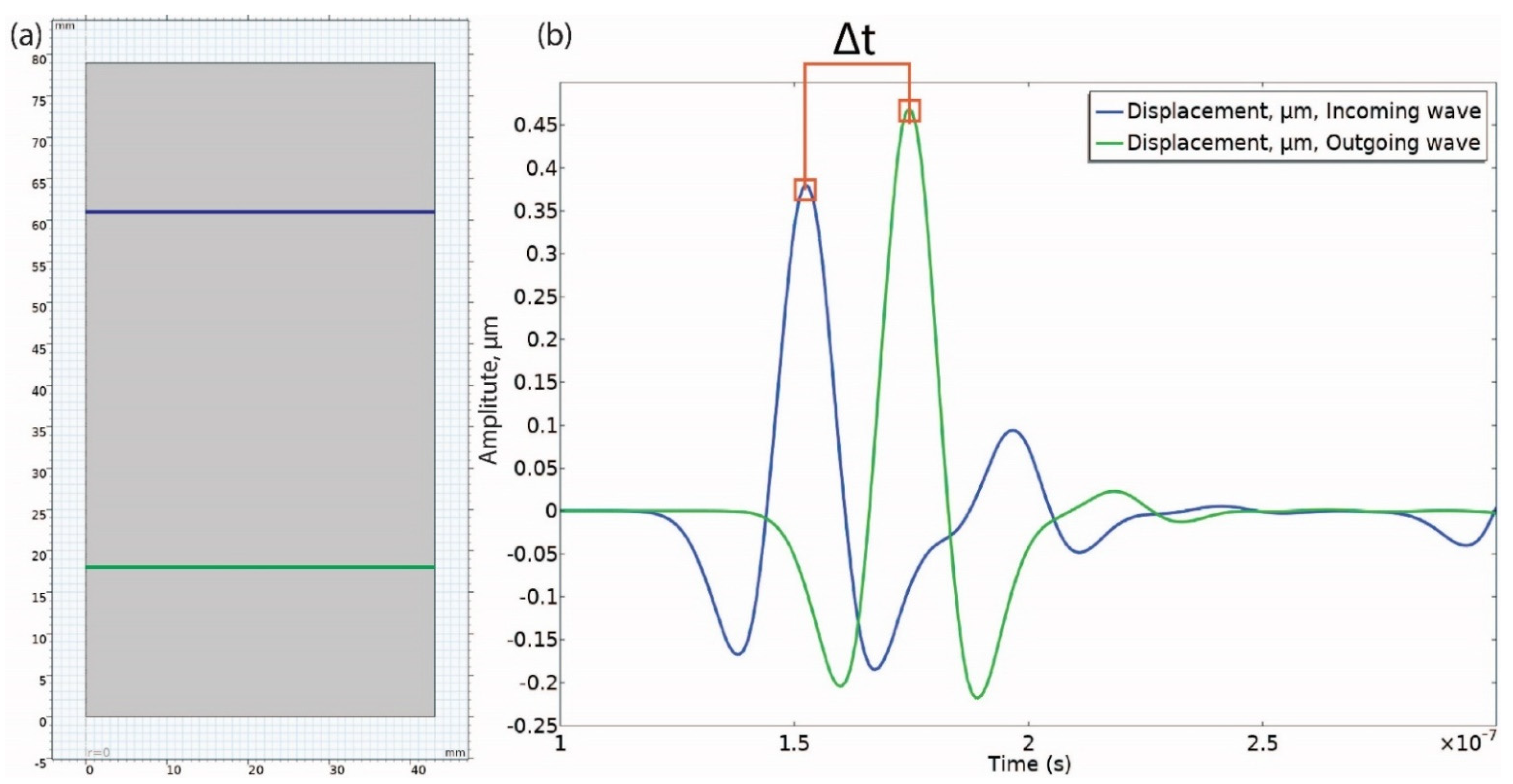
3.2. Numerical Modelling Results

The numerical models (used for benchmarking) were developed in two and three dimensions with the same material properties (Table 1) and similar geometry and boundary/initial conditions. The three-dimensional model is drawn to simulate a realistic setup of pistons and sample with similar dimensions used as in the laboratory (Figure 5). Since the geometry is symmetric, the extension from the two-dimensional case to the three-dimensional case is considered trivial, although it could be affected if different boundary conditions were used in the two different model setups. The geometry of the model, including the steel sample (in orange) in the middle and the pistons of the multi-anvil apparatus (in grey), are shown in Figure 5. Two buffer zones, representing the apparatus pistons, were placed on the left and right sides of the specimen to resemble the laboratory conditions as close as possible and eliminate model artifacts and edge effects as much as possible. Comparing the first peak arrival time of the incoming and outgoing waves of the constant geometry (in the sample), it is possible to calculate the Vp and Vs using Equation (1) from (Figure 6). The numerical test specimen was set up with material properties from Table 1.
The modeling results for two- and three-dimensional cases were essentially identical and differed by less than 2% in general compared to the laboratory measurements under all experimental conditions (Table 2). Even though it is expected that the measured and modeled Vp and Vs should perfectly coincide (given that the measured values are used as input for the models), the small difference likely arises from uncertainties in the picking of the modeled velocities and effects related to the setup of the model (e.g., size of the model mesh). In this model, the polarization is imposed as in Figure 5c,d. The polarized shear waves are equal for all two-dimensional cases, and no difference is observed in the S-waves for isotropic three-dimensional cases.
The density and elastic moduli of steel measurements make it possible to consider the influence of pressure and temperature effects on Vp and Vs in the numerical model (Figure 3 and Figure 4). The changes in density and elastic moduli during applied confining pressure were small, with ~2% change in density and ~5% change in elastic moduli from room pressure to 600 MPa. However, these changes were much more significant for increasing temperature (at a fixed confining pressure of 600 MPa), where density and Young’s modulus changed from 8256 kg/m3 and 228 GPa at room temperature to 8053 kg/m3 and 188 GPa at 600 °C (Figure 4c,d). Poisson’s ratio changed from 0.298 to 0.320 for the same increase in temperature. In the model, we use the recalculated density and elastic moduli to model Vp and Vs in order to incorporate the effect of pressure and temperature on elastic wave velocities. The numerical modeling results, presented in Figure 7 and in Table 2, generally illustrate no difference compared to the measured Vp and Vs. The models were ran as an isotropic elastic medium and therefore the models currently run very fast. However, more complicated models in three-dimensional geometries will have much longer run times than two-dimensional ones.

4. Discussion and Conclusions

This study presents a new COMSOL Multiphysics-based numerical model for elastic wave propagation in materials in two- and three-dimensions, which is verified (benchmarked) using the results from laboratory measurements of steel up to 600 MPa confining pressure and temperatures up to 600 °C. The numerical modeling results show less than a 2% difference with measured experimental values; there was no difference between results from two- and three-dimensional models.
Although the model presented in this study presents a relatively simple application, in which the velocities obtained are based on known laboratory-measured Vp and Vs as a function of pressure and temperature, there is considerable flexibility in setting up different kinds of models. For example, geometries with anisotropic minerals due to lattice preferred orientation, stratified geometry, grain size and shape and structural effects, such as inclusions of partial melting, the existence of microcracks, the effect of grain boundaries, and grain sliding. The advantage of the numerical model, developed in COMSOL Multiphysics, is the possibility to investigate elastic wave propagation in a variety of model setups, considering numerical experiments both on a laboratory scale and field scale (as well as upscaling of laboratory results). This numerical tool can include a variety of mineral arrangements (geometry) and can propagate P- and S-waves from different directions to determine seismic anisotropy; it is simple to extend investigations to study the directional dependency of waves and anisotropy into three dimensions. Three-dimensional models are valuable since all laboratory experiments are performed in three dimensions.
A notable effect in laboratory measurements is the closure of pores and microcracks during sample pressurization, which is illustrated by an exponential increase in elastic wave speed at low confining pressure, which generally occurs below 200 MPa e.g., [1,2,38,39,40]. In geological samples, this is known as the crack-closure domain, in which no notable contribution to sample volume change occurs (i.e., no notable linear strain changes), but with a pronounced effect on Vp and Vs. To incorporate such crack closure requires a modification of the numerical model but remains possible with the COMSOL Multiphysics software. In contrast, the effect of temperature on samples, which results in thermal expansion, is evident in linear strain measurements and associated sample volume change. An extension of the model can be set up to investigate the effects of pressure and temperature changes on Vp and Vs by incorporating thermal expansion and pressure/temperature-dependent derivatives of Vp and Vs.
Current numerical results allow studying the relations between the structural framework of the rocks (foliation, lineation), velocity anisotropy, shear wave splitting, and shear wave polarization. Anisotropic materials can be considered in the model using the complete elastic stiffness tensor (as defined by Hooke’s law in anisotropic form) with up to 21 independent elastic constants e.g., [29] (see appendix/online Supplementary Materials). Such a model setup can play an essential role when studying the influence of crystallographic preferred orientation (CPO) developed by viscoplastic deformation in ductile materials e.g., [16,17,24,25,26,27,28]. Data sets for CPOs can be obtained from measurements using Scanning Electron Microscope Electron Backscatter Diffraction or, for example, from viscoplastic self-consistent models e.g., [41,42]. Changes in the shape and sizes of geometrical inclusions can, for example, represent grain shape and size e.g., [6,36,43,44]), as such numerical models are used to further investigate the effect of grain sizes and grain boundary on ultrasonic waves. The numerical COMSOL Multiphysics model introduced in this study provides a relatively simple option to study the elastic properties of complex geological materials and serves as a useful addition in the fields of digital rock physics and materials science. Further information and examples of applications with the COMSOL Multiphysics model presented in this study are available in Supplementary Materials and the YouTube channel: https://youtu.be/XxCVrix54V4 (accessed on 20 February 2022).

Supplementary Materials

The following supporting information can be downloaded at: https://www.mdpi.com/article/10.3390/resources11050049/s1, S1: Numerical model setup for anisotropic medium; The module recipe used with this COMSOL model is freely available in Supplementary Materials and the YouTube channel https://youtu.be/XxCVrix54V4 (accessed on 20 February 2022)

Author Contributions

M.B. developed the concept for this study. Manuscript was written by M.B. and B.S.G.A. with help from T.S. and P.B., Numerical modeling was performed by M.B. with suggestions from C.F.H., P.B. and B.S.G.A. Laboratory experiments were performed by H.B.M. All authors have read and agreed to the published version of the manuscript.

Funding

This research was funded by Uppsala Universitet Geologiska Sektionen, grant date April 2020. The authors acknowledge the Swedish Research Council for the financial support through the project 2018-03414, awarded to B. Almqvist.

Institutional Review Board Statement

Not applicable.

Informed Consent Statement

Not applicable.

Data Availability Statement

Not applicable.

Conflicts of Interest

The authors declare no conflict of interest.

References

  1. Birch, F. The velocity of compressional waves in rocks to 10 kilobars: 1. J. Geophys. Res. Earth Surf. 1960, 65, 1083–1102. [Google Scholar] [CrossRef]
  2. Birch, F. The velocity of compressional waves in rocks to 10 kilobars: 2. J. Geophys. Res. Earth Surf. 1961, 66, 2199–2224. [Google Scholar] [CrossRef]
  3. Christensen, N.I. Compressional wave velocities in metamorphic rocks at pressures to 10 kilobars. J. Geophys. Res. Earth Surf. 1965, 70, 6147–6164. [Google Scholar] [CrossRef]
  4. Christensen, N.I. Elasticity of ultrabasic rocks. J. Geophys. Res. 1966, 71, 5921–5931. [Google Scholar] [CrossRef]
  5. Bazargan, M.; Broumand, P.; Motra, H.; Almqvist, B.; Hieronymus, C.; Piazolo, S. A Numerical Toolbox to Calculate the Seismic Properties of Micro Sized Isotropic and Anisotropic Minerals. In Proceedings of the Mineral Exploration Symposium, Virtual Event, 17–18 September 2020; pp. 1–3. [Google Scholar] [CrossRef]
  6. Bazargan, M.; Motra, H.B.; Almqvist, B.; Piazolo, S.; Hieronymus, C. Pressure, temperature and lithological dependence of seismic and magnetic susceptibility anisotropy in amphibolites and gneisses from the central Scandinavian Caledonides. Tectonophysics 2021, 820, 229113. [Google Scholar] [CrossRef]
  7. Christensen, N.I. Compressional wave velocities in rocks at high temperatures and pressures, critical thermal gradients, and crustal low-velocity zones. J. Geophys. Res. Earth Surf. 1979, 84, 6849–6857. [Google Scholar] [CrossRef]
  8. Kern, H.; Burlini, L.; Ashchepkov, I. Fabric-related seismic anisotropy in upper-mantle xenoliths: Evidence from measurements and calculations. Phys. Earth Planet. Inter. 1996, 95, 195–209. [Google Scholar] [CrossRef]
  9. Kern, H.; Gao, S.; Liu, Q.-S. Seismic properties and densities of middle and lower crustal rocks exposed along the North China Geoscience Transect. Earth Planet. Sci. Lett. 1996, 139, 439–455. [Google Scholar] [CrossRef]
  10. Kern, H. Measuring and Modeling of P- and S-Wave Velocities on Crustal Rocks: A Key for the Interpretation of Seismic Reflection and Refraction Data. Int. J. Geophys. 2011, 2011, 530728. [Google Scholar] [CrossRef] [Green Version]
  11. Scheu, B.; Kern, H.; Spieler, O.; Dingwell, D. Temperature dependence of elastic P- and S-wave velocities in porous Mt. Unzen dacite. J. Volcanol. Geotherm. Res. 2006, 153, 136–147. [Google Scholar] [CrossRef]
  12. Kern, H.; Popp, T.; Gorbatsevich, F.; Zharikov, A.; Lobanov, K.; Smirnov, Y. Pressure and temperature dependence of VP and Vs in rocks from the superdeep well and from surface analogues at Kola and the nature of velocity anisotropy. Tectonophysics 2001, 338, 113–134. [Google Scholar] [CrossRef]
  13. Kern, H. The effect of high temperature and high confining pressure on compressional wave velocities in quartz-bearing and quartz-free igneous and metamorphic rocks. Tectonophysics 1978, 44, 185–203. [Google Scholar] [CrossRef]
  14. Kern, H. Effect of high-low quartz transition on compressional and shear wave velocities in rocks under high pressure. Phys. Chem. Miner. 1979, 4, 161–171. [Google Scholar] [CrossRef]
  15. Kern, H.; Tubia, J. Pressure and temperature dependence of P- and S-wave velocities, seismic anisotropy and density of sheared rocks from the Sierra Alpujata massif (Ronda peridotites, Southern Spain). Earth Planet. Sci. Lett. 1993, 119, 191–205. [Google Scholar] [CrossRef]
  16. Almqvist, B.; Cyprych, D.; Piazolo, S.; Bazargan, M. Contributions of microstructure and crystallographic preferred orientation to seismic anisotropy in the lower continental crust, European Geoscience Union. In Proceedings of the EGU General Assembly Conference, Vienna, Austria, 8–13 April 2018; p. 13249. [Google Scholar]
  17. Almqvist, B.S.; Cyprych, D.; Piazolo, S. Seismic anisotropy of mid crustal orogenic nappes and their bounding structures: An example from the Middle Allochthon (Seve Nappe) of the Central Scandinavian Caledonides. Tectonophysics 2021, 819, 229045. [Google Scholar] [CrossRef]
  18. Bazargan, M.; Almqvist, B.S.G.; Hieronymus, C.; Piazolo, S. Employing Finite Element Method using COMSOL multiphysics to predict seismic velocity and anisotropy: Application to lower crust and upper mantle rocks. In Proceedings of the 20th EGU General Assembly, EGU2018, Vienna, Austria, 4–13 April 2018; European Geoscience Union: Munich, Germany, 2018; p. 17139. [Google Scholar]
  19. Bazargan, M.; Almqvist, B.S.G.; Hieronymus, C.; Piazolo, S. Experimental investigation and numerical modelling of elastic wave propagation in meta-morphic rocks. In In Proceedings of the IGSC 2019, Uppsala, Sweden, 21–24 October 2019. [Google Scholar]
  20. Bazargan, M.; Hem, M.B.; Almqvist, B.S.G.; Hieronymus, C.; Piazolo, S. Elastic wave anisotropy in amphibolites and paragneisses from the Swedish Caledonides measured at high pressures (600 MPa) and temperatures (600 °C). In Proceedings of the 21th EGU General Assembly, EGU2019, Vienna, Austria, 7–12 April 2018; European Geoscience Union: Munich, Germany, 2019; p. 14397. [Google Scholar]
  21. Bazargan, M.; Hem, M.B.; Almqvist, B.S.G.; Hieronymus, C.; Piazolo, S. Numerical and Experimental Investigations of Elastic Wave Anisotropy in Monomineral and Polymineral Rocks, In Proceedings of the EGU 2020, Vienna, Austria, 3–8 May 2020.
  22. Ferri, F.; Burlini, L.; Cesare, B.; Sassi, R. Seismic properties of lower crustal xenoliths from El Hoyazo (SE Spain): Experimental evidence up to partial melting. Earth Planet. Sci. Lett. 2007, 253, 239–253. [Google Scholar] [CrossRef]
  23. Hughes, D.S.; Maurette, C. Variation of elastic wave velocities in basic igneous rocks with pressure and temperature. Geophysics 1957, 22, 23–31. [Google Scholar] [CrossRef]
  24. Almqvist, B.S.; Misra, S.; Klonowska, I.; Mainprice, D.; Majka, J. Ultrasonic velocity drops and anisotropy reduction in mica-schist analogues due to melting with implications for seismic imaging of continental crust. Earth Planet. Sci. Lett. 2015, 425, 24–33. [Google Scholar] [CrossRef]
  25. Almqvist, B.S.G.; Mainprice, D. Seismic properties and anisotropy of the continental crust: Predictions based on mineral texture and rock microstructure. Rev. Geophys. 2017, 55, 367–433. [Google Scholar] [CrossRef] [Green Version]
  26. Mainprice, D. A FORTRAN program to calculate seismic anisotropy from the lattice preferred orientation of minerals. Comput. Geosci. 1990, 16, 385–393. [Google Scholar] [CrossRef]
  27. Mainprice, D.; Bachmann, F.; Hielscher, R.; Schaeben, H.; Lloyd, G. Calculating anisotropic piezoelectric properties from texture data using the MTEX open source package. Geol. Soc. Spéc. Publ. 2014, 409, 223–249. [Google Scholar] [CrossRef] [Green Version]
  28. Mainprice, D. Seismic anisotropy of the deep Earth from a mineral and rock physics perspective. In Treatise in Geophysics, 2nd ed.; Schubert, G., Ed.; Elsevier: Oxford, UK, 2015; Volume 2, pp. 487–539. [Google Scholar]
  29. Mavko, G.; Mukerji, T.; Dvorkin, J. The Rock Physics Handbook, 3rd ed.; Cambridge University Press: Cambridge, UK, 2020. [Google Scholar] [CrossRef]
  30. Vel, S.S.; Cook, A.C.; Johnson, S.; Gerbi, C. Computational homogenization and micromechanical analysis of textured polycrystalline materials. Comput. Methods Appl. Mech. Eng. 2016, 310, 749–779. [Google Scholar] [CrossRef] [Green Version]
  31. Valcke, S.L.; Casey, M.; Lloyd, G.E.; Kendall, J.-M.; Fisher, Q.J. Lattice preferred orientation and seismic anisotropy in sedimentary rocks. Geophys. J. Int. 2006, 166, 652–666. [Google Scholar]
  32. Zhong, X.; Frehner, M.; Kunze, K.; Zappone, A. A novel EBSD-based finite-element wave propagation model for investigating seismic anisotropy: Application to Finero Peridotite, Ivrea-Verbano Zone, Northern Italy. Geophys. Res. Lett. 2014, 41, 7105–7114. [Google Scholar] [CrossRef] [Green Version]
  33. Zhong, X.; Frehner, M.; Kunze, K.; Zappone, A.S. A numerical and experimental investigation on seismic anisotropy of Finero peridotite, Ivrea-Verbano Zone, Northern Italy. IOP Conf. Series Mater. Sci. Eng. 2015, 82, 12072. [Google Scholar] [CrossRef] [Green Version]
  34. Walsh, J.B. The effect of cracks on the compressibility of rock. J. Geophys. Res. Earth Surf. 1965, 70, 381–389. [Google Scholar] [CrossRef]
  35. Naus-Thijssen, F.M.J.; Goupee, A.J.; Vel, S.S.; Johnson, S. The influence of microstructure on seismic wave speed anisotropy in the crust: Computational analysis of quartz-muscovite rocks. Geophys. J. Int. 2011, 185, 609–621. [Google Scholar] [CrossRef]
  36. Bazargan, M.; Almqvist, B.G.; Motra, H.B.; Klein, L.; Broumand, P.; Schmiedel, T.; Piazolo, S.; Hieronymus Ch, F. (In-Review), An Experimental and Numerical Investigation of Grain Size Effects on Ultrasonic Wave Velocities in Gabbro. Available online: https://www.diva-portal.org/smash/record.jsf?pid=diva2%3A1644695&dswid=-5596 (accessed on 10 May 2022).
  37. Malvern, L. Introduction to the Mechanics of a Continuous Medium; Prentice-Hill: Englewood Cliffs, NJ, USA, 1969. [Google Scholar]
  38. Wyllie, M.R.J.; Gregory, A.R.; Gardner, L.W. Elastic wave velocities in heterogeneous and porous media. Geophys. Soc. Explor. Geophys. 1956, 21, 41–70. [Google Scholar] [CrossRef]
  39. Wyllie, M.R.J.; Gregory, A.R.; Gardner, G.H.F. An experimental investigation of factors affecting elastic wave velocities in porous media. Geophysics 1958, 23, 459–493. [Google Scholar] [CrossRef]
  40. Takei, Y. Effects of Partial Melting on Seismic Velocity and Attenuation: A New Insight from Experiments. Annu. Rev. Earth Planet. Sci. 2017, 45, 447–470. [Google Scholar] [CrossRef]
  41. Lebensohn, R.A.; Maudlin, P.J.; Tomé, C.N. Viscoplastic Selfconsistent Modelling of the Anisotropic Behavior of Voided Polycrystals. AIP Conf. Proc. 2004, 712, 1771–1776. [Google Scholar] [CrossRef]
  42. Tome, C.; Lebensohn, R.A. Material Modeling with the Visco-Plastic Self-Consistent (VPSC) Approach: Theory and Practical Applications, 1st ed.; Elsevier: Amsterdam, The Netherlands, 2022; ISBN 9780128207130. [Google Scholar]
  43. Kim, D.; Lekić, V.; Ménard, B.; Baron, D.; Taghizadeh-Popp, M. Sequencing seismograms: A panoptic view of scattering in the core-mantle boundary region. Science 2020, 368, 1223–1228. [Google Scholar] [CrossRef] [PubMed]
  44. Lebedev, T.S.; Burtnij, P.A.; Korčin, V.A. Behaviour of the pore space in Gabbros and its relationship with elastic wave velocities and high pressures. Gerl. Beitr. Z. Geophys. S. 1974, 83, 170–180. [Google Scholar]
Figure 1. Standard stainless steel sample, ATS-314. The arrow mark on the sample shows the orientation of how the sample is placed in the multi-anvil apparatus.
Resources 11 00049 g001
Figure 2. (a) Setup of the multi-anvil apparatus and positioning of the P and S wave transducers. (b) Transducers are placed at the end of pistons, and thermocouples are placed close to the piston-sample interface, and (c) measurement setup along the three principal axes, X, Y, and Z (modified from [10]).
Resources 11 00049 g002
Figure 3. Ultrasonic Vp and Vs measured as a function of confining pressure and temperature from room conditions up to 600 MPa and 600 °C. (a) Vp as a function of confining pressure. Note that Vp is slower along the Z-axis than along X- and Y-axes at low confining pressure; the difference becomes very small at higher pressures. (b) Vp as a function of temperature at a fixed confining pressure (600 MPa). (c,e,g) show the measurements of two polarized shear waves and the shear wave splitting, dVs (%) as a function of confining pressure; (d,f,h) show the measurements of two polarized shear waves and the shear wave splitting, dVs (%) as a function of temperature.
Resources 11 00049 g003
Figure 4. (a) Linear strain as a function of confining pressure, along the different sample axes (e1, e2, and e3), as well as the volumetric strain; change in density is calculated based on the change in linear strain. (b) Linear strain and density as a function of temperature. (c,d) Calculated Young’s modulus and Poisson’s ratio (from the mean V p and V s ) as a function confining pressure and temperature, respectively.
Resources 11 00049 g004
Figure 5. Numerical model of three-dimensional steel specimen; the model is based on the isotropic material behavior, (a) model geometry, (b) compressional wave result, (c) shear wave with horizontal polarization, (d) shear wave vertical polarization. Calculated Vp and Vs from the model is presented in Table 1.
Resources 11 00049 g005
Figure 6. Illustration showing how the velocity is calculated from the incoming and outgoing waves; (a) geometry of investigation and the two sensor boundaries for the elastic wave (in blue and green), (b) waveform, where Δt is the time of flight-of-flight, determined from the peak amplitudes in the two waveforms.
Resources 11 00049 g006
Figure 7. Vp calculations from the two- and three-dimensional numerical modeling with COMSOL, investigating the effect of (a) pressure and (b) temperature on the elastic wave speed. Note that the models do not consider the changes in linear strain, but do take into consideration dynamic elastic moduli (Young’s modulus and Poisson ratio) and density. In contrast, the Vp and Vs laboratory measurements depend on the time-of-flight of the elastic wave and the change in sample length.
Resources 11 00049 g007
Table 1. Young’s modulus, Poisson’s ratio, and density for the laboratory measurements (used as input for the numerical model) and the output results in the form of the P wave and a shear wave (note that no polarization is reported in the numerical model).
Young’s Modulus (GPa)Poisson’s RatioDensity (kg/m3)Vp (km/s)Vs (km/s)
Laboratory experiment2280.29882566.033.26
Numerical results 2D/3D2280.29882566.13.3
Table 2. Laboratory measurements, numerical modeling, and their Vp data. Abbreviations: Temp—temperature (°C); Pc—Confining pressure; VpL—laboratory-measured Vp; VpN—numerically modeled Vp. Vpmean are calculated from laboratory measurements using Equation (9).
LaboratoryNumericaldVp (VpL-VpN)
Temp.PcVp-ZVp-YVp-XVp-ZVp-YVp-XdVp-ZdVp-YΔVp-XVp Mean
(°C)(MPa)(km/s)(km/s)(km/s)(km/s)(km/s)(km/s)(km/s)(km/s)(km/s)(km/s)
20125.856.036.025.9675.9675.967−0.120.060.065.967
20255.876.046.045.9855.9855.985−0.120.060.065.985
20355.886.056.065.9965.9965.996−0.120.060.065.996
20515.96.076.076.0116.0116.011−0.110.050.056.011
20765.956.086.076.0336.0336.033−0.080.050.036.033
201025.996.096.076.0516.0516.051−0.060.040.026.051
201526.016.096.076.0546.0546.054−0.050.030.016.054
202036.026.096.076.0626.0626.062−0.040.030.016.062
202546.036.096.086.0676.0676.067−0.030.020.016.067
203056.046.096.086.0716.0716.071−0.030.020.016.071
203566.056.096.086.0726.0726.072−0.030.0206.072
204076.056.096.086.0746.0746.074−0.020.020.016.074
204586.066.096.086.0766.0766.076−0.020.0106.076
205096.066.096.086.0776.0776.077−0.020.0106.077
205606.066.096.086.0786.0786.078−0.010.0106.078
206006.066.096.086.0796.0796.079−0.020.010.016.079
206006.076.096.096.0826.0826.082−0.010.0106.082
1016006.036.046.056.046.046.04−0.0100.016.04
2016005.995.996.015.9985.9985.998−0.0100.015.998
3016005.945.955.965.9515.9515.951−0.0100.015.951
4026005.895.95.915.9015.9015.901−0.0100.015.901
5016005.855.845.865.8515.8515.8510−0.010.015.851
6016005.785.765.85.7835.7835.7830−0.020.025.783
Publisher’s Note: MDPI stays neutral with regard to jurisdictional claims in published maps and institutional affiliations.

