Implementing Adaptive Voltage Over-Scaling: Algorithmic Noise Tolerance vs. Approximate Error Detection

Abstract

Adaptive Voltage Over-Scaling can be applied at run-time to reach the best tradeoff between quality of results and energy consumption. This strategy encompasses the concept of timing speculation through some level of approximation. How and on which part of the circuit to implement such approximation is an open issue. This work introduces a quantitative comparison between two complementary strategies: Algorithmic Noise Tolerance and Approximate Error Detection. The first implements a timing speculation by means approximate computing, while the latter exploits a more sophisticated approach that is based on the approximation of the error detection mechanism. The aim of this study was to provide both a qualitative and quantitative analysis on two real-life digital circuits mapped onto a state-of-the-art 28-nm CMOS technology.

1. Introduction

Energy efficiency is one of the main design concerns for today’s digital Integrated Circuits (ICs). This is true not only for portable applications, where the energy budget is limited by the use of thin batteries [1,2], but also for high-performance applications where a proper resource management improves sustainability at a large scale [3,4].

Classical micro-architectural and logic-level low-power techniques proposed in the past as a solution to break the power-wall, e.g., Dynamic Voltage Frequency Scaling [5,6,7], Body-Biasing [8], Multi-threshold CMOS (MTCMOS) [9,10], can improve energy efficiency only marginally. The weakness lies under their intrinsic “always-correct” nature, which dictates a theoretic lower bound of the energy savings. Let us take a straightforward implementation of voltage scaling for instance. There is a minimum supply voltage $Vd{d}_{min}$ at which timing paths violate the set-up time; below such threshold, timing faults arise and logic errors propagate. A further reduction of the $Vdd$ can m only be accomplished with modification of the circuit, e.g., reshaping the paths distribution via gate re-sizing [11] and/or timing-driven Boolean restructuring [12], or a relaxing of the timing constraint, e.g., by frequency scaling. Both solutions might have a negative impact on the energy efficiency. The former may induce overhead that overwhelms the savings brought by $Vdd$ lowering, especially when process variations come into play. The latter induces larger latency, which in turn may increase the overall energy consumption.

To address these drawbacks, techniques related to better-than-worst designs have been introduced, which propose Timing Speculation as a viable solution [13,14]. Their basic assumption, mainly a probabilistic one, is that only a small and infrequent sub-set of input patterns sensitize the longest timing paths; for $Vdd$ below $Vd{d}_{min}$, those paths are rarely activated therefore and timing faults remain latent. In the event they get excited, latent faults become true faults but the resulting error can be recovered through some correction mechanism. As a result, the circuit operates with minimal energy consumption for most of the time. Commonly referred to as “detect-and-correct”, this speculative approach has been extensively investigated in previous works (e.g., [15,16,17,18]).

The most practical implementation, called Razor, makes use of in-situ timing monitors that check the timing behavior of the circuit at run-time. The logic errors are always corrected to guarantee functionality, e.g., using instruction reply if the architecture is micro-instructed, while the error rate is used as feedback to the power management unit. Error-rate below a given threshold $E_{th}$ implies the availability of some margin for scaling down the $Vdd$. Error-rate larger than $E_{th}$ forces $Vdd$ to raise up in order to mitigate the overhead due to error correction. The result is an Adaptive Voltage Over-Scaling (AVOS) mechanism that evolves towards the minimum energy point. As reported in [19,20], substantial energy savings can be achieved depending on the circuit and its actual workload.

Recent advances in the field of energy-efficient ICs foresee the use of even more aggressive timing speculations [21]. The idea is straightforward, yet efficient: leverage the intrinsic property of error resilient applications, such as audio/video processing, where a degradation of the output quality does not affect the quality perceived by the user. The AVOS mechanism, such as the one implemented by Razor, may settle to lower $Vdd$, hence lower energy consumption, if errors are tolerated. Intuitively, energy and quality can be traded to meet the requirements.

The literature presents plenty of Energy–Quality scaling techniques. Although they are all tagged with the label Approximate, they show substantial differences. For instance, Algorithm Noise Tolerance (ANT) [22,23] and Approximate Error Detection-Correction (AED-C) [24] are two representative examples that stand at the opposite corners. They differ for the granularity at which they are applied and the kind of monitoring strategy adopted. The ANT applies at the architectural level implementing a direct measure of the error induced by the voltage scaling. The output produced by an approximated replica of the original circuit (commonly obtained by precision scaling) is compared with the output of the main circuit; the difference drives the voltage scaling. The AED-C applies at the circuit level instead and, similar to Razor, implements an indirect measure of output quality. More precisely, a Tunable Error-Detection mechanism (TunED) [25] is deployed to regulate the fault coverage; TunED allows reducing (increasing) the number of detectable faults and hence to accelerate (slow-down) the voltage scaling accordingly leading the output to lower (higher) quality. The difference between the two strategy is significant: while ANT approximates the computation, AED-C approximates the monitoring. This aspect is paramount as it gives the two approaches a complementary behavior that was deeply investigated in this study.

The broad objective of this work was to provide a fair comparison between ANT and AED-C. A parametric characterization conducted over a set of realistic applications quantified several figures of merit, e.g., energy savings, performance and area overhead. The benchmarks consisted of two digital filters, a FIR and a IIR, both synthesized and mapped onto a commercial FD-SOI CMOS technology at 28 nm. The FIR is a pipelined 16th-order low-pass filter in the direct form (12-bit in, 24-bit out) synthesized to f${}_{clk}$ = 650 MHz. The IIR is a pipelined 8th-order low-pass filter in direct form I (16-bit in, 32-bit out) synthesized to f${}_{clk}$ = 650 MHz. The results collected for a sequence of three different classes of baseband audio signals empirically disclose the efficiency of ANT and AED-C, also providing an assessment of the resulting energy–quality tradeoff.

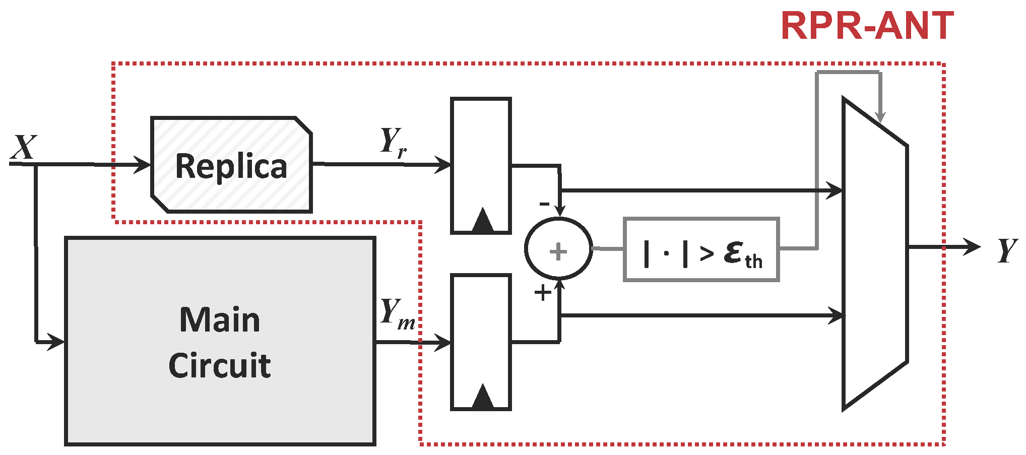
2. Algorithmic Noise Tolerance (ANT) via Reduced Precision Redundancy (RPR)

2.1. Implementation

The basic principle underlying the ANT technique is to accept errors as long as the output degradation due to $Vdd$ scaling remains below a given noise threshold [26,27]. As depicted in Figure 1, a typical ANT architecture consists of the main circuit coupled with its own lightweight replica, known in the literature as Reduced Precision Replica (RPR).

Such replica is approximated through arithmetic precision scaling, namely dropping some of the LSBs and it serves as ground reference for the assessment of the output quality of the circuit during the voltage scaling. It is worth noting that timing faults due to AVOS appear in the main circuit at first, whereas the replica, which is intrinsically faster, runs fault-free for lower $Vdd$. The supply voltage is regulated by monitoring the arithmetic error, which is given as the difference between the output of the main circuit and that of the replica. The detection unit flags an event when the difference overcomes a pre-defined threshold (${\mathcal{E}}_{th}$). In such case, the replica’s output is forwarded towards the main output of the circuit. An important aspect is that the output error is bounded by the arithmetic precision of the replica.

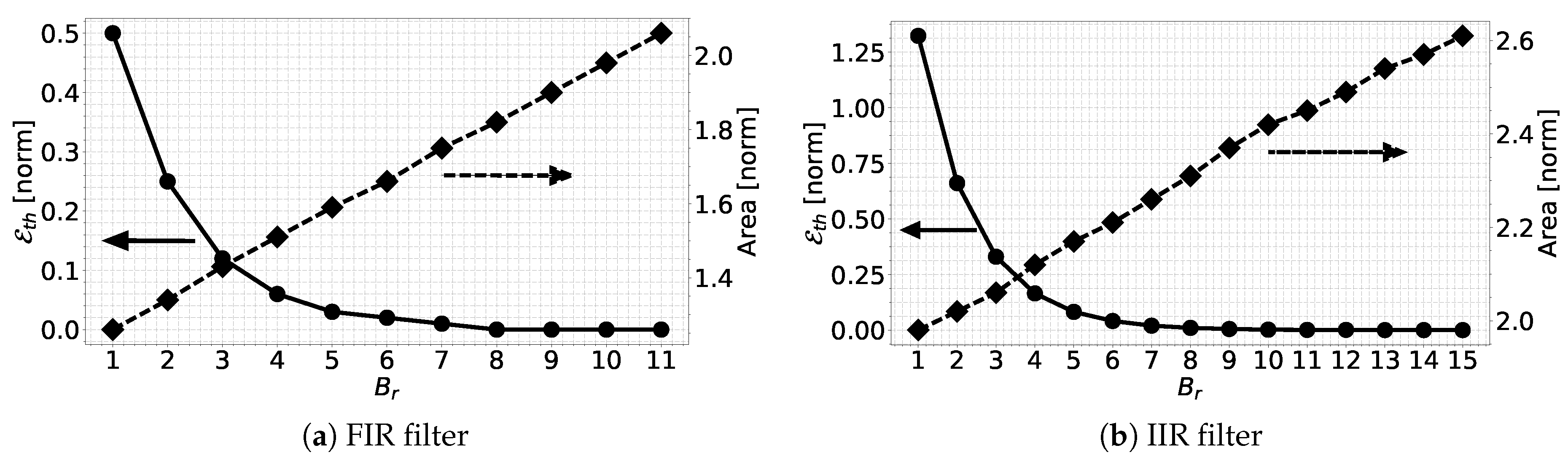
2.2. Design and Area Overhead

The design of the replica circuit and that of the control circuitry introduces some overhead, which should be carefully weighted against the actual savings brought by AVOS. The main challenge is to limit the area and delay penalty while guaranteeing the desired output quality. As a preliminary analysis, we report the design characterization for the two considered benchmarks. We implemented an entire set of RPR-ANT circuits by changing the precision of the replica circuit, namely reducing the input bit-width from 1 to $B-1$, where B is the bit-width of the original circuit. For each implementation, we computed the error threshold (${\mathcal{E}}_{th}$) of the decider unit over the experimental test bench input patterns (Section 4.1) by applying the formula explained in [23]:

$${\mathcal{E}}_{th}=\underset{inputpatterns}{max}\mid y_o\left[n\right]-y_r\left[n\right]\mid$$

(1)

with $y_o$ the error-free output and $y_r$ the output of the replica circuit. Fixing ${\mathcal{E}}_{th}$ in such a way ensures that the output of the circuit Y is equal to the main circuit output $Y_m$ in absence of timing errors.

Figure 2 shows the trend of ${\mathcal{E}}_{th}$ normalized over the output range of $y_o$ ($y_{range}=\mid max\left(y_o\right)-min\left(y_o\right)\mid$) and the area overhead of the architecture versus the number of the replica bits ($B_r$). As expected, the decision threshold increased exponentially when $B_r$ dropped, as shown in [23]. The area overhead, with respect to baseline circuit, increased almost linearly. For the FIR filter, the area ranged from 1.26× to 2.06× for $B_r$ equal to 1 and 11, respectively. In the IIR filter case, even with $B_r$ = 1, the area was 1.98× larger than the baseline filter, and peaked up to 2.61× for $B_r$ = 15. Such large area overhead was due to the internal characteristics of the filters, i.e, the feedback branches of IIR in direct form I.

Hereafter, for the sake of readability, the RPR-ANT strategy is simply labeled as ANT.

3. Approximate Error Detection-Correction (AED-C) via Tunable Error-Detection (TunED)

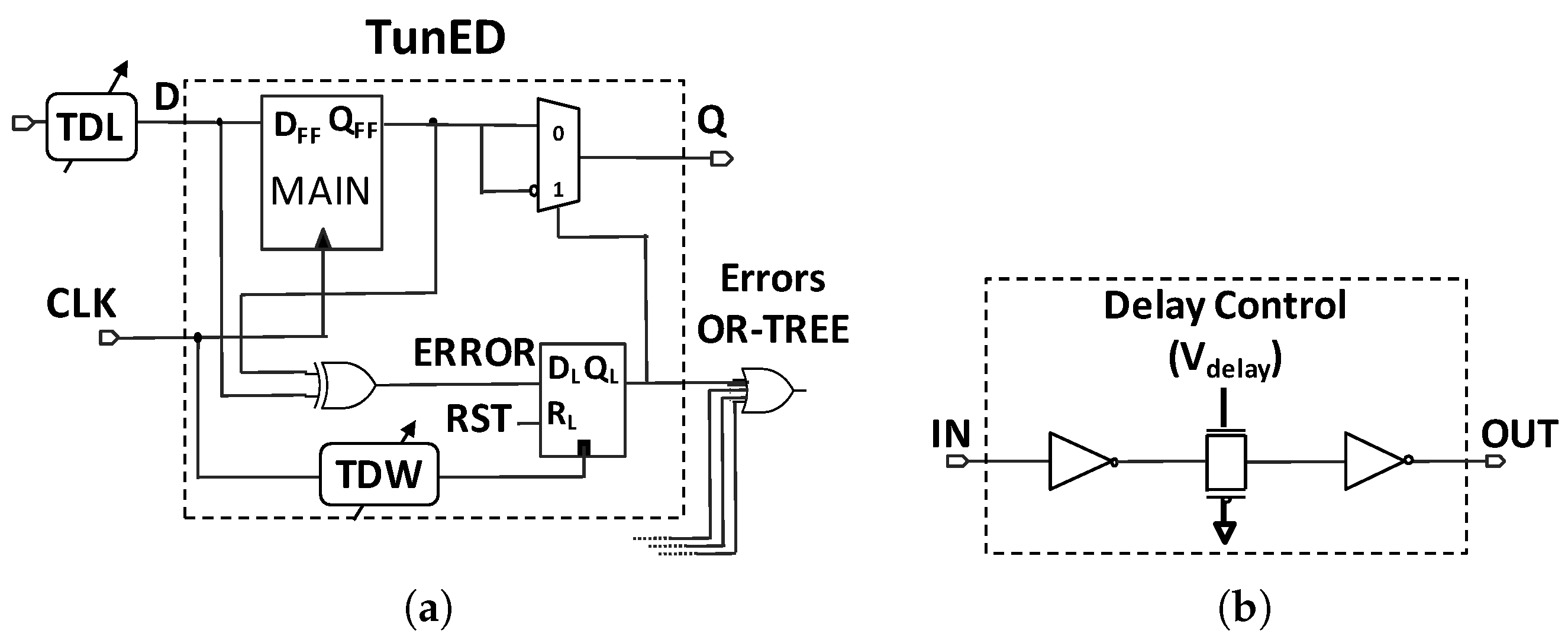
3.1. Implementation

Since AED-C is a generalization of the Razor approach, a proper understanding passes through the description of the Razor mechanism. The following subsections review all the circuit-level implementation details.

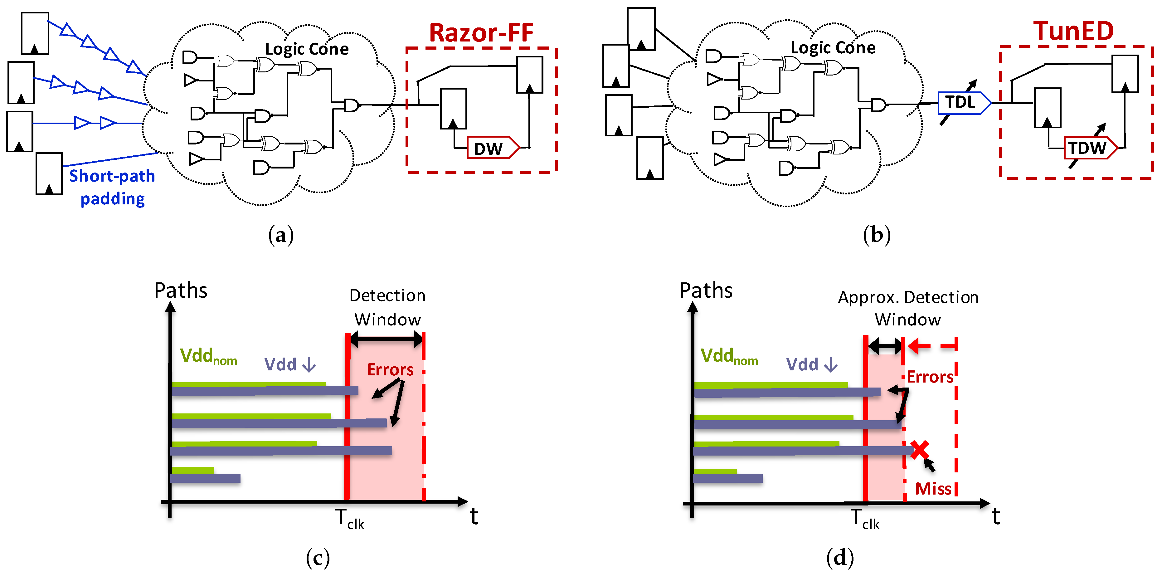
3.1.1. From Razor to AED-C

Razor implements the error detection through special Flip-Flops (FFs), the Razor-FFs in fact (Figure 3a), which sample the combinational output of a logic-cone at two different instants of time: firstly at the rise edge of the clock through the main FF, and secondly after a predefined timing window, the Detection Window (DW), by means of shadow FF. A parity check on the two time-skewed samples returns an error flag: a match implies a correct logic computation, and hence, the availability of some timing slack that can be consumed through $Vdd$ scaling eventually; a mismatch implies the input of the main FF changed after the set-up time, and hence a timing violation. The timing error is recovered using a correction mechanism, e.g., pipe-stalling and refreshing [16] or instruction replay [19]) for micro-instructed architectures, or error logic masking [18] for generic random logic. Both error detection and correction are performed locally, i.e., on each single Razor-FF.

The supply voltage is regulated using the Error Rate ($ER$), that is the number of timing faults detected during a monitoring period. The latter is an integer multiple of the clock-period, while the number of timing faults is the number of clock-cycles during which at least one Razor-FF detected a timing violation. It is worth noting that the error flags generated by each Razor-FFs are all OR-ed, thus generating a global error signal that represents the timing compliance of the whole circuit. If $ER$ is smaller than a user-defined threshold $E{R}_{th}$, then the $Vdd$ can be lowered, otherwise $Vdd$ is raised. Different control policies can be implemented that alter the voltage-scaling and $E{R}_{th}$ is the key parameter to play with: the larger is the $E{R}_{th}$, the faster is the $Vdd$ scaling. However, since error correction is a costly procedure, an energy–performance tradeoff exists. A fast voltage lowering may induce latency and power penalties due to the larger number of corrections [16,19], while a slow voltage lowering is more conservative but it reduces the energy savings. Since there is no general rule, $E{R}_{th}$ is empirically chosen depending on the design specs.

Razor has been conceived to cover the occurrence of all the timing faults (Always-correct scaling). This explains why the DW is taken as large as possible (Figure 3c), usually 50% of the clock period [16]. It is worth noting that DW is statically defined at design-time and that its implementation hides critical issues that are detailed in the next subsection. The AED-C elaborates on Razor and introduces the concept of Tunable Error-Detection (TunED) [25]. TunED leverages Razor-FF enhanced with a Tunable Detection Window (TDW), that is a tunable clock skew between main FF and the shadow FF (Figure 3b). TunED can be understood as an elastic Razor-FF. The TDW alters the resolution of the error detection and hence the faults covered by the timing sensors. As graphically depicted in Figure 3d, the smaller is the TDW, the larger is the number of uncovered latent faults (hence, Approximate Error Detection). The probability of miss-detected faults gets larger as the TDW reduces. This is the enabling mechanism for AED-C. In fact, the TDW is the knob that regulates the level of approximation in detecting errors, i.e., in computing the error rate value $ER$. A small TDW implies more miss-detection (lower $ER$) and thus a faster $Vdd$ scaling, which leads the circuit to low energy and low quality, whereas large TDW guarantees high quality but less energy savings as more faults are properly detected and corrected (higher $ER$). When TDW is set as 50% of the clock-period, AED-C approaches the Razor behavior.

As with Razor, the voltage scaling is operated using the error rate as main feedback to the power management unit. The error flags generated by the timing sensors are OR-ed and the resulting events are counted over the monitor period. Given $E{R}_{th}$ as the error threshold, an error rate smaller than $E{R}_{th}$ drives a $Vdd$ reduction, otherwise the $Vdd$ is increased to save the cost of error corrections. In this case, the error rate can be tuned playing with the width of the TDW. Unlike ${\mathcal{E}}_{th}$, the error threshold in ANT, which refers to the magnitude of the output error, $E{R}_{th}$ has a weak correlation with the arithmetic meaning of the output error. In fact, $E{R}_{th}$ is a measure of the rate of error flags raised by timing sensors, which all have the same weights (or “importance”); namely, in AED-C, the quality degradation is bounded by the paths activity. This represents an important distinction when compared to the ANT strategy.

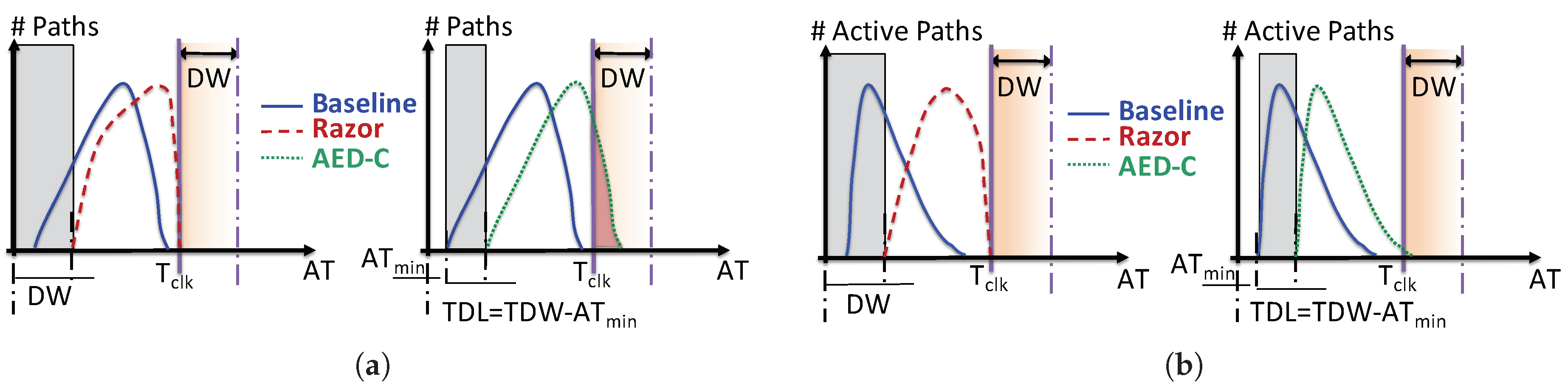
3.1.2. Understanding the Short-Path Race and the Dynamic Short-Path Padding

Razor suffers from the so-called short-path race, which manifests when a short-path and a long-path connected to the same end-point get sequentially activated at clock-cycle $t_i$ and $t_{i-1}$, respectively. Under such condition, the skewing mechanism implemented within the timing sensors fails. Razor-FFs, as well as TunED, would not be able to make distinction between the activation of the short-path within the DW and the activation of the long-path beyond the clock edge. As a result, “false” error detection may occur.

A common practice to address the short-path race is to apply a short-path padding using a standard hold-fixing procedure. The latter consists of delaying all the short-paths in a way that their arrival time becomes larger than $DW$. The delay is implemented by means of optimally placed dummy buffers (overview in Figure 3a). The resulting effect is qualitatively shown with the left plot of Figure 4a, where the solid line is the static path distribution of the original circuit while the dotted line is the same static distribution after the short-path padding. Unfortunately, the short-path padding is a static method, which contrasts with the dynamic nature of the tunable detection strategy. The work described in [28] suggests dynamic short-path padding as an effective patch. A Tunable Delay Line (TDL) is inserted at end-points of the circuit (overview in Figure 3b), where timing sensors are placed, and then the TDL is adjusted at run-time following the modulation of the detection window. More in detail, the TDL is tuned such that the arrival time of the shortest path ($A{T}_{min}$) is delayed beyond the DW. The rule is given as follows:

$$TDL=TDW-A{T}_{min}$$

(2)

The effect is qualitatively shown with the right plot of Figure 4a, where the solid line is the static path distribution of the original circuit while the dotted line is after the TDL insertion.

An important observation is that the TDL affect all the timing paths, even the longest ones, which may suffer early sampling (filled red region in the picture). At a first glance, this issue might be seen as a potential impediment. However, a more accurate analysis reveals the problem practically fades. The longest paths have a lower activation probability [29] and their latent faults are rarely excited, which is the same concept of timing speculation. This is graphically depicted in the right plot of Figure 4b, which shows only a very marginal subset of frequent paths enter the detection window with negligible effect on the error-rate. Needless to say, much depends on the actual workload. The experiments collected in [24,25] prove this strategy is much more efficient than static short-path. Although a detailed discussion is out of the scope of this work, a brief qualitative discussion motivates those findings. Apart from area overhead due to buffers insertion [28,30], short-path padding also affects the supply-voltage scaling. A compression of the timing paths towards the clock edge ($T_{clk}$) implies a redistribution of the internal switching activities, that is, the most active get close to the clock-edge, as shown in the left plot of Figure 4b. This issue, also known as “wall-of-slack”, represents a serious impediment: even small reduction of the $Vdd$ produce a huge number of timing faults as the entire “wall” moves into the detection window of the timing sensors. By contrast, dynamic short-path padding does not suffer from this issue as the dynamic path distribution grows smoother.

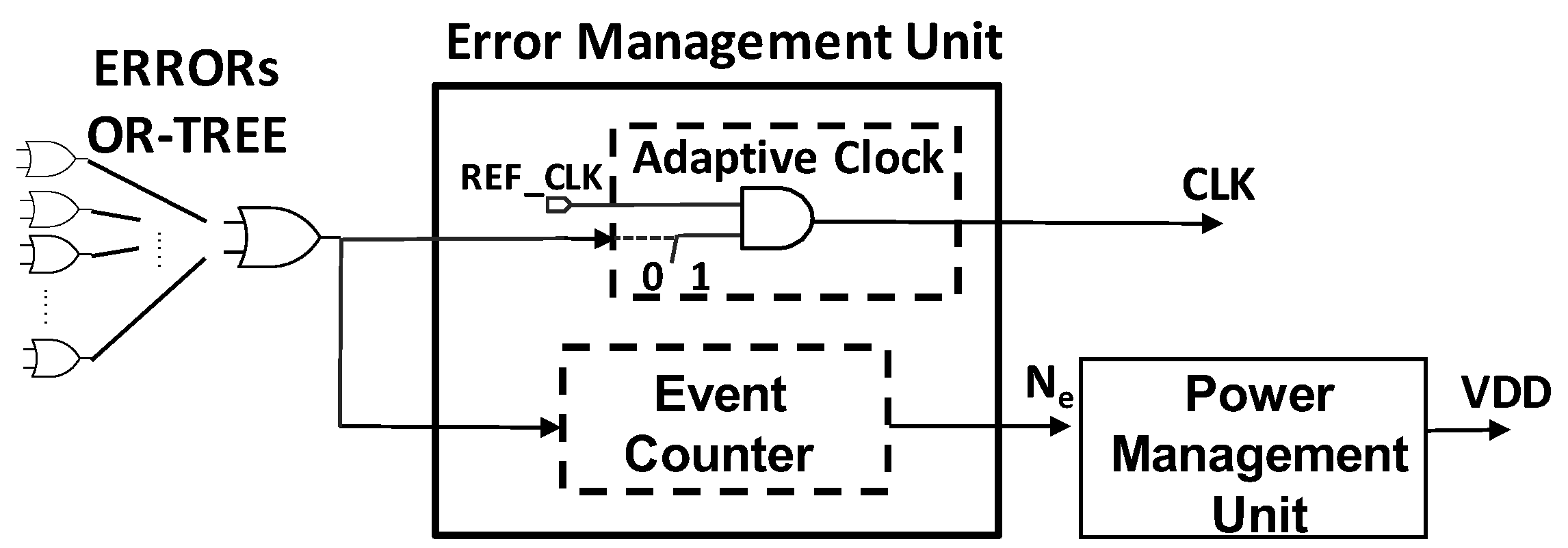
3.1.3. Circuit-Level Details

Figure 5a shows the circuit implementation of the TunED timing sensor deployed in the AED-C scheme [25]. It consists of a Razor-FF [16] augmented with: $\left(i\right)$ the TDW; and $\left(ii\right)$ the logic masking circuitry for error correction. The TDW is implemented as shown in Figure 5b: a pair of inverters interleaved with a transmission gate whose ON-resistance is voltage-controlled using the external signal V${}_{delay}$; a larger V${}_{delay}$ reduces the equivalent load ensuring a smaller delay and hence a smaller detection window. A set-up time violation occurs when the input of the main flip-flop switches within the detection window. The error flag is produced through the XOR gate placed between pins D${}_{FF}$ and Q${}_{FF}$ and then sampled in the shadow latch. Once detected, the error is locally corrected through logic masking: the MUX switches the main output Q with the 1’s complement of the value stored in the main FF.

Although locally computed, the error correction requires a more complex clock-gating mechanism to guarantee a proper propagation of the new corrected output. This is managed through a dedicated unit called Error Management Unit (EMU) (Figure 6). The latter implements an error-driven clock-gating where the clock-enable is generated by OR-ing the flag of all the timing-monitors in the circuit. As soon as one timing sensor detects a timing fault, the circuit is halted for one clock-cycle to allow the right propagation of the corrected value (obtained through the logic masking described above). The EMU also collects the error statistics, i.e., the number of error occurrences $N_e$ within a pre-defined monitoring period of N clock cycles (N = 10${}^3$ in this work). The Power Management Unit (PMU) uses $N_e$ as the error rate that drives the voltage scaling.

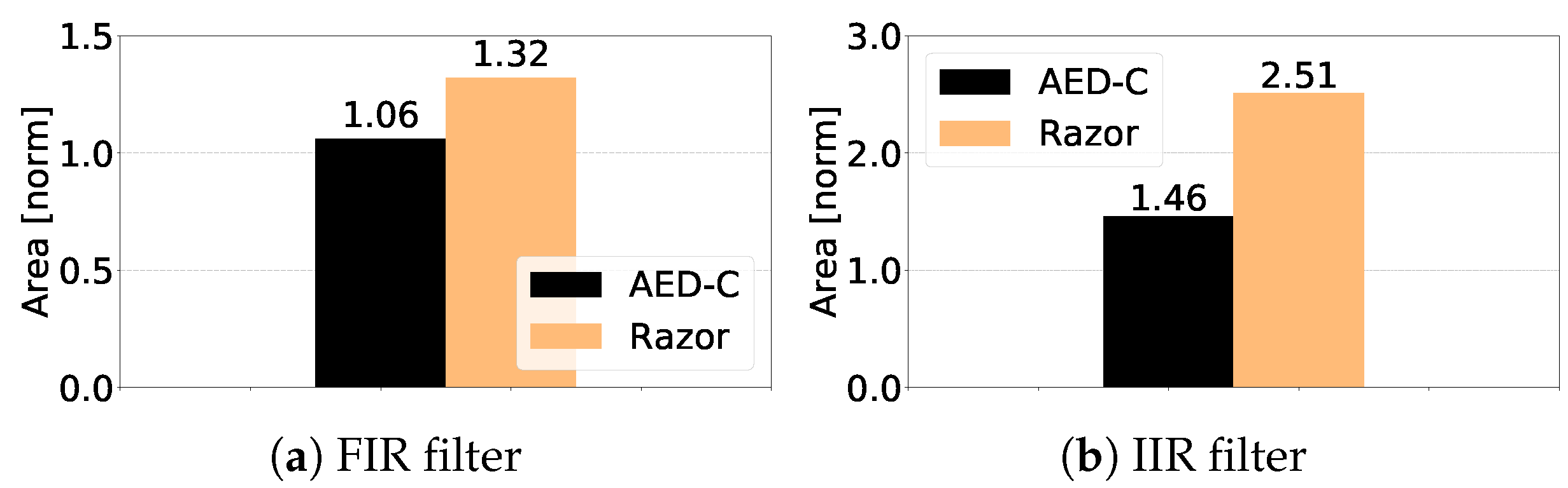
3.2. Area Overhead Characterization

The design flow for both Razor and AED-C encompassed the following steps: (i) timing-driven logic synthesis using 28-nm CMOS industrial technology libraries and critical path end-points identification at the lower bound of the voltage scaling range ($Vdd\in$ [0.60 V,   1.10 V] in this work); and (ii) timing sensors placement, i.e., for each critical end-point, standard FFs were replaced, respectively, with Razor-FF and TunED. These timing sensors were both implemented as reported in Figure 5a except that Razor has a static detection window and does not use TDL but dummy buffers to solve the short-path padding issue.

Despite the use of more complex timing sensors, the AED-C area overhead is lower than that of Razor. Figure 7 shows a comparison between the two for both FIR and IIR filters. For FIR, the area overhead by AED-C was 1.06× against 1.32× of Razor; the gap was even larger for IIR, 1.46× vs. 2.51×. These results are a direct consequence of the short-path padding procedure. The TunED approach solves the races using only few TDLs on the critical endpoints, while Razor static padding operates on a huge number of short-paths. The IIR clearly shows the extent of this problem, as its design shows a feedback network with many short-paths to be “padded”.

4. Experimental Setup

4.1. Benchmarking

Adaptive energy–accuracy scaling strategies work well on those applications that show a certain degree of tolerance to errors. More specifically, on those applications where output errors do not affect, or weakly affect, the quality of results perceived by the end-users (usually humans). Most of such applications make extensive use of DSP algorithms/circuits whose computational kernels are built upon a Multiply-and-Accumulate (MAC). We can mention Discrete Cosine Transform (DCT), Fast Fourier Transform (FFT), CORDIC and Digital Filters. In this work, we focused on spectral audio signal filtering, i.e., FIR and IIR: (i) they are intrinsically error-resilient and commonly adopted in error-resilient applications; and (ii) they make extensive use of MAC operations. As an additional piece of information, one should consider that the architectures of FIR and IIR substantially differ. The IIR circuit has backward connections, which impact the way errors propagate, while the FIR is a feed-forward architecture. Hence, they can be considered as two representative samples.

The proposed work offers a parametric characterization of the compared techniques over a set of modified open source benchmarks. As anticipated above, the benchmarks were two digital filters designed, optimized and mapped using a 28-nm FDSOI CMOS design-kit by a customized design flow integrated into a commercial design platform (Synopsys Galaxy: Design Compiler, IC compiler, Version O-2018.06-SP4) through dedicated TCL scripts. The design flow ran the classical design stages, from timing-driven, low-power logic synthesis up to signal routing; AED-C required an additional stage that encompassed the TunED-monitors/TDLs insertion at the critical end-points, as described in the design flow details of Rizzo et al. [24].

The benchmarks were simulated using non-uniform input distributions and realistic input patterns. The simulations aimed at emulating real-life applications where data maintain a certain spatial/temporal correlation, which is the actual condition under which adaptive strategies gain most of their advantage. For this reason, the sequence of three different baseband audio signals ($5\times {10}^6$ samples in total) was used as test bench. They covered different context scenarios, i.e., different input-data distributions:

• $Audio$-1: Noiseless voice recording; the switching activity of the LSBs is very low for a long portion of the stream.
• $Audio$-2: Taken from an office conversation recording; samples present low noise and inputs have homogeneous switching activity.
• $Audio$-3: Outdoor conversation; the recording is noisy and the switching activity of the inputs quite irregular, due to abrupt changes of input workload.

These three different input distributions are very likely to activate a large spectrum of paths, from shorter to longer ones. Interested readers can refer to the work in [25], where a detailed analysis shows how these different input distributions produce significantly different Energy–Accuracy tradeoff.

4.2. Voltage Over-Scaling Simulation Framework

An in-house tool that simulates voltage over-scaling was integrated into Mentor QuestaSim. It runs a functional simulation with back-annotated SDF delay information extracted through a commercial Static Timing Analysis engine, Synopsys PrimeTime, loaded with technology libraries characterized at different supply voltages; for those supply voltages not available in the library set, we used derating factors embedded into PrimeTime. The supply voltage ranged from 0.60 V to 1.10 V with steps of 20 mV. It is worth noting that voltage scaling was simulated in different ways for AED-C and ANT. In the first case, the voltage scaling followed the input workload, thus $Vdd$ changed dynamically during the test bench simulation. In the second, the voltage was changed statically, i.e., the entire test bench ran for each and every voltage in the range [0.60 V,   1.10 V].

The power dissipation was estimated using a probabilistic power models (Synopsys PrimePower) with back-annotated signal statistics extracted from functional simulations using saif format files. The energy consumption was estimated considering the supply voltage profiles collected from voltage over-scaling emulations. The power of the delay lines was measured through PrimePower, using pass transistor cells characterized through HSPICE simulation.

4.3. Figures of Merit

The comparison between AED-C and ANT included the following metrics:

• $Vd{d}_{avg}$: The average $Vdd$ obtained during test bench voltage over-scaling simulation for AED-C based timing speculation. For RPR-ANT, the average voltage corresponded to the $Vdd$ employed during the test bench simulation.
• Energy per Operation (EPO): The ratio of energy consumed to the number of operations completed.
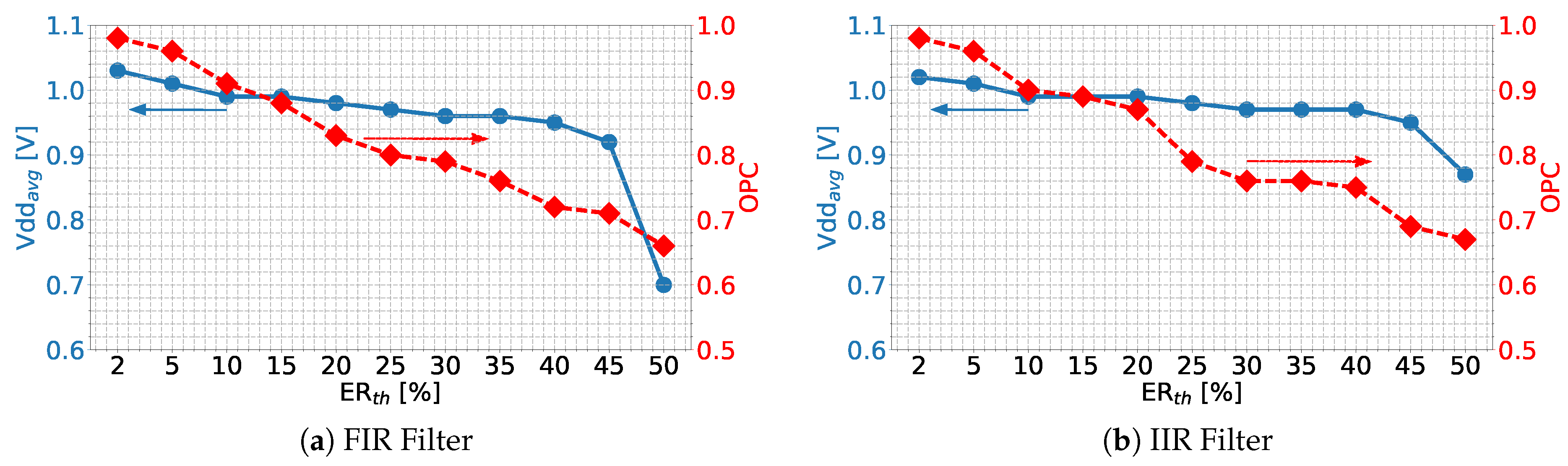
• Operation per Clock Cycle (OPC): The ratio of the number of executed operations to the total number of clock cycles, considering that in AED-C techniques error corrections through logic masking need a cycle of clock gating. For RPR-ANT, the OPC was always 1, since no performance loss was conceived.
• Normalized Root Mean Squared Error (NRMSE):

  $$NRMSE=\sqrt{\frac{{\sum }_{i=0}^n{(y\left[i\right]-y_o\left[i\right])}^2}{n}}·\frac{1}{\mid max\left(y_o\right)-min\left(y_o\right)\mid }$$

  (3)

  with y the value sampled at the output of the circuit, $y_o$ the right output value, and n the total number of operations. The absolute values of the the maximum and minimum of $y_o$ difference defined the output dynamic range. $NRMSE$ quantified the quality of results.
• Maximum Absolute Error (MAE): expressed in ${log}_2$ form,

  $$MAE={log}_2⌊\underset{inputpatterns}{max}\mid y\left[i\right]-y_o\left[i\right]\mid ⌋-1$$

  (4)

  with y the value sampled at the output of the circuit and $y_o$ the right output value. This metric representation collapses the maximum error on a single bit of the output.

5. Experimental Results

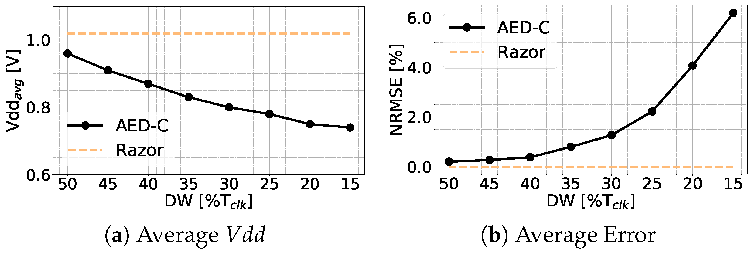
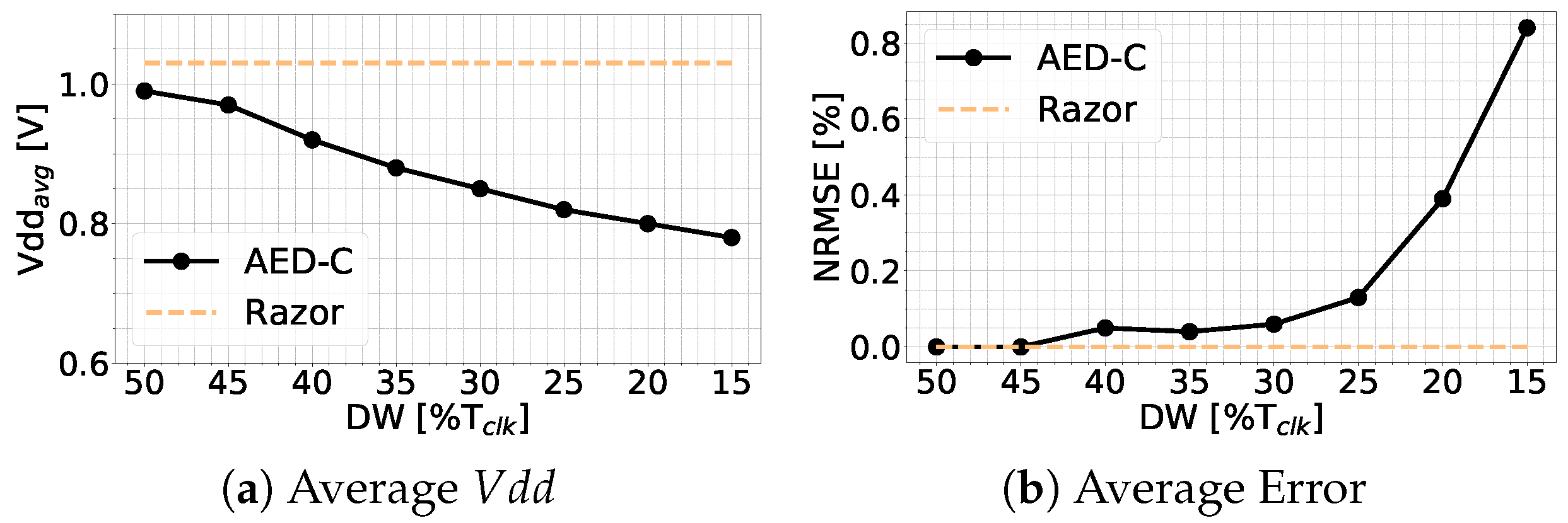
5.1. Razor vs. AED-C

Although the objective of this work was the comparison of approximate methods, i.e., ANT and AED-C, a preliminary analysis between a classical Razor and AED-C was paramount.

Razor was implemented using the following configuration to limit the performance loss due to errors correction:

• Detection Window:$DW=50\%·T_{clk}$;
• Monitoring period:N = 10${}^3$ clock cycles; and
• Error Rate Threshold:$E{R}_{th}$ = 2%.

The AED-C was set with the same values, except for the detection window, which was used as a parameter: $TDW\in [15\%·T_{clk},50\%·T_{clk}]$, regular intervals of $5\%·T_{clk}$.

Figure 8a and Figure 9a show the results of voltage scaling efficiency collected for FIR and IIR, respectively. While Razor has a fixed $DW$ width, thus a single $Vd{d}_{avg}$ value highlighted with a dashed line, AED-C enables different Energy–Quality operating points by tuning the $DW$ width. As expected, by reducing the $DW$, a more aggressive $Vdd$ scaling could be obtained. In fact, $Vd{d}_{avg}$ decreased quickly as the $DW$ width became smaller for both FIR and IIR filters. In Razor, the insertion of buffers for short-path padding compressed the active paths toward the clock ed,ge inducing an increase of the error rate. That made the voltage scaling slower: $Vd{d}_{avg}$ did not go below 1.03 V ( 1.02 V) for FIR (IIR). With AED-C, the path distribution kept the same shape (only right shifted), ensuring a smoother increase of the error rate. This was an additional key advantage of the AED-C strategy. The reduction of the error-coverage, namely the reduction of $TDW$, implied a proportional reduction of the TDL. As the TDL became smaller, the path distribution shifted back to its original shape, leaving the most active paths behind the detection window. When considering the FIR benchmark, the $Vd{d}_{avg}$ reduction was substantial: from 0.99 V at $DW$ = $50\%·T_{clk}$, to 0.78 V at $DW$ = $15\%·T_{clk}$; for the IIR filter case, the $Vd{d}_{avg}$ reduction was in the range [0.96 V, 0.74 V].

Concerning the quality of the output, while Razor showed zero degradation for both filters, for AED-C, the quality of the output reduced as the as the detection mechanism became more approximated. This trend is clearly reported in Figure 8b and Figure 9b. The $NRMSE$ increased from 0% at $DW$ = $50\%·T_{clk}$ to 0.84% for $DW$ = $15\%·T_{clk}$, while, for the IIR filter, the $NRMSE$ rose from 0.2% at $DW$ = $50\%·T_{clk}$ to 6.19% at $DW$ = $15\%·T_{clk}$. It is worth emphasizing the error showed bigger magnitude since miss-detected timing error was trapped in the filter feedback network, propagating back to the internal paths and persisting until a sequence of input patterns masked it. It is worth noting that the IIR filter implemented with AED-C presented an average error greater than zero when $DW$ = $50\%·T_{clk}$; this result was a direct consequence of the smoother shape of the dynamic path distribution induced by AED-C, as explained in Section 3.1.2. In fact, even with the maximum value of the $DW$, the $Vdd$ scaled more aggressively than Razor (on average 0.96 V against 1.02 V) leading to error miss-detection, thus output quality degradation.

The throughput of both Razor and AED-C showed a strict relation with $E{R}_{th}$, as demonstrated in [28]. Since $E{R}_{th}$ was the same (2%), the worst-case $OPC$ was 0.98 (2% throughput degradation).

These results confirm that moving from Razor to AED-C enabled an efficient energy–accuracy tradeoff. One may argue that an approximate version of Razor could have been obtained using the error-threshold $E{R}_{th}$ as a control knob instead of tuning the detection window $DW$. However, energy savings would have been much lower due to large performance penalties. The use of a larger $E{R}_{th}$ implies the raise of timing errors to correct. More timing errors means that the number of cycles wasted for correction increases, hence the $OPC$ decrease quickly with $E{R}_{th}$. To give a proof, the plots in Figure 10 show $Vd{d}_{avg}$ and $OPC$ as function of the error threshold $E{R}_{th}$ for both FIR and IIR; $E{R}_{th}$ was in the range $[2\%,50\%]$. The workload is the one described in Section 4.1. While $E{R}_{th}$ increased, the $Vd{d}_{avg}$ reduced as expected: from 1.03 V to 0.70 V for FIR and from 1.02 V to 0.87 V for IIR. However, the performance loss was substantial as the $OPC$ decreased: from 0.98 to 0.66 (almost two clock cycles for each operation) for FIR and from 0.98 to 0.67 for IIR. With AED-C, the $OPC$ overhead was 2% at worst.

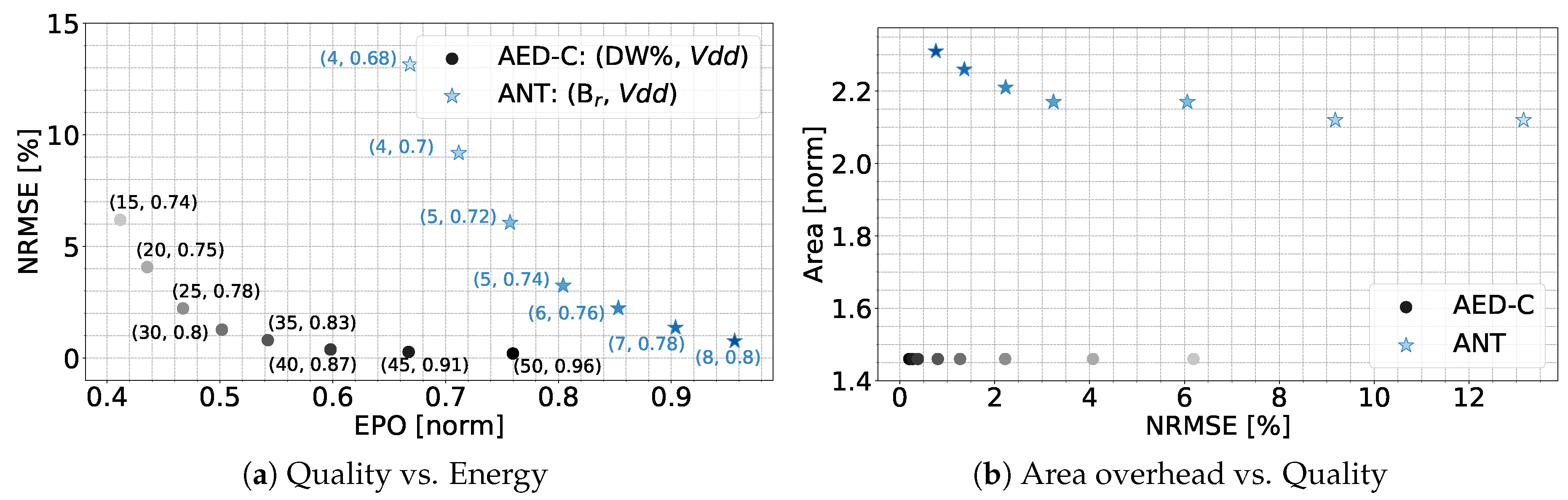
5.2. ANT Vs. AED-C

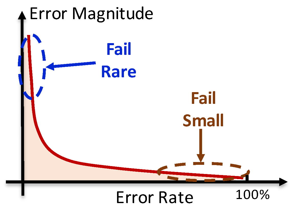
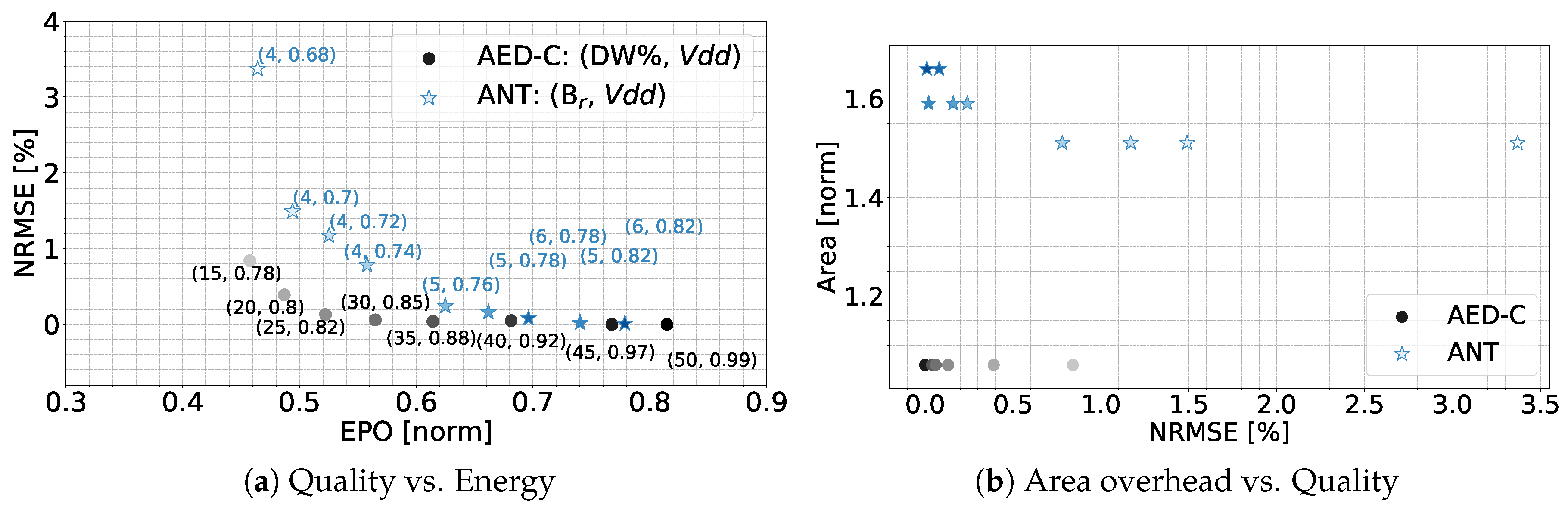
5.2.1. Qualitative Analysis

Under the output quality point of view, ANT and AED-C can be associated with two distinct classes of approximate techniques using the formal definition given in [31,32] and reported in Figure 11. ANT belongs to the class of fail small applications. The errors introduced by the voltage scaling remain “small” in magnitude (as they are bounded by the precision of the replica circuit) but quite frequent. AED-C belongs the class of fail rare. The error magnitude is usually quite large (the long timing paths of arithmetic circuits are commonly on the MSB of the output) but infrequent (long timing paths are activated rarely). This separation reflects the difference between voltage scaling using approximate computing and voltage scaling using approximate error detection. The quantitative analysis presented in the next section confirmed this trend through a more concrete comparison.

5.2.2. Quantitative Analysis

To perform a formal comparison between ANT and AED-C, figures of merit such as quality of results, energy savings, performance and area overhead were assessed. Since there are too many possible design variables and settings to show, this section provides a more compact, yet complete Pareto analysis.

Let us first analyze the FIR filter. Figure 12a shows the Pareto points in the quality vs. energy space ($NRMSE$ vs. $EPO$). The AED-C points (black dot) are labeled with the caption (DW%, $Vd{d}_{avg}$) and the ANT points (blue stars) are labeled with (B${}_r$, $Vdd$), with $B_r$ as the number of bits of the replica circuit and $Vdd$ is the operating voltage. It is worth noting that, in the ANT case, the valid Pareto points are only those whose operating voltage ensures no timing violations in the replica circuit.

As a general trend, AED-C showed a better energy–quality tradeoff, except for the rightmost points at $DW$ = 50% of $T_{clk}$, which was dominated by the ANT point (6, 0.82). The results can be simply explained considering that the ANT architecture required a more approximated replica circuit, i.e., lower $B_r$, to achieve the same energy savings of AED-C; however, a too approximated replica induced a quick increase of error.

To better appreciate this trend,

Table 1. Quantitative comparison summary: FIR filter.

Technique	Vdd	EPO	OPC	N. Errors	NRMSE	MAE	Area
	[V]	[norm]			[%]	[norm]	[norm]
	Min. EPO point
AED-C (DW = 15%)	0.78	0.46	0.98	3226	0.84	21	1.06
ANT (B${}_r$ = 4)	0.68	0.46	1.00	1,382,023	3.37	17	1.51
	NRMSE-EPO Knee point
AED-C (DW = 25%)	0.82	0.52	0.98	114	0.13	20	1.06
ANT (B${}_r$ = 5)	0.78	0.66	1.00	97,664	0.16	16	1.59
	Min. NRMSE point
AED-C (DW = 50%)	0.99	0.81	0.98	16	0.01	17	1.06
ANT (B${}_r$ = 6)	0.82	0.78	1.00	11,746	0.01	16	1.66

gives a more detailed view. In the first row (Min. EPO point), it shows the comparison between the points of ANT and AED-C with the highest energy-efficiency: AED-C${}_{(15,0.78)}$ and ANT${}_{(4,0.68)}$. For almost the same energy, AED-C gave results of a much higher quality ($NRMSE$ = 0.84% for AED-C vs. 3.37% for ANT). Evidence of the AED-C superiority is also given by looking at the second row (NRMSE-EPO Knee point), which collects the metrics for ANT and AED-C across the knee of their $NRMSE-EPO$ Pareto curves: AED-C${}_{(25,0.82)}$ and ANT${}_{(5,0.78)}$. For almost the same quality of results, AED-C outperformed ANT in terms of energy savings ($EPO$ = 0.52 for AED-C vs. 0.66 for ANT). Even though the ANT implementation reached a lower $Vdd$, its energy savings was limited by the architectural overhead. This aspect emerged clearly from the Area–Quality Pareto analysis of Figure 12b. For the sake of clarity, it should be noticed that at best accuracy Pareto points, as reported in Table 1 third row (Min. NRMSE point), ANT presented slightly lower EPO than AED-C, i.e., 0.78 vs. 0.81. When accuracy is the priority, the $DW$ should be taken larger. For such conservative case, ANT was more efficient than AED-C, in which the activation of the longest paths limited the voltage scaling (hence, the energy savings).

To ensure a specific output quality, the replica circuits need more arithmetic precision and they take huge silicon area. For minimum output degradation, the area overhead reached with ANT was more than 60%, too much for real-life circuits. It is worth noting that AED-C showed a constant area overhead as the different configurations were obtained only by tuning the $TDW/TDL$ width, with no micro-architectural modifications. Not just area, also throughput ($OPC$) needs special care. Table 1 shows that ANT did not suffer any performance penalty, while AED-C was 2% slower due to error detection-corrections. It is worth highlighting how the distribution of the timing errors for both techniques followed the classification made at the beginning of this section. As reported in Table 1, AED-C was characterized by a lower number of errors (col. N. Errors, over $5\times {10}^6$ input patterns) of high magnitude (col. MAE); the opposite held for ANT, namely more errors of lower amplitude. Although the magnitude of the errors in AED-C is higher than ANT, the effect on the overall quality of results remain acceptable (col. NRMSE).

The comparative analysis performed on the IIR filter emphasized even more what the FIR analysis showed. As reported in Figure 13a and

Table 2. Quantitative comparison summary: IIR filter.

Technique	Vdd	EPO	OPC	N. Errors	NRMSE	MAE	Area
	[V]	[norm]			[%]	[norm]	[norm]
	Min. EPO point
AED-C (DW = 15%)	0.74	0.41	0.98	93387	6.19	30	1.46
ANT (B${}_r$ = 4)	0.68	0.67	1.00	4586948	13.15	26	2.12
	NRMSE-EPO Knee point
AED-C (DW = 35%)	0.83	0.54	0.98	11759	0.80	30	1.46
ANT (B${}_r$ = 5)	0.72	0.76	1.00	2316127	6.01	25	2.17
	Min. NRMSE point
AED-C (DW = 50%)	0.96	0.76	0.98	1548	0.20	27	1.46
ANT (B${}_r$ = 8)	0.80	0.96	1.00	99872	0.76	21	2.31

, AED-C guaranteed higher energy efficiency than ANT and all the ANT implementation were dominated by AED-C. A similar consideration done for FIR still held. Although ANT pushed the supply voltage to lower value, it still could not achieve the same energy of AED-C. Shrinking the ANT replica circuit to $B_r$ = 4 (point ANT${}_{(4,0.68)}$), the $EPO$ became close to that reached with AED-C${}_{(45,0.91)}$, yet with an unacceptable output degradation ($NRMSE$ 13.15% vs. 0.27%). Conversely, for the same $NRMSE$, the area overhead became too large for a realistic implementation (Figure 13b).

5.2.3. On the AED-C Expendability

The proposed AED-C is based on the probabilistic assumption that an efficient voltage over-scaling can be achieved if long paths are rarely activated. This is the same consideration under which both Razor and ANT are built. However, for our AED-C, there might be specific sequences of input patterns for which the Vdd is pushed so low that some paths run beyond the detection window, thus leading to potential miss-detected errors and output quality degradation. This is the main difference with respect to Razor and ANT (which are bounded in terms of quality degradation instead). This also reflects the limits of the AED-C technique: a too frequent activation of the longest paths may limit the voltage scaling and hence the energy savings. There is a trade-off between accuracy and savings. When accuracy is the priority, the Detection Window (DW) should be taken larger. For such conservative cases, ANT may outperform AED-C. This is shown in Figure 12a, where the FIR filter with DW = 45%(50%) $·$$T_{clk}$ showed lower energy savings compared to ANT.

The key of AED-C is that it can be implemented with low design overhead. By contrast, ANT requires a replica circuit that introduces severe area (and hence energy) penalty.

6. Conclusions

This paper introduces a quantitative comparison between two Energy–Quality scaling strategies based on Timing Speculation: Algorithmic Noise Tolerance (ANT) and Approximate Error Detection-Correction (AED-C). The first implements a timing speculation through approximate computing principle, while the latter exploits a more sophisticated approach that is based on the approximation of the error detection mechanism.

The target of this study was to provide a quantitative comparison between ANT and AED-C. A parametric characterization conducted over a set of realistic applications quantified several figures of merit, e.g., energy savings, performance and area overhead. The benchmarks consisted of two digital filters, a FIR and a IIR, both synthesized and mapped onto a commercial FD-SOI CMOS technology at 28 nm. The results collected for a sequence of three different classes of baseband audio signals empirically disclose better efficiency of AED-C with respect to ANT, providing an assessment of the resulting energy–quality and area–quality tradeoff.

References

- Benini, L.; Castelli, G.; Macii, A.; Macii, B.; Scarai, R. Battery-driven dynamic power management of portable systems. In Proceedings of the 13th International Symposium on System Synthesis, Madrid, Spain, 20–22 September 2000; pp. 25–30. [Google Scholar]
- Alioto, M. Ultra Low Power Design approaches for IoT. In Proceedings of the 2014 IEEE Hot Chips 26 Symposium (HCS), Cupertino, CA, USA, 10–12 August 2014; pp. 1–57. [Google Scholar]
- Hameed, A.; Khoshkbarforoushha, A.; Ranjan, R.; Jayaraman, P.P.; Kolodziej, J.; Balaji, P.; Zeadally, S.; Malluhi, Q.M.; Tziritas, N.; Vishnu, A.; et al. A survey and taxonomy on energy efficient resource allocation techniques for cloud computing systems. Computing 2016, 98, 751–774. [Google Scholar] [CrossRef]
- Zakarya, M.; Gillam, L. Energy efficient computing, clusters, grids and clouds: A taxonomy and survey. Sustain. Comput. Inform. Syst. 2017, 14, 13–33. [Google Scholar] [CrossRef]
- Herbert, S.; Marculescu, D. Analysis of dynamic voltage/frequency scaling in chip-multiprocessors. In Proceedings of the 2007 IEEE International Symposium on Low Power Electronics and Design (ISLPED’07), Portland, OR, USA, 27–29 August 2007; pp. 38–43. [Google Scholar]
- Choi, K.; Soma, R.; Pedram, M.; Pedram, M.; Pedram, M.; Pedram, M. Dynamic Voltage and Frequency Scaling Based on Workload Decomposition. In Proceedings of the 2004 International Symposium on Low Power Electronics and Design, Newport Beach, CA, USA, 9–11 August 2004; ACM: New York, NY, USA, 2004; pp. 174–179. [Google Scholar] [CrossRef]
- Peluso, V.; Rizzo, R.G.; Calimera, A.; Macii, E.; Alioto, M. Beyond Ideal DVFS Through Ultra-Fine Grain Vdd-Hopping. In Proceedings of the IFIP/IEEE International Conference on Very Large Scale Integration-System on a Chip, Tallinn, Estonia, 26–28 September 2016; Springer: Cham, Switzerland, 2016; pp. 152–172. [Google Scholar]
- Martin, S.M.; Flautner, K.; Mudge, T.; Blaauw, D. Combined dynamic voltage scaling and adaptive body biasing for lower power microprocessors under dynamic workloads. In Proceedings of the 2002 IEEE/ACM International Conference On Computer-Aided Design, San Jose, CA, USA, 10–14 November 2002; pp. 721–725. [Google Scholar]
- Hemantha, S.; Dhawan, A.; Kar, H. Multi-threshold CMOS design for low power digital circuits. In Proceedings of the TENCON 2008 IEEE Region 10 Conference, Hyderabad, India, 19–21 November 2008; pp. 1–5. [Google Scholar]
- Calimera, A.; Pullini, A.; Sathanur, A.V.; Benini, L.; Macii, A.; Macii, E.; Poncino, M. Design of a family of sleep transistor cells for a clustered power-gating flow in 65 nm technology. In Proceedings of the 17th ACM Great Lakes Symposium on VLSI, Lago Maggiore, Italy, 11–13 March 2007; pp. 501–504. [Google Scholar]
- Kahng, A.B.; Kang, S.; Kumar, R.; Sartori, J. Slack redistribution for graceful degradation under voltage overscaling. In Proceedings of the 2010 Asia and South Pacific Design Automation Conference, Taipei, Taiwan, 18–21 January 2010; pp. 825–831. [Google Scholar]
- Ghosh, S.; Bhunia, S.; Roy, K. CRISTA: A new paradigm for low-power, variation-tolerant, and adaptive circuit synthesis using critical path isolation. IEEE Trans. Comput.-Aided Des. Integrated Circuits Syst. 2007, 26, 1947–1956. [Google Scholar] [CrossRef]
- Austin, T.; Bertacco, V.; Blaauw, D.; Mudge, T. Opportunities and Challenges for Better Than Worst-case Design. In Proceedings of the 2005 Asia and South Pacific Design Automation Conference, Shanghai, China, 18–21 January 2005; ACM: New York, NY, USA, 2005; pp. 2–7. [Google Scholar] [CrossRef]
- Bortolotti, D.; Rossi, D.; Bartolini, A.; Benini, L. A variation tolerant architecture for ultra low power multi-processor cluster. In Proceedings of the 2013 23rd International Workshop on Power and Timing Modeling, Optimization and Simulation (PATMOS), Karlsruhe, Germany, 9–11 September 2013; pp. 32–38. [Google Scholar]
- Ernst, D.; Das, S.; Lee, S.; Blaauw, D.; Austin, T.; Mudge, T.; Kim, N.S.; Flautner, K. Razor: Circuit-level correction of timing errors for low-power operation. IEEE Micro 2004, 24, 10–20. [Google Scholar] [CrossRef]
- Ernst, D.; Kim, N.S.; Das, S.; Pant, S.; Rao, R.; Pham, T.; Ziesler, C.; Blaauw, D.; Austin, T.; Flautner, K.; et al. Razor: A low-power pipeline based on circuit-level timing speculation. In Proceedings of the 36th Annual IEEE/ACM International Symposium on Microarchitecture, San Diego, CA, USA, 3–5 December 2003; pp. 7–18. [Google Scholar]
- Das, S.; Roberts, D.; Lee, S.; Pant, S.; Blaauw, D.; Austin, T.; Flautner, K.; Mudge, T. A self-tuning DVS processor using delay-error detection and correction. IEEE J. Solid-State Circuits 2006, 41, 792–804. [Google Scholar] [CrossRef]
- Valadimas, S.; Tsiatouhas, Y.; Arapoyanni, A. Timing error tolerance in nanometer ICs. In Proceedings of the 2010 IEEE 16th International On-Line Testing Symposium, Corfu, Greece, 5–7 July 2010; pp. 283–288. [Google Scholar]
- Das, S.; Tokunaga, C.; Pant, S.; Ma, W.H.; Kalaiselvan, S.; Lai, K.; Bull, D.M.; Blaauw, D.T. RazorII: In situ error detection and correction for PVT and SER tolerance. IEEE J. Solid-State Circuits 2009, 44, 32–48. [Google Scholar] [CrossRef]
- Krause, P.K.; Polian, I. Adaptive voltage over-scaling for resilient applications. In Proceedings of the 2011 Design, Automation Test in Europe, Grenoble, France, 14–18 March 2011; pp. 1–6. [Google Scholar] [CrossRef]
- Alioto, M. Energy-quality scalable adaptive VLSI circuits and systems beyond approximate computing. In Proceedings of the Design, Automation & Test in Europe Conference & Exhibition (DATE), Lausanne, Switzerland, 27–31 March 2017; pp. 127–132. [Google Scholar] [CrossRef]
- Shim, B.; Shanbhag, N.R. Reduced precision redundancy for low-power digital filtering. In Proceedings of the Conference Record of Thirty-Fifth Asilomar Conference on Signals, Systems and Computers (Cat. No. 01CH37256), Pacific Grove, CA, USA, 4–7 November 2001; Volume 1, pp. 148–152. [Google Scholar]
- Shim, B.; Sridhara, S.R.; Shanbhag, N.R. Reliable low-power digital signal processing via reduced precision redundancy. IEEE Trans. Very Large Scale Integr. (VLSI) Syst. 2004, 12, 497–510. [Google Scholar] [CrossRef]
- Rizzo, R.G.; Calimera, A.; Zhou, J. Approximate Error Detection-Correction for efficient Adaptive Voltage Over-Scaling. Integration 2018, 63, 220–231. [Google Scholar] [CrossRef]
- Rizzo, R.G.; Calimera, A. Tunable Error Detection-Correction for Efficient Adaptive Voltage Over-Scaling. In Proceedings of the 2017 IEEE 1st International New Generation of Circuits and Systems Conference (NGCAS), Genoa, Italy, 6–9 September 2017. [Google Scholar]
- Hegde, R.; Shanbhag, N.R. Energy-efficient signal processing via algorithmic noise-tolerance. In Proceedings of the 1999 International Symposium on Low Power Electronics and Design (Cat. No.99TH8477), San Diego, CA, USA, 17 August 1999; pp. 30–35. [Google Scholar]
- Hegde, R.; Shanbhag, N.R. A low-power digital filter IC via soft DSP. In Proceedings of the IEEE 2001 Custom Integrated Circuits Conference (Cat. No.01CH37169), San Diego, CA, USA, 9 May 2001; pp. 309–312. [Google Scholar]
- Rizzo, R.G.; Peluso, V.; Calimera, A.; Zhou, J.; Liu, X. Early Bird Sampling: A Short-Paths Free Error Detection-Correction Strategy for Data-Driven VOS. In Proceedings of the 2017 IFIP/IEEE International Conference on Very Large Scale Integration (VLSI-SoC), Abu Dhabi, UAE, 23–25 October 2017. [Google Scholar]
- Bowman, K.A.; Tschanz, J.W.; Kim, N.S.; Lee, J.C.; Wilkerson, C.B.; Lu, S.L.L.; Karnik, T.; De, V.K. Energy-efficient and metastability-immune resilient circuits for dynamic variation tolerance. IEEE J. Solid-State Circuits 2009, 44, 49–63. [Google Scholar] [CrossRef]
- Kim, S.; Seok, M. Variation-tolerant, ultra-low-voltage microprocessor with a low-overhead, within-a-cycle in-situ timing-error detection and correction technique. IEEE J. Solid-State Circuits 2015, 50, 1478–1490. [Google Scholar] [CrossRef]
- Chippa, V.K.; Chakradhar, S.T.; Roy, K.; Raghunathan, A. Analysis and characterization of inherent application resilience for approximate computing. In Proceedings of the 50th Annual Design Automation Conference, Austin, TX, USA, 29 May–7 June 2013; p. 113. [Google Scholar]
- Nogues, E.; Menard, D.; Pelcat, M. Algorithmic-level approximate computing applied to energy efficient hevc decoding. IEEE Trans. Emerg. Top. Comput. 2016, 7, 5–7. [Google Scholar] [CrossRef]