


BIoU: An Improved Bounding Box Regression for Object Detection


Abstract
1. Introduction
- The research begins with a background study on object detection and bounding box regression losses in Section 2.
- Section 5 provides an overview of the datasets utilized in this research study.
- Simulation experiments and their results are detailed in Section 6.1.
- Section 6.2 provides background on the experimental setup and deep learning architecture chosen for this research.
- The performance of the proposed BIoU loss is evaluated in Section 7.
2. Literature Review
2.1. Object Detection
- Loss functions to find the bounding box coordinates to localize target objects;
- Classification to identify the target object;
- The first task relies on the loss functions, which give the error between the predicted and ground truth bounding box [31].
2.2. Remote Sensing
2.3. Bounding Box Regression Loss
3. Survey on Axis-Aligned Loss Functions
4. Proposed BIoU Loss Function
5. DataSet Preparation
5.1. Common Objects in Context (COCO)
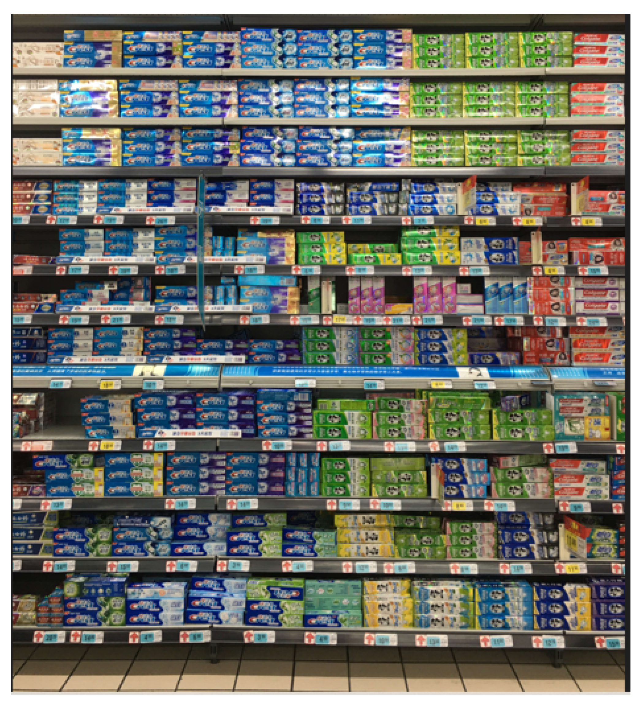
5.2. SKU-110K
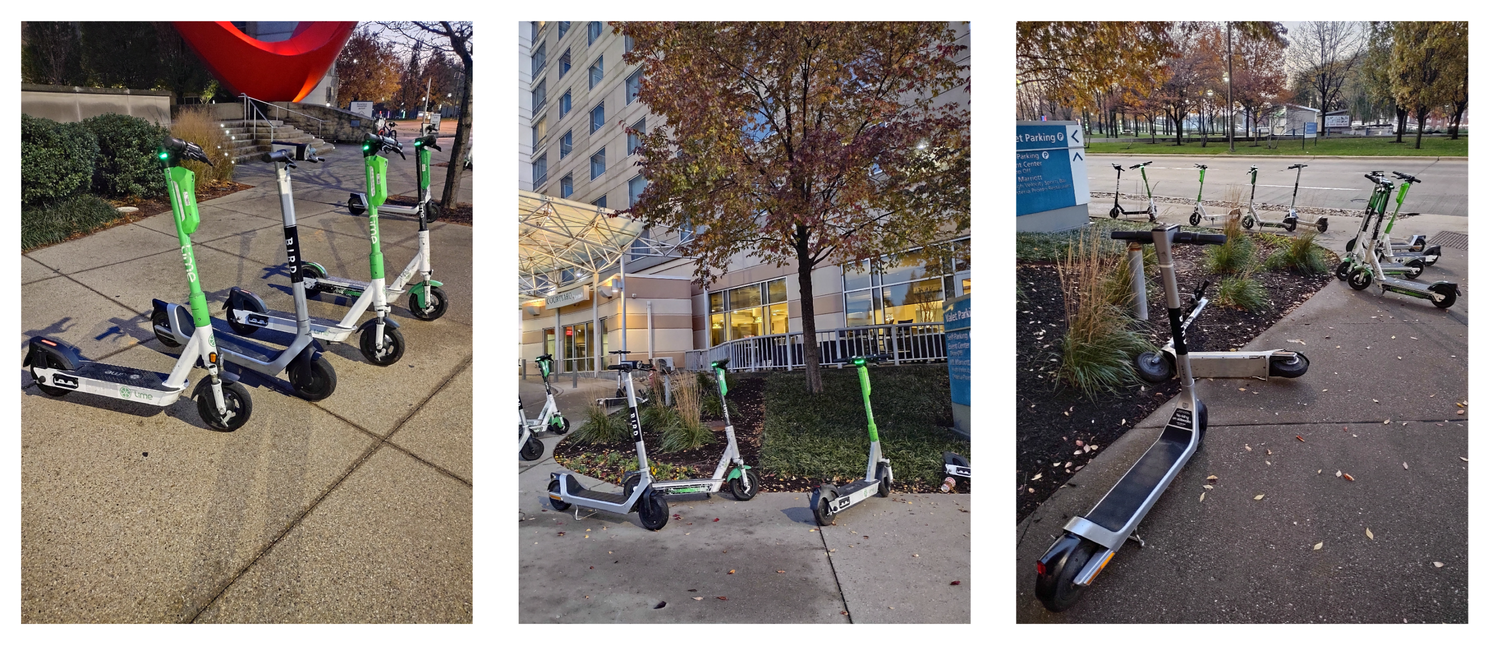
5.3. Custom Dataset
6. Experimental Setup
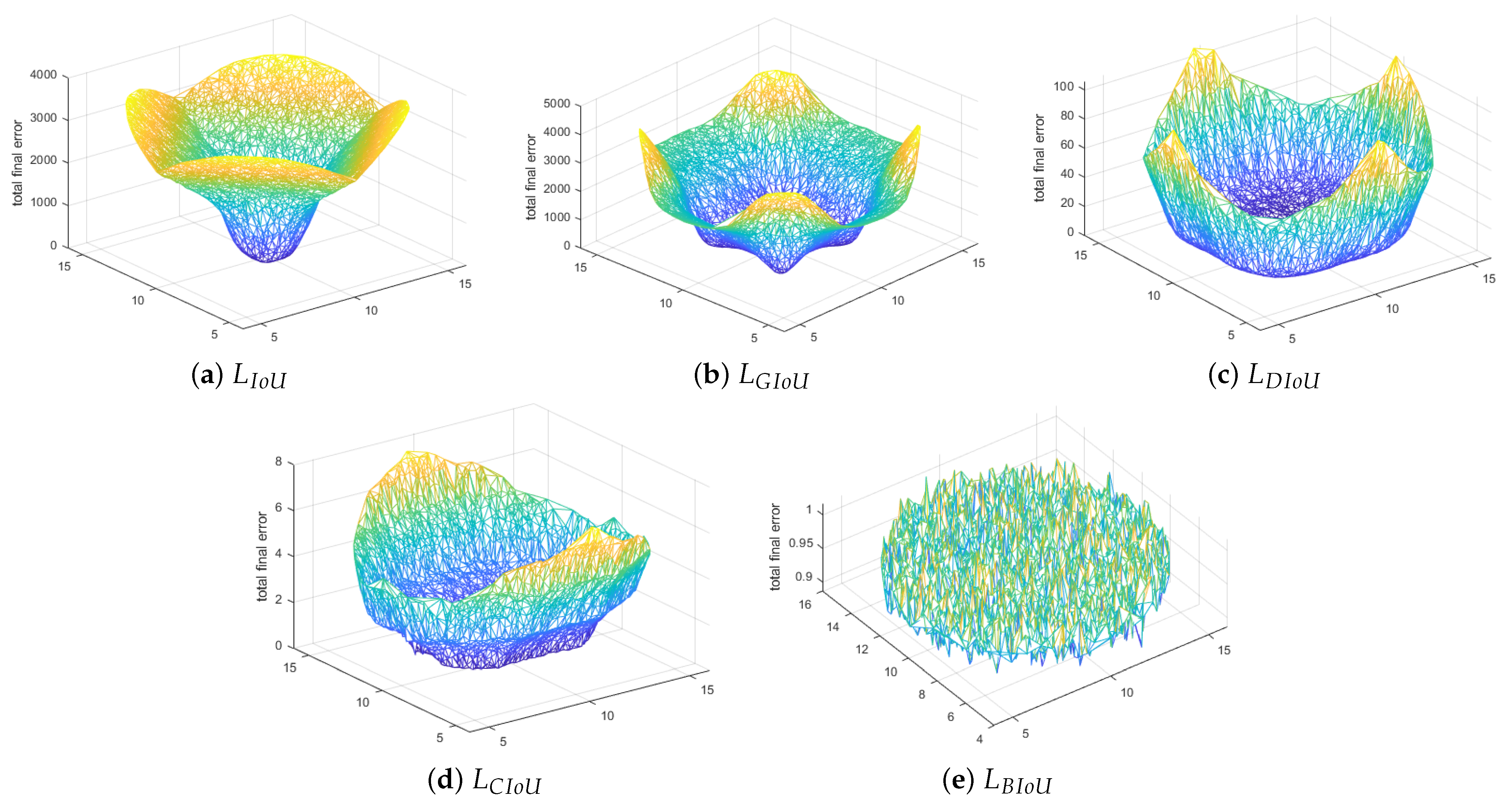
6.1. Ablation Study
- The center coordinates of the ground truth box were fixed at (10, 10). The width-to-height ratio was kept at one, and various aspect ratios were considered, such as 1:4, 1:3, 1:2, 1:1, 2:1, 3:1, and 4:1.
- Five thousand data points of uniformly distributed anchor boxes were chosen with seven aspect ratios and scales. The anchor boxes also had a similar range of aspect ratios compared to ground truths and various areas, such as 0.5, 0.67, 0.75, 1, 1.33, 1.5, and 2.
- A total of 1,715,000 (7 aspect ratios × 7 different scales × 7 different areas × 5000 data points) regression cases and 200 iterations were carried out in the simulation experiment.
6.2. Evaluation on Object Detectors
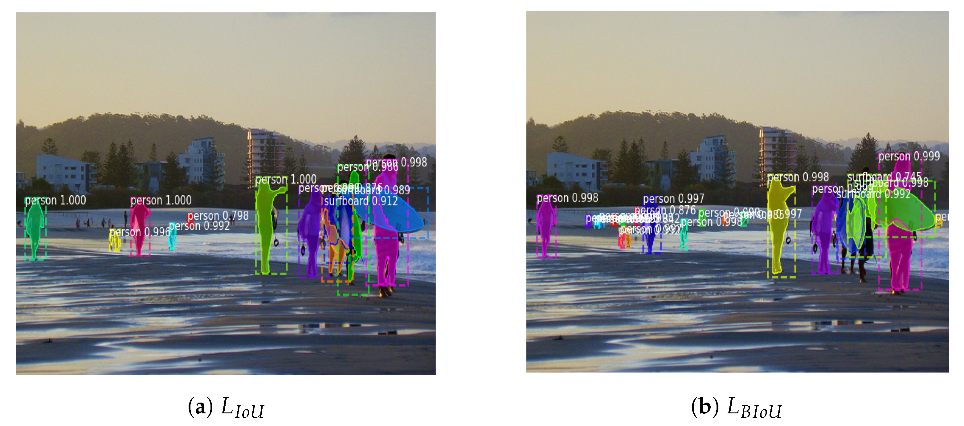
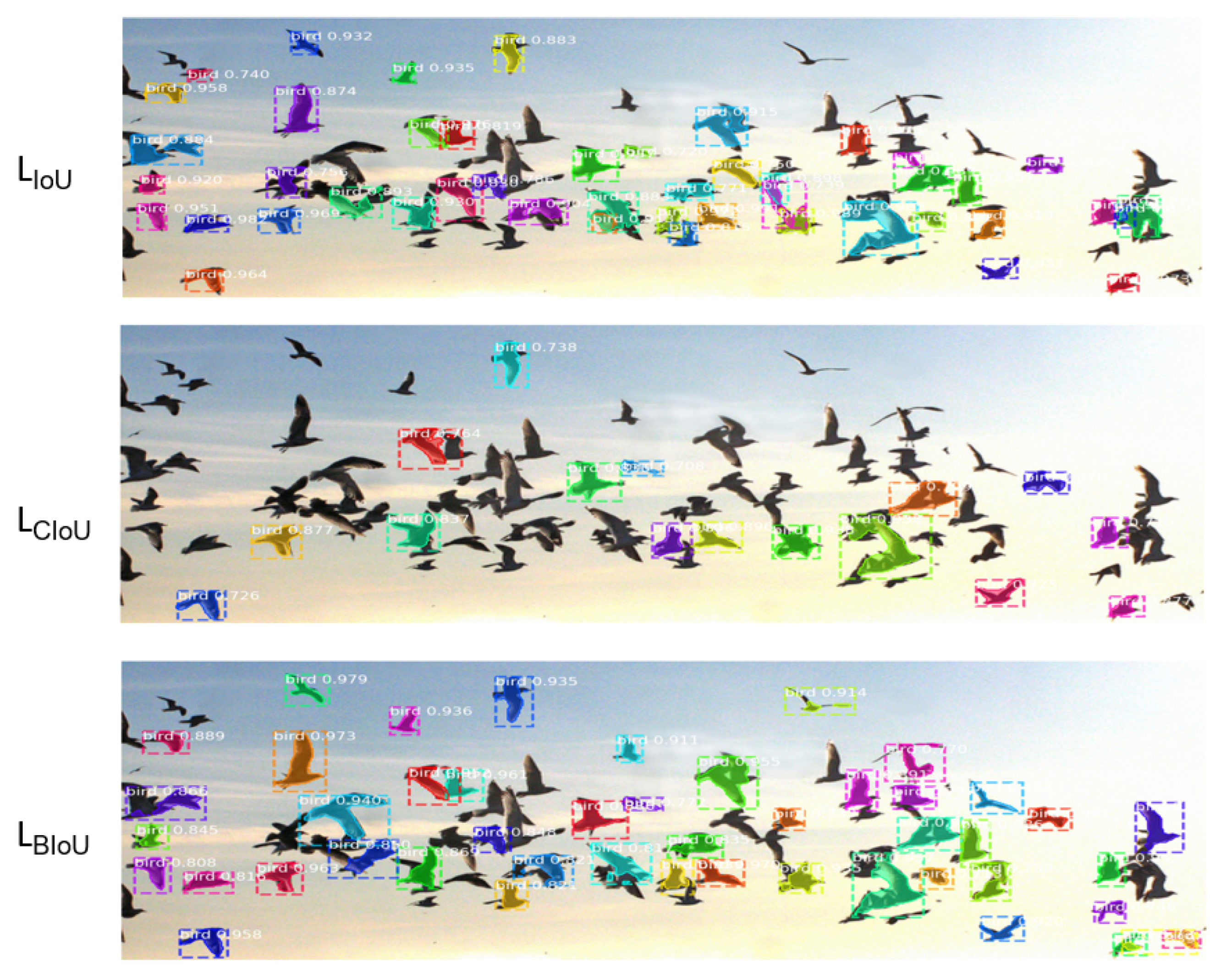
7. Performance Evaluation
Additional Observations
8. Conclusions
Author Contributions
Funding
Data Availability Statement
Conflicts of Interest
References
- Anonymous. The Automobile: Effects/Impact on Society and Changes in Cars Made by Generation—AxleAddict. 2022. Available online: https://axleaddict.com/auto-industry/Affects-of-the-Automobile-on-Society-and-Changes-Made-by-Generation (accessed on 25 July 2022).
- Chitanvis, R.; Ravi, N.; Zantye, T.; El-Sharkawy, M. Collision avoidance and Drone surveillance using Thread protocol in V2V and V2I communications. In Proceedings of the 2019 IEEE National Aerospace and Electronics Conference (NAECON), Dayton, OH, USA, 15–19 July 2019; pp. 406–411. [Google Scholar]
- Katare, D.; El-Sharkawy, M. Embedded System Enabled Vehicle Collision Detection: An ANN Classifier. In Proceedings of the 2019 IEEE 9th Annual Computing and Communication Workshop and Conference (CCWC), Las Vegas, NV, USA, 7–9 January 2019; pp. 0284–0289. [Google Scholar] [CrossRef]
- Bergek, A.; Berggren, C.; KITE Research Group. The impact of environmental policy instruments on innovation: A review of energy and automotive industry studies. Ecol. Econ. 2014, 106, 112–123. [Google Scholar] [CrossRef]
- Electric Scooters Market Size, Share & Trends Analysis Report by Product (Retro, Standing/Self-Balancing, Folding), by Battery (Sealed Lead Acid, NiMH, Li-Ion), by Voltage, and Segment Forecasts, 2022–2030. 2022. Available online: https://www.grandviewresearch.com/industry-analysis/electric-scooters-market (accessed on 25 July 2022).
- Kobayashi, L.M.; Williams, E.; Brown, C.V.; Emigh, B.J.; Bansal, V.; Badiee, J.; Checchi, K.D.; Castillo, E.M.; Doucet, J. The e-merging e-pidemic of e-scooters. Trauma Surg. Acute Care Open 2019, 4, e000337. [Google Scholar] [CrossRef] [PubMed]
- Gössling, S. Integrating e-scooters in urban transportation: Problems, policies, and the prospect of system change. Transp. Res. Part D Transp. Environ. 2020, 79, 102230. [Google Scholar] [CrossRef]
- Tuncer, S.; Brown, B. E-scooters on the ground: Lessons for redesigning urban micro-mobility. In Proceedings of the 2020 CHI Conference on Human Factors in Computing Systems, Honolulu, HI, USA, 25–30 April 2020; pp. 1–14. [Google Scholar]
- Venkitachalam, S.; Manghat, S.K.; Gaikwad, A.S.; Ravi, N.; Bhamidi, S.B.S.; El-Sharkawy, M. Realtime applications with rtmaps and bluebox 2.0. In Proceedings of the International Conference on Artificial Intelligence (ICAI), Las Vegas, NV, USA, 30 July–2 August 2018; pp. 137–140. [Google Scholar]
- Zou, Z.; Shi, Z.; Guo, Y.; Ye, J. Object detection in 20 years: A survey. arXiv 2019, arXiv:1905.05055. [Google Scholar]
- Girshick, R.; Donahue, J.; Darrell, T.; Malik, J. Rich feature hierarchies for accurate object detection and semantic segmentation. In Proceedings of the IEEE Conference on Computer Vision and Pattern Recognition, Columbus, OH, USA, 23–28 June 2014; pp. 580–587. [Google Scholar]
- Katare, D.; El-Sharkawy, M. Real-Time 3-D Segmentation on An Autonomous Embedded System: Using Point Cloud and Camera. In Proceedings of the 2019 IEEE National Aerospace and Electronics Conference (NAECON), Dayton, OH, USA, 15–19 July 2019; pp. 356–361. [Google Scholar] [CrossRef]
- Redmon, J.; Farhadi, A. Yolov3: An incremental improvement. arXiv 2018, arXiv:1804.02767. [Google Scholar]
- Redmon, J.; Divvala, S.; Girshick, R.; Farhadi, A. You only look once: Unified, real-time object detection. In Proceedings of the IEEE Conference on Computer Vision and Pattern Recognition, Las Vegas, NV, USA, 27–30 June 2016; pp. 779–788. [Google Scholar]
- Ieamsaard, J.; Charoensook, S.N.; Yammen, S. Deep learning-based face mask detection using yoloV5. In Proceedings of the 2021 9th International Electrical Engineering Congress (iEECON), Pattaya, Thailand, 10–12 March 2021; pp. 428–431. [Google Scholar]
- Liu, W.; Anguelov, D.; Erhan, D.; Szegedy, C.; Reed, S.; Fu, C.Y.; Berg, A.C. Ssd: Single shot multibox detector. In Proceedings of the European Conference on Computer Vision, Amsterdam, The Netherlands, 11–14 October 2016; pp. 21–37. [Google Scholar]
- Ren, S.; He, K.; Girshick, R.; Sun, J. Faster r-cnn: Towards real-time object detection with region proposal networks. Adv. Neural Inf. Process. Syst. 2015, 28, 1–14. [Google Scholar] [CrossRef]
- Wang, Q.; Cheng, J. LCornerIoU: An Improved IoU-based Loss Function for Accurate Bounding Box Regression. In Proceedings of the 2021 International Conference on Intelligent Computing, Automation and Systems (ICICAS), Chongqing, China, 29–31 December 2021; pp. 377–383. [Google Scholar]
- Sun, D.; Yang, Y.; Li, M.; Yang, J.; Meng, B.; Bai, R.; Li, L.; Ren, J. A scale balanced loss for bounding box regression. IEEE Access 2020, 8, 108438–108448. [Google Scholar] [CrossRef]
- Zheng, Z.; Wang, P.; Ren, D.; Liu, W.; Ye, R.; Hu, Q.; Zuo, W. Enhancing geometric factors in model learning and inference for object detection and instance segmentation. IEEE Trans. Cybern. 2022, 52, 8574–8586. [Google Scholar] [CrossRef]
- Wang, Y.; Zhao, X.; Hu, X.; Li, Y.; Huang, K. Focal boundary guided salient object detection. IEEE Trans. Image Process. 2019, 28, 2813–2824. [Google Scholar] [CrossRef]
- Lin, T.Y.; Maire, M.; Belongie, S.; Hays, J.; Perona, P.; Ramanan, D.; Dollár, P.; Zitnick, C.L. Microsoft coco: Common objects in context. In Proceedings of the European Conference on Computer Vision, Zurich, Switzerland, 6–12 September 2014; pp. 740–755. [Google Scholar]
- Goldman, E.; Herzig, R.; Eisenschtat, A.; Goldberger, J.; Hassner, T. Precise detection in densely packed scenes. In Proceedings of the IEEE/CVF Conference on Computer Vision and Pattern Recognition, Long Beach, CA, USA, 15–20 June 2019; pp. 5227–5236. [Google Scholar]
- Vidhya, C.B.A. Evolution of Object Detection. 2020. Available online: https://medium.com/analytics-vidhya/evolution-of-object-detection-582259d2aa9b (accessed on 25 July 2022).
- Dalal, N.; Triggs, B. Histograms of oriented gradients for human detection. In Proceedings of the 2005 IEEE Computer Society Conference on Computer Vision and Pattern Recognition (CVPR’05), San Diego, CA, USA, 20–26 June 2005; Volume 1, pp. 886–893. [Google Scholar] [CrossRef]
- Girshick, R.; Iandola, F.; Darrell, T.; Malik, J. Deformable part models are convolutional neural networks. In Proceedings of the IEEE Conference on Computer Vision and Pattern Recognition, Boston, MA, USA, 7–12 June 2015; pp. 437–446. [Google Scholar]
- Mallick, S. Histogram of Oriented Gradients Explained Using OpenCV. 2016. Available online: https://learnopencv.com/histogram-of-oriented-gradients/ (accessed on 26 July 2022).
- Girshick, R. Fast r-cnn. In Proceedings of the IEEE International Conference on Computer Vision, Santiago, Chile, 7–13 December 2015; pp. 1440–1448. [Google Scholar]
- Dwivedi, P. YOLOv5 Compared to Faster RCNN. Who Wins? 2020. Available online: https://towardsdatascience.com/yolov5-compared-to-faster-rcnn-who-wins-a771cd6c9fb4 (accessed on 27 July 2022).
- Redmon, J.; Farhadi, A. YOLO9000: Better, faster, stronger. In Proceedings of the IEEE Conference on Computer Vision and Pattern Recognition, Honolulu, HI, USA, 21–26 July 2017; pp. 7263–7271. [Google Scholar]
- Zheng, Z.; Wang, P.; Liu, W.; Li, J.; Ye, R.; Ren, D. Distance-IoU loss: Faster and better learning for bounding box regression. In Proceedings of the AAAI Conference on Artificial Intelligence, New York, NY, USA, 7–8 February 2020; Volume 34, pp. 12993–13000. [Google Scholar]
- Wang, G.; Zhuang, Y.; Chen, H.; Liu, X.; Zhang, T.; Li, L.; Dong, S.; Sang, Q. FSoD-Net: Full-scale object detection from optical remote sensing imagery. IEEE Trans. Geosci. Remote Sens. 2021, 60, 1–18. [Google Scholar] [CrossRef]
- Cheng, G.; Si, Y.; Hong, H.; Yao, X.; Guo, L. Cross-scale feature fusion for object detection in optical remote sensing images. IEEE Geosci. Remote Sens. Lett. 2020, 18, 431–435. [Google Scholar] [CrossRef]
- Deng, Z.; Sun, H.; Zhou, S.; Zhao, J.; Lei, L.; Zou, H. Multi-scale object detection in remote sensing imagery with convolutional neural networks. ISPRS J. Photogramm. Remote Sens. 2018, 145, 3–22. [Google Scholar] [CrossRef]
- Bao, S.; Zhong, X.; Zhu, R.; Zhang, X.; Li, Z.; Li, M. Single shot anchor refinement network for oriented object detection in optical remote sensing imagery. IEEE Access 2019, 7, 87150–87161. [Google Scholar] [CrossRef]
- Xu, Z.; Xu, X.; Wang, L.; Yang, R.; Pu, F. Deformable convnet with aspect ratio constrained nms for object detection in remote sensing imagery. Remote Sens. 2017, 9, 1312. [Google Scholar] [CrossRef]
- Hong, D.; Gao, L.; Yao, J.; Zhang, B.; Plaza, A.; Chanussot, J. Graph convolutional networks for hyperspectral image classification. IEEE Trans. Geosci. Remote Sens. 2020, 59, 5966–5978. [Google Scholar] [CrossRef]
- Wu, X.; Hong, D.; Tian, J.; Chanussot, J.; Li, W.; Tao, R. ORSIm detector: A novel object detection framework in optical remote sensing imagery using spatial-frequency channel features. IEEE Trans. Geosci. Remote Sens. 2019, 57, 5146–5158. [Google Scholar] [CrossRef]
- Hong, D.; Gao, L.; Yokoya, N.; Yao, J.; Chanussot, J.; Du, Q.; Zhang, B. More diverse means better: Multimodal deep learning meets remote-sensing imagery classification. IEEE Trans. Geosci. Remote Sens. 2020, 59, 4340–4354. [Google Scholar] [CrossRef]
- Hong, D.; Yokoya, N.; Chanussot, J.; Zhu, X.X. An augmented linear mixing model to address spectral variability for hyperspectral unmixing. IEEE Trans. Image Process. 2018, 28, 1923–1938. [Google Scholar] [CrossRef]
- Hang, R.; Li, Z.; Ghamisi, P.; Hong, D.; Xia, G.; Liu, Q. Classification of hyperspectral and LiDAR data using coupled CNNs. IEEE Trans. Geosci. Remote Sens. 2020, 58, 4939–4950. [Google Scholar] [CrossRef]
- Yu, J.; Jiang, Y.; Wang, Z.; Cao, Z.; Huang, T. Unitbox: An advanced object detection network. In Proceedings of the 24th ACM International Conference on Multimedia, Amsterdam, The Netherlands, 15–19 October 2016; pp. 516–520. [Google Scholar]
- Rezatofighi, H.; Tsoi, N.; Gwak, J.; Sadeghian, A.; Reid, I.; Savarese, S. Generalized intersection over union: A metric and a loss for bounding box regression. In Proceedings of the IEEE/CVF Conference on Computer Vision and Pattern Recognition, Long Beach, CA, USA, 15–20 June 2019; pp. 658–666. [Google Scholar]
- Zhang, Y.F.; Ren, W.; Zhang, Z.; Jia, Z.; Wang, L.; Tan, T. Focal and efficient IOU loss for accurate bounding box regression. arXiv 2021, arXiv:2101.08158. [Google Scholar] [CrossRef]
- Wang, X.; Song, J. ICIoU: Improved loss based on complete intersection over union for bounding box regression. IEEE Access 2021, 9, 105686–105695. [Google Scholar] [CrossRef]
- Du, S.; Zhang, B.; Zhang, P.; Xiang, P. An Improved Bounding Box Regression Loss Function Based on CIOU Loss for Multi-scale Object Detection. In Proceedings of the 2021 IEEE 2nd International Conference on Pattern Recognition and Machine Learning (PRML), Chengdu, China, 16–18 July 2021; pp. 92–98. [Google Scholar]
- Du, S.; Zhang, B.; Zhang, P. Scale-Sensitive IOU Loss: An Improved Regression Loss Function in Remote Sensing Object Detection. IEEE Access 2021, 9, 141258–141272. [Google Scholar] [CrossRef]
- Wu, S.; Yang, J.; Wang, X.; Li, X. Iou-balanced loss functions for single-stage object detection. Pattern Recognit. Lett. 2022, 156, 96–103. [Google Scholar] [CrossRef]
- Zhang, H.; Wang, Y.; Dayoub, F.; Sunderhauf, N. Varifocalnet: An iou-aware dense object detector. In Proceedings of the IEEE/CVF Conference on Computer Vision and Pattern Recognition, Nashville, TN, USA, 19–25 June 2021; pp. 8514–8523. [Google Scholar]
- Chen, Z.; Chen, K.; Lin, W.; See, J.; Yu, H.; Ke, Y.; Yang, C. Piou loss: Towards accurate oriented object detection in complex environments. In Proceedings of the European Conference on Computer Vision, Glasgow, UK, 23–28 August 2020; pp. 195–211. [Google Scholar]
- Zhou, D.; Fang, J.; Song, X.; Guan, C.; Yin, J.; Dai, Y.; Yang, R. Iou loss for 2d/3d object detection. In Proceedings of the 2019 International Conference on 3D Vision (3DV), Quebec City, QC, Canada, 16–19 September 2019; pp. 85–94. [Google Scholar]
- Yang, X.; Yan, J.; Ming, Q.; Wang, W.; Zhang, X.; Tian, Q. Rethinking rotated object detection with gaussian wasserstein distance loss. In Proceedings of the International Conference on Machine Learning, Virtual, 18–24 July 2021; pp. 11830–11841. [Google Scholar]
- Ravi, N.; El-Sharkawy, M. Real-Time Embedded Implementation of Improved Object Detector for Resource-Constrained Devices. J. Low Power Electron. Appl. 2022, 12, 21. [Google Scholar] [CrossRef]
- He, K.; Gkioxari, G.; Dollár, P.; Girshick, R. Mask r-cnn. In Proceedings of the IEEE International Conference on Computer Vision, Venice, Italy, 22–29 October 2017; pp. 2961–2969. [Google Scholar]
- Hu, D. An introductory survey on attention mechanisms in NLP problems. In Proceedings of the SAI Intelligent Systems Conference, London, UK, 5–6 September 2019; pp. 432–448. [Google Scholar]
- Abdulla, W. Mask R-CNN for Object Detection and Instance Segmentation on Keras and TensorFlow. 2017. Available online: https://github.com/matterport/Mask_RCNN (accessed on 20 July 2022).
- Everingham, M.; Van Gool, L.; Williams, C.K.; Winn, J.; Zisserman, A. The pascal visual object classes (voc) challenge. Int. J. Comput. Vis. 2010, 88, 303–338. [Google Scholar] [CrossRef]
- Kalgaonkar, P.; El-Sharkawy, M. Condensenext: An ultra-efficient deep neural network for embedded systems. In Proceedings of the 2021 IEEE 11th Annual Computing and Communication Workshop and Conference (CCWC), Las Vegas, NV, USA, 27–30 January 2021; pp. 0524–0528. [Google Scholar]


| Loss Eval | AP50:95 | AP50 | AP75 | |||
|---|---|---|---|---|---|---|
| 20.2 | 35.5 | 21.1 | 6.2 | 24.8 | 34.2 | |
| 22.0 | 41.6 | 21.7 | 8.9 | 25.9 | 34.5 | |
| A.I% | 1.80 | 6.10 | 0.59 | 2.70 | 1.09 | 0.29 |
| 20.8 | 40.6 | 19.3 | 9.3 | 27.3 | 31.0 | |
| A.I% | 0.60 | 5.10 | −1.80 | 3.10 | 2.50 | −3.20 |
| 21.7 | 40.7 | 21.9 | 10.2 | 25.8 | 33.7 | |
| A.I% | 1.50 | 5.20 | 0.79 | 3.99 | 1.0 | −0.5 |
| 22.3 | 41.5 | 22.2 | 9.9 | 27.7 | 33.00 | |
| A.I% | 2.10 | 6.00 | 1.09 | 3.70 | 2.89 | −1.20 |
| Loss Eval | AP50 | AP55 | AP60 | AP65 | AP70 | AP75 | AP80 | AP85 | AP90 | AP95 |
|---|---|---|---|---|---|---|---|---|---|---|
| 75.00 | 70.90 | 66.20 | 60.00 | 51.10 | 38.60 | 23.30 | 9.44 | 2.20 | 1.40 | |
| 72.50 | 68.60 | 64.10 | 58.00 | 49.40 | 37.50 | 22.90 | 9.33 | 2.16 | 1.23 | |
| R.L% | −3.33 | −3.24 | −3.17 | −3.33 | −3.32 | −2.85 | −1.71 | −0.74 | −1.81 | −12.1 |
| 73.50 | 69.60 | 65.00 | 58.80 | 50.00 | 38.00 | 23.00 | 9.30 | 2.16 | 1.10 | |
| R.L% | −2.00 | −1.83 | −1.81 | −2 | −2.15 | −1.55 | −1.28 | −1.06 | −1.81 | −21.4 |
| 73.70 | 69.60 | 64.90 | 58.80 | 50.20 | 38.00 | 23.10 | 9.44 | 2 | 1.20 | |
| R.L% | −1.73 | −1.83 | −1.96 | −2.00 | −1.76 | −1.55 | −0.85 | 0.42 | −9.09 | −14.2 |
| 79.40 | 75.30 | 70.10 | 63.00 | 53.20 | 39.90 | 24.00 | 9.69 | 2.22 | 1.16 | |
| R.L% | 5.86 | 6.20 | 5.89 | 5.00 | 4.10 | 3.36 | 3.00 | 3.08 | 0.909 | −17.1 |
| Loss Eval | AP50 | AP55 | AP60 | AP65 | AP70 | AP75 | AP80 | AP85 | AP90 | AP95 |
|---|---|---|---|---|---|---|---|---|---|---|
| 89.80 | 89.50 | 87.90 | 85.80 | 82.20 | 72.90 | 63.10 | 37.20 | 6.47 | 0.06 | |
| 91.00 | 89.40 | 88.60 | 85.10 | 83.60 | 78.70 | 66.50 | 32.20 | 7.73 | 1.08 | |
| R.L% | 1.33 | −0.11 | 0.79 | −0.81 | 1.70 | 7.96 | 5.38 | −13.4 | 19.47 | 17.00 |
| 89.60 | 87.40 | 84.80 | 82.80 | 79.90 | 73.40 | 63.00 | 32.70 | 5.53 | 1.20 | |
| R.L% | −0.22 | −2.34 | −3.52 | −3.49 | −2.79 | 0.68 | −0.16 | −12.1 | −14.5 | 19.00 |
| 90.90 | 90.10 | 87.80 | 86.40 | 82.40 | 75.70 | 61.50 | 28.00 | 3.70 | 1.60 | |
| R.L% | 1.22 | 0.67 | −0.11 | 0.69 | 0.24 | 3.84 | −2.5 | −24.7 | −42.8 | 25.7 |
| 91.80 | 89.10 | 86.20 | 84.30 | 82.50 | 77.10 | 68.80 | 38.20 | 7.72 | 1.70 | |
| R.L% | 2.22 | −0.44 | −1.93 | −1.74 | 0.36 | 5.76 | 9.03 | 2.68 | 19.31 | 27.3 |
Publisher’s Note: MDPI stays neutral with regard to jurisdictional claims in published maps and institutional affiliations. |
© 2022 by the authors. Licensee MDPI, Basel, Switzerland. This article is an open access article distributed under the terms and conditions of the Creative Commons Attribution (CC BY) license (https://creativecommons.org/licenses/by/4.0/).
Share and Cite
Ravi, N.; Naqvi, S.; El-Sharkawy, M. BIoU: An Improved Bounding Box Regression for Object Detection. J. Low Power Electron. Appl. 2022, 12, 51. https://doi.org/10.3390/jlpea12040051
Ravi N, Naqvi S, El-Sharkawy M. BIoU: An Improved Bounding Box Regression for Object Detection. Journal of Low Power Electronics and Applications. 2022; 12(4):51. https://doi.org/10.3390/jlpea12040051
Chicago/Turabian StyleRavi, Niranjan, Sami Naqvi, and Mohamed El-Sharkawy. 2022. "BIoU: An Improved Bounding Box Regression for Object Detection" Journal of Low Power Electronics and Applications 12, no. 4: 51. https://doi.org/10.3390/jlpea12040051
APA StyleRavi, N., Naqvi, S., & El-Sharkawy, M. (2022). BIoU: An Improved Bounding Box Regression for Object Detection. Journal of Low Power Electronics and Applications, 12(4), 51. https://doi.org/10.3390/jlpea12040051