Abstract
Object detection is a predominant challenge in computer vision and image processing to detect instances of objects of various classes within an image or video. Recently, a new domain of vehicular platforms, e-scooters, has been widely used across domestic and urban environments. The driving behavior of e-scooter users significantly differs from other vehicles on the road, and their interactions with pedestrians are also increasing. To ensure pedestrian safety and develop an efficient traffic monitoring system, a reliable object detection system for e-scooters is required. However, existing object detectors based on IoU loss functions suffer various drawbacks when dealing with densely packed objects or inaccurate predictions. To address this problem, a new loss function, balanced-IoU (BIoU), is proposed in this article. This loss function considers the parameterized distance between the centers and the minimum and maximum edges of the bounding boxes to address the localization problem. With the help of synthetic data, a simulation experiment was carried out to analyze the bounding box regression of various losses. Extensive experiments have been carried out on a two-stage object detector, MASK_RCNN, and single-stage object detectors such as YOLOv5n6, YOLOv5x on Microsoft Common Objects in Context, SKU110k, and our custom e-scooter dataset. The proposed loss function demonstrated an increment of 3.70% at on the COCO dataset, 6.20% at AP55 on SKU110k, and 9.03% at AP80 of the custom e-scooter dataset.
1. Introduction
The automotive industry plays a vital role in shaping human transportation history [1,2]. The motor industry has evolved exponentially since the introduction of two-wheel drive to the latest self-driving cars [3]. However, at the same time, pollution, traffic, and parking are major problems in the urban environment caused by motorized vehicles [4]. Urban transport planners have embraced e-scooters as a disruptive innovation with the potential to reshape the urban mobility system and conquer the last mile. The global electric scooter market size was broadly evaluated at USD 19.4 billion in 2021, and the market is expected to grow further [5]. E-scooters are manufactured to travel at a maximum speed of 15 to 17 miles per hour (24–28 km/h), complicating the traffic rules [6]. They also pose challenges for urban transport planners to design effective regulation for the growing alternative transportation system [7,8]. The interaction of pedestrians and e-scooters has introduced concerns over speed, safety, and user behavior, and e-scooters contest over pedestrian and cyclist spaces. Additionally, the lack of infrastructure for driving and parking e-scooters leads to users as well as independent contractors scattering the e-scooters on pavements or sidewalks, which obstructs the path designated for pedestrians and bicycles and exposes the physically challenged to a greater risk of accident due to safety issues raised by e-scooters driven on pavements [7]. E-scooters are generally smaller than cars and motorbikes, and identification/detection of e-scooters is a difficult challenge. To solve these problems, traffic monitoring systems with efficient algorithms are required to detect e-scooters.
In recent years, computer vision (CV) algorithms have been widely used in the autonomous and automotive industry [9]. There are several computer vision applications, such as image classification, object detection, and image segmentation. Object detection is a fundamental challenge of computer vision since it shapes the basis for computer vision tasks like instance segmentation, object tracking, and image captioning [10,11,12]. Most computer vision tasks do not demand a very significant degree of accuracy, so it is a rational thought to trade off accuracy for faster-to-train methods [13]. In 2015, R. Joseph et al. introduced a single-stage object detector model, You Only Look Once (YOLO), which has demonstrated a peak performance as compared to other object detection networks such as DPM (Deformable Part Models) and R-CNN (Region-based Convolutional Neural Network) [14]. Various deep learning and computer vision applications have recently used YOLO networks owing to their smaller network size and higher performance [15]. Bounding box regression is crucial in almost all object detection and tracking algorithms. Bounding box regression rectifies the predicted bounding box, which helps facilitate locating the targeted object. Most of the popular object detectors, like the SSD [16], Faster R-CNN [17], and YOLOv3 [13] use normalization loss to calculate the overall localization errors [18]. The disadvantage of using -norm based loss is an undesired increase in regression loss as the proportions of the bounding boxes expand, even if their relative position is not altered [19]. Object detection models like YOLOv3 and Faster R-CNN achieve better precision using Generalized IoU (GIoU) loss instead of -norm-based losses [20].
During bounding box regression, the state-of-art IoU-based loss functions suffer various drawbacks such as poor convergence and incorrect regression [21]. This research focuses on developing an efficient object detector model by addressing drawbacks in existing IoU-based loss functions and evaluating the performance in COCO [22], an e-scooter dataset and SKU110K [23]. The organization of the research article is explained briefly in this section.
- The research begins with a background study on object detection and bounding box regression losses in Section 2.
- Section 5 provides an overview of the datasets utilized in this research study.
- Simulation experiments and their results are detailed in Section 6.1.
- Section 6.2 provides background on the experimental setup and deep learning architecture chosen for this research.
- The performance of the proposed BIoU loss is evaluated in Section 7.
2. Literature Review
2.1. Object Detection
The main function of object detection is to discover all the targets of interest from the given input image, classify the targeted objects, and utilize bounding boxes for positioning. Detecting such various objects in so many different conditions brings new challenges. Object detection can be split into two categories, namely, the traditional object detection period (before year 2014) and the deep-learning-based detection period (after year 2014) [10,24]. Some of the famous object detectors from the traditional object detection period (before the year 2014) are the Histogram of Oriented Gradients (HOG) detector [25] and the improved Deformable Part Model Detector (DPM) detector [26]. The HOG detector was originally proposed in 2005, an upgrade of the scale-invariant feature transform methods of its time. HOGs are well known for their initial implementation in detecting pedestrians [27]. Deep-learning-based object detection methods can be broadly divided into two categories: two-stage algorithms and single-stage algorithms. Various two-stage object detectors, such as RCNN [11], Fast R-CNN [28], and Faster R-CNN [17], utilize a regional proposal network (RPN), where the candidate regions are realized, and subsequently, these regions are classified by the neural network. A Faster R-CNN network achieved 48.4% mAP on the COCO validation set by replacing the VGG-16 backbone layer with ResNet-101 and 73.2% on the PASCAL VOC datasets. Experimental results from two-stage object detectors demonstrated superior performance compared to traditional object detectors. However, the two-stage detectors were computationally expensive and unsuitable for real-time implementation.
To address these issues, single-stage object detectors were introduced [16]. There are two prominent single-stage algorithms: YOLO [14] and the Single Shot detector (SSD) [16], both of which rely on convolutional neural networks to extract useful features and predict categories and positions. An SSD network was able to achieve 77.2% mAP on the PASCAL VOC dataset and 46.5% on the COCO test-dev dataset [16]. The single-stage algorithms have the advantage of fast detection rates but at the expense of precision. Faster inference speeds while maintaining comparatively similar performance to the RCNN algorithms gives YOLO an edge over other trending object detection neural networks [29]. Since the launch of its initial version in 2016, the YOLO network has evolved over the period of time. Batch normalization, higher resolution, and the concept of anchor boxes were introduced in YOLOv2 [30]. YOLOv2 outperformed other architectures by running faster and maintaining high accuracy simultaneously. In YOLOv3, an objectness score was introduced to enhance the bounding box prediction, and predictions were carried out at separate levels to improve the performance in detecting smaller objects [13]. YOLOv5 is one of the latest developments in the YOLO family, offering different models such as YOLOv5n (nano), YOLOv5s (small), YOLOv5m (medium), and YOLOv5l (large).
The trending deep learning object detection methods involve performing two tasks:
- Loss functions to find the bounding box coordinates to localize target objects;
- Classification to identify the target object;
- The first task relies on the loss functions, which give the error between the predicted and ground truth bounding box [31].
2.2. Remote Sensing
In recent years, many research activities have been carried out to utilize one- and two-stage object detectors in remote sensing. However, this poses a myriad of challenges since the optical remote sensing images significantly differ from natural scenes [32]. Since most optical images are captured from UAVs or satellites from an aerial view, optical images contain many degrees of deformation, scale variation, dynamic orientation, and occlusion [33]. In this research [34], the drawbacks of faster region-based convolutional neural networks (FRCN) were addressed with large-scale variability and concatenation modules. Ref. [35] addressed these challenges by regressing the multilevel features of the backbone layers to regress the offsets between the anchors and ground truths. This refinement of anchors aids in improving the model performance. In [36], aspect-ratio-constrained non-maximum suppression (arcNMS) was utilized to reduce the noise in very-high-resolution (VHR) remote sensing images.
Recently, graph theory has been utilized to establish the relationships between objects in the form of pixels. melshark@iupui.edu [37] explored different approaches to fuse CNN and GCN network layers to improve the classification model. With the help of the fusion technique, graph convolution networks (GCN) are currently utilized to provide classification in hyperspectral (HSI) images. For geospatial object detection applications, Ref. [38] extracted channel features from spatial frequencies. Various fusion architectures were studied and fused to generate a multi-model deep learning (MDL) framework [39]. In addition to pixel-wise information, spatial information is also being utilized with CNN layers in MDL. Ref. [40] addressed the problems in hyperspectral imagery by considering various spectral variability in addition to the principal scaling factor. However, many complex objects exist in urban and rural areas, and identifying individual objects brings additional challenges since the objects may have similar spectral responses. The authors of this research [41] proposed the usage of LiDAR sensors to obtain elevation information of objects followed by classification/detection tasks. Infrared (IR) camera images can be studied for 3D fusion with LiDAR data points to enrich the available information further.
2.3. Bounding Box Regression Loss
The well-known object detection and tracking methods predominantly use -norm loss for bounding box regression, but this is not customized to adapt to the evaluation metric, i.e., the intersection over union (IoU) [18]. In response, IoU loss [42] was proposed to favor the IoU metric, while focal loss [21] takes a different approach by addressing class imbalance and prohibiting the easy negatives from overwhelming the model by training on a sparse set of hard examples. Meanwhile, the generalized IoU (GIoU) [43] algorithm resolved the bounding box regression issue for situations when the bounding boxes of the ground truth and prediction do not overlap. Hence, GIoU improved the IoU loss function as IoU does not reflect the proximity of two shapes. However, the IoU and GIoU losses had slow convergence and inaccurate regression, whereas the Distance-IoU (DIoU) loss [31] combines the normalized distance in-between the predicted box and the target box, which converges much faster in training. Other notable loss functions such as the CIOU [31] achieve improved performance over their predecessors by merging three geometric components, overlap area, central point distance, and aspect ratio, which influence the regression loss value calculation. While efficient IOU loss (EIoU) improved the convergence speed and localization accuracy significantly, Focal EIoU [44] modified the parameter used to evaluate the consistency of the indispensable aspect ratio between the predicted and real boundary boxes to enhance performance further.
Meanwhile, the ICIoU [45] refined the localization accuracy and bounding box regression by including a penalty function that uses the ratio of the corresponding width and height of the bounding box for the given ground truth and the calculated prediction. Another attempt to improve the CIoU loss function was scale-sensitive IoU (SIoU) [46], which aimed to differentiate all the estimated bounding boxes in theory and enhance the overall optimization procedure. SIoU introduced an additional geometric factor, area-difference, when calculating the regression loss values to generate a more reasonable calculation. Additionally, SIoU improved the accuracy of multi-scale object detection in the conventional bounding box and the oriented bounding box for broader applicability. A recent improvement to the IoU-based loss function is LCornerIoU [18], which normalized the corner distance and parameterized the width-height difference penalty term to boost the prediction of the boundary box position. Ref. [47] considered the area difference between the boxes to increase the optimal performance. To improve the correlation between classification and localization loss, IoU-balance [48] loss assigns higher weights for positive samples with high IoU. This significantly increases localization accuracy but does not improve the classification loss [49]. PIoU maximizes the relationship between angle error and IoU of two oriented bounding boxes [50]. In this research, IoU [51] is computed for two rotated bounding boxes for 3D bounding boxes. Ref. [52] utilizes the Gaussian Wasserstein distance to optimize the bounding box regression problem. Ref. [19] proposes an asymmetry of loss function based on the IoU metric. When the boxes do not overlap, the proposed loss function also suffers from a symmetry trap since it does not account for the aspect ratio of the boxes. This would account for the same value of the loss function even if the boxes are altered in their position.
3. Survey on Axis-Aligned Loss Functions
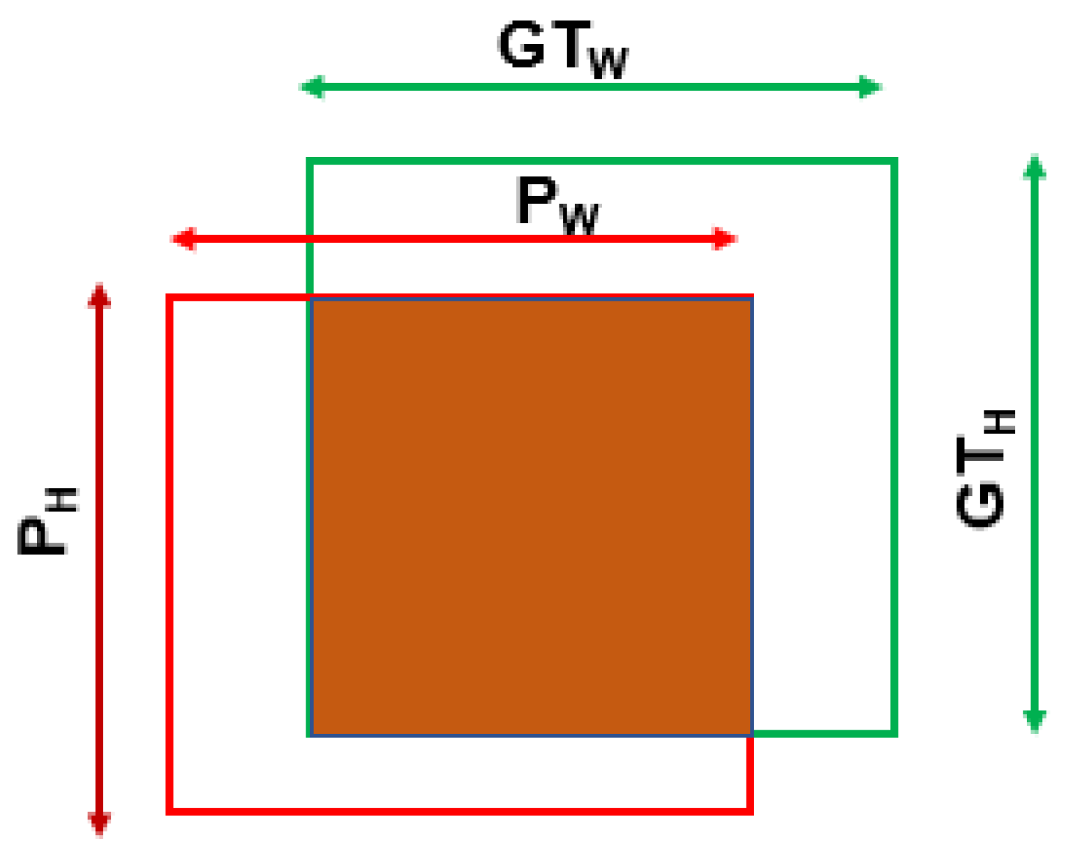
This section details a survey on existing loss functions for axis-aligned object detection. During the training phase of the object detector, bounding box regression (BBR) calculates the loss between ground truth, , and predictions developed by the neural network model, . Bounding boxes are rectangular and are mathematically represented by (x, y, w, h), where x and y represent the centers of the x and y-axis. In contrast, w and h represent the height and width of the box, as shown in Figure 1. The objective of an object detector is to refine the during training phase to match by calculating the offsets (, , , ) between (, , , ) and (, , , ). The offsets are calculated as follows:
These sections briefly describe various IoU functions utilized to optimize the regression of bounding boxes.
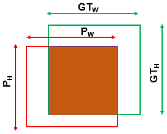
Figure 1.
Sample relationships between ground truth (blue) and prediction boxes (red).
IoU executes a simple approach in estimating the intersection/overlap regions between and . The overlap region is calculated as the IoU area. The mathematical formula for the loss equation of the IoU loss is expressed as
However, the IoU fails to converge when boxes do not overlap. GIoU loss addresses these shortcomings by considering a convex region proposed as
where C indicates the minimum convex region enclosing both prediction and ground truth boxes. This approach considers the entire area between the boxes and provides better loss convergence, even in non-overlapping cases.
From Equation (5), we can observe that the intersection area is the deciding factor in estimating the IoU loss. There could be various cases in which predictions developed by the network are located far away from the ground truth or cases where they are closer but do not overlap. During these cases, , becomes 1, indicating a very high loss for the prediction. Additionally, the training dataset would contain various objects of different scales, sizes, areas, and aspect ratios. For instance, two cases, one where the prediction box is smaller than the ground truth, and the second where the ground truth is smaller than the prediction, might have the same overlap and corresponding ranging between 0 and 1. This loss provides no additional information in the above cases and affects the network convergence rate.
The GIoU loss function addresses the drawbacks of IoU when there is no overlap between the boxes. A minimum convex area, C, enclosing both the prediction and ground truth boxes, is considered. The ratio of the area difference between C and would provide an additional penalty term in loss estimation and helps the network to regress faster. However, in the cases of complete inclusion, GIoU degrades to the IoU because the C equals . As a result, network convergence is still affected.
The DIoU and CIoU loss have been recently proposed to overcome the shortcomings of IoU and GIoU losses [31]. DIoU loss overcomes the drawbacks of IoU and GIoU by carefully estimating the distance between the centers of two rectangles. c in (7) is the diagonal distance of the convex area enclosing the two boxes.
In addition, aspect ratios can also be considered for better regression. CIoU provides one step further in considering the aspect ratio of the width and height of the boxes.
In general, DIoU and CIoU seem to address the shortcomings of IoU and GIoU losses, but they also face drawbacks. From (7) and (8), we can observe that the distance between the centers plays a crucial role in loss estimation. However, in the event of inclusion and centers aligned with each other, DIoU degrades to IoU loss. This leads to poor loss estimation. CIoU losses exhibit the same behavior, where it highly depends upon the parameter from (9) and the aspect ratio of width and height of the boxes are considered. However, the width and height of ground truth could also be similar to the ratio of the prediction box, even when the prediction box is smaller or larger. This would lead to cases where = , thus making the 0.
4. Proposed BIoU Loss Function
In this research, we propose an enhanced loss function by considering the distance between the central regions and edges of the boxes as
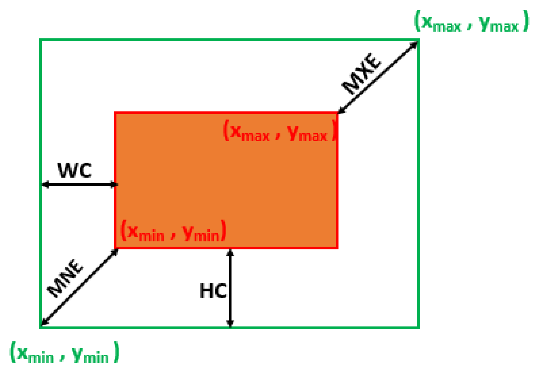
indicates the regression loss estimation between the ground truth and prediction box values. To address the drawbacks of the IoU, GIoU, DIoU and CIoU losses, the proposed loss function considers four different geometric factors to solve the bounding box regression problem. In (11), WC and HC represent the distance between the centers of the x- and y-axis of the boxes with a balance factor . estimates the width and height ratio of and and is multiplied with WC and HC values. This factor controls the regression rate of bounding boxes and prevents gradient explosion. MNE and MXE represent the distance between minimum and maximum edges of and , displayed in Figure 2. MNE and MXE are calculated by estimating the Euclidean distance between (, ) points and (, ) coordinates of the ground truth and prediction boxes. Our previous work [53] addresses the stability of considering WC and HC, and consideration of with MNE and MXE aids in stable convergence.

Figure 2.
The geometric representation of the distance between the centers and corners of prediction and ground truth boxes. MNE and MXE indicate the minimum and maximum edges of the boxes and are diagonally located opposite each other. The distance between the central regions is indicated by WC and HC diagonals.
To provide further understanding and observe the differences between proposed and existing ones, Figure 3 can be utilized. Figure 3a presents a scenario where the bounding boxes have the same centres and same aspect ratio and one of the boxes is inclusive to another. In this state, there is a convex area equal union area, and so → 0. Since the distance between the centres equals zero, → 0. Additionally, the boxes have same aspect ratio, , causing v → 0. This causes GIoU, DIoU and CIoU to degrade to IoU. However, the proposed loss addresses the above drawbacks by examining the distance between centres and edges individually and calculates the loss value between the boxes. Similar reasoning could be observed in Figure 3d. In Figure 3b, the boxes have the same aspect ratios, leading the CIoU to degrade to DIoU, and in Figure 3c, the same centers degrade DIoU to IoU. However, in all cases, the loss value calculated by the proposed method is higher than others, which would help reduce the regression errors and minimize the loss values even in difficult cases. An ablation study has been carried out in Section 6.1 to visualize the performance of different loss functions.
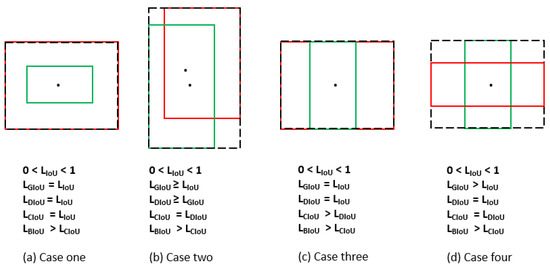
Figure 3.
Loss estimation between ground truth and prediction boxes across various loss functions. The green colored box indicates the ground truth, and the red box indicates the prediction box. The convex area is represented by a dotted line.
5. DataSet Preparation
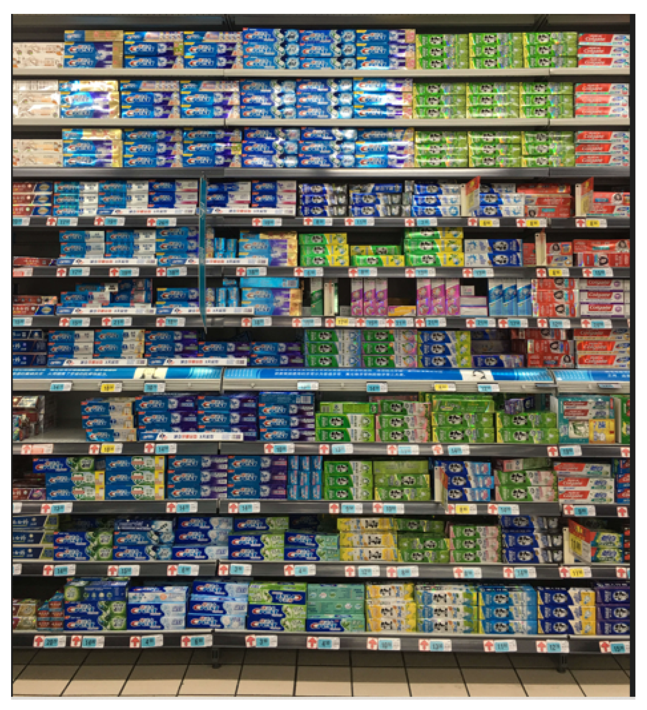
Developing neural network models that learn specific features about a target object is crucial to making computer vision applications possible. With the rapid increase in data volume, this practice of gaining insights from data has increased the popularity of supervised machine learning in recent years. This research uses multiple datasets, including the COCO (2015), SKU-110k dataset [23] and a custom dataset consisting of over 600 unprocessed images of e-scooters in natural settings. The variety of datasets provides the network with good quality training samples to improve its accuracy. A brief description of the dataset as mentioned above is provided in the following paragraphs. Sample images from the datasets are shown in Figure 4 and Figure 5.

Figure 4.
Sample image from SKU110k dataset.
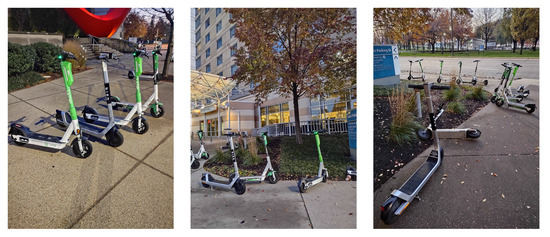
Figure 5.
Sample images from E-scooter dataset.
5.1. Common Objects in Context (COCO)
The COCO dataset serves as a benchmark for various object detection and segmentation tasks [17,28,29,54]. It contains 80 categories of objects, with more than 122k images. The wide variety of objects in various surroundings presents a complicated challenge for the object detectors.
5.2. SKU-110K
The SKU110K dataset was released in 2019 and contains 11,762 images with densely packed objects [23]. The dataset was collected from supermarkets worldwide and has about 147 objects/images. The objects in this dataset are significantly smaller in size and densely packed. This dataset contains 600 classes and approximately 2.3 classes/images. The training dataset contains 8k images with 90k bounding boxes, and the validation dataset contains 2.9k images with 432k bounding boxes. SKU110k has an average of 147 objects/image compared to PASCAL, with 2.71 and COCO (2015) with 7.7 objects/image [55].
5.3. Custom Dataset
To further experiment and evaluate our results, we prepared a custom dataset in two phases; in the first phase, e-scooter images were web-scrapped from the internet. The second phase of data collection was carried out due to the limited number of diverse images available online. In this phase, e-scooter images were captured manually across different urban landscapes such as school zones, parking spaces, and street walks. The dataset comprises images with the target object, e-scooters in various orientations, and different daylight conditions. Data augmentation was carried out by applying Gaussian noise, rotation of images, and adjusting brightness or a combination of these methods to the collected images to increase the results’ robustness further. These data augmentation methods helped diversify the data during the training and evaluation phases.
Annotation plays an essential role in the dataset preparation stage. A simple and effective annotation tool widely used for object detector modules is LabelImg. LabelImg is a graphical image annotation tool written in Python that uses Qt for its graphical interface. The dataset was manually annotated using the LabelImg tool, which supports various formats. Annotation was performed on a single class to target e-scooters in the augmented images. The training and testing images were split in an 80:20 ratio from the total images in the dataset. In this research, all the input images were originally resized to 640 × 640 pixels before implementing annotation for detecting e-scooters.
6. Experimental Setup
To evaluate the performance of the proposed BIoU loss and to compare the performance with various other losses, a simulation experiment was carried out first, followed by an implementation of loss function in the YOLOv5 and Mask_RCNN [54] object detectors.
6.1. Ablation Study
To completely understand and evaluate the performance of the loss functions, we first carried out a simulation experiment with synthetic data, similar to [31]. This step is crucial to understanding how the bounding box regression occurs in dynamic cases where prediction and ground truth boxes are of different sizes, aspect ratios, or scales. This experiment helped to analyze and understand the performance of different loss functions under the same control variables.
- The center coordinates of the ground truth box were fixed at (10, 10). The width-to-height ratio was kept at one, and various aspect ratios were considered, such as 1:4, 1:3, 1:2, 1:1, 2:1, 3:1, and 4:1.
- Five thousand data points of uniformly distributed anchor boxes were chosen with seven aspect ratios and scales. The anchor boxes also had a similar range of aspect ratios compared to ground truths and various areas, such as 0.5, 0.67, 0.75, 1, 1.33, 1.5, and 2.
- A total of 1,715,000 (7 aspect ratios × 7 different scales × 7 different areas × 5000 data points) regression cases and 200 iterations were carried out in the simulation experiment.
Bounding box regression was calculated at each step using the gradient descent algorithm as below:
where denotes the gradient loss at iteration (). To aid in the convergence, was utilized a multiplication factor. -norm was utilized to calculate the regression error, and gradient descent was utilized to optimize the algorithm.
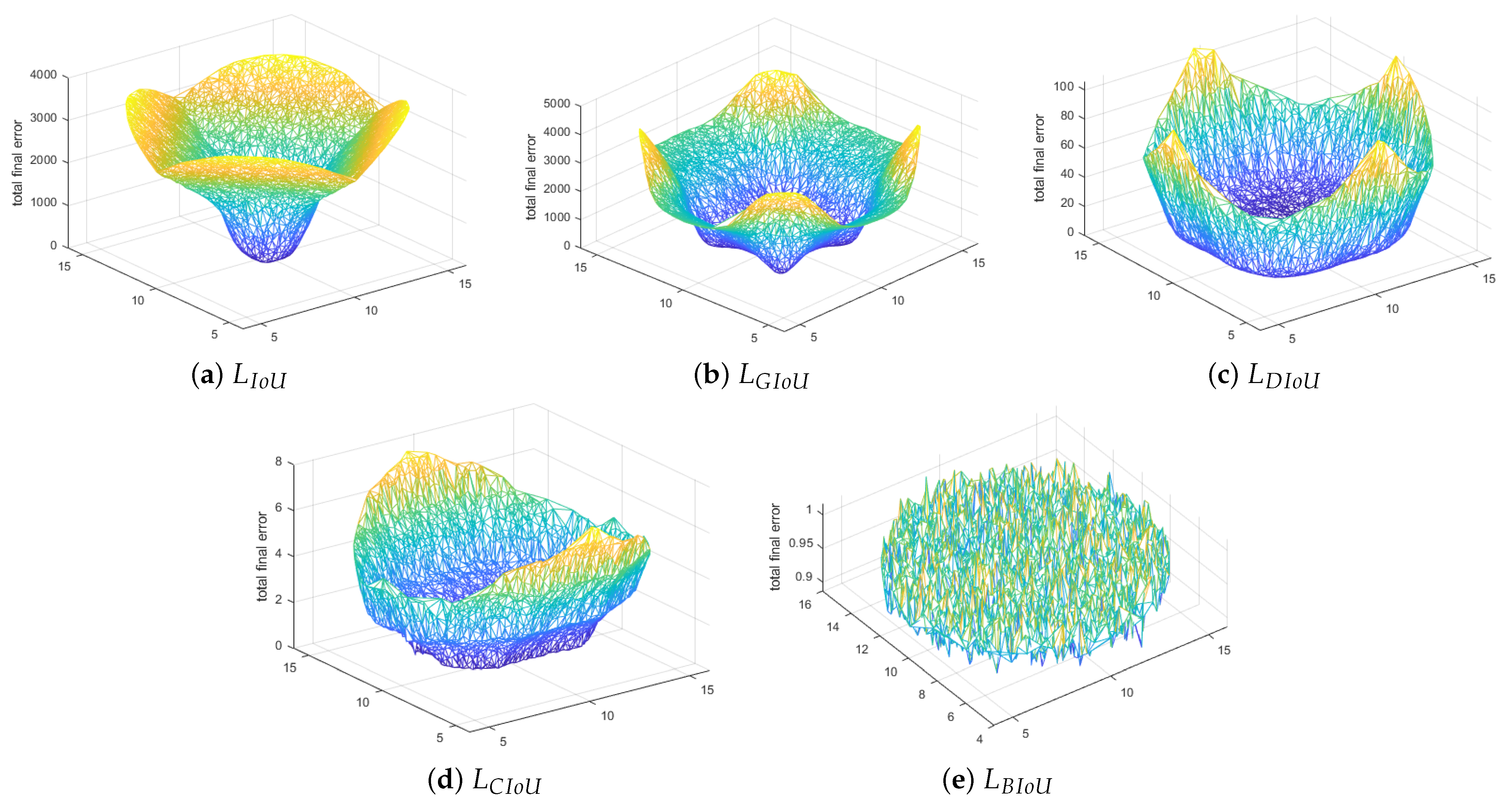
From Figure 6a, we can observe that IoU loss optimizes well near the initial point (10, 10) and the cases where bounding boxes overlap. The regression curve of GIoU loss is slightly better than IoU, shown in Figure 6b, but suffers many errors in horizontal and vertical cases. From Figure 6c,d, we can observe that DIoU and CIoU can optimize the initial bounding boxes but perform poorly towards the edge of the basin. This could be due to cases of inclusion, where one box is inside another with the same aspect ratios or centers. On the other hand, the proposed BIoU has much fewer regression errors throughout the distribution of data points and at any given random point, as seen in Figure 6e. The cumulative regression error at the end of 200 iterations was observed as follows: IoU had a total regression error of , whereas GIoU, DIoU, and CIoU were , , and . The newly proposed BIoU loss had the least cumulative regression error, .
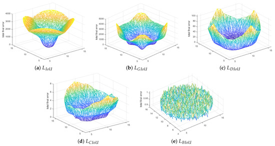
Figure 6.
Illustration of various regression curves of IoU, GIoU, DIoU, CIoU, and BIoU at the 200th iteration in three dimensions.
6.2. Evaluation on Object Detectors
The performance of the proposed BIoU loss was investigated on both two-stage object detectors (Mask_RCNN) [56] and a single-stage detector (YOLOv5). Resnet 101 was chosen as a backbone for Mask_RCNN. YOLOv5 is one of the latest advancements in single-stage object detection due to its tiny network structure and higher performance in benchmark datasets [22,53,57]. The network structure utilized CSPDarknet as a backbone, which aids in building feature maps. Fewer network parameters also increase the network’s overall performance in real-time detection [58]. To provide a fair comparison between different loss functions, hyper-parameters and other factors were kept constant during the network training phase. Carbonate, an initiative by Indiana University to provide a computer cluster equipped with Intel Xeon Gold 6126 12-core CPUs and Tesla V100 GPUs, was utilized for training and evaluating the performance. Mask_RCNN was trained and evaluated on the COCO dataset with a batch size of 2 and image size of 1024 × 1024. The YOLOv5n6 network with 3.2 million parameters was used to train and assess the SKU110k dataset, whereas YOLOv5x with 86.7 million parameters was chosen to train and evaluate the custom e-scooter dataset. The YOLOv5 networks were trained with a batch size of 128 and image size of 512 × 512. All the loss functions were evaluated using the IoU metric, and their respective results are tabulated in terms of various levels of average precision (AP), such as AP50 to AP95. AP50 indicates 50% overlap, and AP95 indicates 95% overlap between the predicted and ground truth bounding boxes. AP50:95 indicates an average of overlaps between 50 and 95%. , , indicate average precision for small, medium and large objects in the test dataset. Separate evaluation scripts were executed for IoU, GIoU, DIoU, CIoU, and BIoU losses, and results are tabulated in Table 1, Table 2 and Table 3. Absolute improvement is denoted as A.I, and relative improvement (R.L) in percentage is calculated for each loss.

Table 1.
Experimental evaluation of MASK_RCNN trained using , , , and . The results are reported on COCO dataset.

Table 2.
Experimental evaluation of YOLOv5n6 trained using , , , and . The results are reported on SKU 110 K.

Table 3.
Experimental evaluation of YOLOv5x trained using , , , and . The results are reported on e-scooter.
7. Performance Evaluation
In Table 1, the proposed performs remarkably well for AP 50:95 and AP_S, with gain values of 2.10% and 3.70% as compared to . From Table 2, we can see that gains peak performance at AP50 with 79.4%, and the gains gradually reduce as the overlap ratio increases. The losses , , do not perform well and have significantly lower AP gains compared to in the majority of the cases. This behavior could be because the number of objects in an image in the SKU110k dataset is very high and the smaller objects are densely packed in closer proximity. This creates more inclusion cases where bounding boxes of ground truth and prediction boxes partially or completely overlap with each other. Since , , and suffer drawbacks in the cases of inclusion, the overall performance of the network is reduced. On the other hand, the proposed has attained a peak performance at AP50 with 79.4% with a relative improvement of 5.86%. In particular, has a significant improvement in RL of 6.20% at AP55. We could observe a consistent increase in gains across all APs when compared with other losses.
Table 3 shows gains of 89.8% at AP50 and 72.9% at AP75. With as the benchmark, increases the accuracy by 1.33% at AP50 and 7.96% at AP70. However, performs poorly as compared to and at these APs. also performs slightly better than by 1.22% and 3.84%, but they are still lesser than the performance of at these AP values. shows a peak performance at AP50 with an increase of 2.22% compared to and improved detection accuracies from AP70 to AP95. By comparing between Table 1, Table 2 and Table 3, we could visualize the increase in performance with proposed ranges between 1.09% to 9.03%, wherein , , demonstrated the highest increments of 5.38%, 5.10%, and 5.20%. The reason for this phenomenon is because the proposed loss function considers additional edge cases where centers are aligned and the aspect ratio is equal. The number of such edge cases vastly depend on the type of dataset, number of objects and location of the objects in an image.
Additional Observations
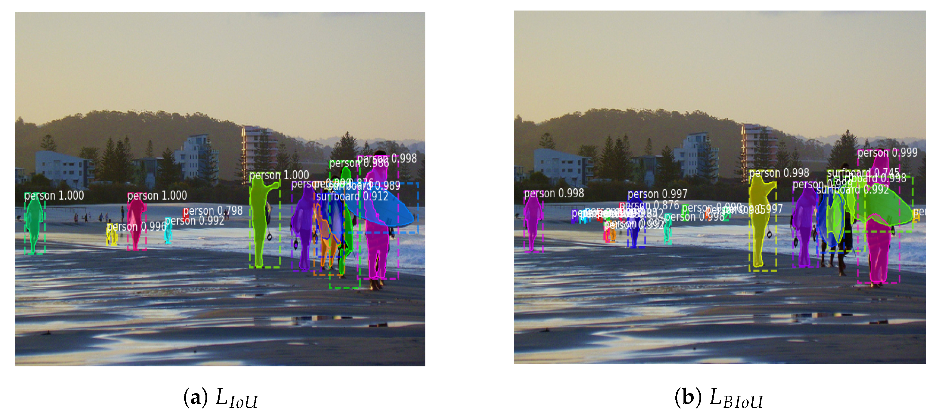
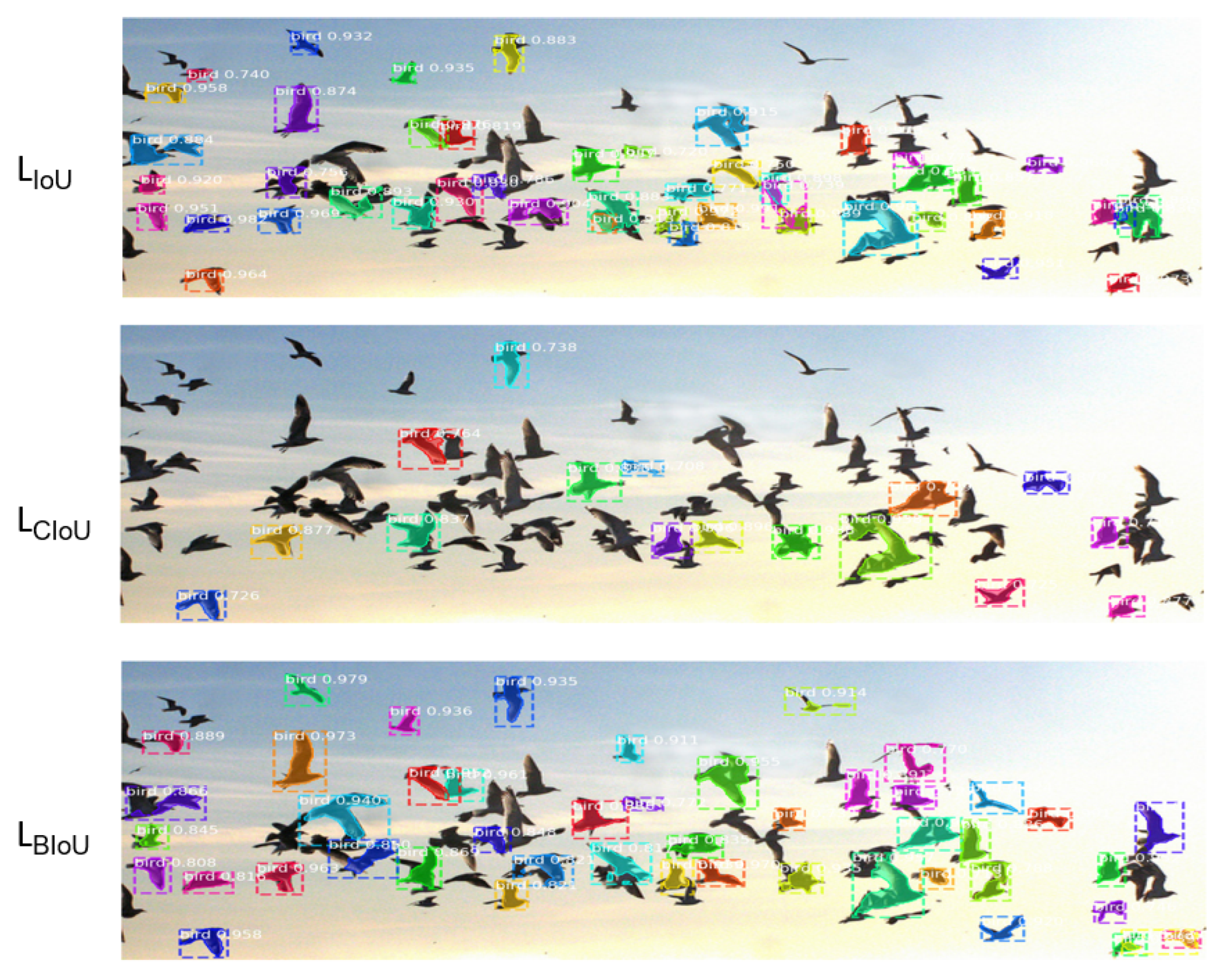
The space complexity of is O(1), so the loss function does not incur additional computational resources. We also compared the proposed with various loss functions such as scale-sensitive IoU (SIoU) and scale-balance IoU, and their performance was evaluated. On the SKU 110 K dataset, SIoU attained values of 74.4%, 70.4%, and 65.6% for AP50, AP55, and AP60, as compared to precision values of 79.40%, 75.30%, and 70.10%. demonstrates a 5% increase in precision values compared to SIoU. On the MS COCO dataset, when using the YOLOv3 network, scale-balance IoU achieves a 58.27% accuracy at AP50, where the proposed was able to attain 61.7%, demonstrating a 2.94% improvement. The trained model weights of , and from Mask_RCNN network were individually evaluated on test images of the COCO dataset and are displayed in Figure 7 and Figure 8. As we can visualize from Figure 7, the network with the proposed loss function could detect even smaller objects that are very far and closely located with each other. The number of objects detected with is significantly higher than . Figure 8 displays a similar behavior where has successfully detected more objects with higher confidence as compared to and .

Figure 7.
Detection results from MS COCO using Mask_RCNN trained using and .
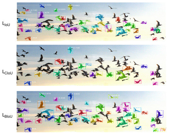
Figure 8.
Detection results from MS COCO using Mask_RCNN trained using , and .
8. Conclusions
In this research article, the drawbacks of existing IoU-based losses were studied, and a new loss function, , which considers the parameterized distance between the centers and the minimum and maximum edges to address the bounding box regression problem, was proposed. The efficiency of the network across various geometric factors such as aspect ratio, area, and scale were studied with the help of a simulation experiment. Experiments on COCO, SKU110K and the e-scooter dataset displayed state-of-art performance, and was able to improve the localization accuracy of the MASK_RCNN, YOLOv5n6 and YOLOv5x models. The future scope of this research involves the usage of LiDAR and camera sensors together to develop an efficient 3D object detection and tracking system to monitor e-scooter traffic. This system is to be installed in high-traffic areas to regulate e-scooter traffic and ensure the safety of pedestrians.
Author Contributions
Conceptualization, N.R., S.N., and M.E.-S.; methodology, N.R.; software, N.R and S.N..; validation, S.N. and M.E.-S.; writing—original draft preparation, N.R.; writing—review and editing, S.N. and and M.E.-S.; supervision, M.E.-S. All authors have read and agreed to the published version of the manuscript.
Funding
This research received no external funding.
Data Availability Statement
The data presented in this study are available on request from the corresponding author. The data are not publicly available due to the fact that all the authors work at the same institution and there is no necessity to create repository for data exchange.
Conflicts of Interest
The authors declare no conflict of interest.
References
- Anonymous. The Automobile: Effects/Impact on Society and Changes in Cars Made by Generation—AxleAddict. 2022. Available online: https://axleaddict.com/auto-industry/Affects-of-the-Automobile-on-Society-and-Changes-Made-by-Generation (accessed on 25 July 2022).
- Chitanvis, R.; Ravi, N.; Zantye, T.; El-Sharkawy, M. Collision avoidance and Drone surveillance using Thread protocol in V2V and V2I communications. In Proceedings of the 2019 IEEE National Aerospace and Electronics Conference (NAECON), Dayton, OH, USA, 15–19 July 2019; pp. 406–411. [Google Scholar]
- Katare, D.; El-Sharkawy, M. Embedded System Enabled Vehicle Collision Detection: An ANN Classifier. In Proceedings of the 2019 IEEE 9th Annual Computing and Communication Workshop and Conference (CCWC), Las Vegas, NV, USA, 7–9 January 2019; pp. 0284–0289. [Google Scholar] [CrossRef]
- Bergek, A.; Berggren, C.; KITE Research Group. The impact of environmental policy instruments on innovation: A review of energy and automotive industry studies. Ecol. Econ. 2014, 106, 112–123. [Google Scholar] [CrossRef]
- Electric Scooters Market Size, Share & Trends Analysis Report by Product (Retro, Standing/Self-Balancing, Folding), by Battery (Sealed Lead Acid, NiMH, Li-Ion), by Voltage, and Segment Forecasts, 2022–2030. 2022. Available online: https://www.grandviewresearch.com/industry-analysis/electric-scooters-market (accessed on 25 July 2022).
- Kobayashi, L.M.; Williams, E.; Brown, C.V.; Emigh, B.J.; Bansal, V.; Badiee, J.; Checchi, K.D.; Castillo, E.M.; Doucet, J. The e-merging e-pidemic of e-scooters. Trauma Surg. Acute Care Open 2019, 4, e000337. [Google Scholar] [CrossRef] [PubMed]
- Gössling, S. Integrating e-scooters in urban transportation: Problems, policies, and the prospect of system change. Transp. Res. Part D Transp. Environ. 2020, 79, 102230. [Google Scholar] [CrossRef]
- Tuncer, S.; Brown, B. E-scooters on the ground: Lessons for redesigning urban micro-mobility. In Proceedings of the 2020 CHI Conference on Human Factors in Computing Systems, Honolulu, HI, USA, 25–30 April 2020; pp. 1–14. [Google Scholar]
- Venkitachalam, S.; Manghat, S.K.; Gaikwad, A.S.; Ravi, N.; Bhamidi, S.B.S.; El-Sharkawy, M. Realtime applications with rtmaps and bluebox 2.0. In Proceedings of the International Conference on Artificial Intelligence (ICAI), Las Vegas, NV, USA, 30 July–2 August 2018; pp. 137–140. [Google Scholar]
- Zou, Z.; Shi, Z.; Guo, Y.; Ye, J. Object detection in 20 years: A survey. arXiv 2019, arXiv:1905.05055. [Google Scholar]
- Girshick, R.; Donahue, J.; Darrell, T.; Malik, J. Rich feature hierarchies for accurate object detection and semantic segmentation. In Proceedings of the IEEE Conference on Computer Vision and Pattern Recognition, Columbus, OH, USA, 23–28 June 2014; pp. 580–587. [Google Scholar]
- Katare, D.; El-Sharkawy, M. Real-Time 3-D Segmentation on An Autonomous Embedded System: Using Point Cloud and Camera. In Proceedings of the 2019 IEEE National Aerospace and Electronics Conference (NAECON), Dayton, OH, USA, 15–19 July 2019; pp. 356–361. [Google Scholar] [CrossRef]
- Redmon, J.; Farhadi, A. Yolov3: An incremental improvement. arXiv 2018, arXiv:1804.02767. [Google Scholar]
- Redmon, J.; Divvala, S.; Girshick, R.; Farhadi, A. You only look once: Unified, real-time object detection. In Proceedings of the IEEE Conference on Computer Vision and Pattern Recognition, Las Vegas, NV, USA, 27–30 June 2016; pp. 779–788. [Google Scholar]
- Ieamsaard, J.; Charoensook, S.N.; Yammen, S. Deep learning-based face mask detection using yoloV5. In Proceedings of the 2021 9th International Electrical Engineering Congress (iEECON), Pattaya, Thailand, 10–12 March 2021; pp. 428–431. [Google Scholar]
- Liu, W.; Anguelov, D.; Erhan, D.; Szegedy, C.; Reed, S.; Fu, C.Y.; Berg, A.C. Ssd: Single shot multibox detector. In Proceedings of the European Conference on Computer Vision, Amsterdam, The Netherlands, 11–14 October 2016; pp. 21–37. [Google Scholar]
- Ren, S.; He, K.; Girshick, R.; Sun, J. Faster r-cnn: Towards real-time object detection with region proposal networks. Adv. Neural Inf. Process. Syst. 2015, 28, 1–14. [Google Scholar] [CrossRef]
- Wang, Q.; Cheng, J. LCornerIoU: An Improved IoU-based Loss Function for Accurate Bounding Box Regression. In Proceedings of the 2021 International Conference on Intelligent Computing, Automation and Systems (ICICAS), Chongqing, China, 29–31 December 2021; pp. 377–383. [Google Scholar]
- Sun, D.; Yang, Y.; Li, M.; Yang, J.; Meng, B.; Bai, R.; Li, L.; Ren, J. A scale balanced loss for bounding box regression. IEEE Access 2020, 8, 108438–108448. [Google Scholar] [CrossRef]
- Zheng, Z.; Wang, P.; Ren, D.; Liu, W.; Ye, R.; Hu, Q.; Zuo, W. Enhancing geometric factors in model learning and inference for object detection and instance segmentation. IEEE Trans. Cybern. 2022, 52, 8574–8586. [Google Scholar] [CrossRef]
- Wang, Y.; Zhao, X.; Hu, X.; Li, Y.; Huang, K. Focal boundary guided salient object detection. IEEE Trans. Image Process. 2019, 28, 2813–2824. [Google Scholar] [CrossRef]
- Lin, T.Y.; Maire, M.; Belongie, S.; Hays, J.; Perona, P.; Ramanan, D.; Dollár, P.; Zitnick, C.L. Microsoft coco: Common objects in context. In Proceedings of the European Conference on Computer Vision, Zurich, Switzerland, 6–12 September 2014; pp. 740–755. [Google Scholar]
- Goldman, E.; Herzig, R.; Eisenschtat, A.; Goldberger, J.; Hassner, T. Precise detection in densely packed scenes. In Proceedings of the IEEE/CVF Conference on Computer Vision and Pattern Recognition, Long Beach, CA, USA, 15–20 June 2019; pp. 5227–5236. [Google Scholar]
- Vidhya, C.B.A. Evolution of Object Detection. 2020. Available online: https://medium.com/analytics-vidhya/evolution-of-object-detection-582259d2aa9b (accessed on 25 July 2022).
- Dalal, N.; Triggs, B. Histograms of oriented gradients for human detection. In Proceedings of the 2005 IEEE Computer Society Conference on Computer Vision and Pattern Recognition (CVPR’05), San Diego, CA, USA, 20–26 June 2005; Volume 1, pp. 886–893. [Google Scholar] [CrossRef]
- Girshick, R.; Iandola, F.; Darrell, T.; Malik, J. Deformable part models are convolutional neural networks. In Proceedings of the IEEE Conference on Computer Vision and Pattern Recognition, Boston, MA, USA, 7–12 June 2015; pp. 437–446. [Google Scholar]
- Mallick, S. Histogram of Oriented Gradients Explained Using OpenCV. 2016. Available online: https://learnopencv.com/histogram-of-oriented-gradients/ (accessed on 26 July 2022).
- Girshick, R. Fast r-cnn. In Proceedings of the IEEE International Conference on Computer Vision, Santiago, Chile, 7–13 December 2015; pp. 1440–1448. [Google Scholar]
- Dwivedi, P. YOLOv5 Compared to Faster RCNN. Who Wins? 2020. Available online: https://towardsdatascience.com/yolov5-compared-to-faster-rcnn-who-wins-a771cd6c9fb4 (accessed on 27 July 2022).
- Redmon, J.; Farhadi, A. YOLO9000: Better, faster, stronger. In Proceedings of the IEEE Conference on Computer Vision and Pattern Recognition, Honolulu, HI, USA, 21–26 July 2017; pp. 7263–7271. [Google Scholar]
- Zheng, Z.; Wang, P.; Liu, W.; Li, J.; Ye, R.; Ren, D. Distance-IoU loss: Faster and better learning for bounding box regression. In Proceedings of the AAAI Conference on Artificial Intelligence, New York, NY, USA, 7–8 February 2020; Volume 34, pp. 12993–13000. [Google Scholar]
- Wang, G.; Zhuang, Y.; Chen, H.; Liu, X.; Zhang, T.; Li, L.; Dong, S.; Sang, Q. FSoD-Net: Full-scale object detection from optical remote sensing imagery. IEEE Trans. Geosci. Remote Sens. 2021, 60, 1–18. [Google Scholar] [CrossRef]
- Cheng, G.; Si, Y.; Hong, H.; Yao, X.; Guo, L. Cross-scale feature fusion for object detection in optical remote sensing images. IEEE Geosci. Remote Sens. Lett. 2020, 18, 431–435. [Google Scholar] [CrossRef]
- Deng, Z.; Sun, H.; Zhou, S.; Zhao, J.; Lei, L.; Zou, H. Multi-scale object detection in remote sensing imagery with convolutional neural networks. ISPRS J. Photogramm. Remote Sens. 2018, 145, 3–22. [Google Scholar] [CrossRef]
- Bao, S.; Zhong, X.; Zhu, R.; Zhang, X.; Li, Z.; Li, M. Single shot anchor refinement network for oriented object detection in optical remote sensing imagery. IEEE Access 2019, 7, 87150–87161. [Google Scholar] [CrossRef]
- Xu, Z.; Xu, X.; Wang, L.; Yang, R.; Pu, F. Deformable convnet with aspect ratio constrained nms for object detection in remote sensing imagery. Remote Sens. 2017, 9, 1312. [Google Scholar] [CrossRef]
- Hong, D.; Gao, L.; Yao, J.; Zhang, B.; Plaza, A.; Chanussot, J. Graph convolutional networks for hyperspectral image classification. IEEE Trans. Geosci. Remote Sens. 2020, 59, 5966–5978. [Google Scholar] [CrossRef]
- Wu, X.; Hong, D.; Tian, J.; Chanussot, J.; Li, W.; Tao, R. ORSIm detector: A novel object detection framework in optical remote sensing imagery using spatial-frequency channel features. IEEE Trans. Geosci. Remote Sens. 2019, 57, 5146–5158. [Google Scholar] [CrossRef]
- Hong, D.; Gao, L.; Yokoya, N.; Yao, J.; Chanussot, J.; Du, Q.; Zhang, B. More diverse means better: Multimodal deep learning meets remote-sensing imagery classification. IEEE Trans. Geosci. Remote Sens. 2020, 59, 4340–4354. [Google Scholar] [CrossRef]
- Hong, D.; Yokoya, N.; Chanussot, J.; Zhu, X.X. An augmented linear mixing model to address spectral variability for hyperspectral unmixing. IEEE Trans. Image Process. 2018, 28, 1923–1938. [Google Scholar] [CrossRef]
- Hang, R.; Li, Z.; Ghamisi, P.; Hong, D.; Xia, G.; Liu, Q. Classification of hyperspectral and LiDAR data using coupled CNNs. IEEE Trans. Geosci. Remote Sens. 2020, 58, 4939–4950. [Google Scholar] [CrossRef]
- Yu, J.; Jiang, Y.; Wang, Z.; Cao, Z.; Huang, T. Unitbox: An advanced object detection network. In Proceedings of the 24th ACM International Conference on Multimedia, Amsterdam, The Netherlands, 15–19 October 2016; pp. 516–520. [Google Scholar]
- Rezatofighi, H.; Tsoi, N.; Gwak, J.; Sadeghian, A.; Reid, I.; Savarese, S. Generalized intersection over union: A metric and a loss for bounding box regression. In Proceedings of the IEEE/CVF Conference on Computer Vision and Pattern Recognition, Long Beach, CA, USA, 15–20 June 2019; pp. 658–666. [Google Scholar]
- Zhang, Y.F.; Ren, W.; Zhang, Z.; Jia, Z.; Wang, L.; Tan, T. Focal and efficient IOU loss for accurate bounding box regression. arXiv 2021, arXiv:2101.08158. [Google Scholar] [CrossRef]
- Wang, X.; Song, J. ICIoU: Improved loss based on complete intersection over union for bounding box regression. IEEE Access 2021, 9, 105686–105695. [Google Scholar] [CrossRef]
- Du, S.; Zhang, B.; Zhang, P.; Xiang, P. An Improved Bounding Box Regression Loss Function Based on CIOU Loss for Multi-scale Object Detection. In Proceedings of the 2021 IEEE 2nd International Conference on Pattern Recognition and Machine Learning (PRML), Chengdu, China, 16–18 July 2021; pp. 92–98. [Google Scholar]
- Du, S.; Zhang, B.; Zhang, P. Scale-Sensitive IOU Loss: An Improved Regression Loss Function in Remote Sensing Object Detection. IEEE Access 2021, 9, 141258–141272. [Google Scholar] [CrossRef]
- Wu, S.; Yang, J.; Wang, X.; Li, X. Iou-balanced loss functions for single-stage object detection. Pattern Recognit. Lett. 2022, 156, 96–103. [Google Scholar] [CrossRef]
- Zhang, H.; Wang, Y.; Dayoub, F.; Sunderhauf, N. Varifocalnet: An iou-aware dense object detector. In Proceedings of the IEEE/CVF Conference on Computer Vision and Pattern Recognition, Nashville, TN, USA, 19–25 June 2021; pp. 8514–8523. [Google Scholar]
- Chen, Z.; Chen, K.; Lin, W.; See, J.; Yu, H.; Ke, Y.; Yang, C. Piou loss: Towards accurate oriented object detection in complex environments. In Proceedings of the European Conference on Computer Vision, Glasgow, UK, 23–28 August 2020; pp. 195–211. [Google Scholar]
- Zhou, D.; Fang, J.; Song, X.; Guan, C.; Yin, J.; Dai, Y.; Yang, R. Iou loss for 2d/3d object detection. In Proceedings of the 2019 International Conference on 3D Vision (3DV), Quebec City, QC, Canada, 16–19 September 2019; pp. 85–94. [Google Scholar]
- Yang, X.; Yan, J.; Ming, Q.; Wang, W.; Zhang, X.; Tian, Q. Rethinking rotated object detection with gaussian wasserstein distance loss. In Proceedings of the International Conference on Machine Learning, Virtual, 18–24 July 2021; pp. 11830–11841. [Google Scholar]
- Ravi, N.; El-Sharkawy, M. Real-Time Embedded Implementation of Improved Object Detector for Resource-Constrained Devices. J. Low Power Electron. Appl. 2022, 12, 21. [Google Scholar] [CrossRef]
- He, K.; Gkioxari, G.; Dollár, P.; Girshick, R. Mask r-cnn. In Proceedings of the IEEE International Conference on Computer Vision, Venice, Italy, 22–29 October 2017; pp. 2961–2969. [Google Scholar]
- Hu, D. An introductory survey on attention mechanisms in NLP problems. In Proceedings of the SAI Intelligent Systems Conference, London, UK, 5–6 September 2019; pp. 432–448. [Google Scholar]
- Abdulla, W. Mask R-CNN for Object Detection and Instance Segmentation on Keras and TensorFlow. 2017. Available online: https://github.com/matterport/Mask_RCNN (accessed on 20 July 2022).
- Everingham, M.; Van Gool, L.; Williams, C.K.; Winn, J.; Zisserman, A. The pascal visual object classes (voc) challenge. Int. J. Comput. Vis. 2010, 88, 303–338. [Google Scholar] [CrossRef]
- Kalgaonkar, P.; El-Sharkawy, M. Condensenext: An ultra-efficient deep neural network for embedded systems. In Proceedings of the 2021 IEEE 11th Annual Computing and Communication Workshop and Conference (CCWC), Las Vegas, NV, USA, 27–30 January 2021; pp. 0524–0528. [Google Scholar]
Publisher’s Note: MDPI stays neutral with regard to jurisdictional claims in published maps and institutional affiliations. |
© 2022 by the authors. Licensee MDPI, Basel, Switzerland. This article is an open access article distributed under the terms and conditions of the Creative Commons Attribution (CC BY) license (https://creativecommons.org/licenses/by/4.0/).

