Mathematical Modeling and Simulation of the COVID-19 Pandemic

Abstract

The current pandemic is a great challenge for several research areas. In addition to virology research, mathematical models and simulations can be a valuable contribution to the understanding of the dynamics of the pandemic and can give recommendations to physicians and politicians. Based on actual data of people infected with COVID-19 from the European Center for Disease Prevention and Control (ECDC), input parameters of mathematical models will be determined and applied. These parameters will be estimated for the UK, Italy, Spain, and Germany and used in an $SIR$-type model. As a basis for the model’s calibration, the initial exponential growth phase of the COVID-19 pandemic in the named countries is used. Strategies for the commencing and ending of social and economic shutdown measures are discussed.

1. Introduction

COVID-19 is a recent emerging disease caused by the emerging coronavirus. As there is no immunity to this virus, the spread of the disease has been rampant worldwide. As no serious vaccine or medication exists, it is necessary to look for effective non-pharmaceutical interventions to control the pandemic. Here, I use an $SIR$-type model to understand and analyze the COVID-19 pandemic with the aim of stopping or reducing the spread of the COVID-19 virus.

The dynamic development of sub-populations of susceptible (S), infected (I), and recovered (R) people in a certain region—for example, the population of a country or a part of a federation— depending on non-pharmaceutical interventions is the aim of the modeling. Deterministic models are discussed. These are simple but effective for describing the progression of the pandemic. They are able to fit the description of the average infection dynamics in macroscopic sub-populations only1.

The main scope of this paper is the investigation of certain lockdown measures to flatten the curve of infected people over time and of the appropriate strategies for returning from lockdown to normality. To find appropriate model parameters, real data of the early stages of the pandemic are analyzed. Suggestions about favorable points in time at which to commence with lockdown measures based on the acceleration rate of infections conclude the paper.

There are also more complex deterministic models, which include sub-populations other than S, I, and R (see [1,2]), but these models have dynamic properties similar to those of the basic $SIR$ model. On the other hand, additional data, which are not available, are needed for the extension of the basic model. This why I can perform the investigations on the basis of the $SIR$ model without a loss of generality with respect to the aim of this paper.

It is necessary to remark that the considered $SIR$ model is not able to describe the full asymptotic behavior of a pandemic, as is done in [3]. In addition, the role of super-spreaders, investigated in [4] and [5], cannot be described with the basic macroscopic $SIR$ model.

2. The Mathematical $SIR$ Model

First, I note one important presupposition for the model. I suppose that the distribution of the included sub-populations is equal, i.e., the density is approximately constant. This is a very strict supposition, but this is acceptable, for example, for cities and congested urban areas like New York or the Ruhr area in Germany. At the beginning of the pandemic, exponential growth of the number of infected people is supposed.

In the so-called $SIR$ model of Kermack and McKendrick [6], I denotes the infected people, S denotes the susceptible people, and R denotes the recovered people. It is a deterministic model. I constrain the investigations to the species I, S, and R only. The dynamics of infections and recoveries can be approximated by the following system of ordinary differential equations:

$$\begin{array}{ccc}\hfill \frac{dS}{dt}& =& -\kappa \beta \frac{S}{N}I\hfill \end{array}$$

(1)

$$\begin{array}{ccc}\hfill \frac{dI}{dt}& =& \kappa \beta \frac{S}{N}I-\gamma I\hfill \end{array}$$

(2)

$$\begin{array}{ccc}\hfill \frac{dR}{dt}& =& \gamma I.\hfill \end{array}$$

(3)

$\beta$ represents the number of others that one infected person encounters per unit time (per day). $\gamma$ is the reciprocal value of the typical time from infection to recovery. N is the total number of people involved in the epidemic disease, and $N=S+I+R$. $\kappa$ is equal to one in the case of an undisturbed pandemic without any interventions or lockdowns. Later, I will specify $\kappa$ as a function to describe lockdown measures.

The currently available empirical data suggest that the coronavirus infection typically lasts for some 14 days. This means that $\gamma =1/14\approx 0.7$.

The choice of $\beta$ is more complicated and will be considered in the following.

The equation system (1)–(3) belongs to the mathematical category of dynamical systems.

3. The Estimation of $\mathbf{\beta }$ Based on Real Data

I used the European Center for Disease Prevention and Control [7] to obtain data on the people infected with COVID-19 for the period from 31 January 2019 to 8 April 2020.

At the beginning of the pandemic, the quotient $S/N$ was nearly equal to 1. In addition, at the early stage, no one had yet recovered. Thus, I can describe the early regime using the ordinary differential equation

$$\frac{dI}{dt}=\beta I$$

with the solution

$$I\left(t\right)=I_{0}exp\left(\beta t\right).$$

(4)

The logarithm of (4) leads to

$$logI\left(t\right)=log{I}_0+\beta t.$$

Based on the table of logarithms of the infected people versus time, $(t_j,log{I}_j),j=1,\cdots ,k$, I look for $I_0$ and $\beta$ which minimize the function

$$L(I_0,\beta )=\sum _{j=1}^k{[log{I}_0+\beta t_j-log{I}_j]}^2.$$

(5)

The solution of this linear optimization problem is trivial, and it is available in most computer algebra systems as a ”black box” of the logarithmic–linear regression.

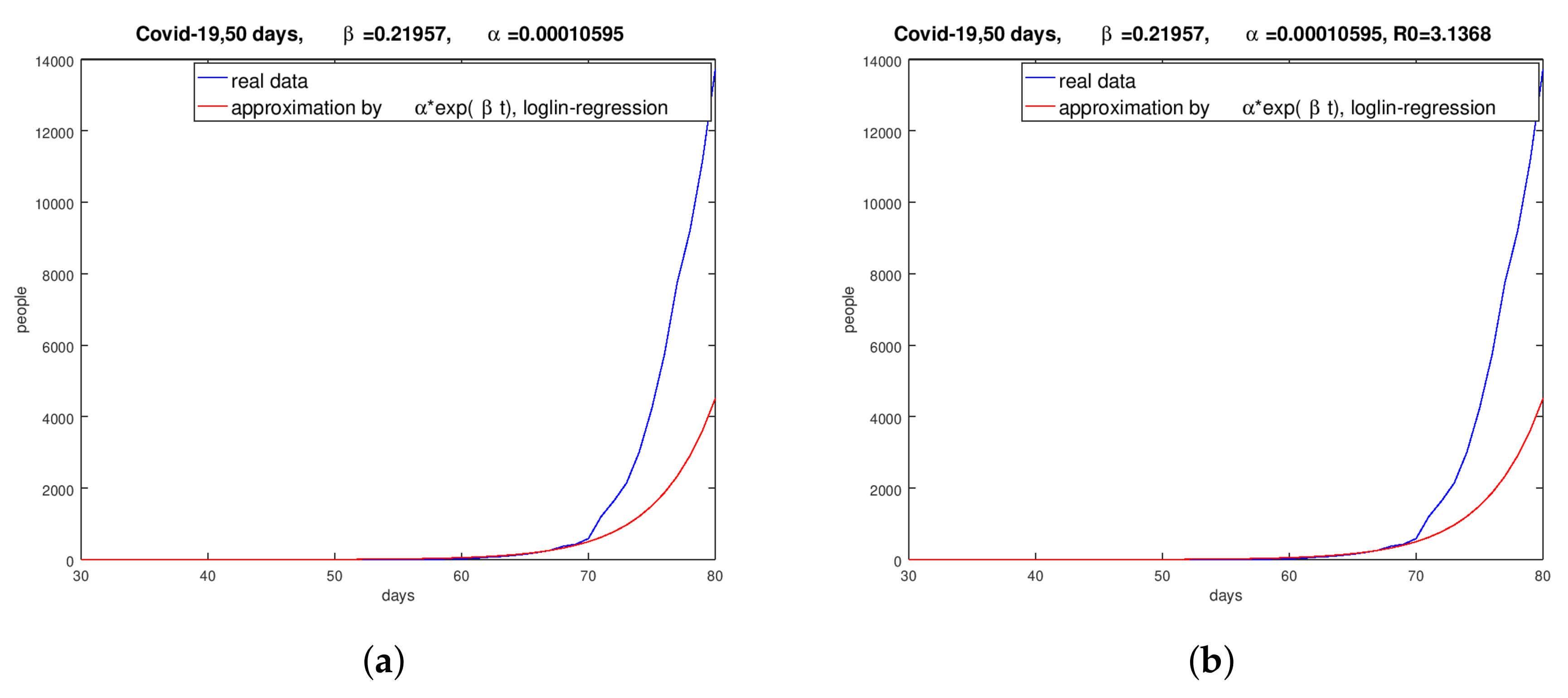
Figure 1 shows the results for the same periods as above for Spain and the UK2.

Figure 1 shows that the logarithmic–linear regression implies unsatisfactory results. It must be said that the evaluated $\beta$-values are related to the stated period. For the logarithmic–linear regression method, I guessed the respective periods for every country through a visual inspection of the graphs of the infected people versus time.

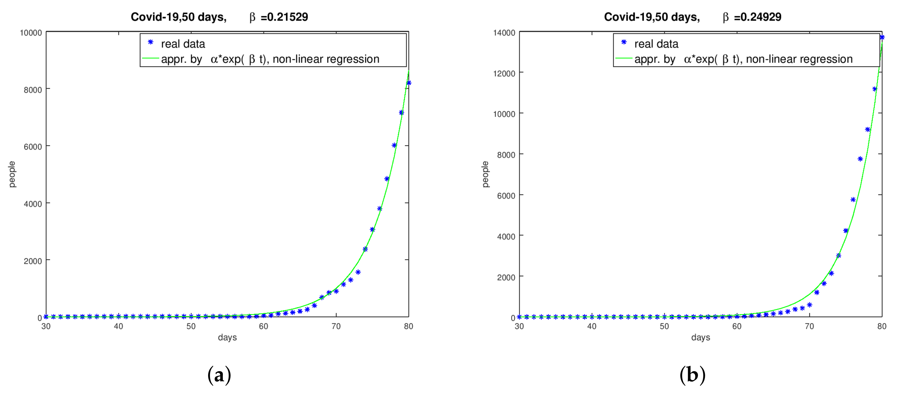
Instead of the above-used table of logarithmic values, the table $(t_j,I_j),j=1,\cdots ,k$ is used with the aim of a better approximation. I am looking for periods in the spreadsheets of infected people per day where the course can be described by a function of type (4).

Choosing a period $[t_1,t_k]$ for a certain country, I search for the minimum of the function

$$F(I_0,\beta )=\sum _{j=1}^k{[I_{0}exp\left(\beta t_j\right)-I_j]}^2,$$

i.e.,

$$\underset{(I_0,\beta )\in {\mathbb{R}}^2}{min}F(I_0,\beta ).$$

(6)

I solved this non-linear minimum problem with the damped Gauss–Newton method. The results of the above-discussed logarithmic–linear method for $\beta$ and $\alpha$ proved as good starting iterations for the Gauss–Newton method. I found the subsequent results for the considered countries. Thereby, I chose these periods for the countries with the aim of approximating the infection’s progression with a good quality. Figure 2 shows the graphs and the evaluated parameters for Germany and Spain.

I found some information on the parameters of Italy in [8]—for example, $\beta =0.25$—and I presume that this is a result of the logarithmic–linear regression by the Italian health administration.

A deeper look at the real data shows that the exponential behavior of the dynamic of the number of infected people was found only in the very beginning of the pandemic. In the German hotspot of Bavaria, I found the result $\beta =0.22658$ for the period from 24 February to 20 April 2020 with non-linear regression. With the logarithmic–linear approach, I found a quite similar value, $\beta =0.23$.

In conclusion, I can state that the estimation of the parameter $\beta$ is complicated but successful in most of the considered countries and regions. The results of the solution of the minimum problem (6) to evaluate $\beta$ are, in most cases, better than the results of the minimization of function (5) with respect to the fitting of the real data.

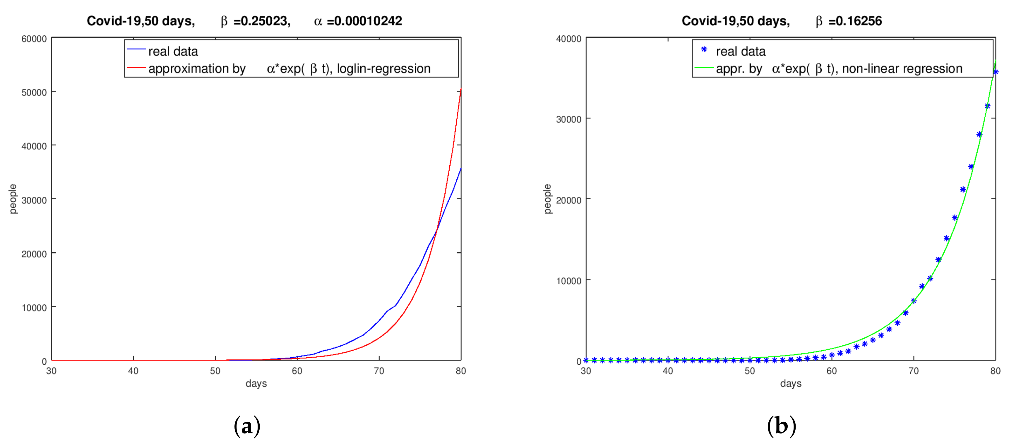
To illustrate the different quality and quantity of the $\beta$ estimation, I use Italy as an example in Figure 3.

4. Numerical Computations for Germany and Spain

I disclaim qualitative mathematical considerations like existence and uniqueness of solutions of the dynamical system of (1)–(3) and concentrate my interest on practical application and numerical experiments. The numerical solution of the ordinary differential equation system of the modified $SIR$ model was done with a Runge–Kutta integration method of the fourth order. The independence of the time discretization of the solution method was tested by a systematic time-grid refinement. At the end, I found that time-steps of half a day could be used. For all of the following computations, the $\beta$ results of the solution of the non-linear minimization problem are used.

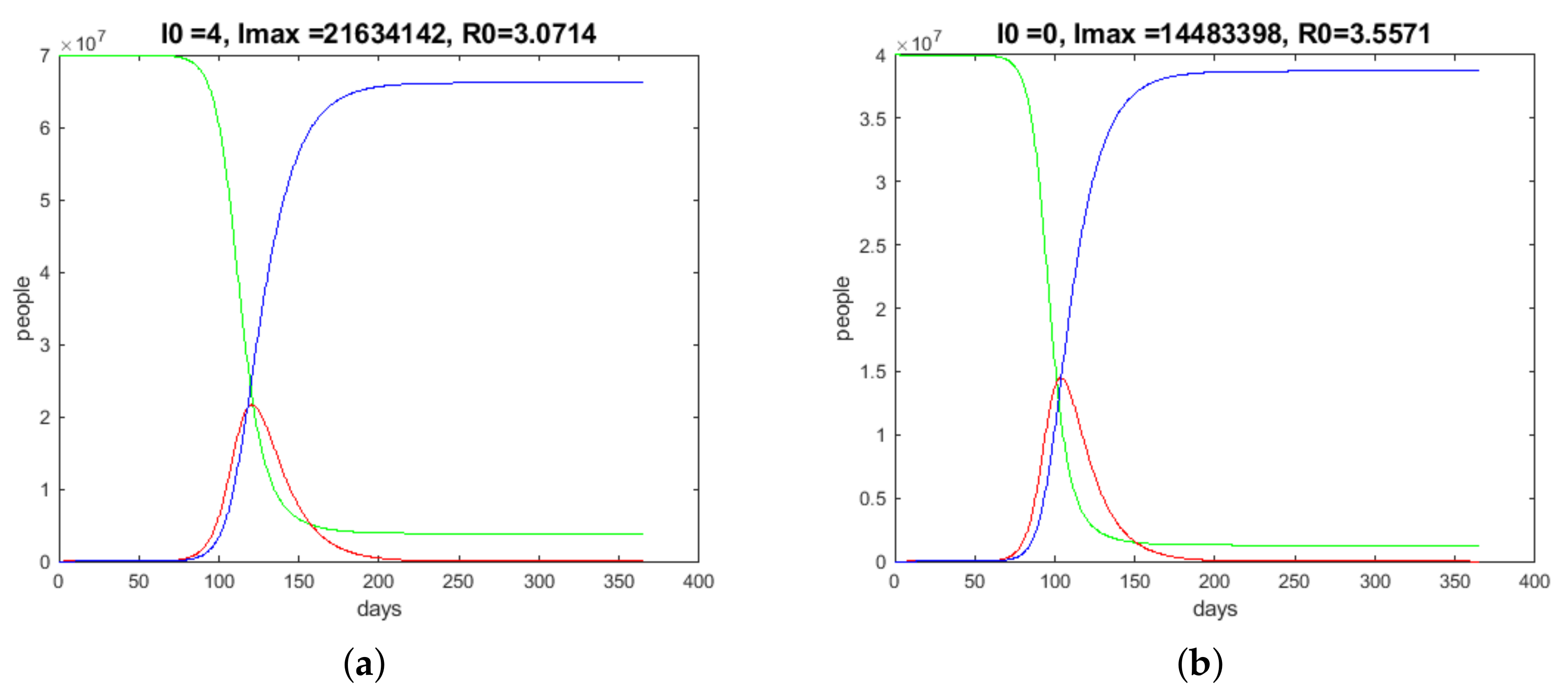
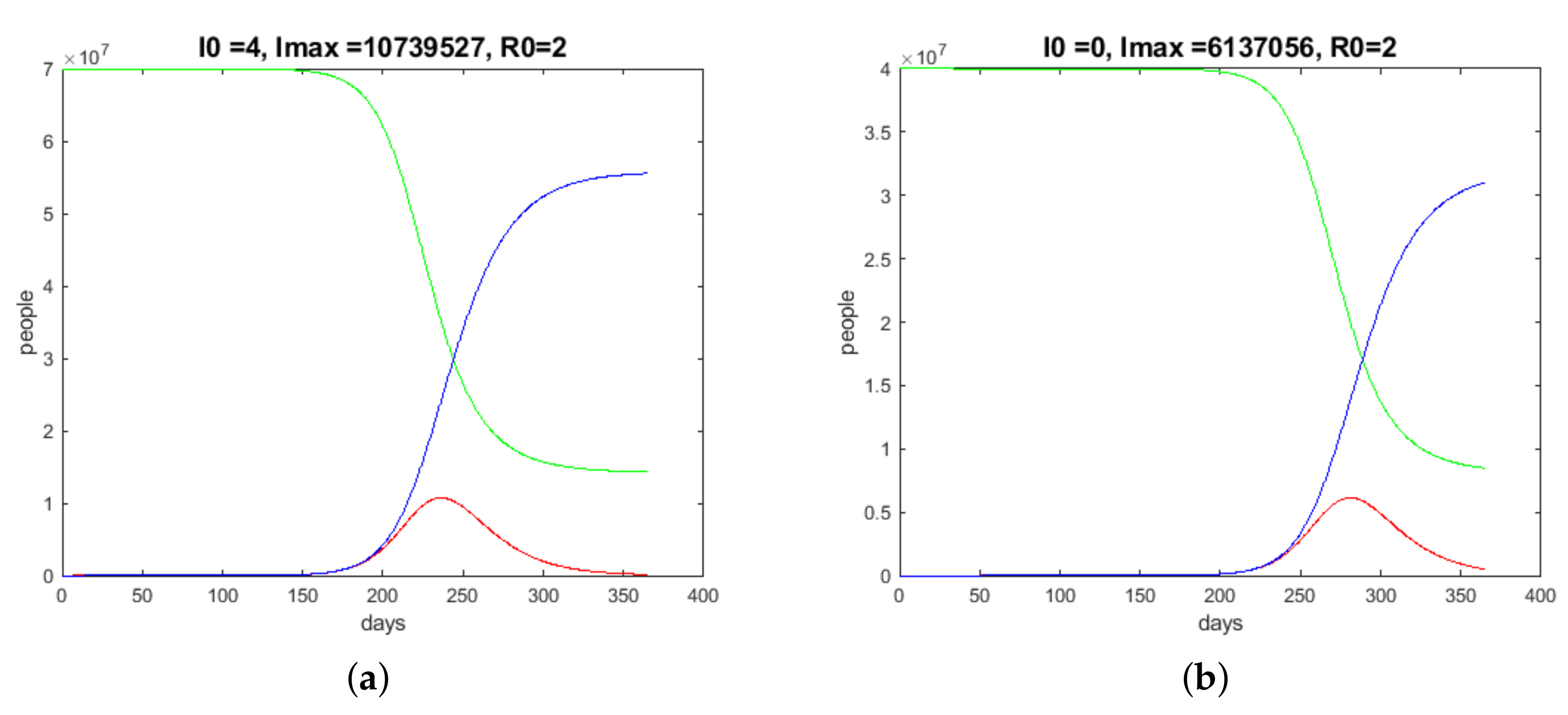
With the choice of a $\beta$-value of $0.215$ (see Figure 2a)—which is evaluated on the basis of the real data from the ECDC—and $\gamma =0.07$, one gets the progress of the pandemic’s dynamics, pictured in Figure 4a ($I0$ denotes the initial value of the I species, that is, 31 January 2020. $Imax$ stands for the maximum of I. The total number N for Germany is guessed to be 70 million). $R_0$ is the basis reproduction number of persons infected by the transmission of a pathogen from an infected person during the infectious time ($R_0=\beta /\gamma$), shown in the following figures3. For the early 30 days, I found a $\beta$-value of $0.36$ for China/Wuhan. This shows that the German situation with $\beta =0.215$ and $R_0\approx 3$ is moderate compared to the Chinese situation with the values $\beta \approx 0.36$ and $R_0\approx 5$. I have to mention that these values vary compared to those found by other authors, but the relationships between the German and the Chinese values are similar.

The data from the ECDC, the data from the German Robert Koch Institute, and the data from the Johns Hopkins University ([9]) are not really correct; thus, I have to reasonably assume that there are a number of unknown cases. It is guessed in [10] that the data cover only 15% of the real cases. Considering this, I obtained slightly changed results, and in the subsequent computations, I will include an estimated number of unknown cases in the initial values of I.

I use the $\beta$-value $0.249$ (see Figure 3) and $\gamma =0.07$ for Spain, and I get the run pictured in Figure 4. N is set to 40 million.

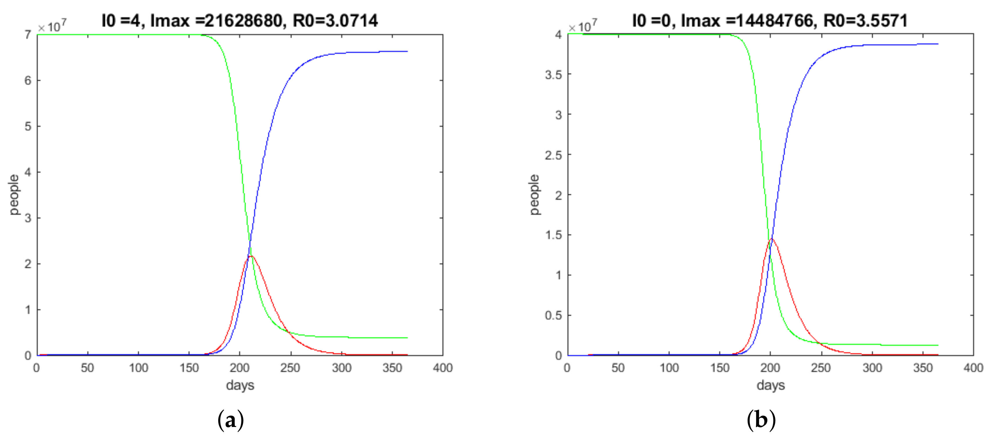
Let me now discuss the case of strict social distancing. To do this, I reduce the $\beta$-values after a few days to $\beta =0.14$ for both Germany and Spain.

The results in Figure 5 compared to the results without the reduction of $\beta$ (Figure 4) show the consequences. The climax of the number of infected people moved to the autumn of the year with hard inconveniences for the population, but the wanted flattening was achieved.

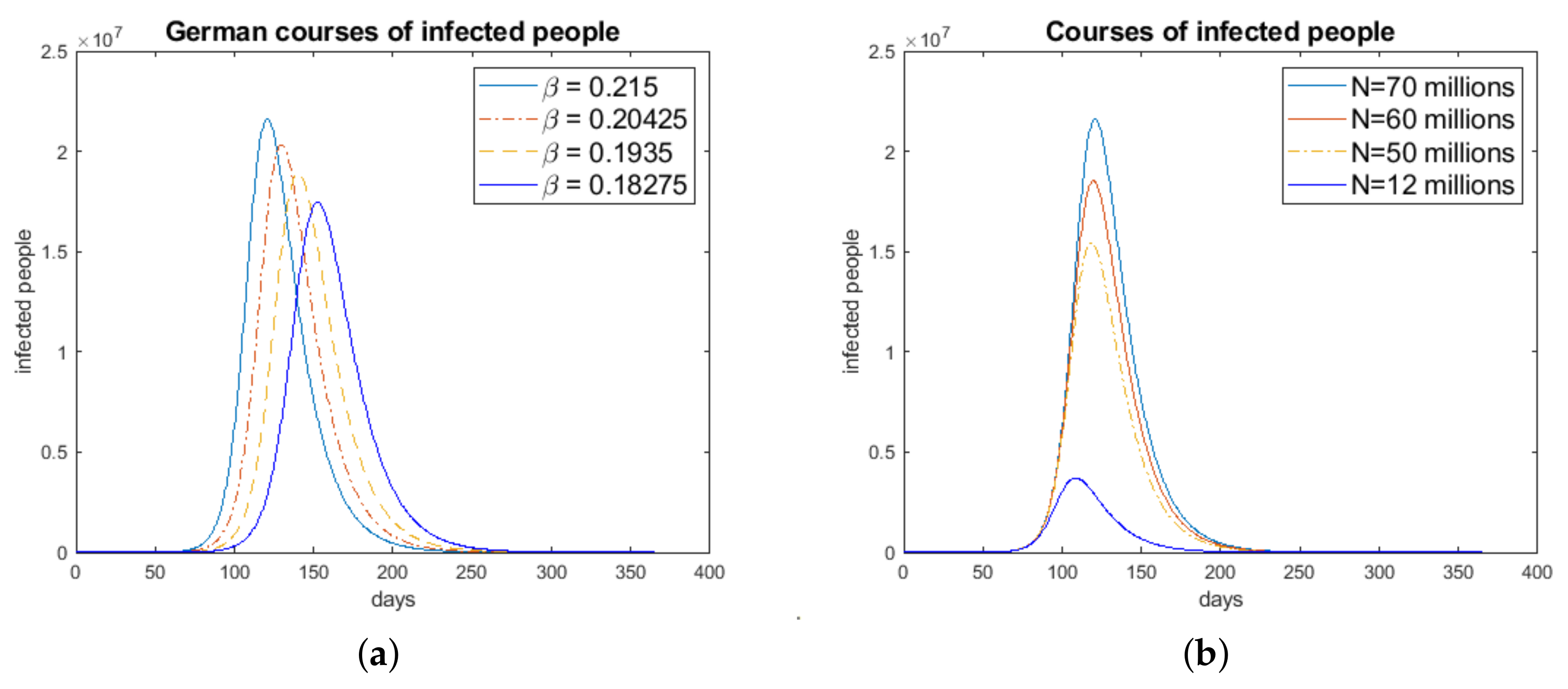
To investigate the influence and sensitivity of the simulation results with the parameter $\beta$ and the number N (sum of infected, susceptible, and recovered people), I used the German data and a variation of these data. In Figure 6b, I see that variation of the amount N leads, more or less, to a proportional scaling4. The variation of $\beta$ showed a non-monotone and non-linear influence of $\beta$ on the results, pictured in Figure 6a.

5. Looking for Other Strategies of a Temporary Lockdowns and Extensive Social Distancing

In all countries concerned by the COVID-19 pandemic, a lockdown of social life has been discussed. In Germany, the lockdown started on 16 March 2020. The effects of social distancing to decrease the infection rate can be modeled by a modification of the $SIR$ model. Now, I consider $\kappa$ in the equation system (1)–(3) as a time-dependent function (instead of $\kappa =1$ in the original $SIR$ model).

$\kappa$ is a function with values in $[0,1]$. For example,

$$\kappa \left(t\right)=\left\{\begin{array}{cc}0.5\hfill & \mathrm{for}{t}_0\le t\le t_1\hfill \\ 1\hfill & \mathrm{for}t>t_1,t<t_0\hfill \end{array}\right.$$

indicates a reduction of the infection rate of 50% in the period $[t_0,t_1]$ (${\Delta }_t=t_1-t_0$ is the duration of the temporary lockdown in days). A good choice of $t_0$ and $t_k$ will be complicated.

If I respect the chosen starting day of the German lockdown, 16th of March 2020 (this conforms to the 46th day of the relational year started at the end of January 2020), and I work5 with

$$\kappa \left(t\right)=\left\{\begin{array}{cc}0.2\hfill & \mathrm{for}46\le t\le 76\hfill \\ 1\hfill & \mathrm{for}t>76,t<46,\hfill \end{array}\right.$$

then I get the result pictured in Figure 7a.

The numerical tests showed that a very early start of the lockdown, resulting in a reduction of the infection rate $\beta$, causes the typical Gaussian curve to be delayed by I; however, the amplitude (maximum value of I) does not really change.

It is known from other pandemics, such as the Spanish flu ([11,12]) or the swine flu, that the development of the number of infected people looks like a Gaussian curve. The interesting points in time are those where the acceleration of the numbers of infected people increases or decreases, respectively.

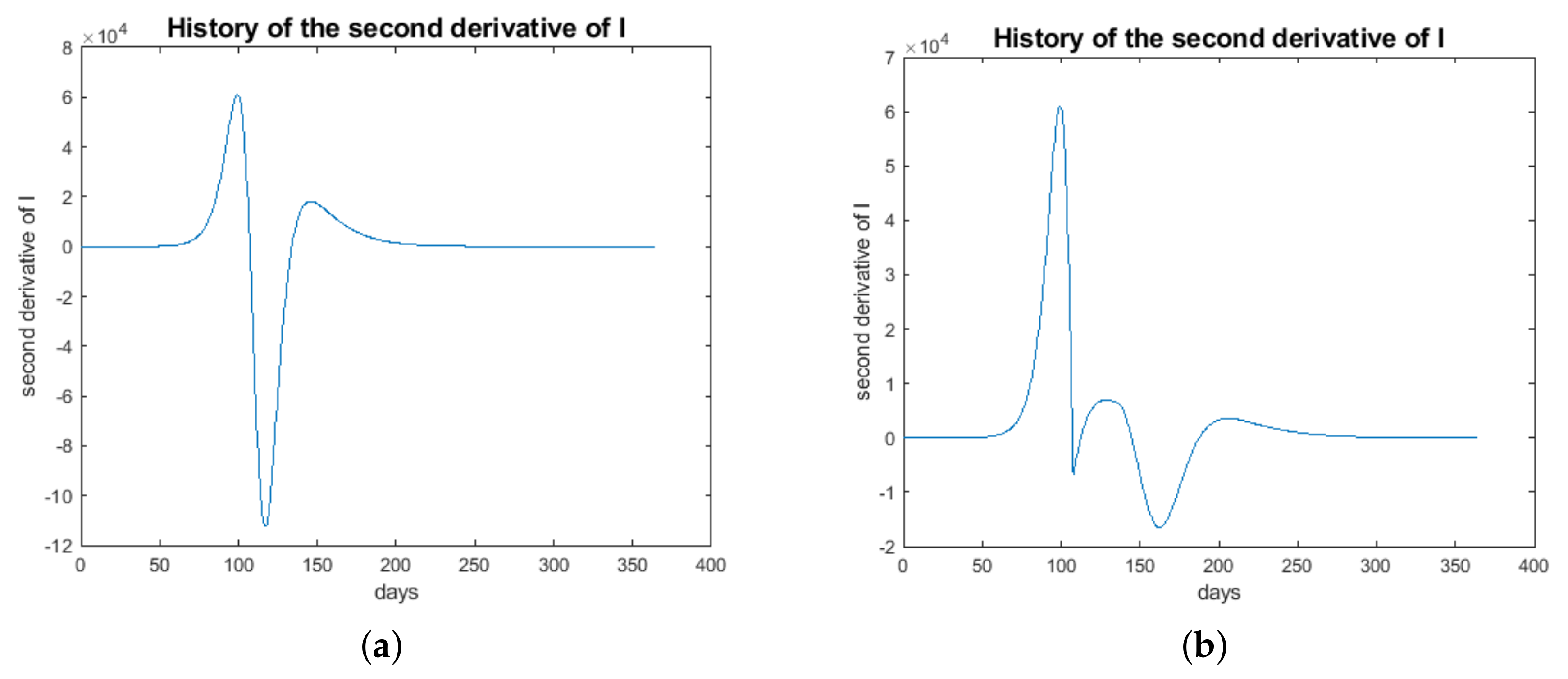
These are the points in time where the curve of I changes from a convex to a concave behavior or vice versa. The convexity or concavity can be controlled by the second derivative of $I\left(t\right)$.

Let us consider Equation (2). By differentiation of (2) and the use of (1), I get

$$\begin{array}{cc}\frac{d^{2}I}{d{t}^2}\hfill & =\frac{\beta }{N}\frac{dS}{dt}I+\frac{\beta }{N}S\frac{dI}{dt}-\gamma \frac{dI}{dt}\hfill \\ =& -{\frac{\beta }{N}}^{2}S{I}^2+(\frac{\beta S}{N}-\gamma )(\frac{\beta S}{N}-\gamma )I\hfill \\ =& [{(\frac{\beta S}{N}-\gamma )}^2-{(\frac{\beta }{N})}^{2}SI]I.\hfill \end{array}$$

With that, the I-curve will change from convex to concave if the relation

$${(\frac{\beta S}{N}-\gamma )}^2-{(\frac{\beta }{N})}^{2}SI<0⟺I>\frac{{(\frac{\beta S}{N}-\gamma )}^2{N}^2}{{\beta }^{2}S}$$

(7)

is valid. The switching time follows

$$t_0=\underset{t}{min}\{t>0,I\left(t\right)>{(\frac{\beta S\left(t\right)}{N}-\gamma )}^2{N}^2)/\left({\beta }^{2}S\left(t\right)\right)\}.$$

(8)

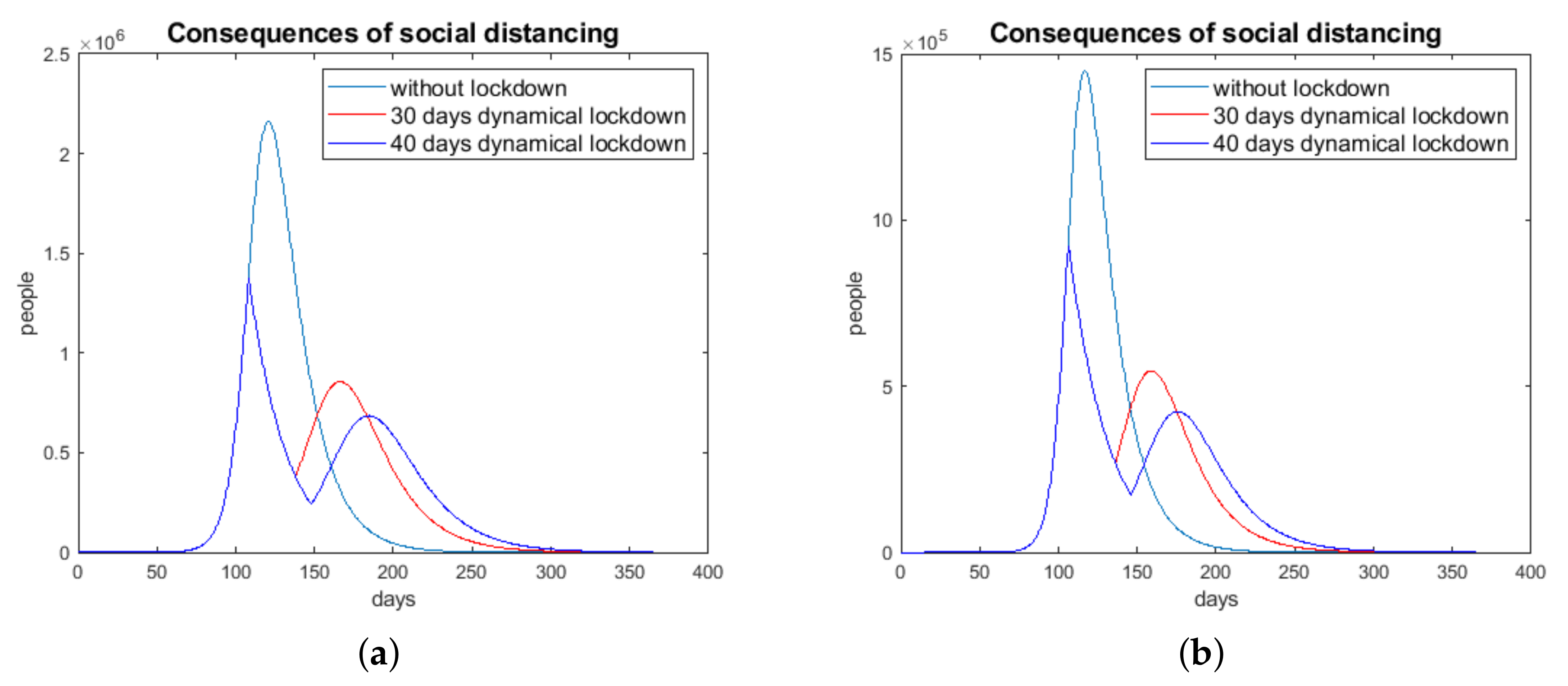
A lockdown starting at $t_0$ (assigning ${\beta }^{*}=\kappa \beta$, $\kappa \in [0,1[$) up to a point in time $t_1=t_0+{\Delta }_t$, with ${\Delta }_t$ as the duration of the lockdown in days, will be denoted as a dynamical lockdown (for $t>t_1$, ${\beta }^{*}$ is reset to the original value $\beta$).

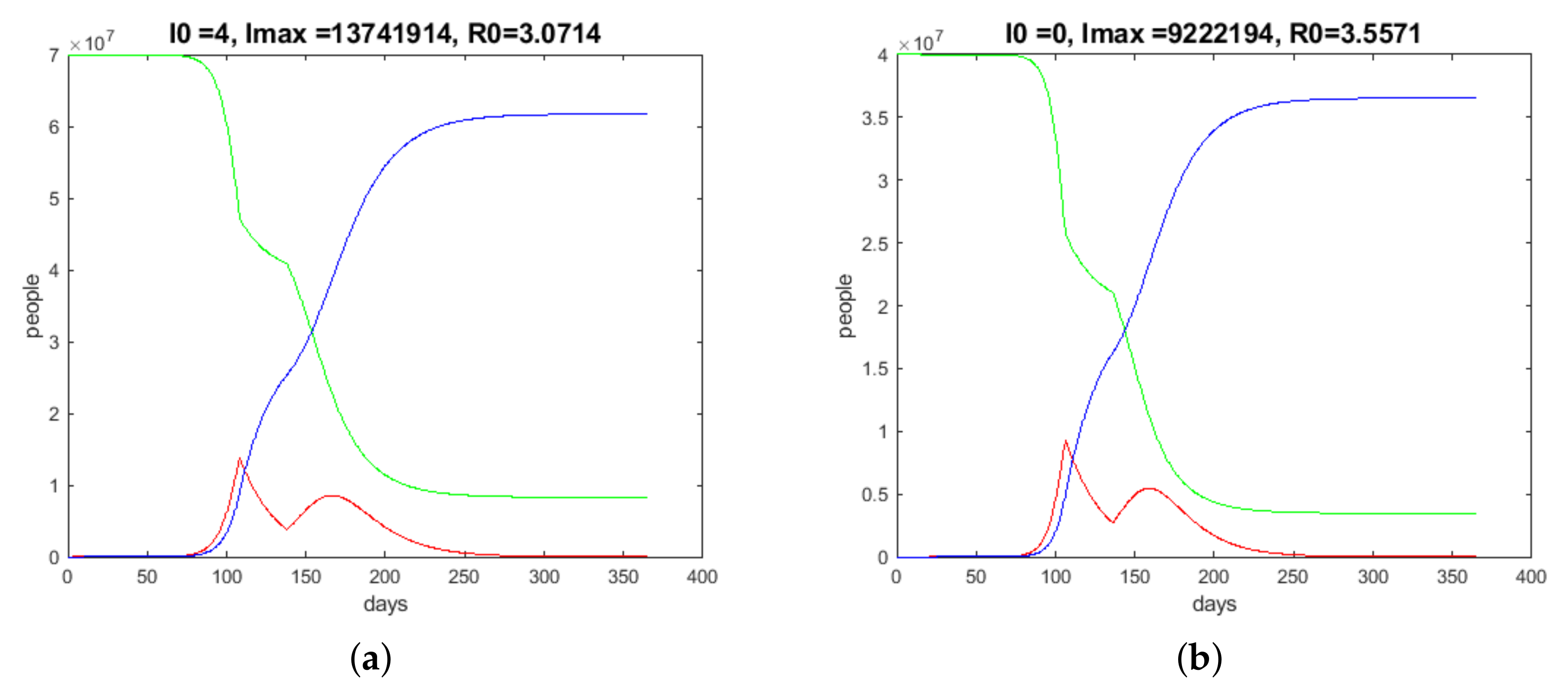
$t_0$ indicates the point in time up to which the growth rate increases and after which it decreases. Figure 8a shows the result of such a computation of a dynamical 30-days lockdown. I obtained $t_0=108$ ($\kappa =0.2$). The result is significant. In Figure 9a, a typical behavior of $\frac{d^{2}I}{d{t}^2}$ is plotted (in Figure 9b, $\frac{d^{2}I}{d{t}^2}$ in the dynamical lockdown case).

The result of a dynamical 30-day lockdown for Spain is shown in Figure 8b, where I found $t_0=106$ ($\kappa =0.2$).

Data from China and South Korea suggest that the group of infected people with an age of 70 or more is of a magnitude of 10%. This group has a significantly higher mortality rate than the rest of the infected people. Thus, I can presume that, as a high-risk group, $\alpha$ = 10% of I must be especially sheltered and possibly medicated very intensively.

Figure 10a shows the German time history of the above-defined high-risk group with a dynamical lockdown with $\kappa =0.2$ compared to the regime without social distancing. The maximum number of infected people decreases from approximately 1.7 million people to 0.8 million in the case of the lockdown (30-day lockdown).

This result proves the usefulness of a lockdown or strict social distancing during an epidemic disease. I observe a flattening of the infection curve as requested by politicians and health professionals. With strict social distancing for a limited time, one can save time to find vaccines and time to improve the possibilities of helping high-risk people in hospitals.

To see the influence of social distancing, I look at the Spanish situation without a lockdown and with a dynamical lockdown of 30 days in Figure 10b ($\kappa =0.2$) for the 10% that includes high-risk people.

The computations with the $SIR$ model show that the limited social distancing with a lockdown will be successful with a start after a time greater or equal to $t_0$, found by the evaluation of the second derivative of I (formula (8)). If the limited lockdown is started at a time less then $t_0$, the effect of such social distancing is not significant.

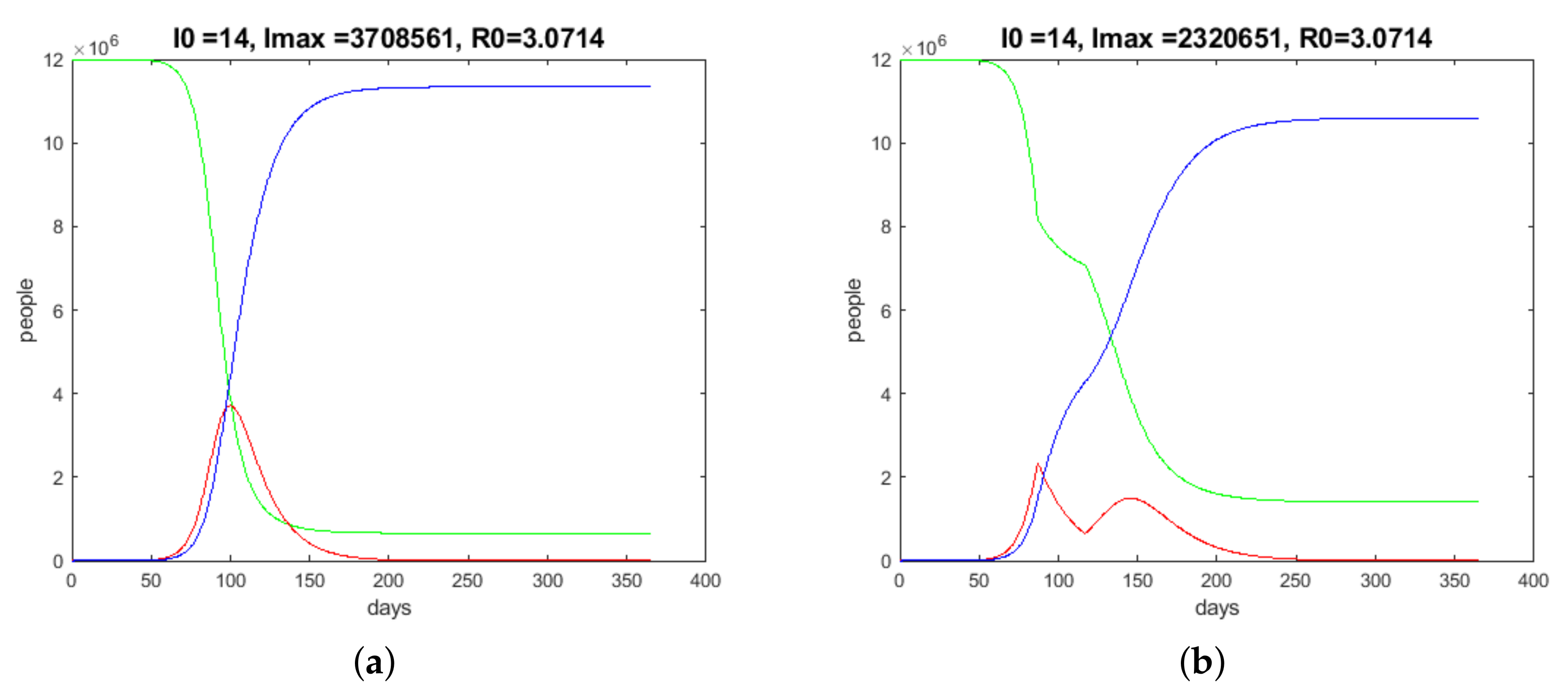
Bavaria is one of the origins of the German pandemic and is still under strict observation. Therefore, I will consider the simulation results for this German hotspot. I use $\beta =0.215$ and $N=12$ million as parameters. In Figure 11 the results for one year without and with lockdowns are shown.

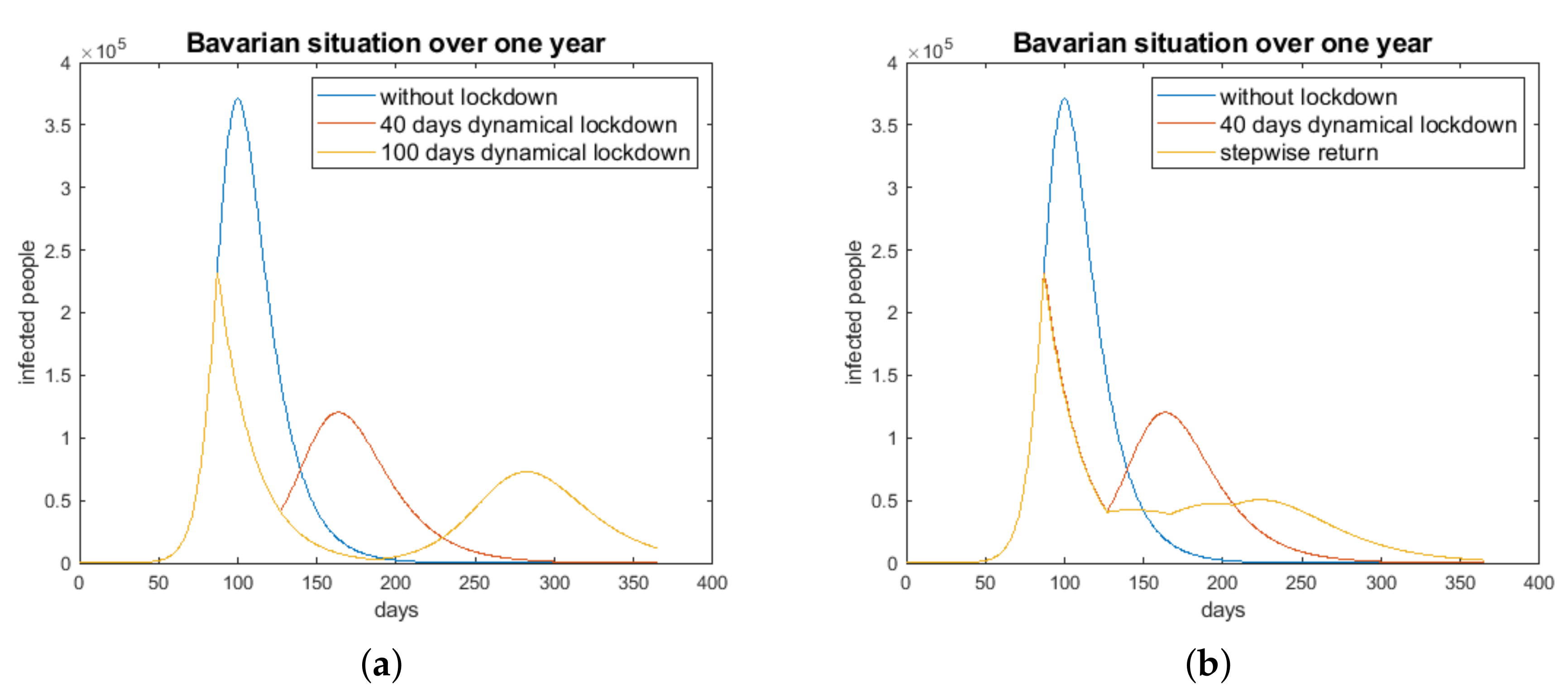
In Figure 12a, the consequences of a 40-day social distancing/dynamical lockdown for the development of the number of high-risk infected people are shown. Because of the increasing number of infected people after the 40-day lockdown, I simulated a step-wise return to normality. After the 40-day lockdown, two 40-day periods follow with 60% and 80% of normality, respectively. The result of this simulation is shown in Figure 12b.

The results for Bavaria with the considered step-wise lockdown can be passed to other regions or countries with pandemics. Such a strategy should be preferred instead of a complete return to normality after rigorous social distancing.

If I write (2) of the $SIR$ model in the form

$$\frac{dI}{dt}=(\kappa \beta \frac{S}{N}-\gamma )I,$$

I realize that the number of infected people decreases if

$$\kappa \beta \frac{S}{N}-\gamma <0⟺S<N\frac{\gamma }{\kappa \beta }$$

(9)

is complied with. The relation (9) shows that there are possibilities for the reduction of infected people to be inverted and the medical burden to be reduced.

(a)

The first possibility to decrease the number of infected people is the reduction of the infection rate $\kappa \beta$. This can be achieved through strict lockdowns, social distancing at appropriate times, or rigid sanitary measures.

(b)

The second way consists of the reduction of the stock of the species S. This can be achieved through immunization or vaccination.

(c)

The isolation of high-risk people (70 years and older) is another possibility for the reduction of the number of infected people. In addition, positive tests for antibodies reduce the stock of susceptible persons.

If there is quantitative information on the isolation of infected people through quarantine, the $SIR$ model can be extended by a species X, which quantifies symptomatic and quarantined infected people. This was considered in [2] for the Chinese province of Hubei.

6. Discussion and Conclusions

In this paper, I used a modified $SIR$ model to describe the progression of the COVID-19 pandemic. I find that the timing of the lockdown is crucial in the progression of a pandemic. It could be shown that a very early start of limited social distancing measures of a period of $\Delta t$ days leads only to a displacement of the climax of the pandemic, but not really to an efficient flattening of the curve of the number of infected people.

The intervention measures are more efficient, and one can observe a descent in the number of infected people if the social distancing is started beyond the dynamical lockdown time $t_0$. However, in this case, a second bump of the curve of infected people will also occur. A stepwise return to normality turned out to be the most efficient way to overcome the climax of a pandemic.

For the calibration of the $SIR$ model, i.e., the evaluation of the parameter $\beta$, the non-linear regression comes up with significantly better results than the log–linear regression. This is evident with the comparison of the graphs of the evaluated exponential functions.

It must be noted again that the parameters $\beta$ and $\kappa$ were guessed very roughly. In addition, the percentage representing the group of high-risk people, $\alpha$, is possibly overestimated. Depending on the capabilities and performance of the health systems of the respective countries, those parameters may look different. The interpretation of $\kappa$ as a random variable is thinkable, too.

I have to point to the second bump in the progression of the number of infected people as an important issue of limited lockdowns. This must be respected in all decisions of physicians and politicians in connection with the handling of the pandemic. The simulations for Bavaria pictured in Figure 12 show that there are return strategies that can reduce further ramps of the progression of the number of infected people.

In conclusion, it must be said that the results of the simulations using the $SIR$ model describe, in a way, the worst case. A lot of interventions made by politicians and physicians can disturb the progression of the pandemic in a positive way. However, not all measures and interventions can be described by $SIR$-type models. This allows the conjecture that the real pandemic will be weaker than the simulation results of the model.