Article

Simulating a Watershed-Scale Strategy to Mitigate Drought, Flooding, and Sediment Transport in Drylands

by
Connie M. Maxwell
1,2,*,
Saeed P. Langarudi
1 and
Alexander G. Fernald
1,2
1
College of Agricultural, Consumer and Environmental Sciences, New Mexico State University, Las Cruces, NM 88003-8003, USA
2
New Mexico Water Resources Research Institute, New Mexico State University, Las Cruces, NM 88003-8001, USA
*
Author to whom correspondence should be addressed.
Systems 2019, 7(4), 53; https://doi.org/10.3390/systems7040053
Submission received: 2 August 2019 / Revised: 1 November 2019 / Accepted: 5 November 2019 / Published: 28 November 2019
(This article belongs to the Special Issue System Dynamics: Insights and Policy Innovation)

Abstract

:
Drylands today are facing a landscape-scale water storage problem. Throughout the increasingly arid Southwest of the United States, vegetation loss in upland watersheds is leading to floods that scour soils and transport sediment that clogs downstream riparian areas and agricultural infrastructure. The resulting higher flow energies and diminished capacity to infiltrate flood flows are depleting soil water storage across the landscape, negatively impacting agriculture and ecosystems. Land and water managers face challenges to reverse the trends due to the complex interacting social and biogeophysical root causes. Presented here is an integrative system dynamics model that simulates innovative and transformative management scenarios. These scenarios include the natural and hydro-social processes and feedback dynamics critical for achieving long-term mitigation of droughts, flooding, and sediment transport. This model is a component of the Flood Flow Connectivity to the Landscape framework, which integrates spatial and hydrologic process models. Scenarios of support and collaboration for land management innovations are simulated to connect flood flow to the floodplains throughout the watershed to replenish soil storage and shallow groundwater aquifers across regional scales. The results reveal the management policy levers and trade-off balances critical for restoring management and water storage capacity to the system for long-term resilience.

Graphical Abstract

1. Introduction

Throughout the American Southwest and many global dryland regions, drought, increased flooding, and sediment transport are exacerbating landscape-scale water challenges [1]. Less winter precipitation and higher temperatures are diminishing snowpack storage [2,3], which results in less spring runoff quantities and flow durations for downstream water users [4]. Landscape losses of deep soils and vegetative cover in this region stem from historic overgrazing and fire suppression corresponding with climate effects that began in the late nineteenth century [5,6,7]. Rain and snow melt are no longer held by the soils and released slowly throughout the year; instead, they run off immediately in floods, resulting in catastrophic flows and severe erosion [5]. As vegetation on uplands decreases, hydrologic energy in valley bottoms increases, which increases scouring of floodplain vegetation and soil along the channel bottoms, entrenching flows in the valleys. Historically, floods along the many river networks were more connected to more richly vegetated floodplains [7]. When flood flow is connected to and can overbank onto floodplains, watersheds retain more their water and soil resources and result in multiple ecosystem services such as aquifer recharge, flood mitigation, vegetation productivity, and water quality treatment [8]. Agriculture traditionally and can again support this natural dynamic through watershed-scale systems of stormwater harvesting, with a general approach to spread flood flow onto floodplains employing practices such as flood irrigation. This management approach provides critical functions for long-term resilience in that it maintains the buffering capacity to drought, flooding, and erosion challenges [9] and results in infiltration into shallow groundwater aquifers [10].

1.1. Connectivity Processes Drive Dryland Landscape Dynamics

To achieve transformation of the landscapes and the communities that rely upon them to a resilient state requires collaborations of integrated management systems and disciplines across the scales [11]. To achieve such holistic land management requires developing common understandings of the system dynamics, the functional as well as the structural attributes of a system, which is often described as restoring the natural or biophysical functions and processes [12,13], or a process approach [14]. A resilient system can then be characterized and assessed by the processes and feedback loops that propel a system across a critical threshold to a system state that achieves desired functional goals [12,15]. Despite a general recognition of the importance of function throughout natural system disciplines, most approaches still assess natural systems from only a structural perspective, and many disciplines face challenges in taking a process approach due to the difficulties in conceptualizing and measuring certain processes [12,16]. An additional obstacle to a holistic system understanding is that the boundary of the system that reveals the dynamics is often divided; for example, upper watershed managers are not commonly in collaboration with downstream community efforts to address flooding and water scarcity issues. Current approaches to flood risk mitigation commonly do not often look to upper watershed management as part of the solution. “Mono-functional” flood control infrastructure (FCI) approaches often limit considerations of the surrounding natural system [17,18]. The goal is typically to control flooding through restricting area for river flow, such as using levees to protect floodplains under use. These spatial restrictions, however, decrease the buffering capacity of flooding processes and the overall system resiliency, which increases our vulnerability to catastrophic failures [17,19,20]. As increased flooding exposes these vulnerabilities, calls are emerging for process approaches on watershed scales, often termed eco-engineering approaches or nature based solutions [21,22], to adapt the socio-natural systems to flooding processes within the flood control disciplines [23]. A few programs under development have adopted these approaches, such as the “Room for the River” in the Netherlands [21,24,25,26].
Connectivity in watershed systems is emerging as a process that organizes dryland landscapes and is thus useful for revealing dryland dynamics [15,18,27,28,29,30,31,32,33]. Practitioners that developed connectivity as a tool for dryland watershed restoration placed the relationship between structure and function as a central perspective [15,18]. The dryland connectivity conceptual framework defines connectivity as the extent to which materials such as water, nutrients, and organisms can move, spread, or be redistributed from one place to another within the landscape [15,34]. Quantifying the connectivity and disconnectivity attributes can determine the condition of the watersheds and characterize the flux dynamics [30,31].
A critical driver of watershed conditions are the connectivity conditions of valley bottoms where water and other flows are concentrated throughout the watershed. When hydrologists refer to hydrologic connectivity, they are often referring to longitudinal connectivity, i.e., how fast flow proceeds to the watershed outlet [30]. An overall restoration strategy is to increase lateral connectivity, whereby channel flows are connected and able to flow laterally onto the adjacent floodplains [35]. This reconnection of the flow to the floodplain can address the extensive problem of increased hydrologic energy with scouring peaks of flow, as shown in Figure 1. More of the watershed would serve as a runoff sink, and less as a runoff source, with more water retained and overall storage increased [36]. An increase in lateral connectivity throughout a watershed increases the area of runoff sinks by spreading and slowing the flow, recharging soil storage capacity, and supporting vegetation productivity. Vegetation then provides the feedback function of increasing infiltration and water holding storage capacity through increasing surface roughness, introducing soil pathways, and increasing organic matter into the soil [37].
This dynamic is well-understood in perennial river ecosystems [38], but often overlooked in the upland (often managed grazing) systems, which contain the intermittent headwater valley bottoms (here, intermittent includes all temporary waterways, both intermittent and ephemeral). Intermittent systems, however, have unique ecosystem dynamics and require distinct management, monitoring, and research approaches [39,40]. These critical conduits of water, energy, material, and organisms support high biodiversity and important ecosystem processes [41]. A valley bottom system of well-connected channels to floodplains throughout the landscape, including the intermittent systems, serves as the buffer against both flooding and the effects of growing aridity [41].
For long-term resiliency, the natural system requires management of the connectivity of flood flow to the floodplains throughout the landscape to mitigate hydrologic energy. The slowing of hydrologic energy has the potential to result in replenishing soil storage and groundwater systems, which provides critical buffers against disturbances. This was the deciding factor for the boundary of this work. Other practices could contribute to the overall objectives, such as aquifer storage and recovery (injection wells) increasing groundwater storage [42]). However, targeting the existing management systems and incorporating floodplain reconnection restoration practices into daily activities of land managers across the landscape has the potential to have the furthest reach [43]. Floodplain reconnection is still not widespread, but it gained global recognition for its ability to control floods through restoring floodplain functions that yield multifunctional social and ecological benefits [25,44,45,46,47,48,49]. Many traditional and innovative land management practices can address these natural processes and functional goals of connecting flood flows to floodplains, with different practices appropriate for varying local conditions and dynamics, particularly for differing scales and hydrologic energy conditions. These include flood or spate irrigation [9,50,51], terraced agriculture [52], riparian buffers that filter and slow flow [53,54], and porous large wood and other debris and rock structures in both perennial and intermittent flow systems that slow but do not impound flow, mimicking beaver structure functionality [30,55,56,57,58,59,60,61,62]. All of these ultimately modify the connectivity on the landscape to increase vegetation and capture litter and nutrients, with the term “conmods” [15] coined to describe them.

1.2. A Systems and Action Research Approach

To understand the processes and dynamics in complex systems, systems science approaches fulfill a crucial function by characterizing the key drivers and relationship dynamics that determine system states over time. System dynamics (SD) modeling approaches offer unique abilities to characterize the effects of key feedback loops and quantify their magnitudes in simulation models, and to assess potential alternative future scenarios [63,64,65,66]. Many hydrologists recognized that social system feedbacks are essential for assessment of hydrologic systems [63,66,67,68], and hydrologists and other scientists in socio-environmental disciplines of socio-hydrology and hydro-sociology took up system dynamics approaches to understand the socio-natural system interactions, as “linear causal thinking cannot address complex challenges adequately” [69]. Hydrologists also took up SD modeling approaches to develop integrated water resources and watershed management approaches [69,70,71,72].
A systems approach enables revealing underlying dynamics that are fundamental to many systems, as well as generalizable innovative alternative management and scenarios that can transform them. Research in systems thinking identified that a core or generic set of “archetypes” can be found in many systems which are classifications of structures responsible for generic patterns of behavior over time [73,74]. Wolstenhome defines the most generic or basic archetypes as “underachievement”, “out of control”, “relative achievement”, and “relative control” [73]. A generic structure such as the model described in this work typically results in dynamics that correspond to several archetypes over the course of the model run. While it is outside of the scope of this article to map each dynamic’s corresponding generic archetype, this work did aim to explicitly address a widespread land management challenge that is one manifestation of the “tragedy of the commons” archetype. This is a commonly identified multiple-dynamic archetype where collective management tends a common pool resource system toward collapse. Each individual actor has an incentive to outcompete others by increasing his or her extraction of resources, leading to the reduction of resources below the levels of what is sustainable for the group as a whole [75]. In the system addressed by this work, interconnected resources across the landscape are being depleted. Management such as overgrazing in combination with increased occurrences of droughts resulted in over-extraction of the upland vegetation system. Addressing this root cause through spreading flood flow onto floodplains to support increased vegetation along upper watershed valley bottoms has cascading resulting effects of decreased flooding, increased infiltration, and an increase in an alternative water supply. This approach protects resources, infrastructure, and can help address surface water availability challenges that have increased groundwater reliance, a resource under the threat of collapse. Potential solutions require or can be more effective with a response archetype that fits into the category of “seeing and acting holistically” [73].
This management and policy approach is informed by collaborative action research and socio-ecological science (SES), approaches that have identified underlying principles that can thwart the tragedy of the commons. Current efforts to further understandings of “usable” science was long the terrain of the discipline of “action research”, where the scientific efforts are defined by communities’ actual problems and the need for collaborative efforts to address them [76,77,78]. A central tenet of action research that can be facilitated by SD modeling is that collaborative experimentation is critical to achieve any sustainable socio-environmental system transformation [43,77,79,80,81,82,83]. Enacting pilot studies and experiments can be conducted as scenario testing with a broad range of stakeholders and interdisciplinary scientists. These experiments both build the social capacity to innovate in the face of complex challenges and create models that enable society to visualize and integrate alternative management into daily life [77,83]. Scenario-testing also accelerates the refining of strategies that can be tested on the ground. A sociologist posited in the 1940s that, because these are complex systems, “if you want to know how things really work, just try to change them” [84]. As Ostrom showed, the tragedy of the commons and the incentives for individuals to compete in the depletion of common resources to catastrophic result is a dominant driver across societies, but not an inevitable one [83].

1.3. Main Aim of Work and Flood Flow Connectivity to the Landscape (FlowCon) Framework Summary

1.3.1. Main Aim of Work

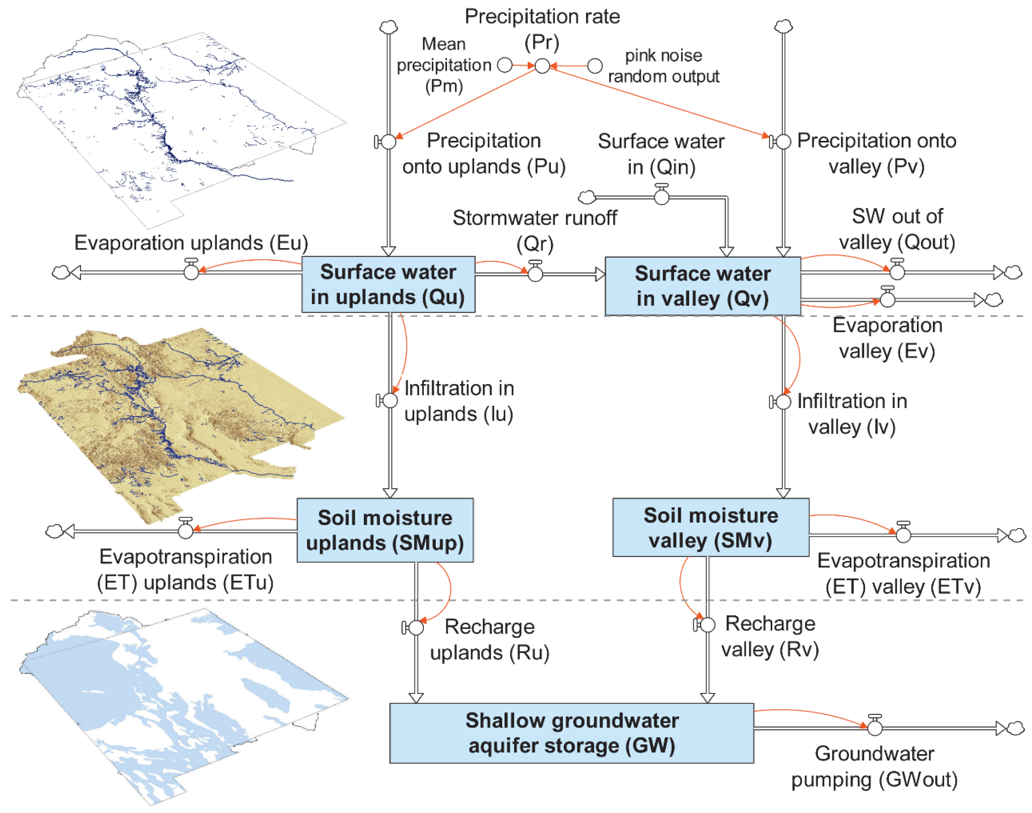
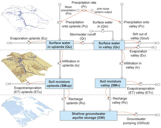
The occurrences of droughts and a general increase in aridity are drying upland soils, decreasing vegetation, and resulting in scouring floods across the American Southwest. The complexity and scale of ecosystems and management systems impede efforts to distill process-based solutions. The main aim of this work was to create a generalizable and adaptable integrative socio-environmental system dynamics model to facilitate development of regional collaborative approaches to define thresholds for resilient states. This model simulates an innovative watershed-scale stormwater harvesting and aquifer recharge strategy to reveal the extent of management (connectivity between flood flow and floodplains) required to reverse degradation trends. Key to this approach is simulating the water budget implications of alternate management strategies, which underlies the structure of the SD model (Figure 2). The scenarios were developed and iteratively modified to test the potential of achieving the following objectives: (i) the overall balance of system to manage flood flow/stormwater to increase downstream benefit while not negatively impacting downstream users, and (ii) to increase productivity/water availability to agriculture and reverse trends of groundwater storage declines.

1.3.2. Integration of Other Elements of FlowCon Framework

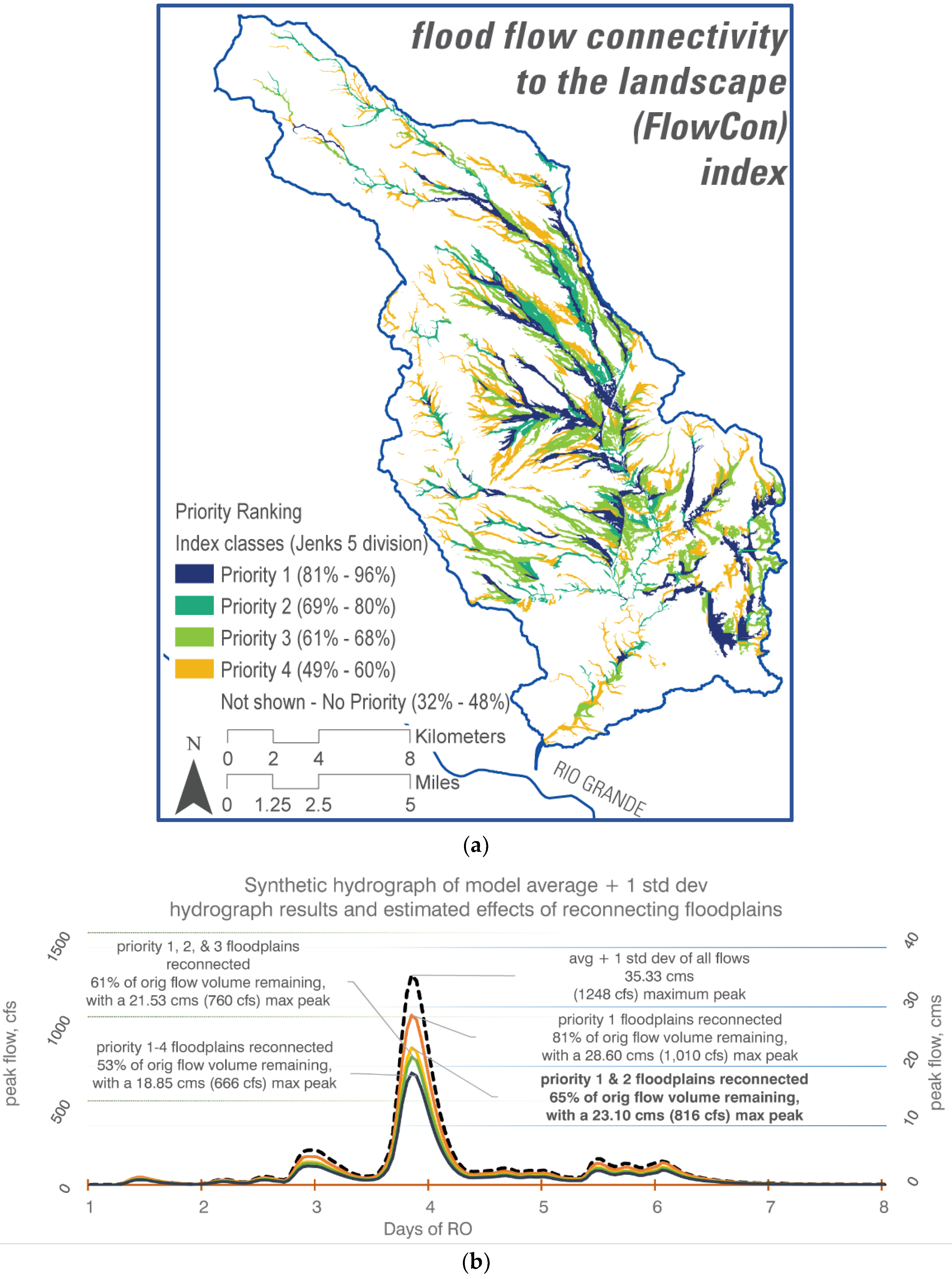
The SD model addressed in this article is integrated with the outputs of other Flood Flow Connectivity to the Landscape (FlowCon) framework models. These include a spatially explicit landscape indicator model and semi-distributed hydrologic models. Aggregated FlowCon outputs that are used as inputs to this SD model are shown in Figure 3a,b, and more details are provided in Section 2.1.3. The initial FlowCon framework models identify optimum locations and quantify the resulting benefits and extent of management and collaborative support required for restoration of the critical landscape processes. These target processes and functional goals that reduce hydrologic energy through increasing water retention, recharge, and vegetative productivity. Figure 3a shows the locations identified for reconnecting floodplains at varying levels of priority, and Figure 3b shows the effects on a synthetic hydrograph of executing the various levels. The top two priority levels shown were found to be the optimum levels for reversing degradation trends. The FlowCon framework provides a tool for use across disciplines to identify, quantify, and locate the critical process intervention targets for employing practices which then can be fit to local conditions.

2. Materials and Methods

Presented here is the system dynamics model of the FlowCon framework, a generalizable and adaptable model structure that includes the natural and management processes and feedback loops critical for achieving transformation of watersheds, mitigating droughts, flooding, and sediment transport over the long term. Note that stormwater is usually associated with urban areas, but here the strategy is to spread and slow flood flows across the landscape; thus, in upper watershed areas, we use the term flood flow, and, in the valley areas with more developed infrastructure, we use the term stormwater.

2.1. Model Structure

2.1.1. Generic Structure Generated from Southern New Mexico Site

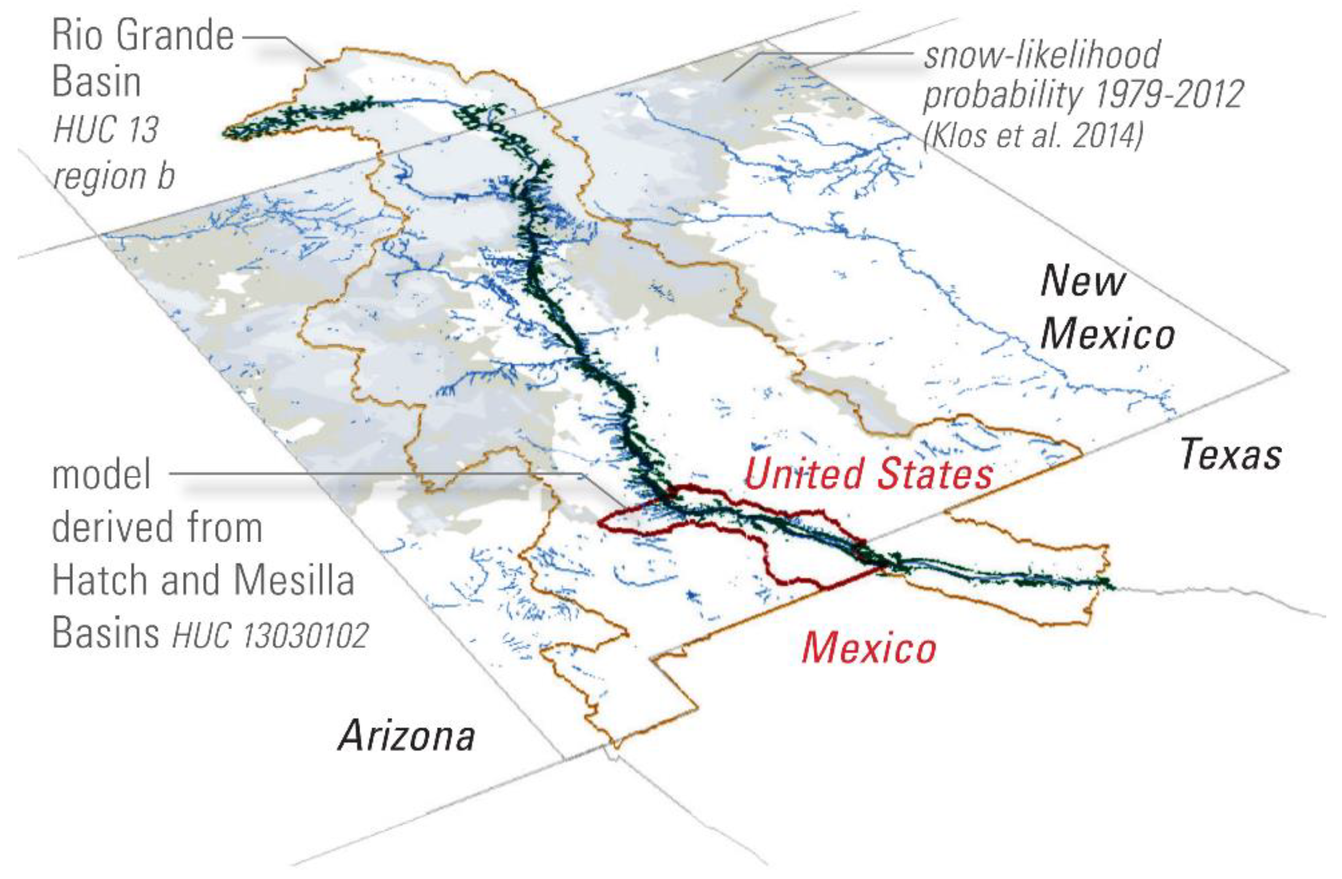
The FlowCon SD model was built in the Stella [85] software program; an image of the full model can be found in Appendix A (Figure A1), and a full list of equations can be found in Appendix B. The model data are derived from an area that faces significant drought, flooding, and sediment transport challenges. This basin in southern New Mexico, which lies directly upstream from Texas and Mexico, includes the Hatch and Mesilla Valleys (Figure 4). Using this real-world example tests the model’s outputs against our interpretation of history and the real system’s behavior. This generic structure can then be adapted to specific management decisions specific to a region under question and, thus, serves as a starting point for working with communities to experiment on potential management innovations.

2.1.2. Model Water Budget Approach

The essential structure of the model uses a water budget approach (Figure 3). Critical system conditions which can be assessed through a water budget have important effects on a community’s ability to mitigate drought, flooding, and sediment transport. The hydrology of the system is a major driver, both in terms of water quantity and distribution. A water budget as a management tool provides an estimate of the balance and distribution of water as it cycles through the system, and is most generally defined and calculated as the inputs minus the outputs are equal to the change in storage [86,87]. The budget estimates in this work allow for estimates of the effects on the water distribution and quantities from system innovations of interventions and the alternative land management simulated.
Hydrologists have utilized SD modeling approaches in conjunction with water budgeting to achieve greater system understandings. The New Mexico Water Resources Research Institute developed a Dynamic Statewide Water Budget system dynamics water budget model which produced outputs that this research relied upon for parameter ranges [88]. Modeling approaches that incorporate water budgeting allow for robust assessment of the competition between sectors and population clusters; for example, without policies that concretely identify agricultural needs, agriculture can be predicted to decline [89], an experience borne out over time [90,91,92]. Specific hydrologic processes modeled in system dynamics, including runoff, sediment transport, aquifer recharge, and aquifer storage and recovery, were shown to produce comparable results to other commonly used hydrologic models [42,93,94]). A critical link is to integrate with other modeling approaches, such as suites of models that include spatial modeling as this framework employs to facilitate the development of alternative watershed management strategies [94,95,96,97]. Integrating and linking spatially explicit and process-based models with integrative system dynamics frameworks was identified as critical to characterizing reference states and facilitate management planning [98]. Flooding risks motivated modeling approaches that explicitly address floodplain management as addressed in this work, although none to date included upland intermittent floodplain system interventions [95,99]. As Zischg [95] stated, floodplains are complex adaptive systems that are composed of co-evolving natural and human systems whose internal dynamics spawn emergent behavior that influences future risk pathways. These behaviors and management strategies include trade-offs between upstream and downstream users and the collective shouldering of risk. Baldassarre et al. [99] showed that, while human–water systems can be described as coupled, the two sides are not discretely distinct, and the attempt to describe the relationship between the systems is key to yielding innovative findings; in their example, the relationship between development aspirations in floodplains and the risks of flooding damage was described.

2.1.3. Model Boundary, Assumptions, and Inputs from Other FlowCon Framework Models

The boundary of the model is determined by the purpose that it serves, which in this work includes the extent of the system that reveals high-leverage management options for achieving long-term mitigation of droughts, flooding, and sediment transport. Table 1 summarizes the model boundary by distinguishing endogenous (calculated and affected by other variables within the model) and exogenous variables (inputs not changed by other model variables). Included as well is a list of variables that could have potentially been in the model but are excluded due to them being outside of the scope and focus of this research. The parameters used in this model were the scenarios of extent of floodplain connectivity that would result in mitigation of hydrologic energy to achieve the multifunctional ecosystem service benefits, increasing water availability, reducing sediment transport, and increasing productivity. This model enables projections of management of four main conditions: (i) the effect of water availability on agriculture that can increase or protect productivity, (ii) the balance of surface water between the upland and valleys below, (iii) the spreading of flood flow which enables the reduction of groundwater pumping (in-lieu recharge) [100], and (iv) the extent to which the interventions affect downstream users.
Outputs from other FlowCon framework models were used as input parameters to the model (the major parameters are noted in Table 1). Utilizing other FlowCon framework analyses allows this aggregated SD model to benefit from analysis that is often best conducted spatially across the scale of the study boundary. The linking of spatial and process-based models is an important expanding area of work due to the unique qualities and management needs of particular areas of the landscape, such as the differences in infiltration rates of uplands, upland floodplains, and wide farming valleys [98]). A significant feature of the FlowCon framework is the delineation of the upland floodplains (using Topographic Wetness Index (TWI) values correlated to valley bottom and channel contours [101,102]) and the subsequent spatial and hydrologic modeling that characterized and estimated the dynamics of the flow as it courses through the upland valley bottoms and the benefits of reconnecting that flow to the floodplains. The floodplain reconnection benefit analysis served as the intervention targets for the tested scenarios for this model.
The overall FlowCon framework includes this SD model, which integrates data from the suite of the three other models. The first is a spatially explicit GIS-based landscape and hydrologic indicator model using remote sensing inputs (fine-scale 4.5 m Digital Elevation Models (DEMs) [103] and observed radar precipitation inputs (NEXRAD) [104]), to produce a newly created expected wetness index (EWI). The EWI used here synthesizes the effect of precipitation intensity and antecedent wetness conditions, but has the potential and is currently being investigated to include vegetation density and pattern indicators using multi-spectral inputs [105]. The second model is a semi-distributed hydrological model using the SCS curve number (CN) method [106] in the HEC-HMS package, a commonly used tool by flood mitigation engineers [107]. The inputs of this model (CNs) are modified by the EWI inputs and calibrated by gauge data to quantify the locations, magnitudes, and frequencies of flow, and used to create a synthetic unit hydrograph from a series of actual rain events. The third model is a newly created hydraulic channel and floodplain network routing model in Excel. This model uses the hydrologic model results to distribute the runoff onto a finer scale, estimate the flow mitigation benefits from managing connectivity in optimum locations, and produce the spatially explicit FlowCon data. Several scenarios are tested to determine the extent of intervention required to address the functional goals. The results are then projected back onto the GIS-based landscape and hydrologic indicator model maps for use by the land managers.

2.1.4. Calibration, Validation, and Confidence Building Tests

The model successfully passed almost all conventional confidence building tests, including unit consistency, integration error, boundary adequacy, structural assessment, parameter assessment, behavioral anomaly, parameter sensitivity, and extreme conditions. On the topic of confidence building tests in system dynamics, refer to Sterman (Chapter 21) [108] for an exhaustive list, Barlas [109] for a methodological discussion, and Langarudi and Radzicki [110] for a practical example and guidelines. Unit consistency and integration error tests are straightforward procedures performed through Stella’s built-in features. The boundary adequacy test was conducted by examining the impact of each additional structure on the model’s behavior. The results indicated that all the endogenous variables were significant for the purpose of the study. Structural and parameter assessments were iterative processes which actually comprised the main model development phase. The majority of the logical structure of the model is explained in Section 1.1. The feedback structures and the parameters feeding them consist of local knowledge, literature, and technical estimations as described above throughout Section 2.1. At each stage of development, the model was tested for its behavior. It is normal that some anomalous behaviors appear at early steps, but they are fixed by modifying the structure. The same procedure was followed for parameter sensitivity and extreme condition tests which helped to identify a few flaws in the model structure. As an example, groundwater availability (GWa) and stormwater (SW) availability (Qa) were added to the model as first-order controls to prevent the water stocks from going below zero in extreme situations. These tests (especially parameter sensitivity) also helped to spot high-leverage points of the system, as discussed in detail in Section 4.
The model was also tested partially for policy sensitivity, which is further discussed in Section 3 and Section 4. The only tests that the model was not exposed to were family member and system improvement. Family member tests examine generalizability of the model by applying it to real-world problems that are similar to the original study case in terms of structure and characteristics. To pass the test, a recalibrated version of the model should be able to mimic those problems with reasonable accuracy. The system improvement test examines the robustness of the interventions proposed by the model in the real world. In this regard, the recommendations should actually be implemented in the real system, which is obviously yet to happen. Considering that the model is at its earliest stage of development, none of these tests could be realistically performed. They will, nonetheless, remain a priority for future research.
It is worth mentioning that the behavior reproduction test was not performed on the model in a conventional sense mainly due to the fact that historical data for the major variables were unavailable, such as evapotranspiration. The advantage to a water budget approach is that one can use several variables as closure terms, where the variables are calibrated to the known variable values. The advantage to the system dynamics model is that the inclusion of feedback gives added confidence, and these calibrations are often finely tuned and sensitive. Another reason for not pursuing a data-fitting exercise was that exogenous factors that might be significant but out of our endogenous scope were omitted. This reduces the model’s precision for point-by-point prediction but increases our ability to focus on key internal drivers. That is indeed why prominent system dynamics experts do not consider data-fitting as a strong validation test for SD models [111,112,113,114]. Therefore, the validity of our model relies heavily on the accuracy of its own internal feedback structure and data inputs that set its initial conditions. If the internal structure is deemed sound, then higher confidence can be placed in the outputs. In fact, the model’s outputs were reviewed by local domain experts and their general plausibility was approved.

2.2. Upland System to Support Ranchers to Increase Vegetation

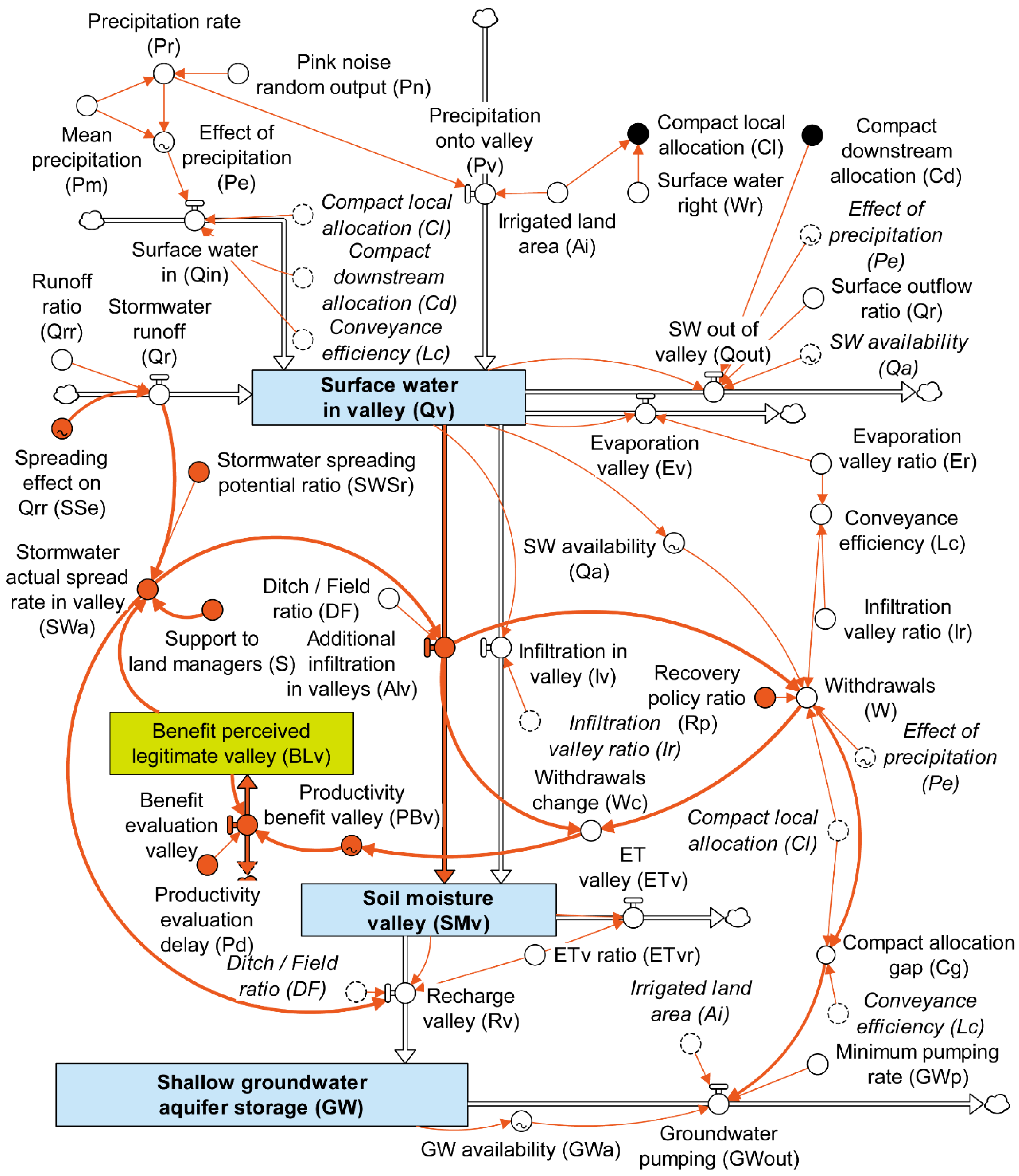
The SD model includes both the existing system and the scenarios of spreading flood flow and storm water, which are indicated in the model by variable shapes filled with dark-orange and bold connectors, as can be seen in Figure 5 and Figure 6. The upland system is shown in Figure 5, with the corresponding downstream valley section in Figure 6. The water “into” the system, precipitation (Pu), falls onto the landscape and produces surface water (Qu), which is then “lost” through evaporation (Eu), infiltration (Iu or AIup), or runoff (Qr). Normal infiltration (Iu) from Qu is estimated, as well as additional infiltration (AIup) from surface spreading (SSr). This infiltration fills the soil moisture stocks (SMup), which is then available for recharge (Ru) to the shallow groundwater aquifer (GW) and evapotranspiration (ETu). Increased ET availability increases vegetation coverage (VCa), which is checked by the additional vegetation increasing ET. VCa then provides productivity benefits to upland managers, which directly increases (or decreases) the ratio of surface spreading (the SSa portion of SSr), as does the support to land managers (S). Potential surface spreading of the landscape is specified in a ratio (SSr, here 0.2). This spreading then reduces the stormwater runoff to the valley system (Qr).

2.3. Valley System to Support Farmers to Increase Water Availability through Recharge and Stormwater Spreading

Figure 6 shows the valley system. The water inputs are Qr from the uplands, the precipitation (Pv) which falls onto the valley itself, and compact allocations (Cl and Cd, which are filled in black). Cl and Cd determine the surface water into the system that varies according to precipitation availability, which is modeled here as a distribution from an upland reservoir, a common condition. Water is lost through the surface water that flows out of the valley (Qout) which is affected by the downstream compact allocations, evaporation (Ev), evapotranspiration (ETv), infiltration (Iv and AIv), and groundwater pumping out (GWout) of the shallow groundwater aquifer storage (GW). Here, surface spreading of stormwater (SWSr) is either based upon a ratio (DF) of the ditch irrigation infrastructure to recharges directly into the GW, or is spread onto the fields. This increases the surface water withdrawal quantity (W) that the farmers get based upon their compact allocations (Cl) and availability (Qa and affected by Pe). Farmers pump a minimum quantity of groundwater (GWp) based on their water rights, and also pump an amount to match whatever surface water is not delivered (see further discussion in Section 4.1).

3. Results

Variability in the biosphere is effected by behavior in various time scales, including the period directly preceding it (or spatial period adjacent), which is a random behavior categorized as pink noise [115]. The precipitation inputs into the system were, thus, characterized by pink noise, and results in trends above and below the norm of various durations (see Figure 7). The pink-noise random variation used a constant seed in order to produce consistent quantities with all model runs allowing for scenario comparison. The mean was 10.41 inches (264 mm)/year with a standard deviation of 1.8 inches (45.72 mm).

3.1. Support

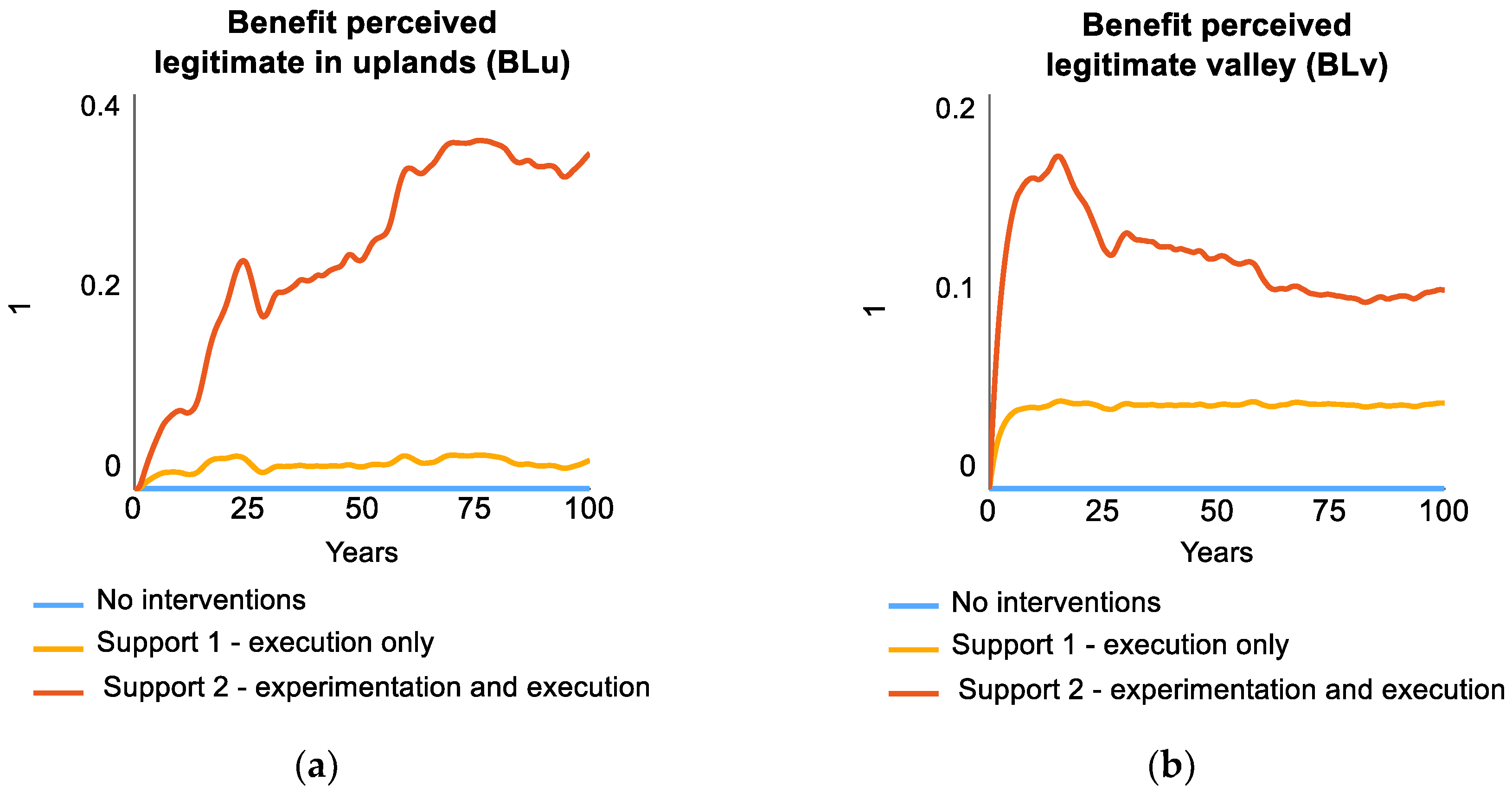
Support for managing flow connectivity to the landscape is provided by two functions, direct support to execute the new interventions and management, and support to managers to experiment with fitting the practices to their local conditions, thereby realizing more productivity benefits directly from the interventions. Three scenarios are shown in the results beginning in Figure 8: “No interventions” which represents the base case scenario with no additional flow connectivity management, “Support 1—execution only” which represents outside financial support to execute the new practices on a wider scale quickly, and “Support 2—experimentation and execution” which represents additional support for a phase of experimentation for a better fit to the local conditions to realize productivity benefits more quickly and to a greater extent, which leads to a perception of greater legitimacy of the practices. More upland interventions reduce the stormwater available for valley practices; thus, a tradeoff is that productivity benefits decrease in the valley with increased benefits in the uplands.

3.2. Strategy 1: Overall Balance of System Management of Stormwater to Increase Downstream Benefit While Not Negatively Impacting Downstream Users

Upland system. Mitigating high-energy flows that transport sediment downstream is a central strategy, which then yields additional critical ecosystem service benefits to the upland ranching managers. An optimal target identified by the FlowCon framework for this system (which would be different in other systems) is to reduce the runoff quantity by 35%, as that target correlates to sufficient reductions in the peak flows to achieve the desired functions. Approximately 15% of the diverted flow on average is infiltrated, therefore, to result in this reduction of runoff the initial targeted surface spreading water quantity is approximately 120,000 AF (Acre Feet). As shown in Figure 9a,b, surface spreading in the uplands (SSa) reduces stormwater runoff (Qr) to the targeted amount by the Support 2 scenario.
Valley farming system. Increasing water availability for the downstream farmers is the central valley goal. The valley system of farmers is downstream to the upland system and upstream to Qout. While stormwater runoff (Qr) is reduced by upland interventions, the combined effects are still enough to reverse the trend of shallow groundwater aquifer decline, as shown in Figure 10. While the differences might appear insignificant, typically only a ratio of the groundwater aquifer storage is usable and, as levels decline, the corresponding water quality generally also declines, decreasing that ratio. Note that each system would have different base conditions and different targets.
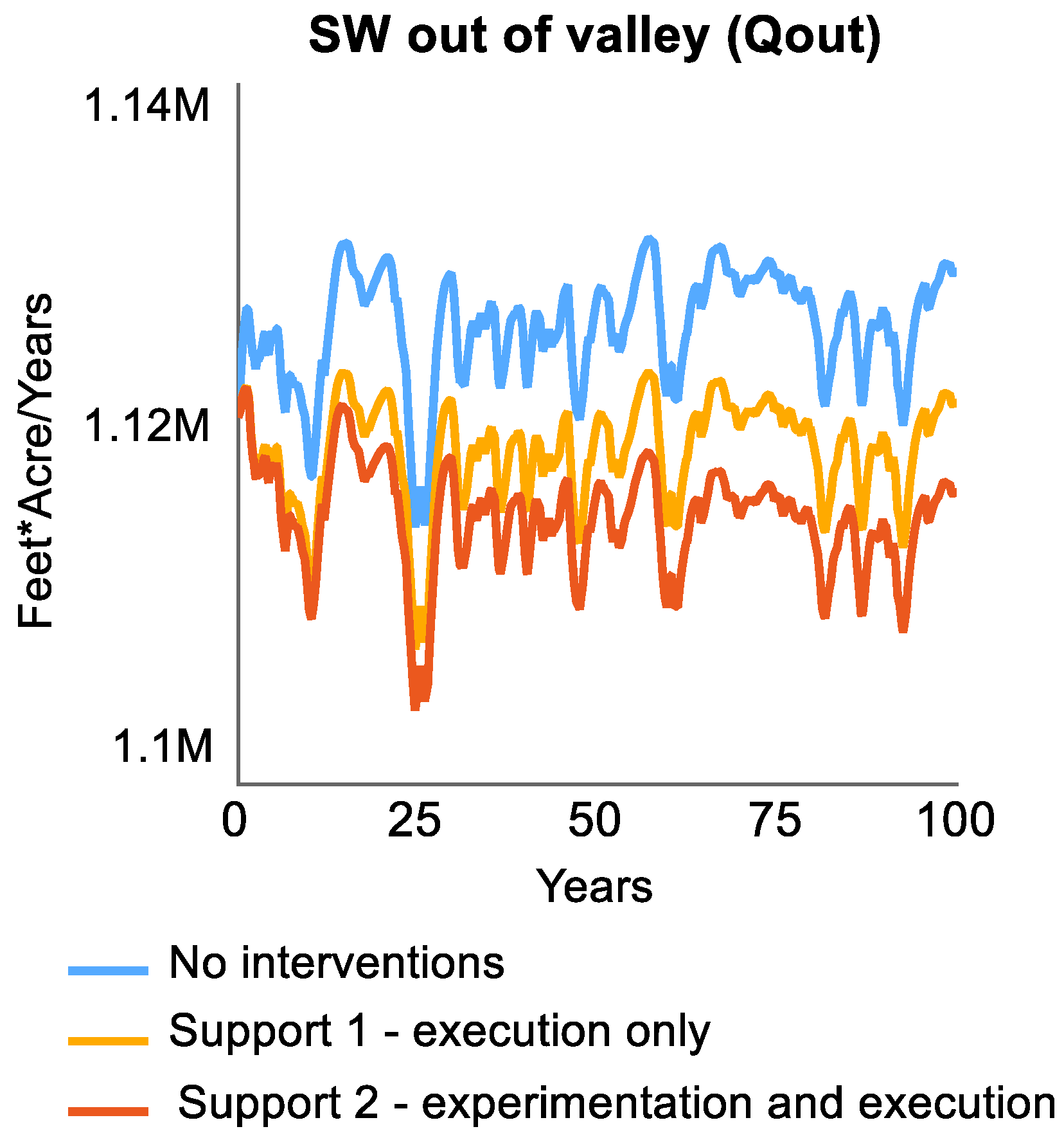
Downstream users. At the most downstream point in the model, the quantity of SW out of the valley (Qout) delivers the compact downstream allocation (Cd) to users downstream of the system (Figure 11). In dryland areas, this allocation is typically supplied by surface water that is distributed into the system from an upstream reservoir and, thus, the majority of the water supply is not from stormwater. Figure 11 shows that the Qout quantity does not change substantially, and it is well above the Cd amount of 679,000 AFY.

3.3. Strategy 2: Increase Productivity/Water Availability to Agriculture and Reverse Trends of Groundwater Storage Declines

Upland ranching system. The additional infiltration in the floodplains of the valley bottoms results in additional vegetation, as shown in Figure 12, which in turn fuels surface spreading (SSa) which produces additional infiltration (AIup) to the normal infiltration (Iu) in the valley (as shown in Figure 5).
Valley farming. The valley farmers’ production is directly related to water availability. As shown in Figure 13, withdrawals (W) increase with the stormwater spreading (SWa) interventions, reducing any surface water supply compact allocation gap, and thus reducing the need for groundwater pumping (GWout), known as “in-lieu recharge”. The recovery policy ratio (Rp) for farmers able to capture and reuse groundwater is 0.75. This resulting effect of increasing groundwater levels and storage benefits the valley farmers with greater water availability in the form of W. Both support scenarios shown in red and orange produce similar results.

4. Discussion

4.1. Scenarios for Achieving Transformation of Trends of Resource Declines

Two main critical policy/intervention dynamics in the uplands and valley management systems are addressed through highly aggregated support structures to land managers. As can be seen in the uplands structure in Figure 5, the benefits that the local managers would yield (BLu) is the more developed structure in the model. Those benefits ultimately support mainstreaming, the adoption of resilient practices into daily management [43], in these primarily range management systems. An increase in actual vegetation coverage represents forage increases, which is both the most critical productivity objective and the most challenging to achieve. Here, the innovation is to manage the range landscape through the critical driver of flood flow dynamics. Reconnecting floodplains would allow for two management improvements. Firstly, the larger floodplains can be developed as pastures are in irrigated areas providing direct productivity gains of grass responses, which can begin to be realized in the first season. Secondly, improved productivity in the floodplains would allow for more opportunity for longer recovery periods of upland rest from grazing. As raised earlier, floodplain reconnection is not a widespread resource management strategy, particularly in uplands, as the hydrologic energy behind flood flows is extensive, and ways to harness the water quantity without incurring damage from the energy represent a challenge. Support for land managers to experiment with fitting the practices to their local conditions is critical, and the details of the scenarios are discussed in further detail in Section 3.1. The complexity of every ecosystem and the management approaches and opportunities provide unique conditions and needs. Here, the support to experiment is represented by the reference mode of behavior of productivity benefit uplands (PBu) and the productivity benefit valley (PBv), as shown in Figure 14. The support scenario 2 experimentation to fit the practice to the local conditions would yield productivity benefits more quickly and to a greater extent, leading to a perception of greater legitimacy of the practices. Additionally, it would provide local collaboration, which would lead to increased innovation and greater adoption. The support scenario 1 of outside support to simply shoulder the management burden would experience a longer learning curve and greater adaptive management inputs to correct unintended consequences, yielding slower and less robust benefit yields over time. An important strategy is for the land managers to experience benefits as quickly as possible.
In the valley farming systems, the benefit modeled is the result of scenarios of an increase in water availability through stormwater spreading (SWa), resulting in both the shallow groundwater aquifer recharge and additional water supply directly to fields. The spreading results in additional infiltration (AIv), which then reduces the need for surface water withdrawals, which then reduces any potential water delivery gap (Cg), resulting in “in-lieu recharge”, i.e., less groundwater pumping (GWout).
Support to land managers (S) from outside the system represents the result of collaboration across scales and can represent a range of initial injections to sustained support. Initial injections are commonly in the form of financial and technical support through vehicles such as grants. Sustained support generally requires an ecosystem service payments approach where beneficiaries support, either directly or through the state, the land managers in shouldering the management burden over the long term. The structure in this model is a constant ratio of direct support to accomplish a ratio (20%) of the potential maximum amount of floodplain area that can be reconnected and the surface spreading potential ratio (SSr), which is 20% of the landscape; thus, the floodplains reconnected in this model represent 4% of the upland landscape.
Working landscape communities of rural farmers and ranchers likely require sustained support for planning, testing, installation, monitoring, and adaptive management phases. The initial responses of the system to the interventions in this model take into account that the interventions start on smaller scales and expand. It takes time, experimentation, and expertise to build innovative approaches. The support included here assumes a strategy of ecosystem service payments from downstream beneficiaries to addresses this issue [116]. This modeling framework can be used to identify the beneficiaries of an alternate scenario and develop a collaboration or negotiations to fund or incentivize the needed management changes. The typical application is that (in this case, downstream) beneficiaries of (upstream) restoration would pay a significantly lesser amount to address the problem before it develops. A prominent example is when farmers in upstate New York felt significant economic pressure to survive and responded with intensifying their farming and livestock management. By the end of the 1980s, the increased fertilizer use and general production intensification started contaminating the New York City (NYC) water supply. NYC’s Commissioner of Environmental Protection and Director of the Water and Sewer System, Albert Appleton, created an urban–rural collaboration to support farmers to voluntarily maintain sustainable practices in combination with purchasing and protecting key upstream properties [117]. As Appleton and others identified, the key for communities of any resource level, and particularly those with less than NYC, is to identify the costs of the problem and compare the costs of solutions to show evidence that they can legitimately address the problem over the long term.
In communities without significant economic resources, non-cash rewards show promise to have greater effect [118,119,120]. In New Mexico, as in many states across the West, water policy is driven by managers’ need to meet compact requirements, and allowing upstream managers such as ranchers to divert and infiltrate water unilaterally could threaten the ability to meet those requirements. Evidence of the application of these approaches where no downstream impairment occurs could open up opportunities for support for water management that increases landscape-scale soil and groundwater storage over the long term. Upon such evidence, water rights or water use through a water-banking program could be used as a non-cash reward.
Land restoration on a large scale could also be potentially fueled by carbon credit or tax systems. These systems would pay land managers to increase their vegetation productivity to result in increased carbon storage. Carbon is a measure of ecological conditions increasingly used by scientists and regulators globally. In California, the carbon credit market is currently funding restoration projects and, historically, the Chicago carbon market did as well. Studies showed how carbon markets could become significant incentives to fuel restoration [121]. A 2015 study determined that, while carbon markets alone would not likely incentivize farmers to convert to their fields to riparian floodplains, it could repay 100% of the costs to do so, showing the potential for a hybrid solution of riparian buffers and a significant fund source [122].
A basin-scale stormwater harvesting and recharge strategy is likely far less expensive than the “gray” or “hard” engineering approaches typically used for flood management infrastructure [123,124]), as well as yielding far more economically advantageous ecosystem services [123,125]. However, the management burden on the agricultural community would likely be significant, particularly in early experimentation and adoption. To realize innovations in management structures to the extent that can transform the natural systems to a resilient condition, support is critical. The action research approach of building collaboration within and across scales garners outside support for both shouldering the management burden and increasing innovation capacity to yield local productivity increases considered legitimate [11,77,126].

4.2. The Hydrology–Vegetation Feedback Dynamics

A system dynamics modeling approach and its ability to capture feedback dynamics is particularly useful for characterizing the strong link between hydrology and vegetation. In this model, the interventions result in changes in the landscape vegetation conditions over time, which then changes the landscape response to flood flows. Researchers linked threshold densities of dryland vegetation occurring in bands and patches to land productivity, carrying capacity, and resource health [15,127,128,129,130,131,132]. Reference conditions have greater vegetation density and diversity on connected floodplains than the adjacent hillsides [133,134]. The extent of floodplain vegetation density is, therefore, a key indicator of connectivity that has the potential to define thresholds for resilience in dryland systems. The hydrology–vegetation interactions are captured here with two main feedback dynamics. Firstly, additional water infiltrated resulting from the additional spreading of flood flows across floodplains (AIup) supports increased vegetation growth (VCa), which in turn supports additional infiltration (Ifp), i.e., a positive feedback loop (as can be seen in Figure 5 or Figure A1). Secondly, the increased vegetation growth is balanced by the function that the additional soil moisture available for evapotranspiration (ETup and Eta) is inevitably consumed by additional vegetation, providing a limit to growth. The spreading of flood flows occurs in the floodplains of the upland landscape, which has higher infiltration rates (Ifp) than the average of the landscape (If), allowing for separate functions to recognize discrete spatial dynamics.

4.3. Managed Aquifer Recharge to Reverse Groundwater Storage Declines

The storage and distribution of the water through river systems around the world are managed for downstream users. Agriculture has the greatest quantity needs and the greatest controls over what gets recharged back into the groundwater aquifer systems. The approach in this work assumes that providing agriculture with the ability to conduct the innovative practices of managed aquifer recharge (MAR) is the best approach to reverse the trends of declining groundwater storage in aquifers globally over the long term.
MAR refers most generally to the concept of land management with the purpose of recharging aquifers and includes a variety of practices, with the most common application being surface spreading [135]. Aquifer storage and recovery (ASR) is the term most commonly associated with MAR, yet this refers to a specific application which involves injection wells and rights for users to then recover the water through pumping and use. The approach here primarily looks at agricultural systems as the actors of MAR, although this model could easily adapt to incorporate other MAR techniques, such as ASR.
Generally, agriculture does not take advantage of stormwater flows, often due to water rights limitations, which are typically limited to the quantities of water distributed from reservoirs through water compact agreements. This model includes a dual system of stormwater and traditional use, whereby compact allocations drive the distribution of surface water upstream from the system, as shown in Figure 15. These allocations are affected by upstream precipitation/snowpack variability, where any quantity below a mean level set by the compact agreement reduces the allocation, as shown in Figure 15b.
Stormwater spread in this management and policy approach serves to balance the tendency to decline the groundwater levels. In the current system, supply to farmers are the withdrawals from surface water, which are initially the compact local allocation (CI) as reduced by the effect of precipitation (Pe) (as can be seen in Figure 6). The reductions from precipitation variability create a gap in the water right and what is allocated (Cg). This gap is generally filled by additional groundwater pumping (GWout). The stormwater actual spread (SWa) is the policy intervention, and it provides two functions for reversing shallow groundwater aquifer (GW) levels: recharge directly into the aquifer, and additional supplies of stormwater used for fields in lieu of pumping. Future work on the model intends to further develop the characterization of the contribution of recharge in the upland floodplains as subsurface flow to the valley shallow groundwater aquifer.

5. Conclusions

Many drylands globally are experiencing the tragedy of the commons dynamics found in the American Southwest, where management in the face of the disturbances (drought, flooding, and sediment transport) results in diminishing of natural resources and system “underachievement.” While this common system behavior is indisputably a powerful phenomenon, Ostrom proved that the dynamic can be thwarted through the collaborative actions of land managers across scales. This model proposes a land management archetype that fits into the category of “seeing and acting holistically” to restore socio-environmental capacity for resilience to the system. Flood flow is a powerful and underutilized leverage point in water-limited dryland systems. Transforming the management system to harness this opportunity on a large scale faces several challenges: what practices can successfully spread flood flow without incurring damage from the energy, who will do the work of installing stormwater harvesting practices across the scale of the landscape, and what will the incentives be? Ultimately, how could large-scale restoration realistically be achieved? This model provides a water management framework to estimate mitigating the trade-offs of upland ranching management using just enough upland flood flow to mitigate flood energy, while allowing enough to flow to the valleys to use for aquifer and in-lieu recharge. The ultimate model objective is the goal-seeking behavior of building both the natural system resource capacity and the social management system capacity to innovate, thereby achieving a resilient state. Managing flood flow connections to the landscape by slowing and reconnecting flow to floodplains mitigates hydrologic energy and results in replenishing soil storage and recharging groundwater systems, which provide critical buffers against disturbances, essential for long-term resiliency. The model is generalizable and adaptable to dryland working landscapes globally, and it serves as a collaborative starting point for working with land managers to both characterize the system under study and project scenarios of what leverage points will achieve the desired capacity-building goals. Nearly 40% of the global land surface is managed in agriculture, and, with innovative management of system functions, agriculture can revive traditional functions and once again become a system for recharging our aquifers and restoring our watersheds.

Supplementary Materials

The following are available online at https://www.mdpi.com/2079-8954/7/4/53/s1: A pdf image of the full model included in Appendix B and the model in the Stella software format.

Author Contributions

Primary conceptualization of policy, C.M.M.; development of natural system and management conceptualization, C.M.M., S.P.L., and A.G.F.; methodology, C.M.M., S.P.L., and A.G.F.; software, C.M.M. and S.P.L.; validation, C.M.M. and S.P.L.; formal analysis, C.M.M. and S.P.L.; investigation, C.M.M.; resources, C.M.M., S.P.L., and A.G.F.; data curation, C.M.M.; writing—original draft preparation, C.M.M.; writing—review and editing, C.M.M., S.P.L., and A.G.F.; visualization, C.M.M.; supervision, S.P.L. and A.G.F.; project administration, C.M.M.; funding acquisition, A.G.F.

Funding

This research was funded by the New Mexico Water Resources Research Institute general funds, the State of New Mexico Legislature NMWRRI2018 and NMWRRI2019, and the National Science Foundation Office of Experimental Program to Stimulate Competitive Research (EPSCoR) grant Award No. IIA-1301346.

Acknowledgments

The authors acknowledge the South Central New Mexico Stormwater Management Coalition and Elephant Butte Irrigation District for flow data and collaboration, as well as Babak Bahaddin, Holly Brause, Ashley Page, and Yining Bai for review of concept and model methodology, Jesus Figueroa and Adrienne Dawes for processing of data for the spatial and hydrologic models of the FlowCon framework, and the anonymous reviewers for their insightful and helpful comments for significant improvements to the manuscript.

Conflicts of Interest

The authors declare no conflict of interest.

Appendix A

The full model structure is shown here and is available online at the address included in the Supplementary Materials section above. The model equations are included in Appendix B.
Figure A1. Full model structure.
Systems 07 00053 g0a1

Appendix B

As addressed in the article, the model was built in the Stella software system [85]. The complete model equations per the Stella format are shown below.
The model has 76 (76) variables (array expansion in parens).
In root model and 0 additional modules with 0 sectors.
Stocks: 9 (9) Flows: 20 (20) Converters: 47 (47)
Constants: 23 (23) Equations: 44 (44) Graphicals: 10 (10)
Top-Level Model:
“Actual_vegetation_coverage_%_(VCa)”(t) = “Actual_vegetation_coverage_%_(VCa)”(t - dt) + (“ET_availability_effect_on_vegetation_(ETa)”) * dt
INIT “Actual_vegetation_coverage_%_(VCa)” = 0.25
UNITS: NDVInormal
INFLOWS:
“ET_availability_effect_on_vegetation_(ETa)” = (“Vegetation_coverage_expected_(VCe)”- “Actual_vegetation_coverage_%_(VCa)”)/”Vegetation_response_delay_(Vd)”
UNITS: NDVInormal/Years
“Benefit_perceived_legitimate_in_uplands_(BLu)”(t) = “Benefit_perceived_legitimate_in_uplands_(BLu)”(t - dt) + (“Benefit_evaluation_uplands_(Bu)”) * dt
INIT “Benefit_perceived_legitimate_in_uplands_(BLu)” = 0
UNITS: 1
INFLOWS:
“Benefit_evaluation_uplands_(Bu)” = ((“Productivity_benefit_uplands_(PBu)”- “Benefit_perceived_legitimate_in_uplands_(BLu)”)/”Productivity_evaluation_delay_(Pd)”)* switch
UNITS: Per Year
“Benefit_perceived_legitimate_valley_(BLv)”(t) = “Benefit_perceived_legitimate_valley_(BLv)”(t - dt) + (Benefit_evaluation_valley) * dt
INIT “Benefit_perceived_legitimate_valley_(BLv)” = 0
UNITS: 1
INFLOWS:
Benefit_evaluation_valley = (Productivity_benefit_valley- “Benefit_perceived_legitimate_valley_(BLv)”)/”Productivity_evaluation_delay_(Pd)”
UNITS: Per Year
pink(t) = pink(t - dt) + (update) * dt
INIT pink = scaled
UNITS: 1
INFLOWS:
update = gap/corr_time
UNITS: Per Year
“Shallow_groundwater_aquifer_storage_(GW)”(t) = “Shallow_groundwater_aquifer_storage_(GW)”(t - dt) + (“Recharge_valley_(Rv)” + “Recharge_uplands_(Ru)” - “Groundwater_pumping_(GWout)”) * dt
INIT “Shallow_groundwater_aquifer_storage_(GW)” = 20000000
UNITS: Feet*Acre
INFLOWS:
“Recharge_valley_(Rv)” = (“Soil_moisture_valley_(SMv)”+ “Stormwater_actual_spread_rate_in_valley_(SWa)”* “Ditch_/_Field_ratio_(DF)”)* (1-”ETv_ratio_(ETvr)”) [UNIFLOW]
UNITS: Feet*Acre/Years
“Recharge_uplands_(Ru)” = “Soil_moisture_uplands_(SMup)”* (1-”ET_upland_fraction_(ETup)”) [UNIFLOW]
UNITS: Feet*Acre/Years
OUTFLOWS:
“Groundwater_pumping_(GWout)” = “GW_availability_(GWa)”* ((“Minimum_pumping_rate_(GWp)”* “Irrigated_land_area_(Ai)”)+ “Compact_allocation_gap_(Cg)”) [UNIFLOW]
UNITS: Feet*Acre/Years
“Soil_moisture_uplands_(SMup)”(t) = “Soil_moisture_uplands_(SMup)”(t - dt) + (“Infiltration_in_uplands_(Iu)” + “Additional_infiltration_in_uplands_(AIup)” - “Recharge_uplands_(Ru)” - “Evapotranspiration_(ET)_uplands_(ETu)”) * dt
INIT “Soil_moisture_uplands_(SMup)” = 50000
UNITS: Feet*Acre
INFLOWS:
“Infiltration_in_uplands_(Iu)” = “Surface_water_in_uplands_(Qu)”* “Infiltration_upland_fraction_(If)” [UNIFLOW]
UNITS: Feet*Acre/Years
“Additional_infiltration_in_uplands_(AIup)” = “Surface_spreading_in_uplands_actual_(SSa)”* “Infiltration_floodplains_fraction_(Ifp)” [UNIFLOW]
UNITS: Feet*Acre/Years
OUTFLOWS:
“Recharge_uplands_(Ru)” = “Soil_moisture_uplands_(SMup)”* (1-”ET_upland_fraction_(ETup)”) [UNIFLOW]
UNITS: Feet*Acre/Years
“Evapotranspiration_(ET)_uplands_(ETu)” = “Soil_moisture_uplands_(SMup)”* “ET_upland_fraction_(ETup)” [UNIFLOW]
UNITS: Feet*Acre/Years
“Soil_moisture_valley_(SMv)”(t) = “Soil_moisture_valley_(SMv)”(t - dt) + (“Infiltration_in_valley_(Iv)” + “Additional_infiltration_in_valleys_(AIv)” - “Recharge_valley_(Rv)” - “ET_valley_(ETv)”) * dt
INIT “Soil_moisture_valley_(SMv)” = 1.39e6
UNITS: Feet*Acre
INFLOWS:
“Infiltration_in_valley_(Iv)” = “Infiltration_valley_ratio_(Ir)”* “Surface_water_in_valley_(Qv)” [UNIFLOW]
UNITS: Feet*Acre/Years
“Additional_infiltration_in_valleys_(AIv)” = ((1-”Ditch_/_Field_ratio_(DF)”)* “Stormwater_actual_spread_rate_in_valley_(SWa)”) [UNIFLOW]
UNITS: Feet*Acre/Years
OUTFLOWS:
“Recharge_valley_(Rv)” = (“Soil_moisture_valley_(SMv)”+ “Stormwater_actual_spread_rate_in_valley_(SWa)”* “Ditch_/_Field_ratio_(DF)”)* (1-”ETv_ratio_(ETvr)”) [UNIFLOW]
UNITS: Feet*Acre/Years
“ET_valley_(ETv)” = “Soil_moisture_valley_(SMv)”* “ETv_ratio_(ETvr)” [UNIFLOW]
UNITS: Feet*Acre/Years
“Surface_water_in_uplands_(Qu)”(t) = “Surface_water_in_uplands_(Qu)”(t - dt) + (“Precipitation_onto_uplands_(Pu)” - “Stormwater_runoff_(Qr)” - “Infiltration_in_uplands_(Iu)” - “Evaporation_uplands_(Eu)” - “Additional_infiltration_in_uplands_(AIup)”) * dt
INIT “Surface_water_in_uplands_(Qu)” = 1.29e6
UNITS: Feet*Acre
INFLOWS:
“Precipitation_onto_uplands_(Pu)” = “Precipitation_rate_(Pr)”* “Upland_area_(Al)” [UNIFLOW]
UNITS: Feet*Acre/Years
OUTFLOWS:
“Stormwater_runoff_(Qr)” = “Surface_water_in_uplands_(Qu)”* (“Runoff_ratio_(Qrr)”)* “Spreading_effect_on_Qrr_(SSe)” [UNIFLOW]
UNITS: Feet*Acre/Years
“Infiltration_in_uplands_(Iu)” = “Surface_water_in_uplands_(Qu)”* “Infiltration_upland_fraction_(If)” [UNIFLOW]
UNITS: Feet*Acre/Years
“Evaporation_uplands_(Eu)” = “Surface_water_in_uplands_(Qu)”* (1-”Runoff_ratio_(Qrr)”- “Infiltration_upland_fraction_(If)”) [UNIFLOW]
UNITS: Feet*Acre/Years
“Additional_infiltration_in_uplands_(AIup)” = “Surface_spreading_in_uplands_actual_(SSa)”* “Infiltration_floodplains_fraction_(Ifp)” [UNIFLOW]
UNITS: Feet*Acre/Years
“Surface_water_in_valley_(Qv)”(t) = “Surface_water_in_valley_(Qv)”(t - dt) + (“Stormwater_runoff_(Qr)” + “Precipitation_onto_valley_(Pv)” + “Surface_water_in_(Qin)” - “Infiltration_in_valley_(Iv)” - “Evaporation_valley_(Ev)” - “SW_out_of_valley_(Qout)” - “Additional_infiltration_in_valleys_(AIv)”) * dt
INIT “Surface_water_in_valley_(Qv)” = 2.95e6
UNITS: Feet*Acre
INFLOWS:
“Stormwater_runoff_(Qr)” = “Surface_water_in_uplands_(Qu)”* (“Runoff_ratio_(Qrr)”)* “Spreading_effect_on_Qrr_(SSe)” [UNIFLOW]
UNITS: Feet*Acre/Years
“Precipitation_onto_valley_(Pv)” = “Irrigated_land_area_(Ai)”* “Precipitation_rate_(Pr)” [UNIFLOW]
UNITS: Feet*Acre/Years
“Surface_water_in_(Qin)” = “Effect_of_precipitation_(Pe)”* (“Compact_local_allocation_(Cl)”+ “Compact_downstream_allocation_(Cd)”)/”Conveyance_efficiency_(Lc)” [UNIFLOW]
UNITS: Feet*Acre/Years
OUTFLOWS:
“Infiltration_in_valley_(Iv)” = “Infiltration_valley_ratio_(Ir)”* “Surface_water_in_valley_(Qv)” [UNIFLOW]
UNITS: Feet*Acre/Years
“Evaporation_valley_(Ev)” = “Evaporation_valley_ratio_(Er)”* “Surface_water_in_valley_(Qv)” [UNIFLOW]
UNITS: Feet*Acre/Years
“SW_out_of_valley_(Qout)” = MAX(“Surface_water_in_valley_(Qv)”* “Surface_outflow_ratio_(Qr)”, “SW_availability_(Qa)”* “Compact_downstream_allocation_(Cd)”* “Effect_of_precipitation_(Pe)”) [UNIFLOW]
UNITS: Feet*Acre/Years
“Additional_infiltration_in_valleys_(AIv)” = ((1-”Ditch_/_Field_ratio_(DF)”)* “Stormwater_actual_spread_rate_in_valley_(SWa)”) [UNIFLOW]
UNITS: Feet*Acre/Years
“Compact_allocation_gap_(Cg)” = “Compact_local_allocation_(Cl)”/”Conveyance_efficiency_(Lc)”- “Withdrawals_(W)”
UNITS: Feet*Acre/Years
“Compact_downstream_allocation_(Cd)” = 679000
UNITS: Feet*Acre/Years
“Compact_local_allocation_(Cl)” = “Surface_water_right_(Wr)”* “Irrigated_land_area_(Ai)”
UNITS: Feet*Acre/Years
“Conveyance_efficiency_(Lc)” = 1- (“Infiltration_valley_ratio_(Ir)”+ “Evaporation_valley_ratio_(Er)”)
UNITS: 1
corr_time = 1
UNITS: yr
“Ditch_/_Field_ratio_(DF)” = 0.75
UNITS: 1
“Effect_of_precipitation_(Pe)” = GRAPH(“Precipitation_rate_(Pr)”/”Mean_precipitation_(Pm)”)
(0.000, 0.000), (0.250, 0.550), (0.500, 0.850), (0.750, 0.975), (1.000, 1.000)
UNITS: 1
“ET_availability_normalized_(ETa)” = “Evapotranspiration_(ET)_uplands_(ETu)”/”ET_initial_rate_(ETi)”
UNITS: 1
“ET_initial_rate_(ETi)” = INIT(“Evapotranspiration_(ET)_uplands_(ETu)”)
UNITS: Feet*Acre/Years
“ET_upland_fraction_(ETup)” = GRAPH(“Actual_vegetation_coverage_%_(VCa)”)
(0.000, 0.550), (0.500, 0.700), (1.000, 0.850)
UNITS: 1/Year
“ETv_ratio_(ETvr)” = 0.92
UNITS: 1/Year
“Evaporation_valley_ratio_(Er)” = 0.10
UNITS: 1
gap = scaled - pink
UNITS: 1
“GW_availability_(GWa)” = GRAPH(“Shallow_groundwater_aquifer_storage_(GW)”/INIT(“Shallow_groundwater_aquifer_storage_(GW)”))
(0, 0.000), (0.025, 0.930), (0.05, 0.969), (0.075, 0.996), (0.1, 1.000)
UNITS: 1
“Infiltration_floodplains_fraction_(Ifp)” = GRAPH(“Actual_vegetation_coverage_%_(VCa)”)
(0.000, 0.0000), (0.125, 0.0878), (0.250, 0.1564), (0.375, 0.2035), (0.500, 0.2340), (0.625, 0.2582), (0.750, 0.2735), (0.875, 0.286146400701), (1.000, 0.2900)
UNITS: 1/Year
“Infiltration_upland_fraction_(If)” = GRAPH(“Actual_vegetation_coverage_%_(VCa)”)
(0.000, 0.0090), (0.200, 0.0307824761905), (0.400, 0.0663417142857), (0.600, 0.1118), (0.800, 0.1425), (1.000, 0.1538)
UNITS: 1/Year
“Infiltration_valley_ratio_(Ir)” = 0.47
UNITS: 1
“Irrigated_land_area_(Ai)” = 90640
UNITS: Acre
“Mean_precipitation_(Pm)” = 0.868
UNITS: Feet/Year
“Minimum_pumping_rate_(GWp)” = 1.5
UNITS: Feet/Year
“Pink_noise_random_output_(Pn)” = IF(sd_pink > 0) THEN pink ELSE white
UNITS: 1
“Precipitation_rate_(Pr)” = “Mean_precipitation_(Pm)”*(1+”Pink_noise_random_output_(Pn)”)
UNITS: Feet/Year
“Productivity_benefit_uplands_(PBu)” = GRAPH((“Actual_vegetation_coverage_%_(VCa)”/INIT(“Actual_vegetation_coverage_%_(VCa)”)))
(1.000, 0.000), (1.400, 0.33583091167), (1.800, 0.560945103841), (2.200, 0.7118436595), (2.600, 0.812993986277), (3.000, 0.880797077978), (3.400, 0.926246849528), (3.800, 0.956712742486), (4.200, 0.977134641257), (4.600, 0.99082384938), (5.000, 1.000)
UNITS: NDVInormal
Productivity_benefit_valley = GRAPH(“Withdrawals_change_(Wc)”)
(0, 0.000), (0.01, 0.560945103841), (0.02, 0.812993986277), (0.03, 0.926246849528), (0.04, 0.977134641257), (0.05, 1.000)
UNITS: 1
“Productivity_evaluation_delay_(Pd)” = 2
UNITS: Years
“Recovery_policy_ratio_(Rp)” = 0.75
UNITS: 1
“Runoff_ratio_(Qrr)” = 0.043
UNITS: 1/Year
scaled = white * (sd_pink/100) * ((2-DT/corr_time)/(DT/corr_time))^.5
UNITS: 1
sd_pink = 30
UNITS: 1
sd_white = 15
UNITS: 1
seed = 25
UNITS: 1
“Spreading_effect_on_Qrr_(SSe)” = GRAPH(“Additional_infiltration_in_uplands_(AIup)”/”Surface_water_in_uplands_(Qu)”)
(0, 1.0000), (0.00357142857143, 0.838460240499), (0.00714285714286, 0.717066779305), (0.0107142857143, 0.62584234969), (0.0142857142857, 0.557289262261), (0.0178571428571, 0.505773173687), (0.0214285714286, 0.467060002896), (0.025, 0.437967934104), (0.0285714285714, 0.416105904998), (0.0321428571429, 0.399677086544), (0.0357142857143, 0.387331202524), (0.0392857142857, 0.37805355102), (0.0428571428571, 0.371081606582), (0.0464285714286, 0.365842348648), (0.05, 0.361905165278)
UNITS: 1
“Stormwater_actual_spread_rate_in_valley_(SWa)” = (“Benefit_perceived_legitimate_valley_(BLv)”+ “Support_to_land_managers_(S)”* “Stormwater_spreading_potential_ratio_(SWSr)”)* “Stormwater_runoff_(Qr)”
UNITS: Feet*Acre/Years
“Stormwater_spreading_potential_ratio_(SWSr)” = 1
UNITS: 1
“Support_to_land_managers_(S)” = 0.20
UNITS: 1
“Surface_outflow_ratio_(Qr)” = 0.38
UNITS: 1/Year
“Surface_spreading_in_uplands_actual_(SSa)” = (“Benefit_perceived_legitimate_in_uplands_(BLu)”+ “Support_to_land_managers_(S)”)* “Surface_spreading_potential_ratio_(SSr)”* “Surface_water_in_uplands_(Qu)”
UNITS: Feet*Acre
“Surface_spreading_potential_ratio_(SSr)” = 0.20
UNITS: 1
“Surface_water_right_(Wr)” = 5.26
UNITS: Feet/Year
“SW_availability_(Qa)” = GRAPH(“Surface_water_in_valley_(Qv)”/INIT(“Surface_water_in_valley_(Qv)”))
(0, 0.000), (0.025, 0.930), (0.05, 0.969), (0.075, 0.996), (0.1, 1.000)
UNITS: 1
switch = 1
UNITS: 1
“Upland_area_(Al)” = 1.47354e+006
UNITS: Acre
“Vegetation_coverage_expected_(VCe)” = GRAPH(“ET_availability_normalized_(ETa)”)
(0.000, 0.0000), (0.500, 0.1623), (1.000, 0.2434), (1.500, 0.29123), (2.000, 0.3443), (2.500, 0.3772), (3.000, 0.4145), (3.500, 0.4452), (4.000, 0.4649), (4.500, 0.4825), (5.000, 0.5000)
UNITS: NDVI
“Vegetation_response_delay_(Vd)” = 1/12
UNITS: Years
white = NORMAL(0, sd_white/100, seed)
UNITS: 1
“Withdrawals_(W)” = “SW_availability_(Qa)”* ((“Compact_local_allocation_(Cl)”* “Effect_of_precipitation_(Pe)”/”Conveyance_efficiency_(Lc)”)+ “Additional_infiltration_in_valleys_(AIv)”* “Recovery_policy_ratio_(Rp)”)
UNITS: Feet*Acre/Years
“Withdrawals_change_(Wc)” = “Additional_infiltration_in_valleys_(AIv)”/(“Withdrawals_(W)”- “Additional_infiltration_in_valleys_(AIv)”)
UNITS: 1

References

  1. Dettinger, M.; Udall, B.; Georgakakos, A. Western water and climate change. Ecol. Appl. 2015, 25, 2069–2093. [Google Scholar] [CrossRef] [PubMed]
  2. Hamlet, A.F.; Mote, P.W.; Clark, M.P.; Lettenmaier, D.P. Effects of temperature and precipitation variability on snowpack trends in the western United States. J. Clim. 2005, 18, 4545–4561. [Google Scholar] [CrossRef]
  3. Fyfe, J.C.; Derksen, C.; Mudryk, L.; Flato, G.M.; Santer, B.D.; Swart, N.C.; Molotch, N.P.; Zhang, X.; Wan, H.; Arora, V.K. Large near-term projected snowpack loss over the western United States. Nat. Commun. 2017, 8, 14996. [Google Scholar] [CrossRef] [PubMed]
  4. Jardine, A.; Merideth, R.; Black, M.; LeRoy, S. Assessment of Climate Change in the Southwest United States: A Report Prepared for the National Climate Assessment; Island Press: Washington, DC, USA, 2013. [Google Scholar]
  5. Bryan, K. Date of channel trenching (arroyo cutting) in the arid southwest. Science 1925, 62, 338–344. Available online: http://science.sciencemag.org/content/62/1607/338.long (accessed on 1 July 2019). [CrossRef] [PubMed]
  6. Antevs, E. Arroyo-cutting and filling. J. Geol. 1952, 60, 375–385. [Google Scholar] [CrossRef]
  7. Bryan, K. Flood-water farming. Geogr. Rev. 1929, 19, 444–456. [Google Scholar] [CrossRef]
  8. Tockner, K.; Pusch, M.; Borchardt, D.; Lorang, M.S. Multiple stressors in coupled river–floodplain ecosystems. Freshwat. Biol. 2010, 55, 135–151. [Google Scholar] [CrossRef]
  9. Fernald, A.G.; Baker, T.T.; Guldan, S.J. Hydrologic, riparian, and agroecosystem functions of traditional acequia irrigation systems. J. Sustainable Agric. 2007, 30, 147–171. [Google Scholar] [CrossRef]
  10. Ochoa, C.G.; Fernald, A.G.; Guldan, S.J.; Tidwell, V.C.; Shukla, M.K. Shallow aquifer recharge from irrigation in a semiarid agricultural valley in New Mexico. J. Hydrol. Eng. 2012, 18, 1219–1230. [Google Scholar] [CrossRef]
  11. Folke, C.; Carpenter, S.R.; Walker, B.; Scheffer, M.; Chapin, T.; Rockstrom, J. Resilience thinking: Integrating resilience, adaptability and transformability. Ecol. Soc. 2010, 15. [Google Scholar] [CrossRef]
  12. Palmer, M.A.; Febria, C.M. The heartbeat of ecosystems. Science 2012, 336, 1393–1394. Available online: http://science.sciencemag.org/content/336/6087/1393.long (accessed on 1 July 2019). [CrossRef] [PubMed]
  13. Kauffman, J.B.; Beschta, R.L.; Otting, N.; Lytjen, D. An Ecological Perspective of Riparian and Stream Restoration in the Western United States. Fisheries 1997, 22, 12–24. [Google Scholar] [CrossRef]
  14. Stringham, T.K.; Krueger, W.C.; Shaver, P.L. State and transition modeling: An ecological process approach. Rangeland Ecol. Manag. 2003, 56, 106–113. [Google Scholar] [CrossRef]
  15. Okin, G.S.; Heras, M.M.-d.l.; Saco, P.M.; Throop, H.L.; Vivoni, E.R.; Parsons, A.J.; Wainwright, J.; Peters, D.P. Connectivity in dryland landscapes: Shifting concepts of spatial interactions. Front. Ecol. Environ. 2015, 13, 20–27. [Google Scholar] [CrossRef]
  16. Pulver, S.; Ulibarri, N.; Sobocinski, K.L.; Alexander, S.M.; Johnson, M.L.; McCord, P.F.; Dell’Angelo, J. Frontiers in socio-environmental research: Components, connections, scale, and context. Ecol. Soc. 2018, 23. [Google Scholar] [CrossRef]
  17. De Vriend, H.J.; van Koningsveld, M.; Aarninkhof, S.G.; de Vries, M.B.; Baptist, M.J. Sustainable hydraulic engineering through building with nature. J. Hydro-Environ. Res. 2015, 9, 159–171. [Google Scholar] [CrossRef]
  18. Keesstra, S.; Nunes, J.P.; Saco, P.; Parsons, T.; Poeppl, R.; Masselink, R.; Cerdà, A. The way forward: Can connectivity be useful to design better measuring and modelling schemes for water and sediment dynamics? Sci. Total Environ. 2018, 644, 1557–1572. [Google Scholar] [CrossRef]
  19. Mustafa, D. Floods and Flood Control. In Encyclopedia of Environment and Society; Sage Publications: Thousand Oaks, CA, USA, 2007. [Google Scholar]
  20. Busscher, T.; van den Brink, M.; Verweij, S. Strategies for integrating water management and spatial planning: Organising for spatial quality in the Dutch “Room for the River” program. J. Flood Risk Manag. 2018, 12, e12448. [Google Scholar] [CrossRef]
  21. Keesstra, S.; Nunes, J.; Novara, A.; Finger, D.; Avelar, D.; Kalantari, Z.; Cerdà, A. The superior effect of nature based solutions in land management for enhancing ecosystem services. Sci. Total Environ. 2018, 610, 997–1009. [Google Scholar] [CrossRef]
  22. Whelchel, A.W.; Reguero, B.G.; van Wesenbeeck, B.; Renaud, F.G. Advancing disaster risk reduction through the integration of science, design, and policy into eco-engineering and several global resource management processes. Int. J. Disast. Risk. 2018, 32, 29–41. [Google Scholar] [CrossRef]
  23. Liao, K.-H. From flood control to flood adaptation: A case study on the Lower Green River Valley and the City of Kent in King County, Washington. Nat. Hazards 2014, 71, 723–750. [Google Scholar] [CrossRef]
  24. Fanelli, R.; Prestegaard, K.; Palmer, M. Evaluation of infiltration-based stormwater management to restore hydrological processes in urban headwater streams. Hydrol. Process. 2017, 31, 3306–3319. [Google Scholar] [CrossRef]
  25. Rijke, J.; van Herk, S.; Zevenbergen, C.; Ashley, R. Room for the River: Delivering integrated river basin management in the Netherlands. Int. J. River Basin Manage. 2012, 10, 369–382. [Google Scholar] [CrossRef]
  26. Vogl, A.L.; Goldstein, J.H.; Daily, G.C.; Vira, B.; Bremer, L.; McDonald, R.I.; Shemie, D.; Tellman, B.; Cassin, J. Mainstreaming investments in watershed services to enhance water security: Barriers and opportunities. Environ. Sci. Policy 2017, 75, 19–27. [Google Scholar] [CrossRef]
  27. Peters, D.P.; Havstad, K.M.; Archer, S.R.; Sala, O.E. Beyond desertification: New paradigms for dryland landscapes. Front. Ecol. Environ. 2015, 13, 4–12. [Google Scholar] [CrossRef]
  28. Wainwright, J.; Turnbull, L.; Ibrahim, T.G.; Lexartza-Artza, I.; Thornton, S.F.; Brazier, R.E. Linking environmental regimes, space and time: Interpretations of structural and functional connectivity. Geomorphology 2011, 126, 387–404. [Google Scholar] [CrossRef]
  29. Bracken, L.J.; Wainwright, J.; Ali, G.A.; Tetzlaff, D.; Smith, M.W.; Reaney, S.M.; Roy, A.G. Concepts of hydrological connectivity: Research approaches, pathways and future agendas. Earth-Sci. Rev. 2013, 119, 17–34. [Google Scholar] [CrossRef]
  30. Wohl, E.; Beckman, N.D. Leaky rivers: Implications of the loss of longitudinal fluvial disconnectivity in headwater streams. Geomorphology 2014, 205, 27–35. [Google Scholar] [CrossRef]
  31. Wohl, E.; Brierley, G.; Cadol, D.; Coulthard, T.J.; Covino, T.; Fryirs, K.A.; Grant, G.; Hilton, R.G.; Lane, S.N.; Magilligan, F.J. Connectivity as an emergent property of geomorphic systems. Earth. Surf. Proc. Land. 2019, 44, 4–26. [Google Scholar] [CrossRef]
  32. Puttock, A.; Macleod, C.J.; Bol, R.; Sessford, P.; Dungait, J.; Brazier, R.E. Changes in ecosystem structure, function and hydrological connectivity control water, soil and carbon losses in semi-arid grass to woody vegetation transitions. Earth. Surf. Proc. Land. 2013, 38, 1602–1611. [Google Scholar] [CrossRef]
  33. Faist, A.M.; Herrick, J.E.; Belnap, J.; Van Zee, J.W.; Barger, N.N. Biological soil crust and disturbance controls on surface hydrology in a semi-arid ecosystem. Ecosphere 2017, 8, e01691. [Google Scholar] [CrossRef]
  34. Peters, D.P.; Groffman, P.M.; Nadelhoffer, K.J.; Grimm, N.B.; Collins, S.L.; Michener, W.K.; Huston, M.A. Living in an increasingly connected world: A framework for continental-scale environmental science. Front. Ecol. Environ. 2008, 6, 229–237. [Google Scholar] [CrossRef]
  35. Stone, M.C.; Byrne, C.F.; Morrison, R.R. Evaluating the impacts of hydrologic and geomorphic alterations on floodplain connectivity. Ecohydrol. 2017, 10, e1833. [Google Scholar] [CrossRef]
  36. Thompson, C.; Fryirs, K.; Croke, J. The disconnected sediment conveyor belt: Patterns of longitudinal and lateral erosion and deposition during a catastrophic flood in the Lockyer Valley, South East Queensland, Australia. River Res. Appl. 2016, 32, 540–551. [Google Scholar] [CrossRef]
  37. Hudson, B.D. Soil organic matter and available water capacity. J. Soil Water Conserv. 1994, 49, 189–194. [Google Scholar]
  38. Tockner, K.; Stanford, J.A. Riverine flood plains: Present state and future trends. Environ. Conserv. 2002, 29, 308–330. [Google Scholar] [CrossRef] [Green Version]
  39. Acuña, V.; Hunter, M.; Ruhí, A. Managing temporary streams and rivers as unique rather than second-class ecosystems. Biol. Conserv. 2017, 211, 12–19. [Google Scholar] [CrossRef]
  40. Gregory, S.V.; Swanson, F.J.; McKee, W.A.; Cummins, K.W. An Ecosystem Perspective of Riparian Zones. Bioscience 1991, 41, 540–551. [Google Scholar] [CrossRef]
  41. Acuña, V.; Datry, T.; Marshall, J.; Barceló, D.; Dahm, C.; Ginebreda, A.; McGregor, G.; Sabater, S.; Tockner, K.; Palmer, M. Why Should We Care About Temporary Waterways? Science 2014, 343, 1080–1081. Available online: http://science.sciencemag.org/content/sci/343/6175/1080.full.pdf (accessed on 1 July 2019). [CrossRef]
  42. Niazi, A.; Prasher, S.; Adamowski, J.; Gleeson, T. A System Dynamics Model to Conserve Arid Region Water Resources through Aquifer Storage and Recovery in Conjunction with a Dam. Water 2014, 6, 2300–2321. [Google Scholar] [CrossRef] [Green Version]
  43. MEA, M.E.A. Ecosystems and Human Well-Being: Global Assessment Reports; Island Press: Washington, DC, USA, 2005; Available online: https://www.millenniumassessment.org/en/index.html (accessed on 1 July 2019).
  44. Opperman, J.J.; Galloway, G.E.; Fargione, J.; Mount, J.F.; Richter, B.D.; Secchi, S. Sustainable floodplains through large-scale reconnection to rivers. Science 2009, 326, 1487–1488. Available online: http://science.sciencemag.org/content/326/5959/1487.long (accessed on 1 July 2019). [CrossRef] [PubMed]
  45. Rijkswaterstaat. Room for the River for a Safer and More Attractive River Landscape. 2019. Available online: https://www.ruimtevoorderivier.nl/english/ (accessed on 20 November 2019).
  46. FEMA. Final Report—Innovative Drought and Flood Mitigation Projects; Federal Emergency Management Agency Department of Homeland Security: Washington, DC, USA, 2017. Available online: https://www.fema.gov/media-library/assets/documents/129691 (accessed on 1 July 2019).
  47. Pittock, J.; Xu, M. World Resources Report Case Study. Controlling Yangtze River Floods: A New Approach. World Resources Institute: Washington, DC, USA, 2011. Available online: https://www.wri.org/our-work/project/world-resources-report/controlling-yangtze-river-floods-new-approach (accessed on 27 November 2019).
  48. Brody, S.D.; Highfield, W.E. Open space protection and flood mitigation: A national study. Land Use Policy 2013, 32, 89–95. [Google Scholar] [CrossRef]
  49. Peterken, G.; Hughes, F. Restoration of floodplain forests in Britain. Forestry 1995, 68, 187–202. [Google Scholar] [CrossRef]
  50. Fernald, A.G.; Cevik, S.Y.; Ochoa, C.G.; Tidwell, V.C.; King, J.P.; Guldan, S.J. River Hydrograph Retransmission Functions of Irrigated Valley Surface Water–Groundwater Interactions. J. Irrig. Drain. Eng. 2010, 136, 823–835. [Google Scholar] [CrossRef]
  51. Mehari, A.; Van Steenbergen, F.; Schultz, B. Modernization of Spate Irrigated Agriculture: A New Approach. Irrig. Drain. 2011, 60, 163–173. [Google Scholar] [CrossRef]
  52. Chen, D.; Wei, W.; Chen, L. Effects of terracing practices on water erosion control in China: A meta-analysis. Earth-Sci. Rev. 2017, 173, 109–121. [Google Scholar] [CrossRef]
  53. Schultz, R.; Isenhart, T.; Simpkins, W.; Colletti, J. Riparian forest buffers in agroecosystems–lessons learned from the Bear Creek Watershed, central Iowa, USA. Agrofor. Syst. 2004, 61, 35–50. [Google Scholar]
  54. Gumiere, S.J.; Le Bissonnais, Y.; Raclot, D.; Cheviron, B. Vegetated filter effects on sedimentological connectivity of agricultural catchments in erosion modelling: A review. Earth. Surf. Proc. Land. 2011, 36, 3–19. [Google Scholar] [CrossRef]
  55. Burchsted, D.; Daniels, M.D. Classification of the alterations of beaver dams to headwater streams in northeastern Connecticut, U.S.A. Geomorphology 2014, 205, 36–50. [Google Scholar] [CrossRef]
  56. Manners, R.; Doyle, M. A mechanistic model of woody debris jam evolution and its application to wood-based restoration and management. River Res. Appl. 2008, 24, 1104–1123. [Google Scholar] [CrossRef]
  57. Dixon, S.J.; Sear, D.A.; Odoni, N.A.; Sykes, T.; Lane, S.N. The effects of river restoration on catchment scale flood risk and flood hydrology. Earth. Surf. Proc. Land. 2016, 41, 997–1008. [Google Scholar] [CrossRef]
  58. Mongil-Manso, J.; Díaz-Gutiérrez, V.; Navarro-Hevia, J.; Espina, M.; San Segundo, L. The role of check dams in retaining organic carbon and nutrients. A study case in the Sierra de Ávila mountain range (Central Spain). Sci. Total Environ. 2019, 657, 1030–1040. [Google Scholar] [CrossRef] [PubMed]
  59. Norman, L.M.; Sankey, J.B.; Dean, D.; Caster, J.; DeLong, S.; DeLong, W.; Pelletier, J.D. Quantifying geomorphic change at ephemeral stream restoration sites using a coupled-model approach. Geomorphology 2017, 283, 1–16. [Google Scholar] [CrossRef]
  60. Abbe, T.B.; Montgomery, D.R. Large Woody Debris Jams, Channel Hydraulics and Habitat Formation in Large Rivers. Regul. Rivers Res. Manage. 1996, 12, 201–221. [Google Scholar] [CrossRef]
  61. Collins, B.D.; Montgomery, D.R.; Fetherston, K.L.; Abbe, T.B. The floodplain large-wood cycle hypothesis: A mechanism for the physical and biotic structuring of temperate forested alluvial valleys in the North Pacific coastal ecoregion. Geomorphology 2012, 139, 460–470. [Google Scholar] [CrossRef]
  62. Macfarlane, W.W.; Wheaton, J.M.; Bouwes, N.; Jensen, M.L.; Gilbert, J.T.; Hough-Snee, N.; Shivik, J.A. Modeling the capacity of riverscapes to support beaver dams. Geomorphology 2015, 277, 72–99. [Google Scholar] [CrossRef]
  63. Langarudi, S.P.; Maxwell, C.M.; Bai, Y.; Hanson, A.; Fernald, A. Does Socioeconomic Feedback Matter for Water Models? Ecol. Econ. 2019, 159, 35–45. [Google Scholar] [CrossRef]
  64. Forrester, J.W. System dynamics—the next fifty years. Syst. Dyn. Rev. 2007, 23, 359–370. [Google Scholar] [CrossRef]
  65. Forrester, J.W. Principles of Systems; Wright-Allen Press: Cambridge, MA, USA, 1971. [Google Scholar]
  66. Fernald, A.; Tidwell, V.; Rivera, J.; Rodríguez, S.; Guldan, S.; Steele, C.; Ochoa, C.; Hurd, B.; Ortiz, M.; Boykin, K. Modeling sustainability of water, environment, livelihood, and culture in traditional irrigation communities and their linked watersheds. Sustainability 2012, 4, 2998–3022. [Google Scholar] [CrossRef] [Green Version]
  67. Tidwell, V.C.; Passell, H.D.; Conrad, S.H.; Thomas, R.P. System dynamics modeling for community-based water planning: Application to the Middle Rio Grande. Aquat. Sci. 2004, 66, 357–372. [Google Scholar] [CrossRef]
  68. Page, A.; Langarudi, S.P.; Forster-Cox, S.; Fernald, A. A Dynamic Hydro-Socio-Technical Policy Analysis of Transboundary Desalination Development. J. Environ. Account. Manag. 2019, 7, 87–115. [Google Scholar] [CrossRef]
  69. Mirchi, A.; Madani, K.; Watkins, D.; Ahmad, S. Synthesis of System Dynamics Tools for Holistic Conceptualization of Water Resources Problems. Water Resour. Manage. 2012, 26, 2421–2442. [Google Scholar] [CrossRef]
  70. Prodanovic, P.; Simonovic, S.P. An operational model for support of integrated watershed management. Water Resour. Manage. 2010, 24, 1161–1194. [Google Scholar] [CrossRef]
  71. Zomorodian, M.; Lai, S.H.; Homayounfar, M.; Ibrahim, S.; Fatemi, S.E.; El-Shafie, A. The state-of-the-art system dynamics application in integrated water resources modeling. J. Environ. Manage. 2018, 227, 294–304. [Google Scholar] [CrossRef]
  72. Neto, A.d.C.L.; Legey, L.F.; González-Araya, M.C.; Jablonski, S. A System Dynamics Model for the Environmental Management of the Sepetiba Bay Watershed. Environ. Manage. 2006, 38, 879–888. [Google Scholar] [CrossRef]
  73. Wolstenholme, E.F. Towards the definition and use of a core set of archetypal structures in system dynamics. Syst. Dyn. Rev. 2003, 19, 7–26. [Google Scholar] [CrossRef]
  74. Senge, P.M. The fifth discipline. Meas. Bus. Excel. 1997, 1, 46–51. [Google Scholar] [CrossRef] [Green Version]
  75. Hardin, G. The tragedy of the commons. Science 1968, 162, 1243–1248. [Google Scholar]
  76. Clark, W.C.; van Kerkhoff, L.; Lebel, L.; Gallopin, G.C. Crafting usable knowledge for sustainable development. Proc. Natl. Acad. Sci. USA 2016, 113, 4570–4578. [Google Scholar] [CrossRef] [Green Version]
  77. Poteete, A.R.; Janssen, M.A.; Ostrom, E. Working Together: Collective action, the Commons, and Multiple Methods in Practice; Princeton University Press: Princeton, NJ, USA, 2010. [Google Scholar]
  78. Warren, P.; Hofer, T.; McGuire, D.; Fleming, W.; Kiersch, B.; Bernini, S. The New Generation of Watershed Management Programmes and Projects; FAO Forestry Paper No. 150; Food and Agricultural Organization of the United Nations (FAO): Rome, Italy, 2006; Available online: http://www.fao.org/3/a0644e/a0644e00.htm (accessed on 1 July 2019).
  79. Ostrom, E. Nested externalities and polycentric institutions: Must we wait for global solutions to climate change before taking actions at other scales? Econ. Theory 2012, 49, 353–369. [Google Scholar] [CrossRef]
  80. Tschakert, P.; Dietrich, K.A. Anticipatory learning for climate change adaptation and resilience. Ecol. Soc. 2010, 15, 11. [Google Scholar] [CrossRef]
  81. Lebel, L.; Anderies, J.M.; Campbell, B.; Folke, C.; Hatfield-Dodds, S.; Hughes, T.P.; Wilson, J. Governance and the Capacity to Manage Resilience in Regional Social-Ecological Systems. 2006. Available online: https://digitalcommons.library.umaine.edu/ers_facpub/129/ (accessed on 1 July 2019).
  82. Stein, B.A.; Staudt, A.; Cross, M.S.; Dubois, N.S.; Enquist, C.; Griffis, R.; Hansen, L.J.; Hellmann, J.J.; Lawler, J.J.; Nelson, E.J. Preparing for and managing change: Climate adaptation for biodiversity and ecosystems. Front. Ecol. Environ. 2013, 11, 502–510. [Google Scholar] [CrossRef]
  83. Ostrom, E. Governing the Commons: The Evolution of Institutions for Collective action; Cambridge University Press: Cambridge, UK, 1990. [Google Scholar]
  84. Lewin, K. Action research and minority problems. J. Soc. Iss. 1946, 2, 34–46. [Google Scholar] [CrossRef]
  85. ISEE. Stella Software, Isee Systems. 2019. Available online: https://www.iseesystems.com/about.aspx (accessed on 1 July 2019).
  86. Abbott, B.W.; Bishop, K.; Zarnetske, J.P.; Minaudo, C.; Chapin, F.; Krause, S.; Hannah, D.M.; Conner, L.; Ellison, D.; Godsey, S.E. Human domination of the global water cycle absent from depictions and perceptions. Nat. Geosci. 2019, 12, 533–540. [Google Scholar] [CrossRef]
  87. Lvovitch, M. The global water balance. Eos Trans.Am. Geophys. Union 1973, 54, 28–53. [Google Scholar] [CrossRef]
  88. Peterson, K.; Hanson, A.; Roach, J.; Randall, J.; Thomson, B. TR 380: A Dynamic Statewide Water Budget for New Mexico: Phase III–Future Scenario Implementation. N. M. Water Resour. Res. Inst. Tech. Rep. 2019. [Google Scholar]
  89. Picardi, A.C.; Saeed, K. The dynamics of water policy in southwestern Saudi Arabia. Simulation 1979, 33, 109–118. [Google Scholar] [CrossRef]
  90. Rosegrant, M.W.; Ringler, C. Impact on food security and rural development of transferring water out of agriculture. Water Policy 2000, 1, 567–586. [Google Scholar] [CrossRef]
  91. Rosegrant, M.W.; Ringler, C.; Zhu, T. Water for agriculture: Maintaining food security under growing scarcity. Annu. Rev. Environ. Resour. 2009, 34, 205–222. [Google Scholar] [CrossRef]
  92. De Fraiture, C.; Wichelns, D. Satisfying future water demands for agriculture. Agric. Water Manage. 2010, 97, 502–511. [Google Scholar] [CrossRef]
  93. Ghashghaei, M.; Bagheri, A.; Morid, S. Rainfall-runoff modeling in a watershed scale using an object oriented approach based on the concepts of system ddynamics. Water Resour. Manage. 2013, 27, 5119–5141. [Google Scholar]
  94. Yeh, S.-C.; Wang, C.-A.; Yu, H.-C. Simulation of soil erosion and nutrient impact using an integrated system dynamics model in a watershed in Taiwan. Environ. Model. Software 2006, 21, 937–948. [Google Scholar] [CrossRef]
  95. Zischg, A. Floodplains and Complex Adaptive Systems—Perspectives on Connecting the Dots in Flood Risk Assessment with Coupled Component Models. Systems 2018, 6, 9. [Google Scholar] [CrossRef] [Green Version]
  96. Ahmad, S.; Simonovic, S.P. Spatial system dynamics: New approach for simulation of water resources systems. J. Comput. Civ. Eng. 2004, 18, 331–340. [Google Scholar] [CrossRef]
  97. Neuwirth, C.; Peck, A.; Simonović, S. Modeling structural change in spatial system dynamics: A Daisyworld example. Environ. Model. Software 2015, 65, 30–40. [Google Scholar] [CrossRef] [PubMed] [Green Version]
  98. Bestelmeyer, B.T.; Goolsby, D.P.; Archer, S.R. Spatial perspectives in state-and-transition models: A missing link to land management? J. Appl. Ecol. 2011, 48, 746–757. [Google Scholar] [CrossRef]
  99. Di Baldassarre, G.; Kooy, M.; Kemerink, J.; Brandimarte, L. Towards understanding the dynamic behaviour of floodplains as human-water systems. Hydrol. Earth Syst. Sci. Discuss. 2013, 17, 3235–3244. [Google Scholar] [CrossRef] [Green Version]
  100. Megdal, S.; Dillon, P.; Seasholes, K. Water banks: Using managed aquifer recharge to meet water policy objectives. Water 2014, 6, 1500–1514. [Google Scholar] [CrossRef] [Green Version]
  101. Beven, K.; Kirkby, M.J. A physically based, variable contributing area model of basin hydrology/Un modèle à base physique de zone d’appel variable de l’hydrologie du bassin versant. Hydrol. Sci. Bull. 1979, 24, 43–69. [Google Scholar] [CrossRef] [Green Version]
  102. Shi, X. ArcSIE10.4.101 for ArcGIS 10.4; Spatial Inference Enterprises LLC: Bow, NH, USA, 2017. [Google Scholar]
  103. ITI. Geospatial Data Presentation Form Digital Elevation Model; Intermap Technologies Inc.: Englewood, CO, USA, 2009. [Google Scholar]
  104. NOAA NCEI. NEXRAD. 2019. Available online: https://www.ncdc.noaa.gov/data-access/radar-data/nexrad (accessed on 1 July 2019).
  105. Planet Team. Planet Application Program Interface. In Space for Life on Earth; Planet Team: San Francisco, CA, USA, 2017. [Google Scholar]
  106. USDA-NRCS. Part 630 Hydrology: Chapter 10 Estimation of Direct Runoff from Storm Rainfall. In National Engineering Handbook; Natural Resources Conversation Services, US Department of Agriculture: Washington, DC, USA, 2004. [Google Scholar]
  107. USACE, H.E.C. HEC-HMS. 2018. Available online: http://www.hec.usace.army.mil/software/hec-hms/ (accessed on 1 July 2019).
  108. Sterman, J.D. Business Dynamics: Systems Thinking and Modeling for a Complex World; Irwin/McGraw-Hill: Boston, MA, USA, 2000. [Google Scholar]
  109. Barlas, Y. Formal aspects of model validity and validation in system dynamics. Syst. Dyn. Rev. 1996, 12, 183–210. Available online: http://onlinelibrary.wiley.com/doi/10.1002/(SICI)1099-1727(199623)12:3<183::AID-SDR103>3.0.CO;2-4/abstract (accessed on 1 July 2019). [CrossRef]
  110. Langarudi, S.P.; Radzicki, M.J. Resurrecting a Forgotten Model: Updating Mashayekhi’s Model of Iranian Economic Development. In Energy Policy Modeling in the 21st Century; Springer: New York, NY, USA, 2013; pp. 197–233. Available online: https://link.springer.com/chapter/10.1007/978-1-4614-8606-0_11 (accessed on 1 July 2019). [CrossRef]
  111. Forrester, J.W.; Senge, P.M. Tests for Building Confidence in System Dynamics Models. In System Dynamics; Legasto, J.A.A., Machol, R.E., Eds.; North-Holland: New York, NY, USA, 1980. [Google Scholar]
  112. Sterman, J.D. Appropriate summary statistics for evaluating the historical fit of system dynamics models. Dynamica 1984, 10, 51–66. [Google Scholar]
  113. Saeed, K. Slicing a complex problem for system dynamics modeling. Syst. Dyn. Rev. 1992, 8, 251–261. Available online: http://onlinelibrary.wiley.com/doi/10.1002/sdr.4260080305/abstract (accessed on 1 July 2019). [CrossRef]
  114. Radzicki, M.J. Expectation formation and parameter estimation in uncertain dynamical systems: The system dynamics approach to post Keynesian-institutional economics. In Proceedings of the International System Dynamics Conference, Oxford, UK, 25–29 July 2004. [Google Scholar]
  115. Halley, J.M. Ecology, evolution and 1f-noise. Trends Ecol. Evol. 1996, 11, 33–37. [Google Scholar] [CrossRef]
  116. Farber, S.; Costanza, R.; Childers, D.L.; Erickson, J.; Gross, K.; Grove, M.; Hopkinson, C.S.; Kahn, J.; Pincetl, S.; Troy, A. Linking Ecology and Economics for Ecosystem Management. Bioscience 2006, 56, 121–133. [Google Scholar] [CrossRef] [Green Version]
  117. Appleton, A.F. How New York City used an ecosystem services strategy carried out through an urban–rural partnership to preserve the pristine quality of its drinking water and save billions of dollars. In The Katoomba Conference; The Katoomba Group and Forest Trends: Tokyo, Japan, 2002. [Google Scholar]
  118. Leimona, B.; Joshi, L.; Noordwijk, M. Can rewards for environmental services benefit the poor? Lessons Asia. Int. J. Commons 2009, 3, 82–107. [Google Scholar] [CrossRef]
  119. Schomers, S.; Matzdorf, B. Payments for ecosystem services: A review and comparison of developing and industrialized countries. Ecosyst. Serv. 2013, 6, 16–30. [Google Scholar] [CrossRef]
  120. Torres, A.B.; MacMillan, D.C.; Skutsch, M.; Lovett, J.C. Payments for ecosystem services and rural development: Landowners’ preferences and potential participation in western Mexico. Ecosyst. Serv. 2013, 6, 72–81. [Google Scholar] [CrossRef]
  121. Wu, T.; Kim, Y.-S.; Hurteau, M.D. Investing in Natural Capital: Using Economic Incentives to Overcome Barriers to Forest Restoration. Restor. Ecol. 2011, 19, 441–445. Available online: https://onlinelibrary.wiley.com/doi/abs/10.1111/j.1526-100X.2011.00788.x (accessed on 1 July 2019). [CrossRef]
  122. Matzek, V.; Puleston, C.; Gunn, J. Can carbon credits fund riparian forest restoration? Restor. Ecol. 2015, 23, 7–14. [Google Scholar] [CrossRef]
  123. Wilson, M.A.; Browning, C.J. Investing in Natural Infrastructure: Restoring Watershed Resilience and Capacity in the Face of a Changing Climate. Ecol. Restor. 2012, 30, 96–98. [Google Scholar] [CrossRef]
  124. Basco, D.R. The Economic Analysis of “Soft” Versus “Hard” Solutions for Shore Protection: An Example. In Coastal Engineering 1998; American Society of Civil Engineers: Reston, VA, USA, 1999; pp. 1449–1460. [Google Scholar] [CrossRef]
  125. Morris, R.L.; Konlechner, T.M.; Ghisalberti, M.; Swearer, S.E. From grey to green: Efficacy of eco-engineering solutions for nature-based coastal defence. Global Change Biol. 2018, 24, 1827–1842. [Google Scholar] [CrossRef] [PubMed]
  126. Ostrom, E. Beyond markets and states: Polycentric governance of complex economic systems. Transnatl. CorRev. 2010, 2, 1–12. [Google Scholar]
  127. Ravi, S.; Breshears, D.D.; Huxman, T.E.; D’Odorico, P. Land degradation in drylands: Interactions among hydrologic–aeolian erosion and vegetation dynamics. Geomorphology 2010, 116, 236–245. [Google Scholar] [CrossRef]
  128. Saco, P.M.; Moreno-de las Heras, M. Ecogeomorphic coevolution of semiarid hillslopes: Emergence of banded and striped vegetation patterns through interaction of biotic and abiotic processes. Water Resour. Res. 2013, 49, 115–126. [Google Scholar] [CrossRef] [Green Version]
  129. Wilcox, B.P.; Breshears, D.D.; Allen, C.D. Ecohydrology of a Resource-Conserving Semiarid Woodland: Effects of Scale and Disturbance. Ecol. Monogr. 2003, 73, 223–239. [Google Scholar] [CrossRef] [Green Version]
  130. Scheffer, M.; Bascompte, J.; Brock, W.A.; Brovkin, V.; Carpenter, S.R.; Dakos, V.; Held, H.; Van Nes, E.H.; Rietkerk, M.; Sugihara, G. Early-warning signals for critical transitions. Nature 2009, 461, 53–59. [Google Scholar] [CrossRef]
  131. Kéfi, S.; Rietkerk, M.; Alados, C.L.; Pueyo, Y.; Papanastasis, V.P.; ElAich, A.; De Ruiter, P.C. Spatial vegetation patterns and imminent desertification in Mediterranean arid ecosystems. Nature 2007, 449, 213–217. [Google Scholar] [CrossRef]
  132. Saco, P.; Willgoose, G.; Hancock, G. Eco-geomorphology of banded vegetation patterns in arid and semi-arid regions. Hydrol. Earth Syst. Sci. Discuss. 2007, 11, 1717–1730. [Google Scholar] [CrossRef] [Green Version]
  133. Bedford, D.R.; Small, E.E. Spatial patterns of ecohydrologic properties on a hillslope-alluvial fan transect, central New Mexico. Catena 2008, 73, 34–48. Available online: http://www.sciencedirect.com/science/article/pii/S0341816207001397 (accessed on 1 July 2019). [CrossRef]
  134. Stromberg, J.; Hazelton, A.; White, M. Plant species richness in ephemeral and perennial reaches of a dryland river. Biodivers. Conserv. 2009, 18, 663–677. [Google Scholar] [CrossRef]
  135. Scanlon, B.R.; Reedy, R.C.; Faunt, C.C.; Pool, D.; Uhlman, K. Enhancing drought resilience with conjunctive use and managed aquifer recharge in California and Arizona. Environ. Res. Lett. 2016, 11. [Google Scholar] [CrossRef] [Green Version]
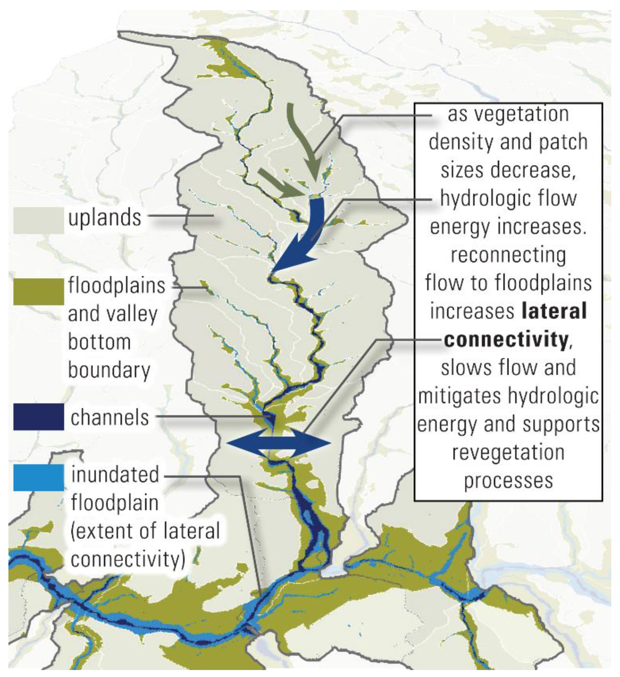
Figure 1. The dynamics of flood flow connections to the landscape are significant drivers of watershed conditions.
Systems 07 00053 g001
Figure 2. Managing the water budget targets the processes that connect water inputs into the storage functions and, thus, reveals the mechanisms for increasing water availability.
Systems 07 00053 g002
Figure 3. Outputs of the Flood Flow Connectivity to the Landscape (FlowCon) modeling framework that contributed to the generalizable and adaptable integrative socio-environmental system dynamics (SD) model addressed in this article. FlowCon identifies optimum locations and quantifies the resulting benefits and extent of management and collaborative support required for restoration of the critical landscape processes of reducing hydrologic energy through increasing water retention, recharge, and vegetative productivity. (a) Locations for reconnecting floodplains at varying priority levels; (b) effects on a synthetic hydrograph of executing the various levels. The top two priority levels were found to be the optimum levels for reversing degradation trends.
Systems 07 00053 g003
Figure 4. The project area typifies the water storage challenges faced across Southwestern landscapes. The Hatch and Mesilla Valleys, the largest areas of agricultural valleys along the New Mexican Rio Grande, rely upon snowpack to fill the reservoirs, which is becoming increasingly variable in its supply. The occurrences of droughts and a general increase in aridity are drying upland soils, decreasing vegetation, and resulting in scouring floods. Agriculture has the potential to manage these landscapes by slowing and spreading flood flow, which can recharge soil stocks and refill aquifers.
Systems 07 00053 g004
Figure 5. The upland section of the FlowCon SD model. See Figure 6 for the downstream valley section. The SD model includes both the existing system and the scenarios of spreading flood flow and storm water, which are indicated in the model by variable shapes filled with dark-orange and bold connectors.
Systems 07 00053 g005
Figure 6. The valley section of the FlowCon SD model to support farmers to increase water availability through recharge and stormwater spreading.
Systems 07 00053 g006
Figure 7. Precipitation input is a pink-noise random variation based upon a mean of 10.41 inches (264 mm)/year with a standard deviation of 1.8 inches (45.72 mm). (Note that a common standard in system dynamics models and employed in several graphs in this work is to characterize the behavior in a graph more clearly by not starting the y-axis at zero.)
Systems 07 00053 g007
Figure 8. Benefits realized by local land managers in the upland systems (a) and the valley systems (b). Three scenarios are shown in the results beginning in this Figure: “No interventions” which represents the base case scenario with no additional flow connectivity management, “Support 1—execution only” which represents outside financial support to execute the new practices on a wider scale quickly, and “Support 2—experimentation and execution” which represents additional support for a phase of experimentation for a better fit to the local conditions to realize productivity benefits more quickly and to a greater extent, which leads to a perception of greater legitimacy of the practices.
Systems 07 00053 g008
Figure 9. Surface spreading in the uplands (SSa) begins with an optimal target identified by the FlowCon framework for this system (which would be different in other systems) to reduce the runoff quantity by 35%, as that target correlates to sufficient reductions in the peak flows. SSa (a) reduces stormwater runoff (Qr) (b). Approximately 15% of the diverted flow on average is infiltrated and results in reduction of runoff; therefore, the initial targeted surface spreading is approximately 120,000 AF (Acre Feet), as is shown achieved by the Support 2 scenario (a). The reduction of 35% of Qr is also shown achieved by the Support 2 scenario (b).
Systems 07 00053 g009
Figure 10. This system is structured with a trend of modest groundwater declines to mimic likely site and common aquifer dynamics, as can be seen in the blue line and noting the fine scale of the y-axis starting at 19 million AF. While stormwater runoff (Qr) is substantially reduced, as shown in Figure 9, the combined intervention effects considered legitimate are still enough to quickly reverse the trend of shallow groundwater aquifer decline. While the differences might appear insignificant, typically only a ratio of the groundwater aquifer storage is usable and, as levels decline, the corresponding water quality generally also declines, decreasing that ratio. Each system would have different base conditions and different targets.
Systems 07 00053 g010
Figure 11. Stormwater (SW) out of the valley (Qout) is reduced in a scenarios resulting from management targets of reduction of higher-energy storm events that would carry sediment transport. The reduction does not impact the downstream compact allocation (Cd) quantity (679,000 AFY).
Systems 07 00053 g011
Figure 12. In the upland system, the additional infiltration in the floodplains of the valley bottoms results in additional vegetation coverage (VCa) (a). This in turn fuels surface spreading (SSa) which produces infiltration additional (AIup) (b) to the normal infiltration (Iu) in the valley (as shown in Figure 5).
Systems 07 00053 g012
Figure 13. The valley farmers’ production is directly related to water availability. Withdrawals (W) (a) increase with the stormwater spreading (SWa) interventions (c) reducing any surface water supply compact allocation gap (d) and thus the need for groundwater pumping (GWout) (b), known as “in-lieu recharge”. The recovery policy ratio (Rp) for farmers able to capture and reuse groundwater is 0.75. This resulting effect of increasing groundwater levels and storage benefits the valley farmers with greater water availability in the form of W. Both support scenarios shown in red and orange produce similar results.
Systems 07 00053 g013
Figure 14. The reference modes of behavior of productivity benefit uplands (PBu) (a) and productivity benefit valley (PBv) (b). For both figures, the support scenario 2 experimentation to fit the practice to the local conditions would yield productivity benefits more quickly and to a greater extent, leading to a perception of greater legitimacy of the practices. Additionally, it would provide local collaboration, which would lead to increased innovation and greater adoption. The support scenario 1 of outside support to simply shoulder the management burden would experience a longer learning curve and greater adaptive management inputs to correct unintended consequences, yielding slower and less robust benefit yields over time.
Systems 07 00053 g014
Figure 15. Compact allocations determine the distribution of surface water upstream from the system (a), and they are affected by upstream precipitation/snowpack variability (b), where any quantity below a mean set by the compact agreement diminishes the allocation.
Systems 07 00053 g015
Table 1. Boundary of the model. * indicates initial or exogenous value inputs from the other Flood Flow Connectivity to the Landscape (FlowCon) framework model outputs.
EndogenousExogenousExcluded
Main water balance variablesPractices that do not address the natural and social management systems, such as aquifer storage and recovery (injection wells)
Surface water*
(Qin, Qu, Qv)
Precipitation (Pm)
(Pr affected by pink noise random variability)
Soil moisture (SMup, SMv)Water compact agreements (Cl, Cd, Wr)
(actual amount varies with supply)
Groundwater* (GW)E and ET fractions (ETup, ETvr, Er) (upland varies within a range of 0.55 and 0.85; valley is 0.92)
Stormwater runoff (Qr)Infiltration * and conveyance efficiency fractions (Ifp, If, Ir, Lc)—from FlowCon
Critical scenario variables
Additional infiltration*
(AIup, AIv)
Downstream effects *,
e.g., in this site, effects on Texas and Mexico
(represented by two scenarios of S:
Support 1: S = 0, no support from downstream beneficiaries, and Support 2: S = 0.2, support from downstream beneficiaries)
Sediment transport or precipitation intensity measured directly (proxy is reduced stormwater runoff (Qr) in the quantities and character assessed to achieve this goal outside of this model)
Vegetation coverage* (VCa)
Benefits perceived legitimate
(BLu, BLv)
Surface spreading potential ratio targets *
(SSr = 0.2, SWSr = 1)
Benefit evaluation (Bu, Bv)Productivity benefits (PBu, PBv)
(see Figure 14 for the graphical functions)
Withdrawals change (Wc)Recovery policy ratio (Rp)