A System Dynamics Model Examining Alternative Wildfire Response Policies


Abstract
1. Introduction
1.1. Background and Overview
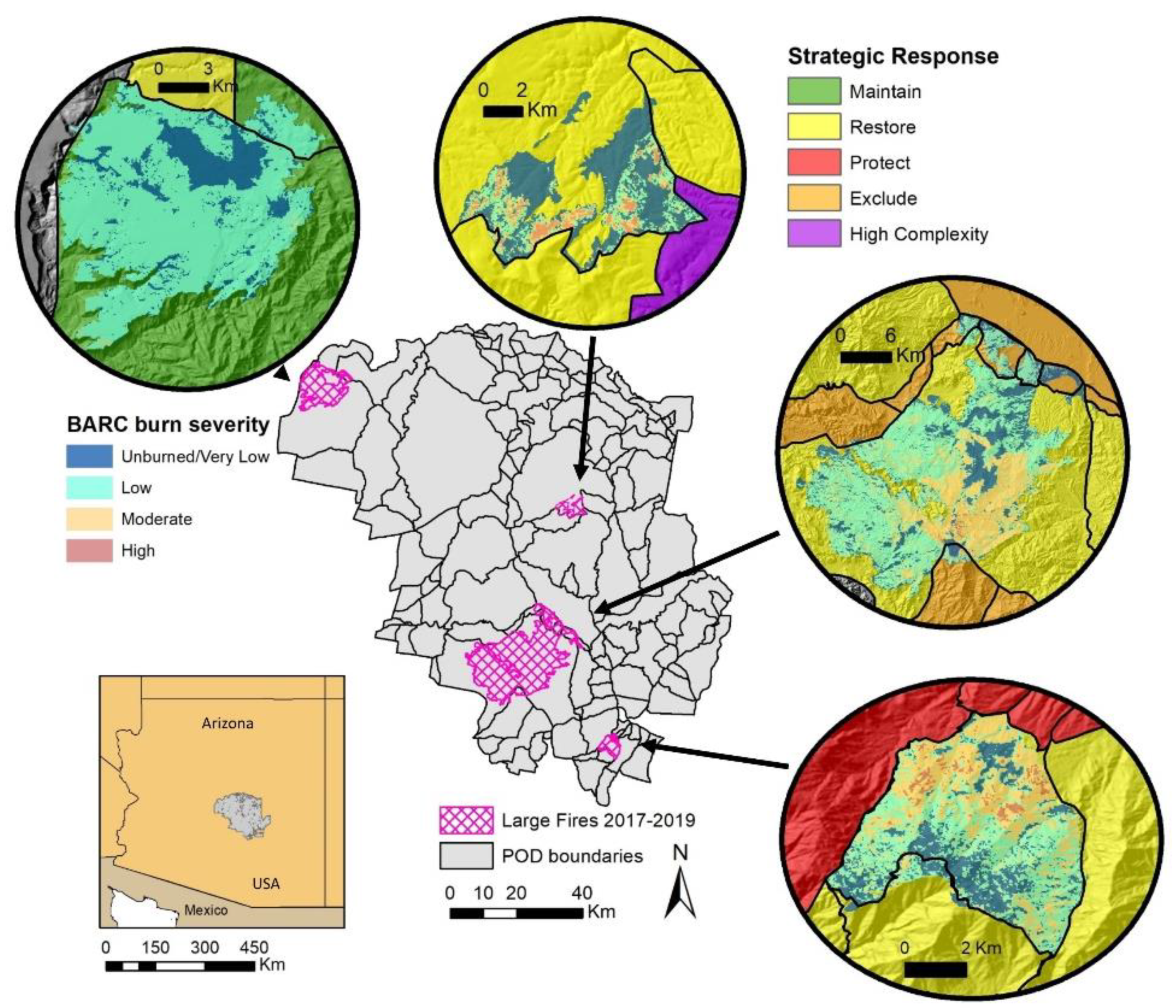
1.2. Management Context
2. Materials and Methods
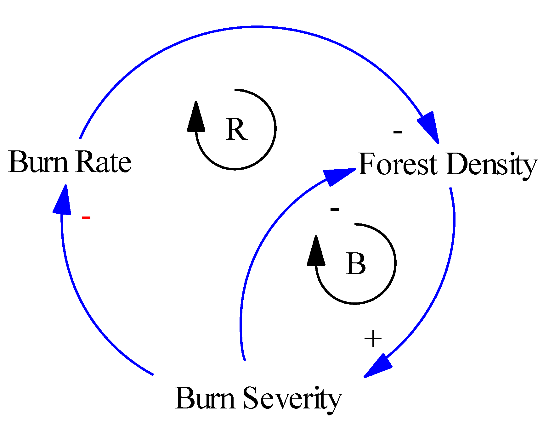
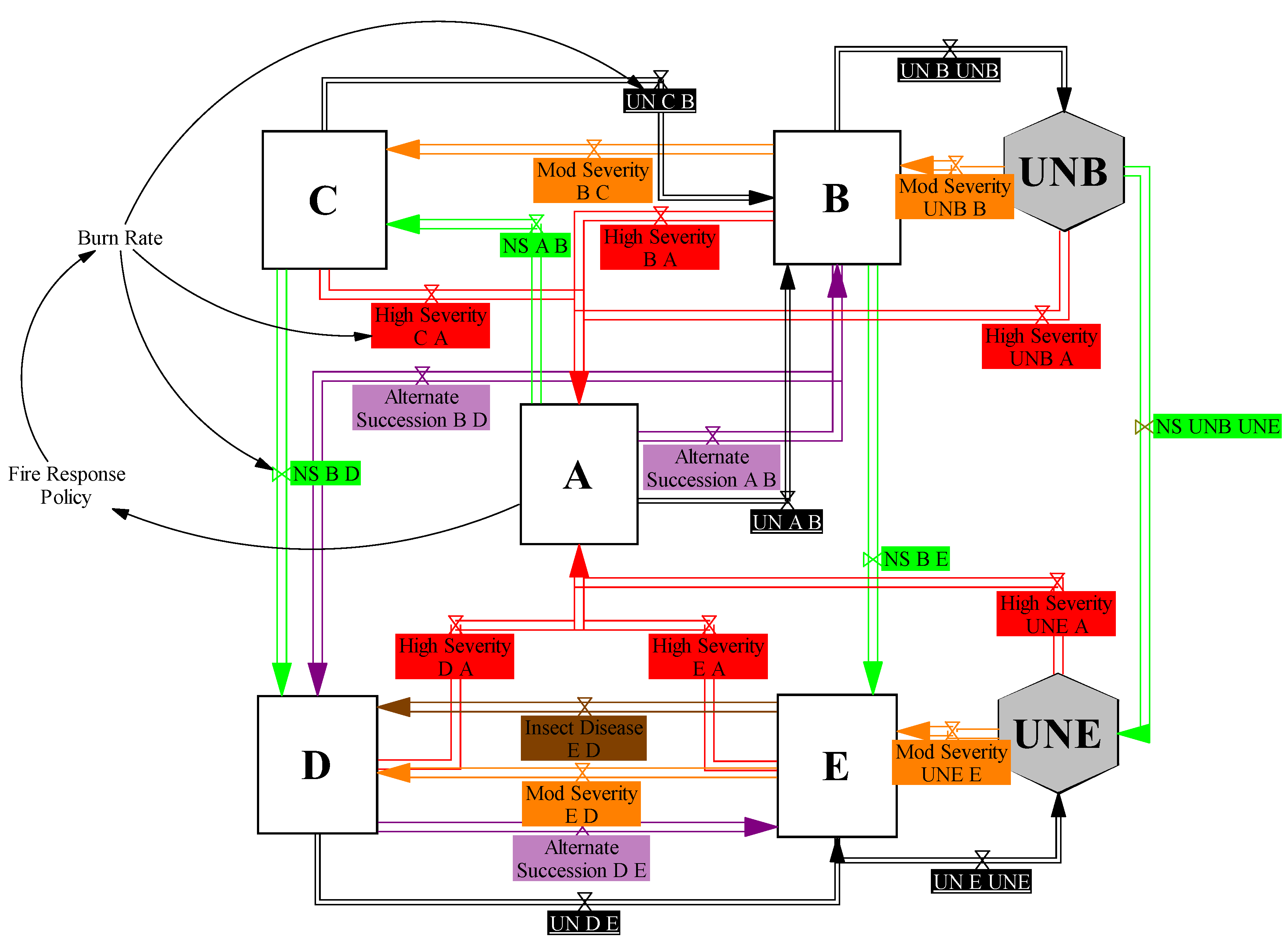
2.1. Model of Forest and Fire Dynamics
- index for S-Class i
- natural succession transition time (i.e., measured by years) for S-Class i
- burn rate (i.e., annual burn rate) for S-Class i
- user-defined fuel accumulation rate parameter for S-Class i. By setting , we would assume the S-Class i transfers into the corresponding UN class faster than the natural succession rate calculated as
2.2. Wildfire Response Policy Scenarios
3. Results
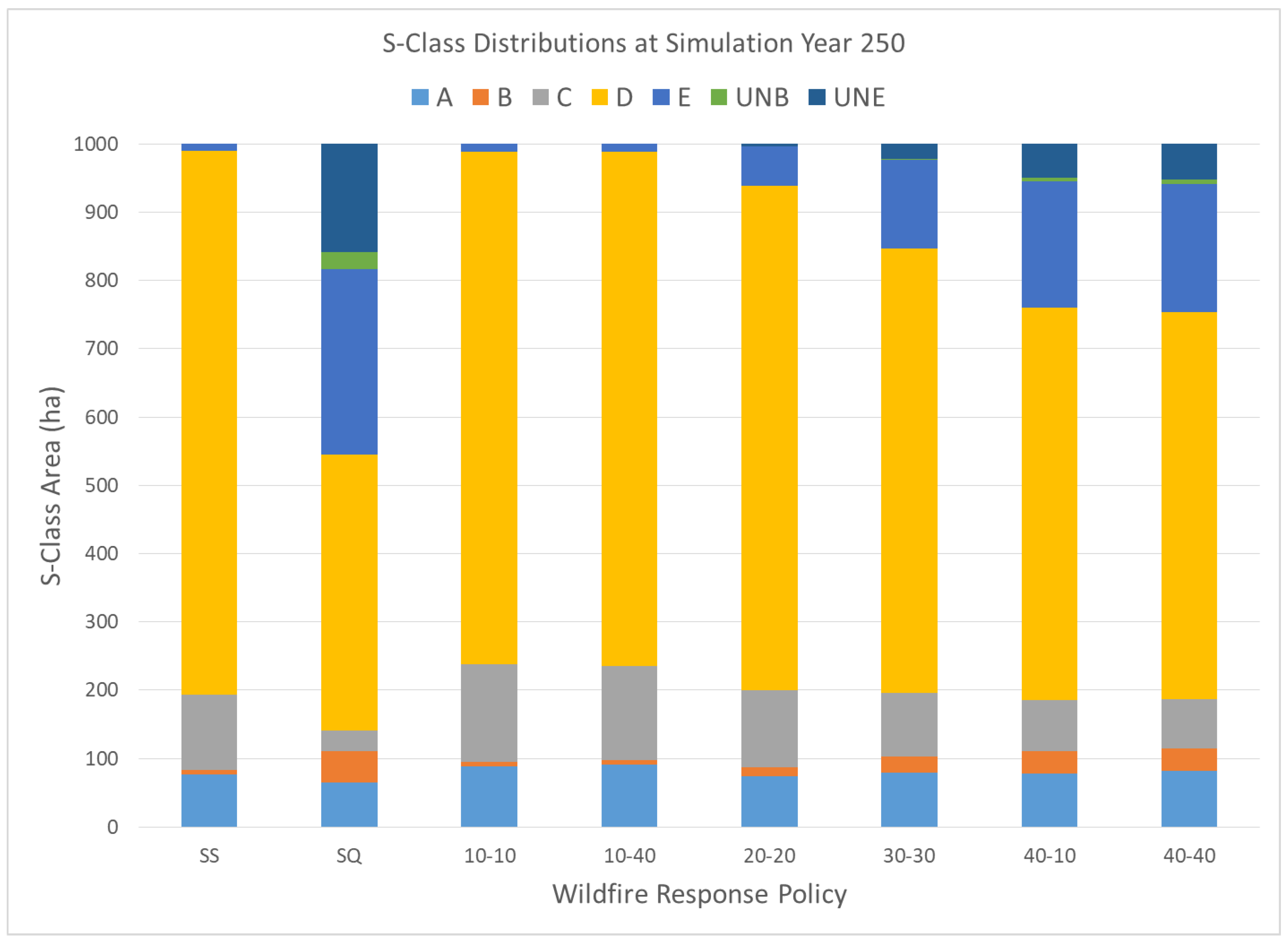
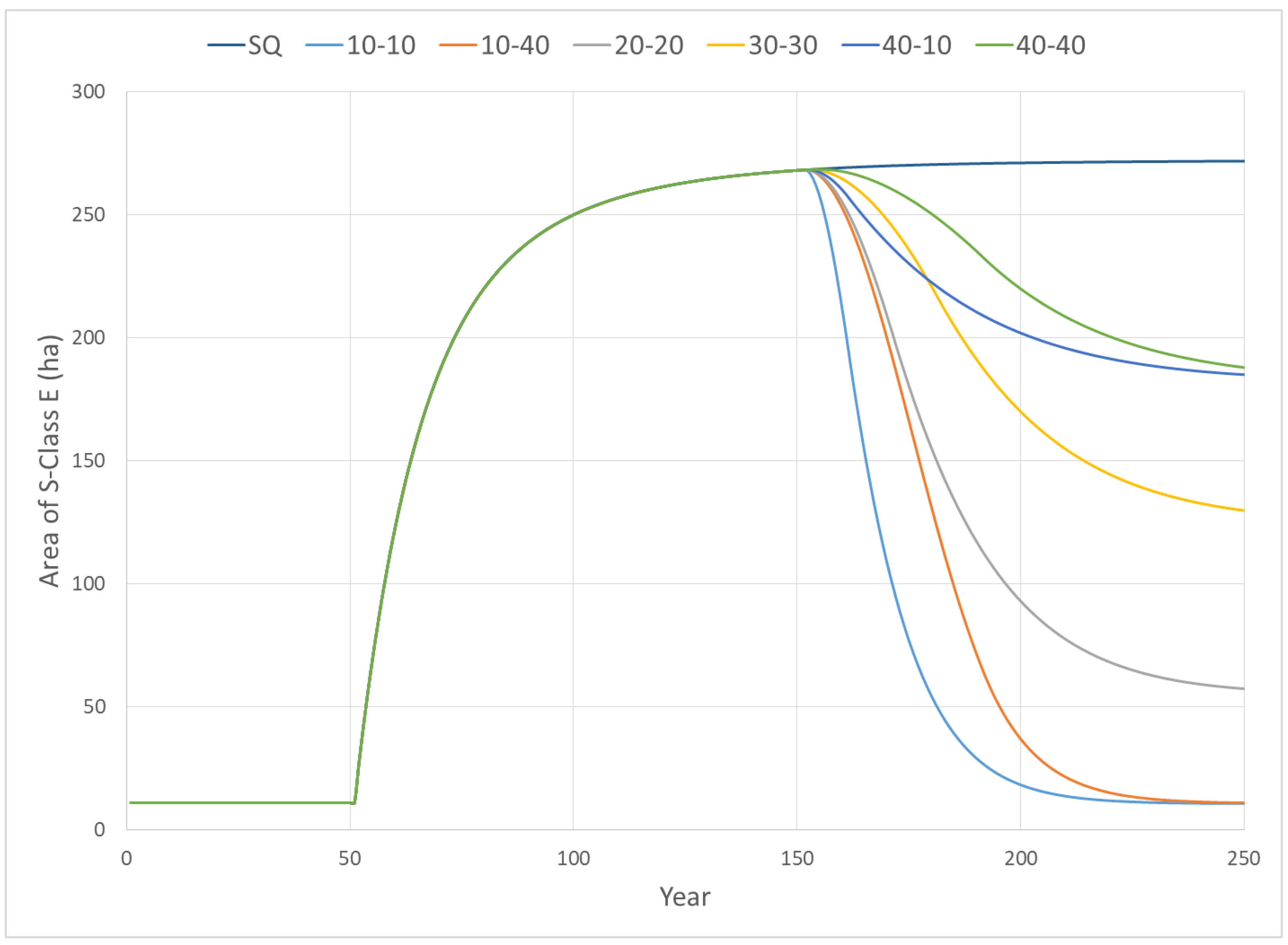
3.1. Policy Analysis
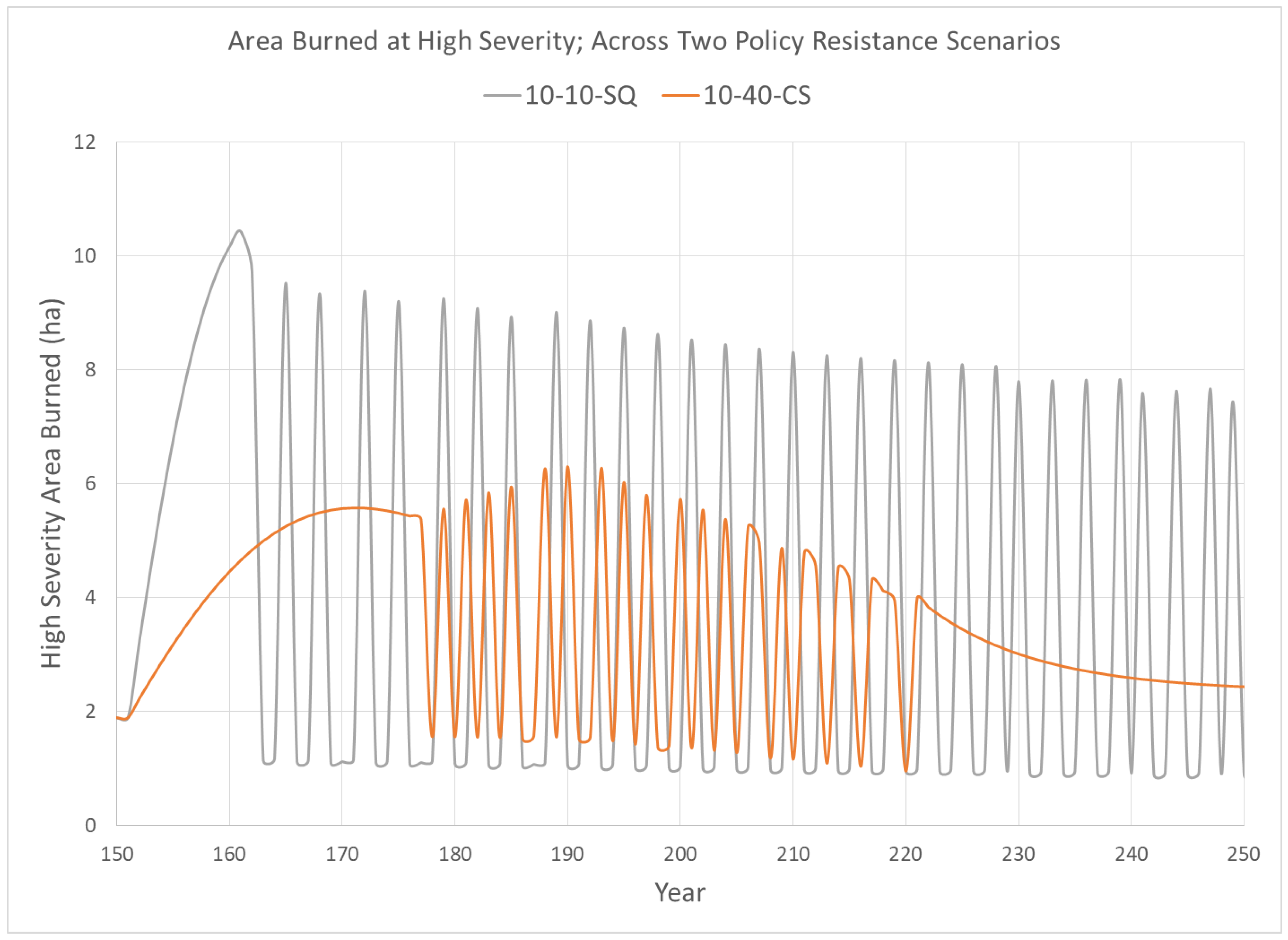
3.2. Policy Resistance
4. Discussion
4.1. Policy Insights and Management Recommendations
4.2. Limitations and Extensions
5. Conclusions
Author Contributions
Funding
Acknowledgments
Conflicts of Interest
Appendix A


References
- Steelman, T.; Nowell, B. Evidence of effectiveness in the Cohesive Strategy: Measuring and improving wildfire response. Int. J. Wildland Fire 2019, 28, 267–274. [Google Scholar] [CrossRef]
- Thompson, M.P.; Dunn, C.J.; Calkin, D.E. Systems thinking and wildland fire management. In Proceedings of the 60th Annual Meeting of the ISSS-2016, Boulder, CO, USA, 23–30 July 2016; Volume 1. No. 1. [Google Scholar]
- Thompson, M.P.; MacGregor, D.G.; Dunn, C.J.; Calkin, D.E.; Phipps, J. Rethinking the wildland fire management system. J. For. 2018, 116, 382–390. [Google Scholar] [CrossRef]
- Spies, T.A.; Hammer, R.; White, E.M.; Kline, J.D.; Bailey, J.; Bolte, J.; Platt, E.; Olsen, C.S.; Jacobs, D.; Shindler, B. Examining fire-prone forest landscapes as coupled human and natural systems. Ecol. Soc. 2014, 19, 9. [Google Scholar] [CrossRef]
- Calkin, D.E.; Thompson, M.P.; Finney, M.A. Negative consequences of positive feedbacks in US wildfire management. For. Ecosyst. 2015, 2, 9. [Google Scholar] [CrossRef]
- North, M.P.; Stephens, S.L.; Collins, B.M.; Agee, J.K.; Aplet, G.; Franklin, J.F.; Fule, P.Z. Reform forest fire management. Science 2015, 349, 1280–1281. [Google Scholar] [CrossRef]
- Parks, S.A.; Holsinger, L.M.; Miller, C.; Nelson, C.R. Wildland fire as a self-regulating mechanism: The role of previous burns and weather in limiting fire progression. Ecol. Appl. 2015, 25, 1478–1492. [Google Scholar] [CrossRef]
- Regos, A.; Aquilué, N.; Retana, J.; De Cáceres, M.; Brotons, L. Using unplanned fires to help suppressing future large fires in Mediterranean forests. PLoS ONE 2014, 9, e94906. [Google Scholar] [CrossRef]
- Thompson, M.P.; Freeborn, P.; Rieck, J.D.; Calkin, D.E.; Gilbertson-Day, J.W.; Cochrane, M.A.; Hand, M.S. Quantifying the influence of previously burned areas on suppression effectiveness and avoided exposure: A case study of the Las Conchas Fire. Int. J. Wildland Fire 2016, 25, 167–181. [Google Scholar] [CrossRef]
- North, M.; Brough, A.; Long, J.; Collins, B.; Bowden, P.; Yasuda, D.; Miller, J.; Sugihara, N. Constraints on mechanized treatment significantly limit mechanical fuels reduction extent in the Sierra Nevada. J. For. 2014, 113, 40–48. [Google Scholar] [CrossRef]
- Barnett, K.; Parks, S.; Miller, C.; Naughton, H. Beyond fuel treatment effectiveness: Characterizing Interactions between fire and treatments in the US. Forests 2016, 7, 237. [Google Scholar] [CrossRef]
- Vaillant, N.M.; Reinhardt, E.D. An evaluation of the Forest Service Hazardous Fuels Treatment Program—Are we treating enough to promote resiliency or reduce hazard? J. For. 2017, 115, 300–308. [Google Scholar] [CrossRef]
- Schultz, C.; Huber-Stearns, H.; McCaffrey, S.; Quirke, D.; Ricco, G.; Moseley, C. Prescribed Fire Policy Barriers and Opportunities: A Diversity of Challenges and Strategies Across the West; Ecosystem Workforce Program Institute for a Sustainable Environment, University of Oregon: Eugene, OR, USA, 2018; Available online: https://ewp.uoregon.edu/sites/ewp.uoregon.edu/files/WP_86.pdf (accessed on 10 July 2019).
- North, M.; Collins, B.M.; Stephens, S. Using fire to increase the scale, benefits, and future maintenance of fuels treatments. J. For. 2012, 110, 392–401. [Google Scholar] [CrossRef]
- Collins, B.M.; Lydersen, J.M.; Fry, D.L.; Wilkin, K.; Moody, T.; Stephens, S.L. Variability in vegetation and surface fuels across mixed-conifer-dominated landscapes with over 40 years of natural fire. For. Ecol. Manag. 2016, 381, 74–83. [Google Scholar] [CrossRef]
- Boisramé, G.F.; Thompson, S.E.; Kelly, M.; Cavalli, J.; Wilkin, K.M.; Stephens, S.L. Vegetation change during 40 years of repeated managed wildfires in the Sierra Nevada, California. For. Ecol. Manag. 2017, 402, 241–252. [Google Scholar]
- Boisramé, G.; Thompson, S.; Collins, B.; Stephens, S. Managed wildfire effects on forest resilience and water in the Sierra Nevada. Ecosystems 2017, 20, 717–732. [Google Scholar]
- Haugo, R.D.; Kellogg, B.S.; Cansler, C.A.; Kolden, C.A.; Kemp, K.B.; Robertson, J.C.; Metlen, K.L.; Vaillant, N.M.; Restaino, C.M. The missing fire: Quantifying human exclusion of wildfire in Pacific Northwest forests, USA. Ecosphere 2019, 10, e02702. [Google Scholar] [CrossRef]
- Houtman, R.M.; Montgomery, C.A.; Gagnon, A.R.; Calkin, D.E.; Dietterich, T.G.; McGregor, S.; Crowley, M. Allowing a wildfire to burn: Estimating the effect on future fire suppression costs. Int. J. Wildland Fire 2013, 22, 871–882. [Google Scholar] [CrossRef]
- Barros, A.M.; Ager, A.A.; Day, M.A.; Krawchuk, M.A.; Spies, T.A. Wildfires managed for restoration enhance ecological resilience. Ecosphere 2018, 9, e02161. [Google Scholar] [CrossRef]
- Taylor, M.H.; Sanchez Meador, A.J.; Kim, Y.S.; Rollins, K.; Will, H. The economics of ecological restoration and hazardous fuel reduction treatments in the ponderosa pine forest ecosystem. For. Sci. 2015, 61, 988–1008. [Google Scholar] [CrossRef]
- Keane, R.E.; Gray, K.; Davis, B.; Holsinger, L.M.; Loehman, R. Evaluating ecological resilience across wildfire suppression levels under climate and fuel treatment scenarios using landscape simulation modelling. Int. J. Wildland Fire 2019, 28, 533–549. [Google Scholar] [CrossRef]
- Riley, K.; Thompson, M.; Scott, J.; Gilbertson-Day, J. A model-based framework to evaluate alternative wildfire suppression strategies. Resources 2018, 7, 4. [Google Scholar] [CrossRef]
- Collins, R.D.; de Neufville, R.; Claro, J.; Oliveira, T.; Pacheco, A.P. Forest fire management to avoid unintended consequences: A case study of Portugal using system dynamics. J. Environ. Manag. 2013, 130, 1–9. [Google Scholar] [CrossRef] [PubMed]
- O’Connor, C.; Thompson, M.; Rodríguez y Silva, F. Getting ahead of the wildfire problem: Quantifying and mapping management challenges and opportunities. Geosciences 2016, 6, 35. [Google Scholar] [CrossRef]
- O’Connor, C.D.; Calkin, D.E.; Thompson, M.P. An empirical machine learning method for predicting potential fire control locations for pre-fire planning and operational fire management. Int. J. Wildland Fire 2017, 26, 587–597. [Google Scholar]
- Wei, Y.; Thompson, M.P.; Scott, J.H.; O’Connor, C.D.; Dunn, C.J. Designing Operationally Relevant Daily Large Fire Containment Strategies Using Risk Assessment Results. Forests 2019, 10, 311. [Google Scholar] [CrossRef]
- Ingalsbee, T. Whither the paradigm shift? Large wildland fires and the wildfire paradox offer opportunities for a new paradigm of ecological fire management. Int. J. Wildland Fire 2017, 26, 557–561. [Google Scholar] [CrossRef]
- DeMeo, T.; Haugo, R.; Ringo, C.; Kertis, J.; Acker, S.; Simpson, M.; Stern, M. Expanding Our Understanding of Forest Structural Restoration Needs in the Pacific Northwest. Northwest Sci. 2018, 92, 18–36. [Google Scholar] [CrossRef]
- Scott, J.H.; Helmbrecht, D.J.; Thompson, M.P. Assessing the Expected Effects of Wildfire on Vegetation Condition on the Bridger-Teton National Forest, Wyoming, USA; Res. Note: RMRS-RN-7; US Department of Agriculture, Forest Service, Rocky Mountain Research Station: Fort Collins, CO, USA, 2014; Volume 71, p. 36.
- Minas, J.P.; Hearne, J.W.; Handmer, J.W. A review of operations research methods applicable to wildfire management. Int. J. Wildland Fire 2012, 21, 189–196. [Google Scholar] [CrossRef]
- Martell, D.L. A review of recent forest and wildland fire management decision support systems research. Curr. For. Rep. 2015, 1, 128–137. [Google Scholar] [CrossRef]
- Littell, J.S.; McKenzie, D.; Peterson, D.L.; Westerling, A.L. Climate and wildfire area burned in western US ecoprovinces, 1916–2003. Ecol. Appl. 2009, 19, 1003–1021. [Google Scholar] [CrossRef]
- Parks, S.; Dobrowski, S.; Panunto, M. What Drives Low-Severity Fire in the Southwestern USA? Forests 2018, 9, 165. [Google Scholar] [CrossRef]
- O’Connor, C.D.; Falk, D.A.; Lynch, A.M.; Swetnam, T.W.; Wilcox, C.P. Disturbance and productivity interactions mediate stability of forest composition and structure. Ecol. Appl. 2017, 27, 900–915. [Google Scholar] [CrossRef] [PubMed]
- Barros, A.M.; Ager, A.A.; Day, M.A.; Palaiologou, P. Improving long-term fuel treatment effectiveness in the National Forest System through quantitative prioritization. For. Ecol. Manag. 2019, 433, 514–527. [Google Scholar] [CrossRef]
- Finney, M.A.; Seli, R.C.; McHugh, C.W.; Ager, A.A.; Bahro, B.; Agee, J.K. Simulation of long-term landscape-level fuel treatment effects on large wildfires. Int. J. Wildland Fire 2008, 16, 712–727. [Google Scholar] [CrossRef]
- Scott, J.H.; Thompson, M.P.; Gilbertson-Day, J.W. Examining alternative fuel management strategies and the relative contribution of National Forest System land to wildfire risk to adjacent homes—A pilot assessment on the Sierra National Forest, California, USA. For. Ecol. Manag. 2016, 362, 29–37. [Google Scholar] [CrossRef]
- Gannon, B.M.; Wei, Y.; MacDonald, L.H.; Kampf, S.K.; Jones, K.W.; Cannon, J.B.; Wolk, B.H.; Cheng, A.S.; Addington, R.N.; Thompson, M.P. Prioritising fuels reduction for water supply protection. Int. J. Wildland Fire 2019. [Google Scholar] [CrossRef]
- Fire Executive Council. Guidance for Implementation of Federal Wildland Fire Management Policy. 2009. Available online: https://www.nifc.gov/policies/policies_documents/GIFWFMP.pdf (accessed on 22 July 2019).
- National Interagency Fire Center. Interagency Standards for Fire and Fire Aviation Operations 2019. 2019. Available online: https://www.nifc.gov/policies/pol_ref_redbook.html (accessed on 22 July 2019).
- Thompson, M.; Bowden, P.; Brough, A.; Scott, J.; Gilbertson-Day, J.; Taylor, A.; Anderson, J.; Haas, J. Application of wildfire risk assessment results to wildfire response planning in the southern Sierra Nevada, California, USA. Forests 2016, 7, 64. [Google Scholar] [CrossRef]
- O’Connor, C.D.; Calkin, D.E. Engaging the fire before it starts: A case study from the 2017 Pinal Fire (Arizona). Wildfire 2019, 28, 14–18. [Google Scholar]
- Dunn, C.J.; Thompson, M.P.; Calkin, D.E. A framework for developing safe and effective large-fire response in a new fire management paradigm. For. Ecol. Manag. 2017, 404, 184–196. [Google Scholar] [CrossRef]
- Meadows, D. Thinking in Systems: A Primer; Chelsea Green Publishing: White River Junction, VT, USA, 2008. [Google Scholar]
- Fischer, A.P.; Spies, T.A.; Steelman, T.A.; Moseley, C.; Johnson, B.R.; Bailey, J.D.; Ager, A.A.; Bourgeron, P.; Charnley, S.; Collins, B.M.; et al. Wildfire risk as a socioecological pathology. Front. Ecol. Environ. 2016, 14, 276–284. [Google Scholar] [CrossRef]
- Hamilton, M.; Fischer, A.P.; Ager, A. A social-ecological network approach for understanding wildfire risk governance. Glob. Environ. Chang. 2019, 54, 113–123. [Google Scholar] [CrossRef]
- Paveglio, T.B.; Moseley, C.; Carroll, M.S.; Williams, D.R.; Davis, E.J.; Fischer, A.P. Categorizing the social context of the wildland urban interface: Adaptive capacity for wildfire and community “archetypes”. For. Sci. 2014, 61, 298–310. [Google Scholar] [CrossRef]
- Rollins, M.G. LANDFIRE: A nationally consistent vegetation, wildland fire, and fuel assessment. Int. J. Wildland Fire 2009, 18, 235–249. [Google Scholar] [CrossRef]
- Ryan, K.C.; Opperman, T.S. LANDFIRE—A national vegetation/fuels data base for use in fuels treatment, restoration, and suppression planning. For. Ecol. Manag. 2013, 294, 208–216. [Google Scholar] [CrossRef]
- Tedim, F.; Leone, V.; Amraoui, M.; Bouillon, C.; Coughlan, M.; Delogu, G.; Fernandes, P.; Ferreira, C.; McCaffrey, S.; McGee, T.; et al. Defining extreme wildfire events: Difficulties, challenges, and impacts. Fire 2018, 1, 9. [Google Scholar] [CrossRef]
- Stevens, J.T.; Collins, B.M.; Miller, J.D.; North, M.P.; Stephens, S.L. Changing spatial patterns of stand-replacing fire in California conifer forests. For. Ecol. Manag. 2017, 406, 28–36. [Google Scholar] [CrossRef]
- Page, W.G.; Alexander, M.E.; Jenkins, M.J. Wildfire’s resistance to control in mountain pine beetle-attacked lodgepole pine forests. For. Chron. 2013, 89, 783–794. [Google Scholar] [CrossRef]
- Dunn, C.J.; O’Connor, C.D.; Reilly, M.J.; Calkin, D.E.; Thompson, M.P. Spatial and temporal assessment of responder exposure to snag hazards in post-fire environments. For. Ecol. Manag. 2019, 441, 202–214. [Google Scholar] [CrossRef]
- Daniel, C.J.; Frid, L.; Sleeter, B.M.; Fortin, M.J. State-and-transition simulation models: A framework for forecasting landscape change. Methods Ecol. Evol. 2016, 7, 1413–1423. [Google Scholar] [CrossRef]
- Hart, S.J.; Henkelman, J.; McLoughlin, P.D.; Nielsen, S.E.; Truchon-Savard, A.; Johnstone, J.F. Examining forest resilience to changing fire frequency in a fire-prone region of boreal forest. Glob. Chang. Biol. 2019, 25, 869–884. [Google Scholar] [CrossRef]
- Wei, Y.; Thompson, M.P.; Haas, J.R.; Dillon, G.K.; O’Connor, C.D. Spatial optimization of operationally relevant large fire confine and point protection strategies: Model development and test cases. Can. J. For. Res. 2018, 48, 480–493. [Google Scholar] [CrossRef]
- Stevens-Rumann, C.S.; Kemp, K.B.; Higuera, P.E.; Harvey, B.J.; Rother, M.T.; Donato, D.C.; Morgan, P.; Veblen, T.T. Evidence for declining forest resilience to wildfires under climate change. Ecol. Lett. 2018, 21, 243–252. [Google Scholar] [CrossRef] [PubMed]
| 1 | Hereafter when we refer to “policy scenarios” we do not mean changing Federal Policy but rather localized changes in response to wildfires. |


| Label | Name | Description |
|---|---|---|
| A | Early Development—All Structures | Openings with grass, shrubs, and forbs created after replacement fire |
| B | Mid Development—Closed | Closed pole-sapling/grass and shrubs, with tree heights of 0–10 m and forest canopy closure > 30% |
| C | Mid Development—Open | Open pole-sapling/grass and shrubs with tree heights 0–10 m and forest canopy closure < 30% |
| D | Late Development—Open | Open large trees/grass and shrubs with tree heights > 10 m and canopy cover between 30–60% |
| E | Late Development—Closed | Closed large trees, poles, saplings, and shrubs with tree heights > 10 m and forest canopy cover between 30–60% |
| UN-B | Mid Development—Uncharacteristic | Uncharacteristic closed mid-development with forest canopy cover > 60% |
| UN-E | Late Development—Uncharacteristic | Uncharacteristic closed late-development with forest canopy cover > 60% |
| Upper Layer Lifeform | Height (m) | Canopy Cover | |||||||||
|---|---|---|---|---|---|---|---|---|---|---|---|
| 0–10 | 11–20 | 21–30 | 31–40 | 41–50 | 51–60 | 61–70 | 71–80 | 81–90 | 91–100 | ||
| Herb | 0–0.5 | A | A | A | A | A | A | A | A | A | A |
| Herb | 0.5–1.0 | A | A | A | A | A | A | A | A | A | A |
| Herb | >1.0 | A | A | A | A | A | A | A | A | A | A |
| Shrub | 0–0.5 | A | A | A | A | A | A | A | A | A | A |
| Shrub | 0.5–1.0 | A | A | A | A | A | A | A | A | A | A |
| Shrub | 1.0–3.0 | A | A | A | A | A | A | A | A | A | A |
| Shrub | >3.0 | A | A | A | A | A | A | A | A | A | A |
| Tree | 0-5 | C | C | C | B | B | B | UNB | UNB | UNB | UNB |
| Tree | 5–10 | C | C | C | B | B | B | UNB | UNB | UNB | UNB |
| Tree | 10–25 | D | D | D | E | E | E | UNE | UNE | UNE | UNE |
| Tree | 25–50 | D | D | D | E | E | E | UNE | UNE | UNE | UNE |
| Tree | >50 | D | D | D | E | E | E | UNE | UNE | UNE | UNE |
| From S-Class | To S-Class | Flow Type | Flow Rate Determinants | Flow Rate |
|---|---|---|---|---|
| A | A | Low-Severity Fire | Conditional Probability | BRA × 1.00 |
| A | B | Alternative Succession | - | 0.01 |
| A | B | UN | TA = 50 | Equation (1) |
| A | C | NS | TA = 50 | Equation (2) |
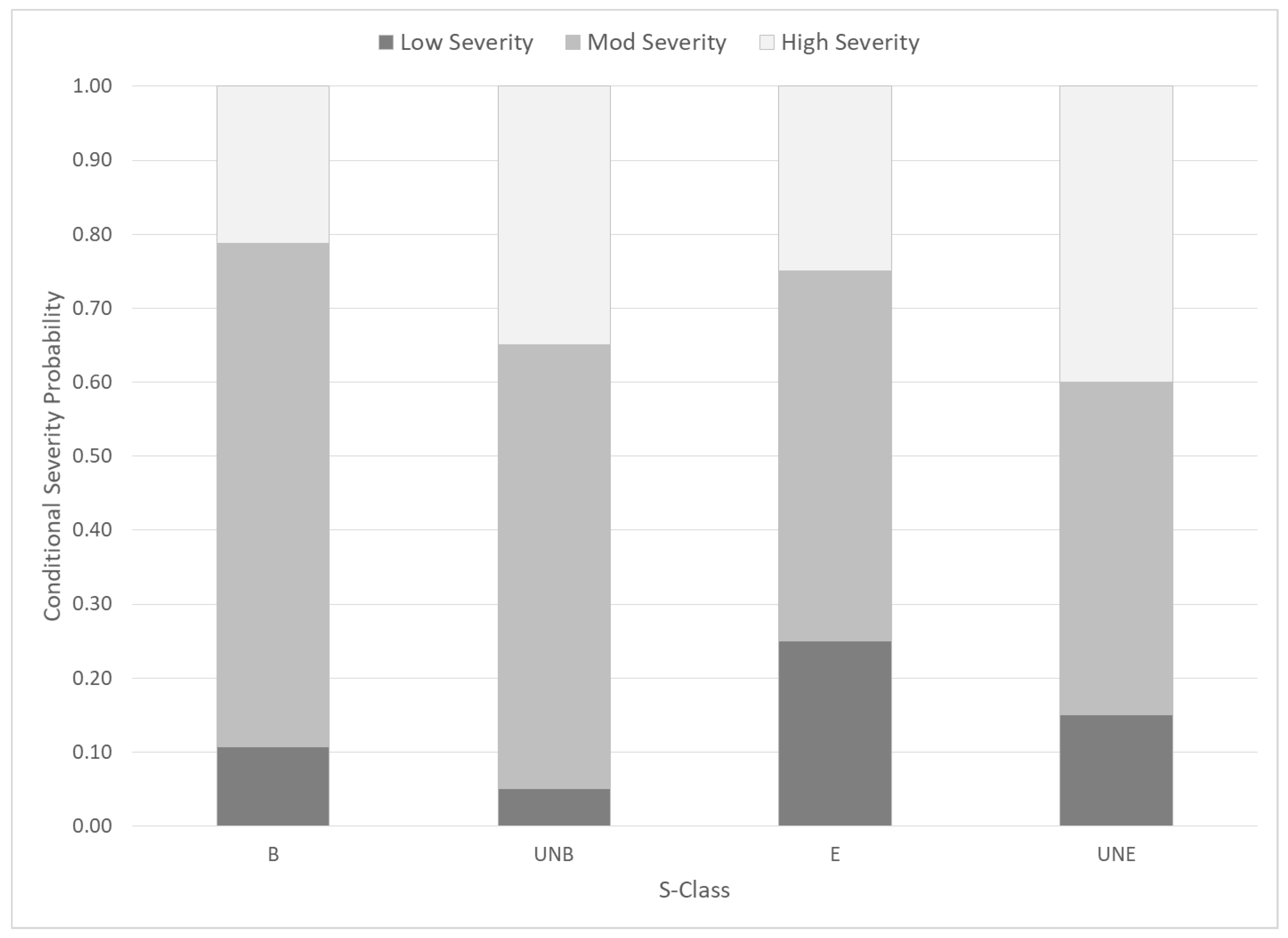
| B | A | High-Severity Fire | Conditional Probability | BRB * 0.21 |
| B | B | Low-Severity Fire | Conditional Probability | BRB * 0.11 |
| B | C | Moderate-Severity Fire | Conditional Probability | BRB * 0.68 |
| B | D | Alternative Succession | - | 0.03 |
| B | E | NS | TB = 70 | Equation (2) |
| B | UNB | UN | TB = 70 | Equation (1) |
| C | A | High-Severity Fire | Conditional Probability | BRC * 0.03 |
| C | B | UN | TC = 70 | Equation (1) |
| C | C | Low-Severity Fire | Conditional Probability | BRC * 0.88 |
| C | C | Moderate-Severity Fire | Conditional Probability | BRC * 0.09 |
| C | D | NS | TC = 70 | Equation (2) |
| D | A | High-Severity Fire | Conditional Probability | BRD * 0.02 |
| D | D | Low-Severity Fire | Conditional Probability | BRD * 0.89 |
| D | D | Moderate-Severity Fire | Conditional Probability | BRD * 0.09 |
| D | E | Alternative Succession | - | 0.001 |
| D | E | UN | TD = 50 | Equation (1) |
| E | A | High-Severity Fire | Conditional Probability | BRE * 0.25 |
| E | D | Moderate-Severity Fire | Conditional Probability | BRE * 0.50 |
| E | D | Insect/Disease | - | 0.02 |
| E | E | Low-Severity Fire | Conditional Probability | BRE * 0.25 |
| E | UNE | UN | TE = 50 | Equation (1) |
| UNB | A | High-Severity Fire | Conditional Probability | BRUNB * 0.35 |
| UNB | B | Moderate-Severity Fire | Conditional Probability | BRUNB * 0.60 |
| UNB | UNB | Low-Severity Fire | Conditional Probability | BRUNB * 0.05 |
| UNB | UNE | NS | TUNB = 70 | Equation (2) |
| UNE | A | High-Severity Fire | Conditional Probability | BRUNE * 0.40 |
| UNE | E | Moderate-Severity Fire | Conditional Probability | BRUNE * 0.45 |
| UNE | UNE | Low-Severity Fire | Conditional Probability | BRUNE * 0.15 |
| Policy Label | Policy Description | Target Mean Fire Return Interval (Years) | Target Attainment Time (Years) |
|---|---|---|---|
| SQ | Status Quo | 80 | 1 |
| 10-10 | Hot and Fast | 10 | 10 |
| 10-40 | Hot and Slow | 10 | 40 |
| 20-20 | Partially Hot and Fast | 20 | 20 |
| 30-30 | Partially Cool and Slow | 30 | 30 |
| 40-10 | Cool and Fast | 40 | 10 |
| 40-40 | Cool and Slow | 40 | 40 |
| Policy Label | Policy Description | Target Mean Fire Return Interval (Years) | Target Attainment Time (Years) |
|---|---|---|---|
| 10-10-CS | Hot and Fast, then Cool and Slow | 10 (40) | 10 (40) |
| 10-10-SQ | Hot and Fast, then Status Quo | 10 (80) | 10 (1) |
| 10-40-CS | Hot and Slow, then Cool and Slow | 10 (40) | 40 (40) |
| 10-40-SQ | Hot and Slow, then Status Quo | 10 (80) | 40 (1) |
| Fire Management Policy | Time to Restore D (Years) | Time to Restore E (Years) | Mean Departure (ha) | Mean UNE (ha) | Mean Percent High Severity Fire | Mean High-Severity Fire (ha) |
|---|---|---|---|---|---|---|
| SQ | n/a | n/a | 954.54 | 153.93 | 15.62 | 1.95 |
| 10-10 | 12 | 52 | 270.41 | 19.67 | 4.36 | 3.68 |
| 10-40 | 20 | 69 | 328.75 | 32.18 | 5.60 | 3.45 |
| 20-20 | 22 | >100 | 381.36 | 39.14 | 6.85 | 2.87 |
| 30-30 | 36 | >100 | 567.42 | 65.94 | 9.53 | 2.71 |
| 40-10 | 46 | >100 | 650.16 | 79.15 | 10.78 | 2.59 |
| 40-40 | 64 | >100 | 715.80 | 94.35 | 11.77 | 2.57 |
| Fire Management Policy and Resistance Scenario | Time to Restore D (Years) | Time to Restore E (Years) | Mean Departure (ha) | Mean UNE (ha) | Mean Percent High-Severity Fire | Mean High-Severity Fire (ha) |
|---|---|---|---|---|---|---|
| 10-10-CS | 12 | >100 | 428.20 | 35.09 | 6.71 | 3.78 |
| 10-10-SQ | 48 | >100 | 580.85 | 51.36 | 8.77 | 3.88 |
| 10-40-CS | 20 | 97 | 396.58 | 37.13 | 6.53 | 3.54 |
| 10-40-SQ | 20 | >100 | 517.35 | 46.57 | 8.09 | 3.75 |
© 2019 by the authors. Licensee MDPI, Basel, Switzerland. This article is an open access article distributed under the terms and conditions of the Creative Commons Attribution (CC BY) license (http://creativecommons.org/licenses/by/4.0/).
Share and Cite
Thompson, M.P.; Wei, Y.; Dunn, C.J.; O’Connor, C.D. A System Dynamics Model Examining Alternative Wildfire Response Policies. Systems 2019, 7, 49. https://doi.org/10.3390/systems7040049
Thompson MP, Wei Y, Dunn CJ, O’Connor CD. A System Dynamics Model Examining Alternative Wildfire Response Policies. Systems. 2019; 7(4):49. https://doi.org/10.3390/systems7040049
Chicago/Turabian StyleThompson, Matthew P., Yu Wei, Christopher J. Dunn, and Christopher D. O’Connor. 2019. "A System Dynamics Model Examining Alternative Wildfire Response Policies" Systems 7, no. 4: 49. https://doi.org/10.3390/systems7040049
APA StyleThompson, M. P., Wei, Y., Dunn, C. J., & O’Connor, C. D. (2019). A System Dynamics Model Examining Alternative Wildfire Response Policies. Systems, 7(4), 49. https://doi.org/10.3390/systems7040049