Article

Adding Feedbacks and Non-Linearity to the Neoclassical Growth Model: A New Realm for System Dynamics Applications

Faculty and Informatics and Management, University of Hradec Králové, Rokitanského 62, 500 03 Hradec Králové, Czech Republic
*
Author to whom correspondence should be addressed.
Submission received: 17 January 2018 / Revised: 20 March 2018 / Accepted: 22 March 2018 / Published: 29 March 2018
(This article belongs to the Special Issue Modelling of Economic Systems)

Abstract

:
Modelling of economic systems is traditionally associated with a mathematical formalism that has its drawbacks and limitations. This study applies system dynamics as a specific modelling technique that enables us to modify and elaborate existing economic models and improve them both from a theoretical perspective and for practical applications. More specifically, the Solow-Swan growth model is enriched by feedback and non-linearity based on its extension by the energy sector. The influence and role of renewable resources are considered in this enhancement. The developed model is tested in two different scenarios and utilizes sensitivity analysis as the primary tool. Acquired outcomes offer a new perspective on the economy–energy nexus based on real data and demonstrate that system dynamics can be successfully used as a modelling tool even in the theoretical economics as a traditional discipline.

1. Introduction

Studies focused on the interrelationships of economic systems and environments have been a subject of interest for many decades. However, prevention of undesired global climate change, natural disasters, ocean garbage, and rising energy scarcity represent the most significant challenges currently facing humanity [1,2,3]. Their urgency has intensified and related research and modelling must endeavour to further assess levels quantitatively and qualitatively. The necessity of improved ways of coping with current environmental issues catalysed the emergence of new concepts, improvements to obsolete models, or reconsideration and re-evaluation of the existing body of knowledge. The establishment of the so-called circular economy can serve as an example. Urbinati, Chiaroni and Chiesa [4] emphasise that the Circular Economy paradigm has become a topic of debate concerning new and more sustainable industrial strategies and paradigms [5,6]. The Circular Economy aims at a significant change in the way we use our resources. This should be grounded on minimisation of existing open production systems (associated with a linear consumption model in which materials are obtained, used in production in order to create products and eventually become waste) and their substitution by closed production systems (based on the idea that resources are reused and remain in a loop of production and usage, allowing us to create additional value for a longer period [7]). The main streams of research dealing with this topic are [4]:
  • Industrial ecology—focuses on the establishment and development of eco-industrial networks as a way to apply the principles of Circular Economy in practice [8].
  • Environmental, political, and social science—looks at the new industrial paradigm as a way to encourage people toward more sustainable behaviours or as a tool for policymakers to develop Circular Economy-driven environmental and management policies including new regulations that incorporate principles of sustainability [9] or [10].
  • Product design practices—looks at the Circular Economy paradigm by emphasizing the pivotal role played by the activities of design for recycling, design for remanufacturing and reuse, design for disassembly and design for environment [11].
Therefore, this study focusses on modelling of environment-economy issues from a non-linear perspective. The main objective is to demonstrate how existing neoclassical model of economic growth can be extended and modelled by means of system dynamics principles. System dynamics as a methodological approach represents a tool for a better understanding of economic systems as a whole from an alternative perspective. The original economic model is relatively simple, which favours its adoption and extension. It is a well-documented fact that economic growth, defined as the growth of real gross domestic product, is accompanied by increased energy consumption and increased consumption of natural resources in general [12,13,14,15]. On the same note, Professor Steve Keen pointed out recently [16]: “The abiding weakness of all schools of economics, ever since the Classicals—including today’s Neoclassical and Post Keynesian schools, which are normally at pains to point out how superior one is to the other—is this failure to acknowledge the key role of energy in production”. Therefore, this paper works with energy resources as one of the main representatives of the environment.
The remainder of this study is structured as follows. After the introductory notes, a brief overview of modelling approaches in the realm of economic systems is provided. The position of system dynamics is explained. The third section deals with methodological details. System dynamics in the created economic model is presented. In the following section, the model is used for analysis of two development scenarios. The sensitivity analysis serves as the main analytical tool. Eventually, the last section concludes the paper.

2. Modelling of Economic Systems

From the perspective of applied tools, methods, techniques or approaches, the modelling of economic systems is as extensive as it can be. Moreover, its expansion to the realm of environment–economy systems, in which environmental aspects, issues or facets are added, makes the list even longer. In general, modelling of environment–economy systems represents a commonly used tool applied to the exploration of various topics of interest. In economics as a stand-alone theoretical field of study modelling of economic systems is mostly associated with the building of formal mathematical models (e.g., [17]). This approach is also adopted by researchers who investigate environmental aspects of economic development. For instance, Semenychev et al. [18] deal with so-called curve-fitting models, which represents a popular approach in modelling. These models are used to predict the future volume of resource extraction, anticipate changes in price levels, or foresee the need for import/export activities. Analytical approach to the building of particular models is based on various trend models of production. Specifically, authors apply Hubbert, Cauchy, Gauss, Lognormal, Weng, Verhulst, Richards, Gompertz and Ramsey models in their endeavour to replicate past development when forecasting the future. They review models and combine them in order to find out how to decrease forecasting errors. Similarly, Tsai et al. [19] compare three forecasting methods that belong to the family of grey methods. Grey systems theory is primarily directed to systems models with uncertain behavioural patterns and incomplete information and unclear operating mechanisms. Tsai et al. investigated the Grey Verhulst model, Grey model and Non-linear Grey Bernoulli Model (NGBM) model and revealed that the NGBM model, which is an original prediction model derived by combining the grey model with the basic differential Bernoulli equation, provides the highest forecast accuracy. Branger et al. [20] emphasise that numerical energy–economy models that are utilised for energy and climate policy assessment are related to the significantly high level of uncertainty. Also, uncertainty rises if the models are perceived as forward-looking tools for decision-making. As such, they are subject to the future condition of the world, which is unknown at present. Azad et al. [21] offer a summary of the time-series literature on energy model for economic growth. Several studies from a wide range of countries are listed. All studies deal with the nexus between energy consumption, economic growth, carbon dioxide (CO2) emission and causality among them and with real Gross Domestic Product (GDP). Azad et al. focus on the interrelationship between CO2, energy and GDP by decomposing the energy consumption into renewable and non-renewable energy. They use a production function approach to explain the interrelationship between renewable and non-renewable energy consumption, CO2 emissions, and economic growth in Australia based on the extended Cobb–Douglas production framework [22]. The proposed model is represented by function
Y = f (E, C, K, L)
where, Y is real GDP; and E, C, K, and L denote energy consumption (renewable or non-renewable), CO2 emissions, capital and labour, respectively. Consequently, the authors use the logarithmic transformation of the equation. Based on acquired results, they state that the emitted carbon can be captured and recycled as energy. This will help to reduce CO2 emissions and carbon tax as well as contribute to GDP growth. The authors are convinced that the proposed economic model will have a significant role in the endeavour to support economic growth.
Among the notable contributions incorporating energy into the mainstream economic models is the work of Court et al., where the endogenous economic growth model is modified in such a way that it is subject to the physical limits of the real world, non-renewable and renewable energy production costs have functional forms that respect physical constraints, and aggregate technological level is defined as the efficiency of primary-to-useful exergy conversion. Their model successfully reproduces an increasing reliance on non-renewable energy from an early almost-renewable-only regime and the subsequent inevitable complete transition towards renewable energy when the availability of fossil fuels declines [23].
Additionally to the mainstream formal and curve-fitting modelling, other approaches such as agent-based modelling [24,25] or probabilistic approaches [26] have been spread among researchers in the field. In addition to this, various tools are applied in order to reduce modelling weak points. For instance, Monte Carlo simulations are heavily used [20,27]. Many long-term models that can provide support and valuable insight into energy-related models have been created so far, e.g., MESSAGE [28], REMIND [29] or AIM [30].
Recent studies that try to investigate the relationships between economy and energy resources in particular and environment in general are mostly associated with specific countries, e.g., Norway, China, India, Turkey, United States, South Korea, Brazil, Germany or a specific type of renewable resource (wind, solar, tide currents) [19,31,32,33,34,35]. Moreover, many forecasting methods are applied in current studies, ranging from grey theory prediction and time series compression to Holt’s or Winter’s exponential method [36]. While some of them try to outline the past development, others have the ambition to forecast further development in the near future. However, their review and analysis go beyond the scope of this paper. Regardless of the modelling technique or applied tools, all models are developed in order to acquire better insight into theory and support for decision-making in practice.
Concerning modelling the environmental and energetic aspects of economic development from the perspective of system dynamics, it is a must to notice the seminal study Limits to Growth which concluded that the limited availability of non-renewable natural resources, combined with various pollution problems, would halt economic growth [37]. As this study was based on an entirely different type of thinking compared to traditional economic formal analyses published at that time, it was never widely accepted by most economists, except ecological economists, being subject of various criticisms over the years. However, as Graham Turner pointed out recently, comparing the study scenario called Standard run with the real-world data, the study was surprisingly precise [38]. Professor Ugo Bardi also pointed out that some of the critics did not really understand the original study and thus their criticism was unjustified [39].
Other notable uses of system dynamics for modelling the dependency of the economic system on energy consumption were the models developed by Sterman and Fiddaman. Sterman modelled the energy transition of the economy of the USA confronted with a dwindling domestic oil supply [40], while Fiddaman focused his FREE model on the issue of global climate change [41]. Recent contributions include a REXS model developed by Ayres and Warr focused on modified production function and the role of useful work in the production process, a World Limits model developed by Capellán-Pérez et al. aimed at predicting levels of energy availability under various assumptions about economic growth, energy efficiency and the speed of energy transition, and the SETI developed by Sgouridis et al., a model targeting the sustainable energy transition [42,43,44]. The main idea of this paper is concisely summed up by Takuro Uehara, who addresses the common flaw in many of the aforementioned models [45]: “While system dynamicists may not rely heavily on economic theory because of the seemingly unrealistic assumptions employed, economists are indifferent to models that seem to disregard economic theory”.

3. Methodology

As is apparent from the previous section, system dynamics does not represent a mainstream approach to modelling environment–economy systems. However, the ideas published in Limits to Growth and later confirmed prove that the application of the system dynamics approach can be very fruitful. From a methodological point of view, it can provide an alternative perspective on modelled systems to investigators. Therefore, a brief introduction to system dynamics and its application in a neoclassical Solow–Swan growth model is presented in the next two subsections.

3.1. System Dynamics

The rationale for the application of system dynamics is that a non-systemic approach to economic modelling is in stark contrast to this modelling paradigm, which carefully considers various interactions between the economy and the environment, its inputs in the form of stocks of non-renewable and renewable resources, and outputs and sinks (e.g., greenhouse gases dumped into the atmosphere) during model development. According to Radzicki [46], system dynamics is a computer simulation modelling methodology that is used to analyse complex nonlinear dynamic feedback systems to generate insight and design policies that will improve system performance. It was originally created in 1957 by Jay W. Forrester of the Massachusetts Institute of Technology as a methodology for building computer simulation models of problematic behaviour within corporations. The models were used to design and test policies aimed at altering a corporation’s structure so that its behaviour would improve and become more robust. Radzicki further states that there are three principal ways that system dynamics is used for economic modelling. The first involves translating an existing economic model into a system dynamics format, while the second involves creating an economic model from scratch by following the rules and guidelines of the system dynamics paradigm. The former approach is valuable because it enables well-known economic models to be represented in a standard format, which makes comparing and contrasting their assumptions, concepts, and behaviour easy. The latter approach is valuable because it usually yields models that are more realistic and that produce results that are counterintuitive.
From a system dynamics perspective, a system’s structure consists of stocks, flows and feedback loops. Stocks can be thought of as bathtubs that accumulate/decumulate a system’s flows over time. Flows can be thought of as pipe and faucet assemblies that fill or drain the stocks. Mathematically, the process of flows accumulating/decumulating in stocks is called integration. The integration process creates all dynamic behaviour in the world, be it in a physical system, a biological system, or a socioeconomic system. An example of stock and flow in the economic system can be the total capital present in the economy, its inflow of investment spending and its outflow of depreciation [46].
Based on Radzicki’s classification, this study is based on the third way that system dynamics can be used for economic modelling. This is represented by a “hybrid” approach in which a well-known economic model is translated into a system dynamics format, critiqued, and then improved by modifying it so that it more closely adheres to the principles of system dynamics modelling. This approach attempts to blend the advantages of the first two approaches, although it is more closely related to the former. Existing economic models that have been created in an ordinary differential equation format can be translated into system dynamics, and in Figure 3 in his article Radzicki presents the Robert Solow’s ordinary differential equation growth model in a system dynamics format [46].
We have selected this model for the extension by the energy sector despite the fact that it was published in 1956. Daron Acemoglu describes it as the ‘workhorse model’, still essential for macroeconomics, and praises it for its simplicity [47]. This makes it ideal for the purposes of this article, as the extended model used in this study should be as simple as possible, to be relatively easily interpretable and understandable, in compliance with the term coined by Professor Bardi, the model should be ‘mind sized’ [48]. Most of the models of economic growth introduced later on are variations of the basic Solow–Swan model, where the model is varied by the inclusion of human capital into the model (Uzawa–Lucas model) or endogenization of technical progress by explicit modelling of the R&D process (Romer model).

3.2. Model Description

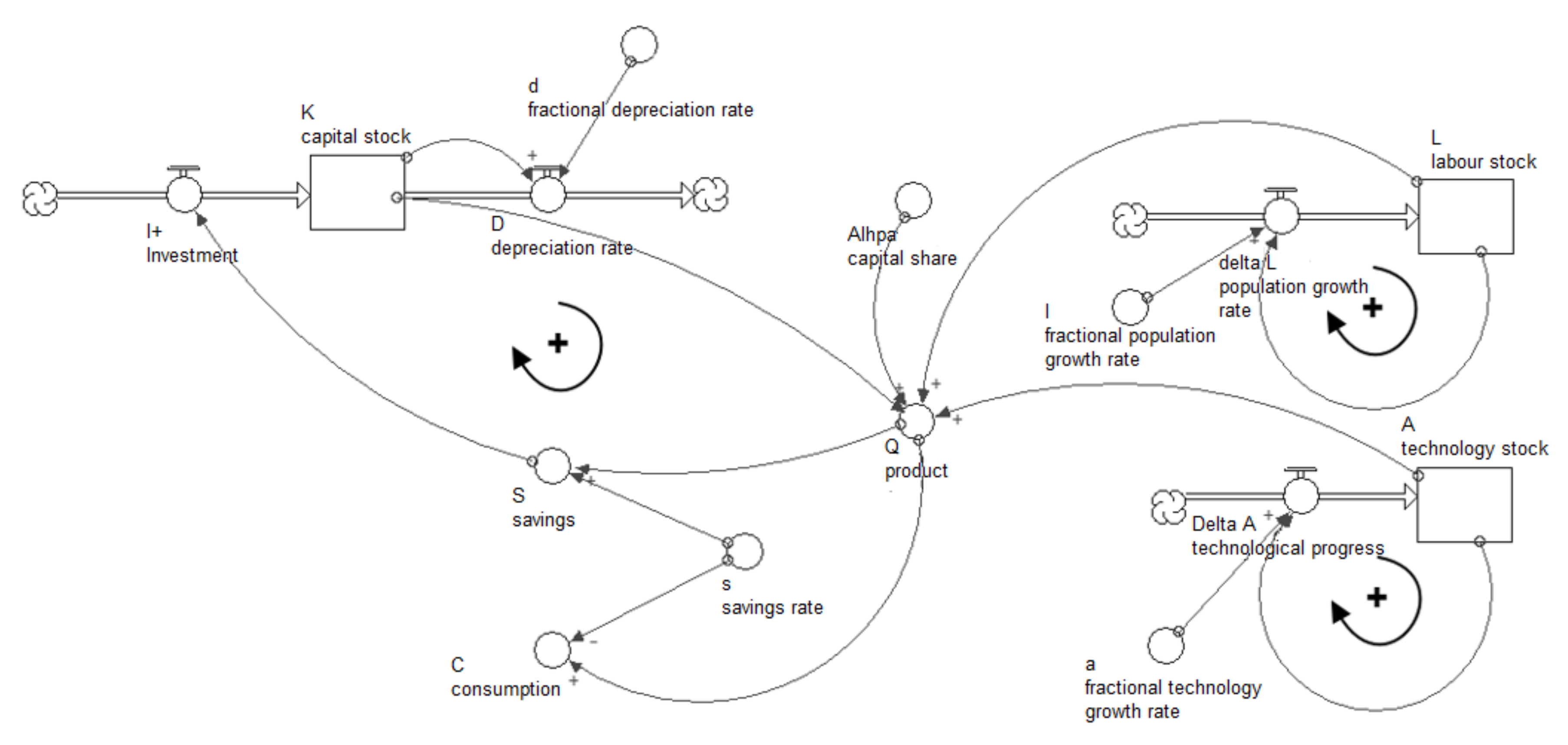
The Solow–Swan growth model consists of three stocks—the capital stock Kt, the population stock Lt (model assumes that all people work, therefore, it also represents total labour supply) and the third stock, At, which represents the state of technology.
Economic product Q is represented by the Cobb–Douglas production function:
Q t = A t K t α L t α 1 ,
where α is the capital elasticity in production. The model employs the pattern of exponential growth in two components—the labour force and technology:
L t = L 0 e l t
A t = A 0 e a t ,
where L 0 and A 0   are the stocks initial levels and l and a are their respective growth rates, and t represents the time step in the model. Capital stock is influenced by the savings, S, and depreciation rate, D. Constant share of product is saved
S t = s · Y t
and the model assumes a closed economy, therefore
I t = S t .
Depreciation rate D is defined as a constant rate of capital degradation:
D t = d · K t .
The last equation describes capital dynamics:
K t = K t 1 + ( I t D t ) .
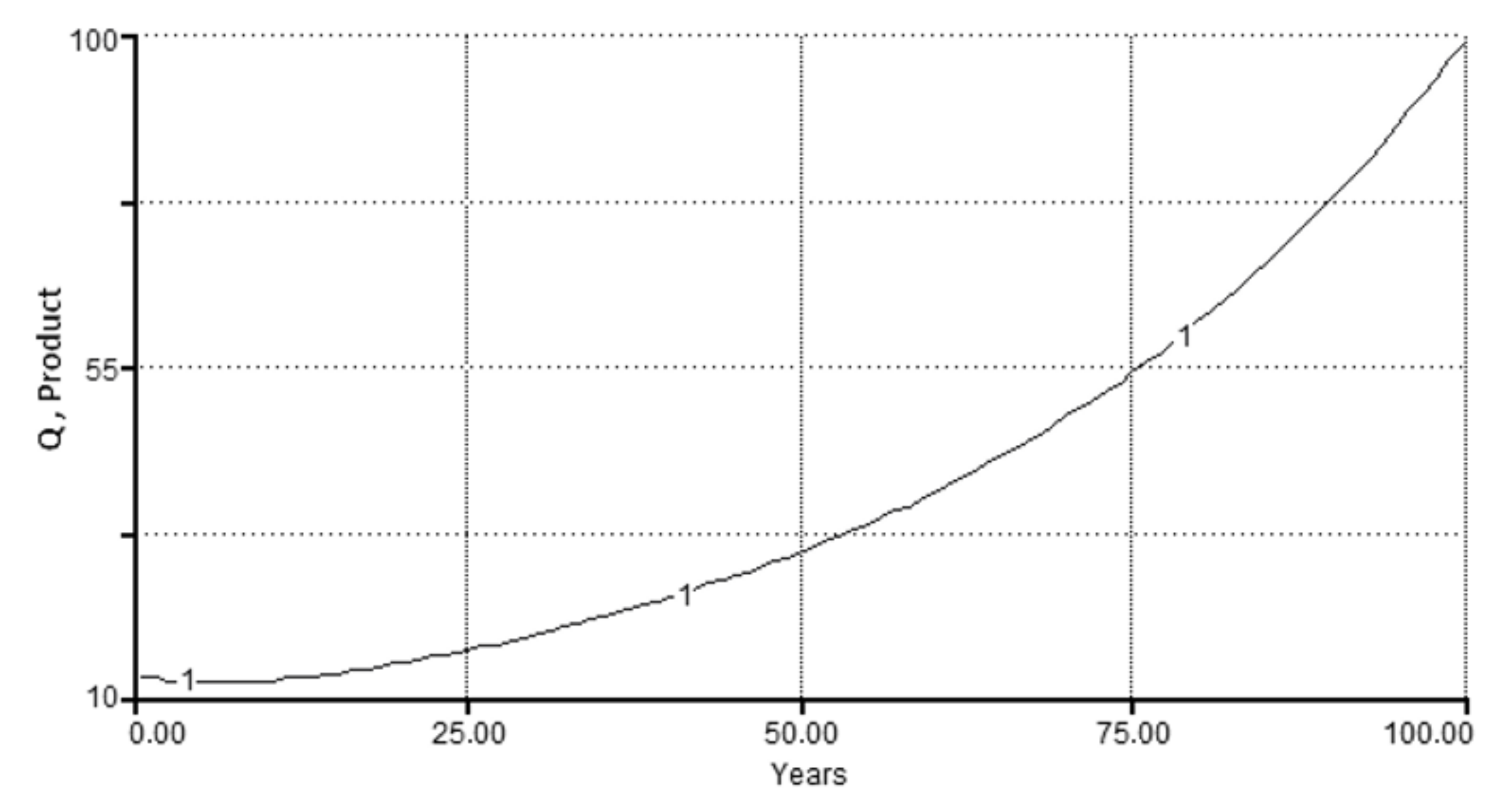
The model scheme in system dynamics notation is presented in Figure 1 alongside the representative model output in Figure 2.
Apparently, there are only local feedbacks in the model, i.e., feedbacks that do not cause a change in more than one stock, which cannot support the non-linear behaviour of the system. That alongside the presence of only positive feedback in the model, is why the final product grows without limits in Figure 2. On a similar note, another flaw is the representation of the population as a simple accumulation process, leaving out the possibility of its decline or collapse. The model thus absolutely misses the systemic perspective and the feedback structure that would capture the reality in a more realistic way.
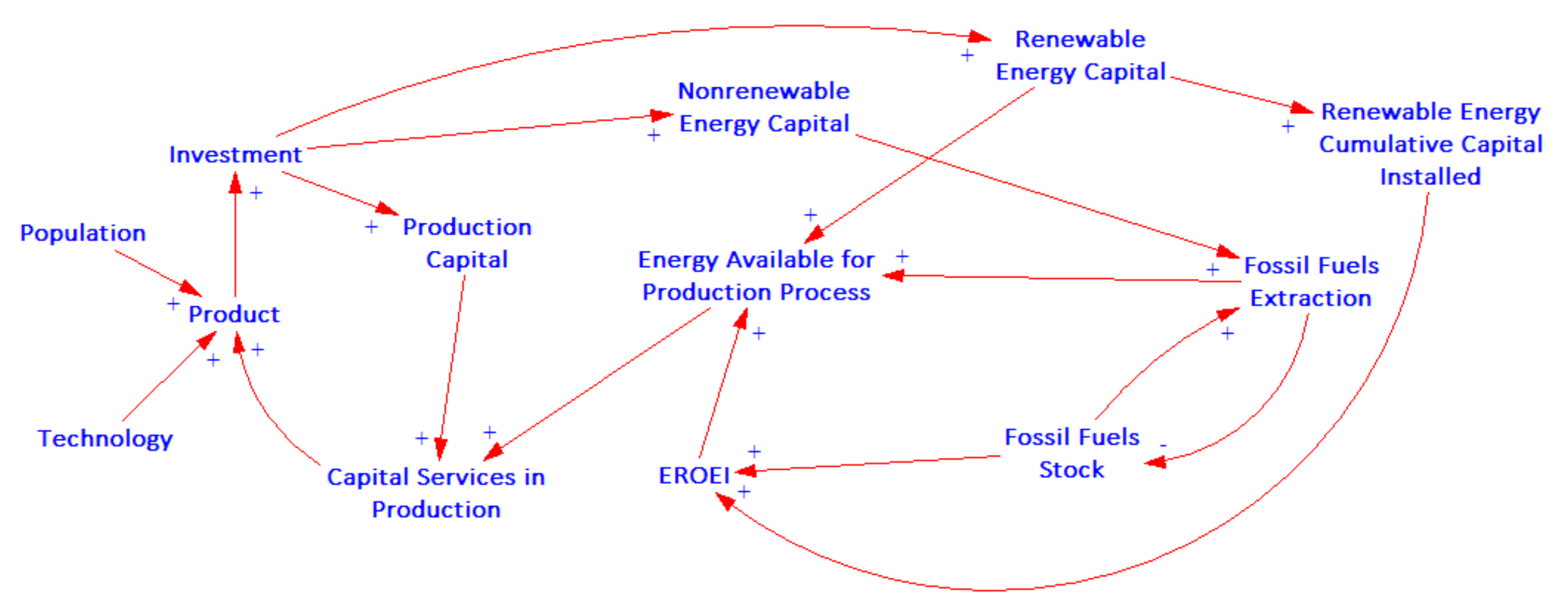
Below (Figure 3) is a causal diagram representing the extension of the model by the energy sector.
In order to be useful in the economic production, the Production Capital has to be supplied with Energy available for the production process yielding capital usable in the production process or Capital services in production. From this viewpoint, it is possible to have huge capital stock in the model, which can be increasingly useless in production in a situation of increasing energy scarcity. The equation below represents a modified Cobb–Douglas production function used by the extended version of the model, where E e t is the energy extracted and E r t is the energy required to operate the whole available capital stock:
Q t = A t ( K t E e t E r t ) α L t α 1 .
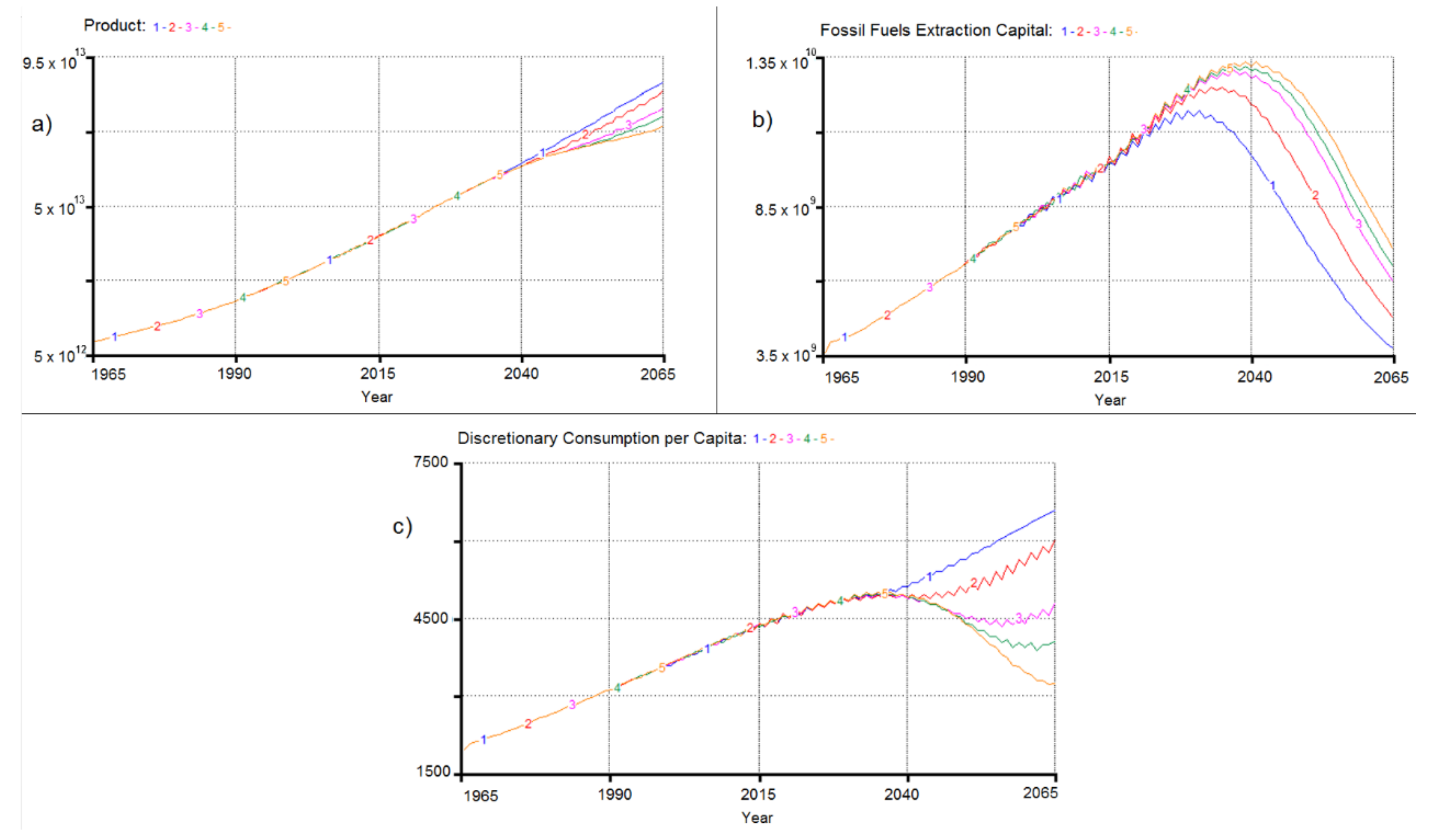
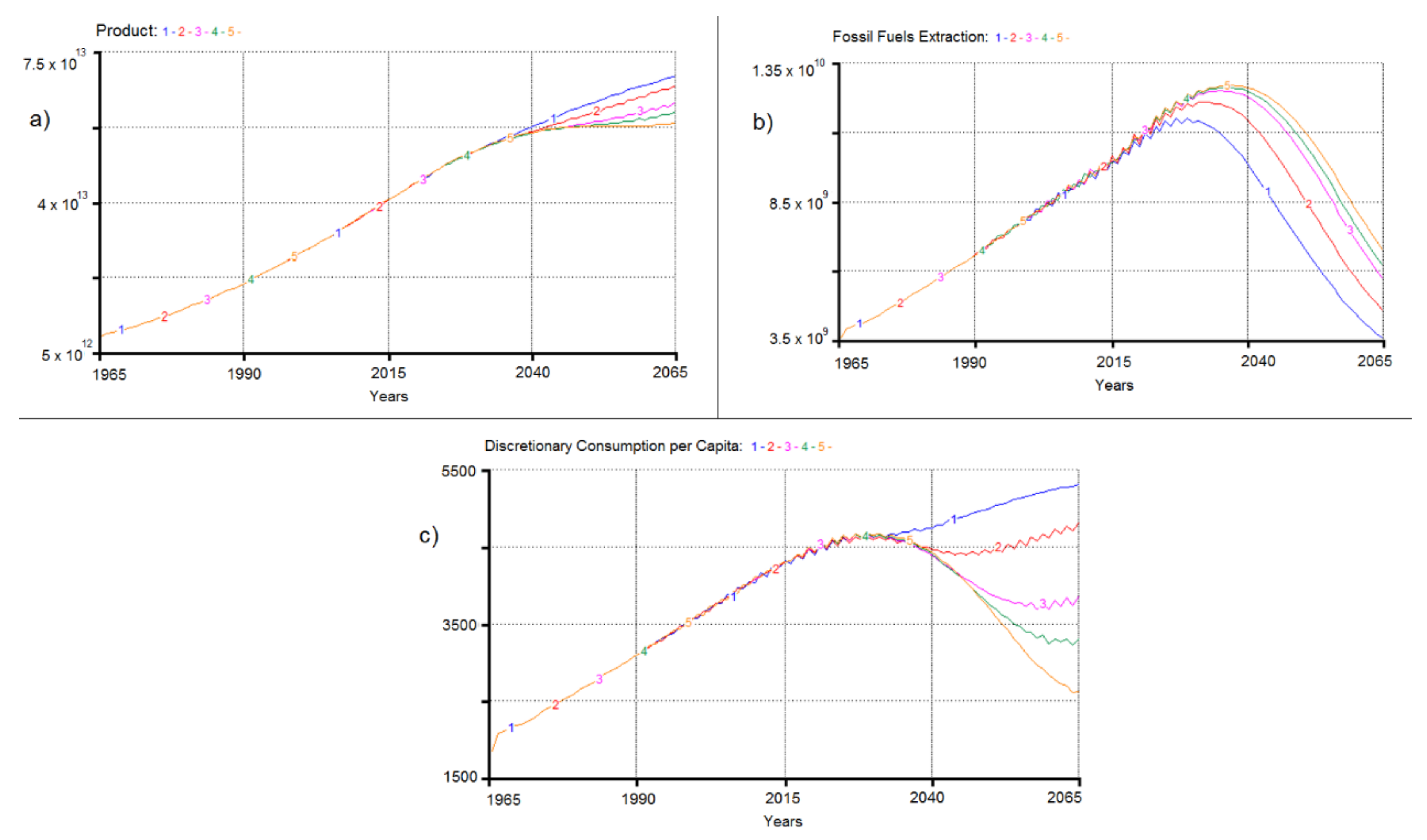
There are two other types of capital present in the model, Non-renewable energy Capital and Renewable Energy Capital. Non-renewable energy capital dominates in the model initial configuration (start year is 1950) and its increasing amount leads to a higher Fossil Fuels Extraction, which in turn supplies more Energy available for the production process. Unfortunately, Fossil Fuels Extraction leads to a reduced Fossil Fuels Stock, which in turn creates downward pressure on the Fossil Fuels Extraction and EROEI, and also imposes the total limit of energy that can be ultimately extracted. This effect introduces a negative feedback loop that can have a decisive impact on the model behaviour and output (Product). The resulting behaviour of the model can be seen as a fight for dominance between the aforementioned negative feedback loop and renewable energy loop, which in general has a reinforcing character, but Renewable Energy Capital (representing the ‘new’ renewables, Solar PV, Wind power) starts with very low EROEI values, which increase with its installed cumulative capacity. In this way, renewable resources quality determines the system performance in later periods when non-renewable energy sources are scarce.
One of the simplifying assumptions of the Solow–Swan model is that the savings rate is constant. The Ramsey–Cass–Koopmans model allows households to make optimal consumption/saving decisions as a reaction to their environment. The capital stock then reflects interactions between households supplying savings to the firms, which demands it—the savings rate is no longer constant. Households face the problem of maximizing utility subject to specific budget constraints. For this problem, economics employs the method of dynamic optimization. For simplicity, we adopt a heuristic approach instead, in which the savings rate is adjusted according to the return rate on capital, dependent on the marginal productivity of capital in production. This approach was first used by Fiddaman [41]. The model can also be simulated with a constant savings rate.
The study rationale is based on the answer to the following question: Why should such a model not be developed and tested using standard economic tools, namely various general or partial equilibrium models? Professor Keen puts it succinctly [49]:“…from neither general equilibrium nor microfoundations, but from the very sound rejection of both these concepts decades ago, by almost all the intellectual disciplines that build mathematical models apart from economics. In the mid-20th century, other modelling disciplines developed the concept of “complex systems”, along with the mathematical and computing techniques needed to handle them. These developments led them to the realisation that these systems were normally never in equilibrium—but they were nonetheless general models of their relevant fields. …Economics needs to embrace the reality that, even more so than the weather, the economy is a complex system, and it is never in equilibrium”.
The applied model is implemented in the software Stella, version 9.1.3 (ISEE Systems Inc., Lebanon, NH, USA). The representation of the model regarding system dynamics is associated with a few basic components, or sectors, as presented in Figure 4. Population sector, general purpose capital goods sector and the technology sector are typical and not very different from mainstream economic models. The production process sector is highly modified and includes effects of energy availability on capital usability in production and endogenous savings rate, which reflects the total capital amount employed in production and the availability of energy resources for its operation. The energy sector is composed of a renewable energy source and a non-renewable energy source. At the start of the simulation, the non-renewable energy source is cheap and plentiful; however, with the decline of its limited reserves, its price grows. The renewable energy source starts with a high price, which declines with its cumulative installed capacity. The energy capital investment redistribution mechanism (which divides investment between the two aforementioned energy sources) is also part of the energy sector.
The model consists of standard components (Population, Capital, Capital Energy Consumption, Technology, Output, and Investment) and additional components (Fossil Fuels sector, Renewable energies sector, Renewable energy sources learning curve, EROEI, and Energy Demand and Supply).
Below is a simplified stock-flow diagram of the model extension (see Figure 5), with pricing mechanism and EROEI computation parts excluded for clarity.
Table 1 sums up the primary variables of the model. Apparently, the model is in concordance with one of the most significant principles of systems thinking, i.e., it is as endogenous as possible. Moreover, selected essential but omitted variables are introduced. It is important to understand the limitations of the model that result from these omissions.
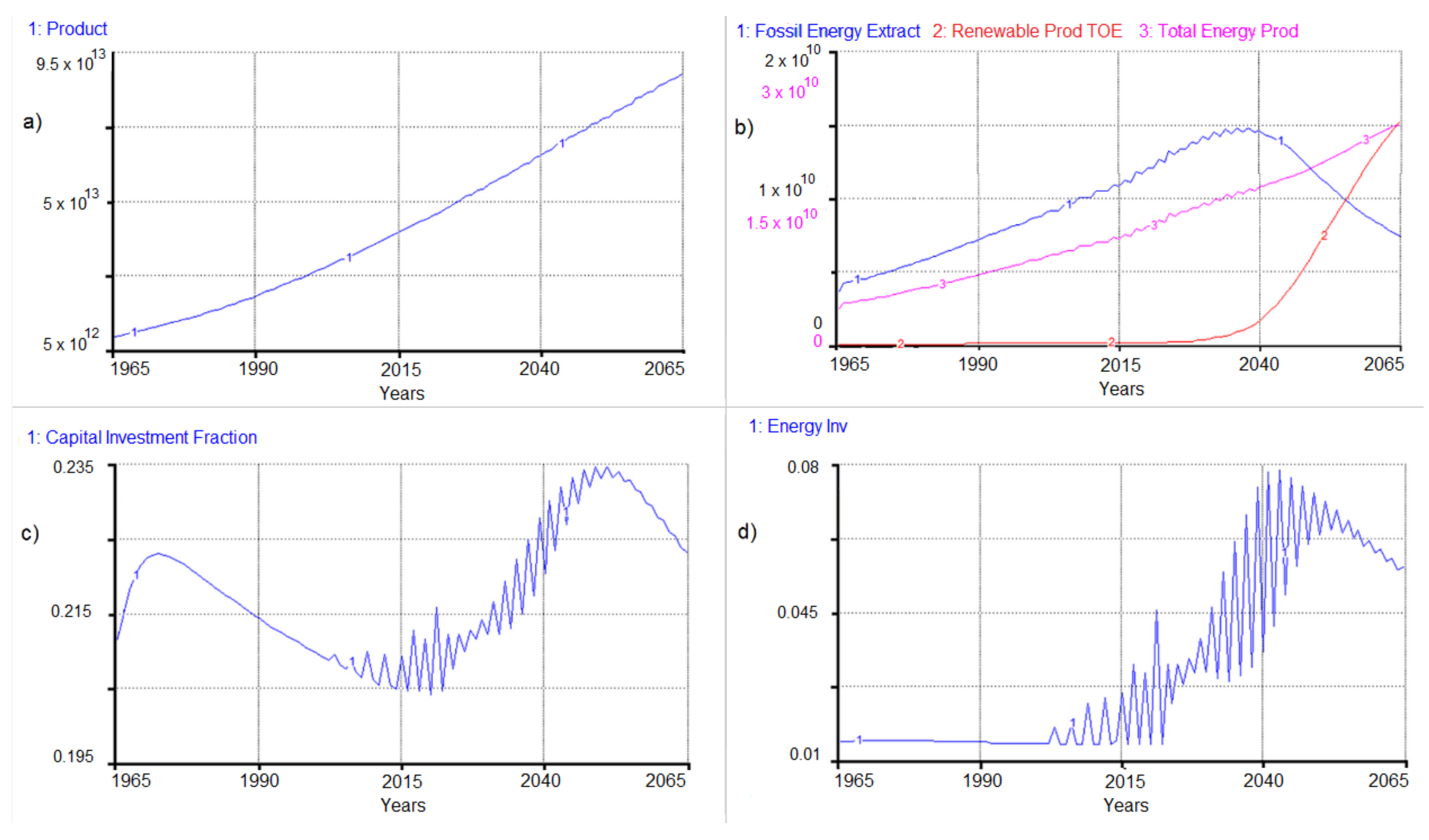
The simulation period for the model is 1965–2065. The model recreates historical behaviour over the last 50 years and then forecasts the next 50.

4. Results

The model described in the previous section is used to test two scenarios in order to find the behavioural pattern of the whole economic system. At the beginning of simulations, the initial values of variables are set. Model equations and parametrisation of variables can be found in Appendix A. Both scenarios are the same in nature and inner structure. The only difference is that there is one more assumption activated—the assumption of the end of growth of the Technology factor. This assumption is based on the work of Ayress and Warr, who associated it with the growing efficiency of transformation of energy inputs into useful work. This also means that increasing efficiency is limited by the laws of thermodynamics, which pose ultimate limits to efficiency that we are currently approaching in many energy conversion processes [50].

4.1. Model Behaviour

In Scenario 1, the capital investment rate is endogenous, dependent on the total amount of capital in production and the energy availability for capital utilization in the production process. There is almost no dip in the total energy production thanks to the variable investment rate, which helps to allocate investment into the energy sector as needed. Total energy production is also slightly higher, which helps to reach a higher GDP in this scenario. This scenario presents the endogenously adjusted investment rate, which reacts to the energy available for capital and the total amount of capital used in production.
Total capital investment varies between 22% of the total product around the year 1975, declines to around 20% in the year 2016, and then climbs almost to 24% in reaction to energy crisis created by the exhaustion of fossil fuels. Investment in the energy sector peaks in the year 2039 with the value of 8% of total product allocated for the energy sector, which is enough to keep more than 95% of capital usable in the production process most of the time.
Simulation results associated with economic growth, energy sector, total investments, and energy sector investments in Scenario 1 are presented in Figure 6.
As already mentioned, Scenario 2 is associated with activation of the assumption of the end of growth of the Technology factor. With the activation of this assumption, the growth of the technological factor almost completely stops after the year 2040, and can no longer be a primary driver of economic growth (see part a) in Figure 7). The product, in this case, reaches the value of 6.878 × 10¹³ 1989 $ only. Per capita GDP growth stops and stagnates around the level reached in the year 2030. This corresponds to the total cumulative discretionary consumption of 2.98 ×10¹⁵ 1989 $, significantly lower than in the previous scenario. Since the Technology factor fails to contribute meaningfully to economic growth after the year 2040, it leads to lower GDP and lower investment and, thanks to that smaller stock of capital goods, needs a lower amount of energy than previous scenarios. In the first scenario, capital stock reaches a level of 2.4 ×10¹⁴ 1989 $, but in this scenario it is only 1.33 × 10¹⁴ 1989 $. Thanks to this, peak extraction of fossil fuels is postponed by a few years. Total capital investment is not much different compared to the third scenario until the year 2020, when the total capital investment starts to be about 1% or 2% lower. The amount of total investment going straight into the energy sector is not much higher than in the previous scenario, and reaches a value of 10% of total product in 2040. Behaviour over time associated with economic growth, energy sector, and total investments can be seen in Figure 7.

4.2. Sensitivity Analysis

As the original model is significantly extended, there is no control measurement that could be used for evaluation of change of model behaviour. Therefore, the sensitivity analysis is performed in both Scenarios 1 and 2, while the first run of the analysis can be considered s the baseline. Varied are the following parameters: Renewable Energy Capital Lifetime, Load Factor, Price Reduction per Total Capacity Doubling, and Renewables Price. All these variables have one thing in common—they all influence the EROEI of renewable energy source. This sensitivity analysis thus explores the influence of the varied EROEI on the model. While details are presented in Table 2, acquired results can be found in Figure 8 and Figure 9 for Scenario 1, and Figure 10 and Figure 11 for Scenario 2.

4.2.1. Scenario 1

Economic growth is influenced by varied renewable energy resource parameters, but maybe less than expected. With the best renewable energy source (1), the product reaches a value of 8.689 × 10¹³ 1989 $, with the worst in run number 5 it is 7.355 × 10¹³ 1989 $.
The influence on discretionary consumption is, on the other hand, decisive. This is caused by the drastically higher investment demands in different runs. In run number 1, discretionary consumption per capita grows and reaches a total cumulative value of 3.11 × 10¹⁵ 1989 $, but in the fifth run it is only 2.82 × 10¹⁵ 1989 $, or a discretionary consumption roughly corresponding to the year 1995 (slightly above 3000 1989 $ per capita).
The influence of varied EROEI on the timing of the peak of fossil energy extraction is straightforward—the worse the renewable energy resources, the higher amounts of fossil fuels are extracted, and for longer.
Investment varies wildly with renewable resource quality: in the first run it is only a bit higher than in the preceding period with an abundance of cheap fossil fuels, at around 26% of the product; in the last scenario, a whopping 54% of product needs to be reinvested.
It is clear that the quality of the renewable energy source is a strong predictor of future wellbeing. In run 5, its EROEI is just around two, which corresponds to around 50% investment straight into the energy sector—clearly an unrealistic value. Even run 3 does not look rosy with the investment rate oscillating around 40% of total product and at around 25% of total product invested straight into the energy sector.

4.2.2. Scenario 2

As in the sensitivity analysis performed in Scenario 1, economic growth is influenced by the renewable resource quality at a similar magnitude, but the total GDP is lower thanks to the assumption activated in this scenario. The best renewable energy source (1) product reaches a value of 6.91 × 10¹³ 1989 $; at the worst in run number 5 it is 5.82 × 10¹³ 1989 $.
Discretionary consumption flattens at the same time as in the sensitivity analysis of Scenario 1 and the influence on discretionary consumption is also decisive. In run number 1, discretionary consumption per capita grows and reaches a total cumulative value of 3 × 10¹⁵ 1989 $, but in the fifth run it is only 2.62 × 10¹⁵ 1989 $ (both figures are significantly lower than the total discretionary consumption reached in the sensitivity analysis of Scenario 1), or a discretionary consumption roughly corresponding to 1975 (slightly above the value of 2500 1989 $ per capita).
Compared to the sensitivity analysis from Scenario 1, the situation here is similar, the only difference being the smaller peak values of fossil fuels extraction, which is explained by the fact that GDP growth in Scenario 2 is not as vigorous as in the first thanks to the saturation of the growth of the technological factor.
Necessary investment values are slightly below the values observed in the sensitivity analysis for Scenario 1. For example, in run 3, necessary investment rate in the year 2040 is 0.29 in Scenario 1 and 0.27 in this scenario. The difference is more pronounced in run 5, with the lowest quality of renewable power source (at around 5% in the final year of simulation).
Compared to the sensitivity analysis performed in Scenario 1, necessary investment for the energy sector is significantly lower on average for almost all runs except the first one with the renewable energy resource of the highest quality. For example, in 2040 the energy sector requires an investment of 18% of total product in Scenario 1 and 14% in this scenario.

5. Discussion

The presented model is relatively simple in structure and is not intended to serve as a basis for detailed predictions; its broad nature allows us only to sketch some probable trajectories of general trends. Despite its simplicity, it is possible to compare its results to some of the more elaborate models.
Interesting is the comparison with the Randers study 2052: A global forecast for the next 40 years. It is important to note that the model used in his study is mixed in its approach, as it partly uses system dynamics and the rest of the variables are based on a simple trend extrapolation. The Randers model also predicts continued GDP growth until 2050. The problem is that consumption share drops in extreme cases to only 60%, as the system has to cope with climate change damage and energy transitions at the same time [51]. This roughly corresponds to run 3 in the sensitivity analysis of our extended neo-classical growth model, which assumes the EROEI of new renewables will reach a value of around 5 (but our model does not take into the account damage arising from climate change).
The world limits model developed by Capellán-Pérez et al. presents another desirable comparison. However, it is important to note that this model does not use any form of production function; GDP growth is only assumed (extrapolation), so there is no feedback between the emerging energy shortages and the economic output. This constitutes an omission of a critical feedback mechanism that is left out in this model and is present in our study. The authors use the disaggregated form of resources representation, so coal, oil and gas extractions are simulated separately. The first signs of energy scarcity (meaning that the demand for energy is bigger than the supply) arise in the model at around 2020 (in the transportation sector), depending on the scenario [43]. This corresponds remarkably well to our results obtained with a much simpler, yet more feedback-rich model as the ratio of the capital used in production process vs total capital stock declines below 1 at around the same time, depending on the renewable energy source parameters.
The model feedback structure could be enriched further. A previously identified opportunity is the lack of outflow from the population stock. Both death rate and birth rate are influenced by the energy availability [14].
Acquired results reveal that achievement of successful energy transition and prevention of undesired global environmental change requires large-scale modifications of approaches in the global energy system modelling. This effort also has to be supported by system dynamists who can elaborate classical or develop new models that would incorporate selected related topics. Modelling of the energy sector is quite common in both science and engineering. Extension to economics thus represents an innovative contribution. The modelling process is a complex task regardless of the discipline. Therefore, the authors need to be sure that their models are used to (1) ensure that what is known is considered in the analysis; (2) offer a sound and consistent underlying methodological approach for decision-making; and (3) guarantee the internal consistency of the scenarios [27]. However, the main challenge associated with models is the ability to properly explore the large uncertainties inseparable from the modelling procedure [52]. Not only are uncertainties related to how the system may develop, but also how the system is expected to adapt when single parameters are modified in practice. The presented scenarios rely quite heavily on input data from socioeconomic, technical and environmental subsystems. This represents characteristics that many energy–economy models share [53].

6. Conclusions

There are many models of the environment–economy in the current scientific literature. Models focused on renewable resources deal with specific energy resources such as wind, solar energy, or tide currents, and are mostly associated with the situation in a particular country. This paper demonstrates how system dynamics can be applied during the study of existing economics models. Due to underlying methodological principles of system dynamics, the developed model goes one step further in the level of abstraction as it is oriented on the global level and considers renewable resources as one source of energy. Hence, although the model calibration is based on real data, it does not provide a prediction of specific source depletion or development in a particular region. The model itself is a representative of economic growth models based on the concrete theoretical model that has been established in the economic literature for decades. This model is extended by the energy sector in this study, which gives it a new dimension of complexity and reality. Added negative feedback represented by the environment, especially by the finiteness of fossil fuels and low quality of renewable energy source (lower EROEI), can alter model dynamics significantly, in relation to the renewable energy source capital parameters. Despite the apparent simplicity, it is able to mimic the behaviour of more elaborated models. The substantial added value of this paper, when compared to previous studies, is that in order to extend our understanding of modelling economic systems it shows how a specific modelling approach can be successfully applied in economics as a purely theoretical discipline. As single scenarios are tested, one can imply that this represents decision-making support used for the prediction of the future state of affairs. Although this application of the developed model is indeed possible, the model and presented scenarios are intended to serve as enablers of theoretical explanation of relationships among specific economic constructs based on existing mainstream model only. All the aspects mentioned above demonstrate that system dynamics can be added to the list of valuable modelling tools in this field.

Acknowledgments

The support of the Specific Research Projects “Socio-Economic Models and Autonomous Systems” and “Investments under the Industry 4.0 Concept” of FIM UHK is gratefully acknowledged. Special thanks go to Martin Král and Tomáš Nacházel for their helpfulness and assistance.

Author Contributions

L.R. conceived and designed the experiments; L.R. performed the experiments; V.B. and L.R. analysed the data; V.B. and L.R. wrote the paper.

Conflicts of Interest

The authors declare no conflict of interest.

Appendix A. Model Parametrization

Table A1. Population Parameters.
ParameterValueUnitsNotes
Initial Population3.326 × 109peopleNordhaus, DICE 1992–1994 model [54]
Initial Fractional Birth Rate0.0222 Calibrated to World Bank data [55]
Fractional Birth Rate Decline Historical0.0143 Calibrated to World Bank data [55]
Fractional Birth Rate Decline Rate Projected0.02139 Calibrated to United Nations projections [56]
Table A2. Capital Parameters.
ParameterValueUnitsNotes
Initial Capital16.03 × 10121989 US DollarsNordhaus, DICE 1992–1994 model [54]
Depreciation0.1 Nordhaus, DICE 1992–1994 model [54]
InvestmentEndogenously determined Nordhaus, DICE 1992–1994 model [54]
Table A3. Capital Energy Consumption Parameters.
ParameterValueUnitsNotes
Capital Energy Requirement Constant2.33 × 10−4TOE/1989 Constant $Result of model calibration
Capital Energy Requirement(Capital*Capital_energy_Requirement_Constant)*Energy_Saving_Technological_ProgressTOE
Energy Saving Technological ProgressIF Energy_Saving_Technology_Switch = 1 THEN INIT(Technology.Technology)/Technology.Technology ELSE (IF TIME ≤ 2015 THEN INIT(Technology.Technology)/Technology.Technology ELSE INIT(Technology.Technology)/HISTORY(Technology.Technology, 2015))dmnl
Energy Saving Technology Switch0/1dmnlUser control
Capital Future Energy RequirementCapital_Energy_Requirement*1.03TOEMatches historically observed rate of economic growth
Energy Capacity OrdersIF Product.Energy_Feedback_Switch = 1 THEN MAX (0,(Capital_Future_Energy_Requirement + Energy_Sector.Total_Energy_Sources_Capacity_Depreciation) − Energy_Sector.Total_Energy_Production) ELSE 0TOE
Table A4. Technology Parameters.
ParameterValueUnitsNotes
Initial technology level1dmnl
Fractional Technology growth Rate0.015 Nordhaus, DICE 1992–1994 model [54]
Fractional Technology growth Rate DeclineIF Usefull_Work_Hypothesis_Switch = 0 THEN 0.011 ELSE IF TIME > 2015 THEN 0.011*Fractional_Technology_Growth_Rate_Decline_Multiplier ELSE 0.011 Nordhaus, DICE 1992–1994 model [54]
Fractional_Technology_Growth_Rate_Decline_Multiplier5dmnlResults in lower total technology level, 2.1 compared to 2.5 with Usefull Work Hypothesis Switch = 0
Usefull Work Hypothesis Switch0/1 Corresponds to hypothesis of Ayres and Warr about slower growth of technology level
Table A5. Output Parameters.
ParameterValueUnitsNotes
Initial product8.519 × 10121989 US DollarsNordhaus, DICE 1992–1994 model [54]
Gama (Capital share in output)0.3 Nordhaus, DICE 1999 onward [54]
Energy Feedback Switch0/1
Operational CapitalIF Energy_Feedback_Switch = 1 THEN Capital.Capital*(MIN(1,Energy_Sector.Total_Energy_Production/Capital.Capital_Energy_Requirement)) ELSE Capital.Capital
Table A6. Investment.
ParameterValueUnitsNotes
Energy Inv NeededEnergy_Sector.Total_Necessary_Energy_Investment/Productdmnl
Exogenous Savings Rate Switch0/1 Switches investment to a constant value
Operational CapitalIF Energy_Feedback_Switch = 1 THEN Capital.Capital*(MIN(1,Energy_Sector.Total_Energy_Production/Capital.Capital_Energy_Requirement)) ELSE Capital.Capital
Initial Capital Investment Fraction0.22dmnlNordhaus, DICE 1992–1994 model [54]
Normal Return On Capital0.06dmnl
Capital Investment FractionIF Exogenous_Savings_Rate_Switch = 0 THEN MIN(1,Initial_Capital_Investment_Fraction*Indicators.Marginal_Return_on_Capital/Normal_Return_On_Capital) ELSE Initial_Capital_Investment_Fractiondmnl
Energy InvCapital_Investment_Fraction*(Energy_Capital_Investment_Fraction/100)dmnl
Energy Inv FinalMIN(Energy_Inv,Energy_Inv_Needed)dmnl
Production Capital InvestmentCapital_Investment_Fraction-Energy_Inv_Finaldmnl
Capital InvestmentProduction_Capital_Investment*Product1989 US Dollars
Energy Sector Available InvestmentEnergy_Inv_Final*Product1989 US Dollars
Table A7. Fossil Fuels Sector Parameters.
ParameterValueUnitsNotes
Energy Resources8.519 × 109TOE (Tonnes of Oil equivalent)Shafiee, Topal “An overview of fossil fuel reserve depletion time” [57]
Capital Effectiveness in Extraction1.89155 × 10−16TOE/$ 1989 US DollarCalibrated such that in 1965, primary energy extraction is 3.7302 Billion tonnes of Oil Equivalent (GTOE).
Added TOE capacity initial price403.06404311989 US DollarResult of calibration
Added TOE capacity priceIF (Fossil_Fuels_Reserves > 0) THEN MIN(6*Added_TOE_capacity_initial_price, (Added_TOE_capacity_initial_price*((Fossil_Fuels_Reserves/INIT(Fossil_Fuels_Reserves))^(−0.78)))) ELSE 0
Alternatively
IF (Fossil_Fuels_Reserves > 0) THEN (Added_TOE_capacity_initial_price*(1/((Fossil_Fuels_Reserves/INIT(Fossil_Fuels_Reserves))5))) ELSE 0
1989 US dollar
Fossil Fuels Extractive Capacity AdditionsFossils Ordered CapacityTOE
Fossil Fuels Extractive Capital Depreciation1/Fossil_Fuels_Extracting_Capital_Lifetime*Fossil_Fuels_Extraction_CapitalTOE
Fossil Fuels Extracting Capital Lifetime20Years
Fossil Fuels Energy ExtractionFossil_Fuels_Extraction_CapitalTOE/Year
Table A8. Renewable Energies Sector.
ParameterValueUnitsNotes
Renewable Energy Installed Capacity [Stock]0 [Initial]Watt
Watts to TOE conversion factor11,630,000dmnl
Hours per Year8760hours
Renewables Added TOE Capacity PriceRenewables_Price*((Watts_to_TOE_Conversion_Factor/(Load_Factor*Hours_per_Year)))1989 US Dollar/TOE
Renewables Ordered Capacity Watts(Renewables_Ordered_Capacity_TOE*Watts_to_TOE_Conversion_Factor)/(Load_Factor*Hours_per_Year)Watt
Load Factor0.20Percent of time for which is given renewable energy source operated on its maximum capacity.
Renewable Energy Capital Lifetime20Years
Renewable Energy Capital Depreciation(1/Renewable_Energy_Capital_Lifetime)*Renewable_Energy_Installed_CapacityWatts
Renewable Energy Capital Depreciation TOE(Renewable_Energy_Capital_Depreciation*Load_Factor*Hours_per_Year)/Watts_to_TOE_Conversion_FactorTOE
Renewable Energy Production TOE(Renewable_Energy_Installed_Capacity*Load_Factor*Hours_per_Year)/Watts_to_TOE_Conversion_FactorTOE
Table A9. EROEI.
Table A9. EROEI.
ParameterValueUnitsNotes
Energy Input FossilsFossils_Available_Investment*Indicators.Energy_Intensity_of_ProductTOE
Energy Output FossilsFossil_Fuels_Extracting_Capital_Lifetime*Fossils_Ordered_CapacityTOE
EROEI FossilsIF Energy_Input_Fossils > 0 THEN Energy_Output_Fossils/Energy_Input_Fossils ELSE 0dmnl
Energy Input RenewablesIndicators.Energy_Intensity_of_Product*Renewables_Available_InvestmentTOE
Energy Output RenewablesRenewables_Ordered_Capacity_TOE*Renewable_Energy_Capital_Lifetime*Capacity_Utilization_FactorTOE
EROEI RenewablesIF TIME ≥ Renewable_Energy_Investment_Start_Year AND Energy_Input_Renewables > 0 THEN Energy_Output_Renewables/Energy_Input_Renewables ELSE 0dmnl
Table A10. Energy Supply and Demand.
ParameterValueUnitsNotes
Fossils Price ShareAdded_TOE_capacity_price/Sum_of_Pricesdmnl
Renewables Price ShareRenewables_Added_TOE_Capacity_Price/Sum_of_Pricesdmnl
Sum of PricesAdded_TOE_capacity_price + Renewables_Added_TOE_Capacity_PriceConstant 1989 dollar
Fossils Investment Atractivness1/Fossils_Price_Sharedmnl
Renewables Investment AtractivnessIF TIME < Renewable_Energy_Investment_Start_Year THEN 0 ELSE 1/Renewables_Price_Sharedmnl
Atractivness SumRenewables_Investment_Atractivness+Fossils_Investment_Attractivnessdmnl
Renewables Investment ShareRenewable_Investment_Attractivness/Attractivness_Sumdmnl
Fossil Fuels Investment ShareFossils_Investment_Attractivness/Attractivness_Sumdmnl
Fossils Capacity Units per Investment ShareFossil_Fuels_Investment_Share/Added_TOE_capacity_priceTOE/share
Renewables Capacity Units per Investment ShareIF Renewables_Investment_Share > 0 THEN Renewables_Investment_Share/Renewables_Added_TOE_Capacity_Price ELSE 0TOE/Share
Investment Shares MultiplicatorCapital.Energy_Capacity_Orders/(Fossils_Capacity_Units_per_Investment_Share+Renewables_Capacity_Units_per_Investment_Share)dmnl
Fossils Demanded CapacityFossils_Capacity_Units_per_Investment_Share*Investment_Shares_MultiplicatorTOE
Renewables Demanded CapacityRenewables_Capacity_Units_per_Investment_Share*Investment_Shares_MultiplicatorTOE
Total Necessary Energy Investment(Fossil_Fuels_Investment_Share + Renewables_Investment_Share)*Investment_Shares_MultiplicatorTOE
Fossils Available InvestmentProduct.Energy_Sector_Available_Investment*Fossil_Fuels_Investment_ShareConstant 1989 dollar
Renewables Available InvestmentProduct.Energy_Sector_Available_Investment*Renewables_Investment_ShareConstant 1989 dollar
Fossils Ordered CapacityFossils_Available_Investment/Added_TOE_capacity_priceTOE
Renewables Ordered CapacityRenewables_Available_Investment/Renewables_Added_TOE_Capacity_PriceTOE

References

  1. Oil Discoveries at 70-Year Low Signal Supply Shortfall Ahead. 2016. Available online: Bloomberg.com (accessed on 24 January 2017).
  2. Patzek, T.W.; Croft, G.D. A global coal production forecast with multi-Hubbert cycle analysis. Energy 2010, 35, 3109–3122. [Google Scholar] [CrossRef]
  3. Bardi, U. Extracted How the Quest for Mineral Wealth Is Plundering the Planet; Chelsea Green Publishing: White River Junction, VT, USA, 2014; ISBN 978-1-60358-541-5. [Google Scholar]
  4. Urbinati, A.; Chiaroni, D.; Chiesa, V. Towards a new taxonomy of circular economy business models. J. Clean. Prod. 2017, 168, 487–498. [Google Scholar] [CrossRef]
  5. Vermeulen, W.J.V. Self-Governance for Sustainable Global Supply Chains: Can it Deliver the Impacts Needed? Bus. Strateg. Environ. 2015, 24, 73–85. [Google Scholar] [CrossRef]
  6. Gerrard, J.; Kandlikar, M. Is European end-of-life vehicle legislation living up to expectations? Assessing the impact of the ELV Directive on ‘green’ innovation and vehicle recovery. J. Clean. Prod. 2007, 15, 17–27. [Google Scholar] [CrossRef]
  7. Su, B.; Heshmati, A.; Geng, Y.; Yu, X. A review of the circular economy in China: Moving from rhetoric to implementation. J. Clean. Prod. 2013, 42, 215–227. [Google Scholar] [CrossRef]
  8. Geng, Y.; Zhu, Q.; Doberstein, B.; Fujita, T. Implementing China’s circular economy concept at the regional level: A review of progress in Dalian, China. Waste Manag. 2009, 29, 996–1002. [Google Scholar] [CrossRef] [PubMed]
  9. Murray, A.; Skene, K.; Haynes, K. The Circular Economy: An Interdisciplinary Exploration of the Concept and Application in a Global Context. J. Bus. Ethics 2017, 140, 369–380. [Google Scholar] [CrossRef]
  10. Schneider, A. Reflexivity in Sustainability Accounting and Management: Transcending the Economic Focus of Corporate Sustainability. J. Bus. Ethics 2015, 127, 525–536. [Google Scholar] [CrossRef]
  11. Goldsworthy, K. Design for Cyclability: Pro-active approaches for maximising material recovery. Mak. Futures 2014, 3. [Google Scholar]
  12. Wiedmann, T.O.; Schandl, H.; Lenzen, M.; Moran, D.; Suh, S.; West, J.; Kanemoto, K. The material footprint of nations. Proc. Natl. Acad. Sci. USA. 2015, 112, 6271–6276. [Google Scholar] [CrossRef] [PubMed]
  13. Brown, J.H.; Burnside, W.R.; Davidson, A.D.; DeLong, J.P.; Dunn, W.C.; Hamilton, M.J.; Mercado-Silva, N.; Nekola, J.C.; Okie, J.G.; Woodruff, W.H.; et al. Energetic Limits to Economic Growth. BioScience 2011, 61, 19–26. [Google Scholar] [CrossRef]
  14. Smil, V. Energy at the Crossroads: Global Perspectives and Uncertainties; The MIT Press: Cambridge/London, UK, 2005; ISBN 978-0-262-69324-0. [Google Scholar]
  15. Režný, L.; White, J.B. Economic Growth and Hubbert Curve. In Proceedings Part III of the International Scientific Conference—Hradec Economic Days 2013; Gaudeamus: Hradec Králové, Czech Republic, 2013; Volume 3, pp. 473–484. [Google Scholar]
  16. Steve, K. Incorporating Energy into Production Functions; Steve Keen’s Debtwatch: London, UK, 2016. [Google Scholar]
  17. Povoledo, L. Modelling the sectoral allocation of labour in open economy models. Can. J. Econ. 2017, 50, 685–710. [Google Scholar] [CrossRef]
  18. Semenychev, V.K.; Kurkin, E.I.; Semenychev, E.V.; Danilova, A.A. Multimodel forecasting of non-renewable resources production. Energy 2017, 130, 448–460. [Google Scholar] [CrossRef]
  19. Tsai, S.-B.; Xue, Y.; Zhang, J.; Chen, Q.; Liu, Y.; Zhou, J.; Dong, W. Models for forecasting growth trends in renewable energy. Renew. Sustain. Energy Rev. 2017, 77, 1169–1178. [Google Scholar] [CrossRef]
  20. Frédéric, B.; Giraudet, L.-G.; Céline, G.; Philippe, Q. Global sensitivity analysis of an energy—Economy model of the residential building sector. Environ. Model. Softw. 2015, 70, 45–54. [Google Scholar]
  21. Azad, A.K.; Rasul, M.G.; Khan, M.M.K.; Omri, A.; Bhuiya, M.M.K.; Hazrat, M.A. Modelling of Renewable Energy Economy in Australia. Energy Procedia 2014, 61, 1902–1906. [Google Scholar] [CrossRef]
  22. Omri, A. CO2 emissions, energy consumption and economic growth nexus in MENA countries: Evidence from simultaneous equations models. Energy Econ. 2013, 40, 657–664. [Google Scholar] [CrossRef]
  23. Court, V.; Jouvet, P.-A.; Lantz, F. Long-term endogenous economic growth and energy transitions. Energy J. 2018, 39. [Google Scholar] [CrossRef]
  24. Bureš, V.; Tučník, P. Complex agent-based models: application of a constructivism in the economic research. Inf. Manag. 2014, 17, 152–168. [Google Scholar] [CrossRef]
  25. Tesfatsion, L. Modeling Economic Systems as Locally-Constructive Sequential Games. J. Econ. Methodol. 2017, 24, 384–409. [Google Scholar] [CrossRef]
  26. Reiss, J. Suppes’ probabilistic theory of causality and causal inference in economics. J. Econ. Methodol. 2016, 23, 289–304. [Google Scholar] [CrossRef]
  27. Price, J.; Keppo, I. Modelling to generate alternatives: A technique to explore uncertainty in energy-environment-economy models. Appl. Energy 2017, 195, 356–369. [Google Scholar] [CrossRef]
  28. Messner, S.; Schrattenholzer, L. MESSAGE-MACRO: Linking an Energy Supply Model with a Macroeconomic Module and Solving it Iteratively. Energy Int. J. 2000, 25, 267–282. [Google Scholar] [CrossRef]
  29. Bauer, N.; Baumstark, L.; Leimbach, M. The REMIND-R model: The role of renewables in the low-carbon transformation—first-best vs. second-best worlds. Clim. Chang. 2012, 114, 145–168. [Google Scholar] [CrossRef]
  30. Fujino, J.; Nair, R.; Kainuma, M.; Masui, T.; Matsuoka, Y. Multi-gas Mitigation Analysis on Stabilization Scenarios Using Aim Global Model. Energy J. 2006, SI2006. [Google Scholar] [CrossRef]
  31. Mohanty, S.; Patra, P.K.; Sahoo, S.S.; Mohanty, A. Forecasting of solar energy with application for a growing economy like India: Survey and implication. Renew. Sustain. Energy Rev. 2017, 78, 539–553. [Google Scholar] [CrossRef]
  32. Hamzaçebi, C. Primary energy sources planning based on demand forecasting: The case of Turkey. J. Energy S. Afr. 2016, 27, 2. [Google Scholar] [CrossRef]
  33. Lee, C.-Y.; Huh, S.-Y. Forecasting new and renewable energy supply through a bottom-up approach: The case of South Korea. Renew. Sustain. Energy Rev. 2017, 69, 207–217. [Google Scholar] [CrossRef]
  34. Almeida Prado, F.; Athayde, S.; Mossa, J.; Bohlman, S.; Leite, F.; Oliver-Smith, A. How much is enough? An integrated examination of energy security, economic growth and climate change related to hydropower expansion in Brazil. Renew. Sustain. Energy Rev. 2016, 53, 1132–1136. [Google Scholar] [CrossRef]
  35. Guidolin, M.; Guseo, R. The German energy transition: Modeling competition and substitution between nuclear power and Renewable Energy Technologies. Renew. Sustain. Energy Rev. 2016, 60, 1498–1504. [Google Scholar] [CrossRef]
  36. Deng, J. Grey Management: Grey Situation Decision Making in Management Sciences. J. Grey Syst. 2004, 16, 93–95. [Google Scholar]
  37. Meadows, D.H.; Meadows, D.L.; Randers, J.; William, W.B., III. The Limits to Growth: A Report for the Club of Rome’s Project on the Predicament of Mankind, 1st ed.; Universe Books: New York, NY, USA, 1974; ISBN 978-0-87663-901-6. [Google Scholar]
  38. Turner, G. Is Global Collapse Imminent? An Updated Comparison of the Limits to Growth with Historical Data; Melbourne Sustainable Society Institute: Melbourne, Australia, 2014. [Google Scholar]
  39. Bardi, U. The Limits to Growth Revisited; SpringerBriefs in Energy; Springer: New York, NY, USA, 2011; ISBN 978-1-4419-9415-8. [Google Scholar]
  40. Sterman, J.D. The Energy Transition and the Economy: A System Dynamics Approach. Ph.D. Thesis, Massachusetts Institute of Technology, Cambridge, MA, USA, 1981. [Google Scholar]
  41. Fiddaman, T.S. Feedback Complexity in Integrated Climate-Economy Models. Ph.D. Thesis, Massachusetts Institute of Technology, Sloan School of management, Cambridge, MA, USA, 1997. [Google Scholar]
  42. Warr, B.; Ayres, R. REXS: A forecasting model for assessing the impact of natural resource consumption and technological change on economic growth. Struct. Chang. Econ. Dyn. 2006, 17, 329–378. [Google Scholar] [CrossRef]
  43. Capellán-Pérez, I.; Mediavilla, M.; de Castro, C.; Carpintero, Ó.; Miguel, L.J. Fossil fuel depletion and socio-economic scenarios: An integrated approach. Energy 2014, 77, 641–666. [Google Scholar] [CrossRef]
  44. Sgouridis, S.; Csala, D.; Bardi, U. The sower’s way: quantifying the narrowing net-energy pathways to a global energy transition. Environ. Res. Lett. 2016, 11, 094009. [Google Scholar] [CrossRef]
  45. Uehara, T.; Nagase, Y.; Wakeland, W. Integrating Economics and System Dynamics Approaches for Modelling an Ecological–Economic System. Syst. Res 2016, 33, 515–531. [Google Scholar] [CrossRef]
  46. Radzicki, M.J. System Dynamics and its Contribution to Economics and Economic Modeling. In Complex Systems in Finance and Econometrics; Meyers, R., Ed.; Springer: New York, NY, USA, 2009; pp. 727–737. ISBN 978-1-4419-7700-7. [Google Scholar]
  47. Acemoglu, D. Introduction to Modern Economic Growth; Princeton University Press: Princeton, NJ, USA, 2009; ISBN 978-0-691-13292-1. [Google Scholar]
  48. Bardi, U. Mind Sized World Models. Sustainability 2013, 5, 896–911. [Google Scholar] [CrossRef]
  49. Keen, S. Olivier Blanchard, Equilibrium, Complexity, and the Future of Macroeconomics. Available online: http://www.forbes.com/sites/stevekeen/2016/10/04/olivier-blanchard-equilibrium-complexity-and-the-future-of-macroeconomics/ (accessed on 6 November 2016).
  50. Ayres, R.; Warr, B. The Economic Growth Engine: How Energy and Work Drive Material Prosperity, Reprint ed.; Edward Elgar Publishing: Cheltenham, UK, 2010; ISBN 978-1-84980-435-6. [Google Scholar]
  51. Randers, J. 2052—A Global Forecast for the Next Forty Years Using a Mix of Models. Available online: https://www.cse.iitb.ac.in/~damani/ctaraReading/RandersFuture2052.pdf (accessed on 3 November 2016).
  52. Peterson, S. Uncertainty and economic analysis of climate change: A survey of approaches and findings. Environ. Model. Assess. 2006, 11, 1–17. [Google Scholar] [CrossRef]
  53. Bosetti, V.; Marangoni, G.; Borgonovo, E.; Diaz Anadon, L.; Barron, R.; McJeon, H.C.; Politis, S.; Friley, P. Sensitivity to energy technology costs: A multi-model comparison analysis. Energy Policy 2015, 80, 244–263. [Google Scholar] [CrossRef]
  54. Nordhaus, W.; Sztorc, P. DICE 2013R: Introduction and User’s Manual. Available online: http://www.econ.yale.edu/~nordhaus/homepage/documents/DICE_Manual_100413r1.pdf (accessed on 30 October 2016).
  55. The World Bank. Population, Total. Available online: http://data.worldbank.org/indicator/SP.POP.TOTL (accessed on 6 November 2016).
  56. United Nations World Population Prospects, Key Findings and Advance Tables. Available online: https://esa.un.org/unpd/wpp/Publications/Files/Key_Findings_WPP_2015.pdf (accessed on 6 November 2016).
  57. Shafiee, S.; Topal, E. An Overview of Fossil Fuel Reserve Depletion Time. Available online: www.iaee.org/en/publications/proceedingsabstractdoc.aspx?id=1092 (accessed on 16 January 2018).
Figure 1. Solow–Sawn growth model in system dynamics notation. Source: own work.
Systems 06 00008 g001
Figure 2. The representative output of the Solow–Swan growth model. Source: own work.
Systems 06 00008 g002
Figure 3. Simplified causal diagram of the model extension. Source: own work.
Systems 06 00008 g003
Figure 4. Overview of the basic model blocks. Source: own work.
Systems 06 00008 g004
Figure 5. Simplified stock-flow diagram of the model extension. Source: own work.
Systems 06 00008 g005
Figure 6. Scenario 1 simulation results: (a) GDP growth in Scenario 1, Y-axis—1989 $; (b) Energy sector, Y-axis—Energy production/consumption in tonnes of oil equivalent, Lines identification: 1—Fossil fuels energy extraction, 2—Renewables energy production, 3—Total energy sector energy production; (c) Total investment in Scenario 1, Y-axis—the percentage of the total product; (d) Energy sector investment, Y-axis—the percentage of the total product. Source: own work.
Systems 06 00008 g006
Figure 7. Scenario 2 simulation results: (a) Different Technology growth rates without (1) and with (2) useful work assumption activated. Y-axis—dimensionless; (b) GDP growth in Scenarios 1 and 2. Y-axis—1989 $; (c) Energy sector situation in Scenario 2, Y-axis—Energy production/consumption in Tonnes of oil equivalent, Lines identification: 1—Fossil fuels energy extraction, 2—Renewables energy production, 3—Total energy sector energy production; (d) Total investment in Scenarios 1 (blue line) and 2 (red line). Y-axis—the percentage of the total product. Source: own work.
Systems 06 00008 g007
Figure 8. Sensitivity analysis in Scenario 1: (a) GDP growth with varied EROEI in Scenario 1. Y-axis—1989 $; (b) Influence of varied EROEI rate on the timing of the peak of fossil fuels energy extraction in Scenario 1. Y-Axis—TOE; (c) Discretionary consumption development with varied renewable energy resource EROEI in Scenario 1, Y-axis—1989 $ per capita. Source: own work.
Systems 06 00008 g008
Figure 9. Sensitivity analysis in Scenario 1: (a) Influence of varied EROEI rate on Total Capital Investment in Scenario 1, Y-axis—Investment as a percentage of the total product; (b) EROEI of renewable energy source with its varied parameters in Scenario 1; (c) Influence of varied EROEI rates on Energy sector investment in Scenario 1. Y-Axis—Percentage of the total product. Source: own work.
Systems 06 00008 g009
Figure 10. Sensitivity analysis in Scenario 2: (a) GDP growth in the scenario with varied EROEI in Scenario 2. Y-axis—1989 $; (b) Influence of varied EROEI rate on the timing of the peak of fossil fuels energy extraction in Scenario 2. Y-Axis—TOE; (c) Discretionary consumption development with varied renewable energy resource EROEI in Scenario 2, Y-axis—1989 $ per capita. Source: own work.
Systems 06 00008 g010
Figure 11. Sensitivity analysis in Scenario 2: (a) Influence of varied EROEI rate on Total Capital Investment in Scenario 2, Y-axis—Investment as a percentage of the total product; (b) EROEI of renewable energy source with its varied parameters in Scenario 2; (c) Influence of varied EROEI rates on energy sector investment in Scenario 2. Y-Axis—Percentage of the total product. Source: own work.
Systems 06 00008 g011
Table 1. Model variables. Source: own work.
Endogenous VariablesExogenous VariablesOmitted Elements
Macroeconomic productPopulationAtmosphere
ConsumptionOutput elasticity with respect to capital ( α )Emissions of CO2
Savings/InvestmentTechnologyNatural resources of non-energy nature
Capital
Role of energy in creation of macroeconomic product
Extraction and depletion of fossil fuels
Renewable energy sources
Demand for energy sources
Representation of EROEI
Table 2. Parameter values in the sensitivity analysis of Scenarios 1 and 2. Source: own work.
Run NumberRenewable Energy Capital Lifetime (Years)Load Factor (Dimensionless)Price Reduction per Total Capacity Doubling (Dimensionless)Renewables Price per Watt of Installed Capacity (1989 $)
1300.30.1510
2270.250.12512
3240.20.115
4200.150.117
5180.10.120

