Article

Improved Time Response of Stabilization in Synchronization of Chaotic Oscillators Using Mathematica

1
College of Applied Sciences, Ministry of Higher Education, Nizwa 611, Sultanate of Oman
2
School of Quantitative Sciences, College of Arts & Sciences, UUM, Keddha 06010, Malaysia
*
Author to whom correspondence should be addressed.
Systems 2016, 4(2), 25; https://doi.org/10.3390/systems4020025
Submission received: 27 December 2015 / Revised: 31 March 2016 / Accepted: 15 June 2016 / Published: 22 June 2016

Abstract

:
Chaotic dynamics are an interesting topic in nonlinear science that has been intensively studied during the last three decades due to its wide availability. Motivated by much researches on synchronization, the authors of this study have improved the time response of stabilization when parametrically excited Φ6—Van der Pol Oscillator (VDPO) and Φ6—Duffing Oscillator (DO) are synchronized identically as well as non-identically (with each other) using the Linear Active Control (LAC) technique using Mathematica. Furthermore, the authors have synchronized the same pairs of the oscillators using a more robust synchronization with faster time response of stability called Robust Adaptive Sliding Mode Control (RASMC). A comparative study has been done between the previous results of Njah’s work and our results based on Mathematica via LAC. The time response of stabilization of synchronization using RASMC has been discussed.

1. Introduction

The study of chaotic behavior in nonlinear systems has attracted much attention because of many possible applications in various fields of science and technology. Most of the research has been devoted to the modeling of new chaotic systems together with the control and synchronization [1]. Thus far much work based on modeling, as well as various new control and synchronization techniques, has been carried out and is worth citing. For example, the sliding mode control [2,3,4,5], adaptive control [6,7,8], linear active control [9,10,11,12,13], linear feedback control [14,15,16], projective synchronization [17,18,19], nonlinear active control [20,21] and backstepping control [22], to mention but a few.
A recent study of Shahzad [23] focused the attention of researchers on how to choose a model based synchronization technique and the appropriate mathematical tools for simulation. Pourmahmood et al. [24] have developed a Robust Adaptive Sliding Mode Control (RASMC) and implemented it successfully on three well known chaotic systems (Lorenz, Chen and Liu) using MATLAB for all of the simulations, but when the same study was done using Mathematica by Shahzad [23], remarkable changes were observed in terms of time response to stabilize the synchronization.
Motivated by the aforementioned studies, we synchronize the identical and non-identical pairs of Φ6—VDPO and DO using the LAC and RASMC, respectively. However, the synchronization of Φ6—VDPO and DO using the LAC has already been done by Njah [12] but when the same work of Njah [12] was repeated via LAC and using Mathematica, remarkable changes had been found in the time response of stabilization of synchronization. On the other hand, the faster time response of stabilization of synchronization performances of the RASMC forced us to implement it on the same pairs of systems studied by Njah [12]. To the best of our knowledge, this kind of study has never been done before. The main objective behind the implementation of RASMC is that the sliding mode control is one of the robust control methods and has many interesting features such as low sensitivity to external disturbances and robustness to the plant uncertainties due to structural variations and un-modeled dynamics. The sliding mode controller is composed of an equivalent control part that describes the behavior of the system when the trajectories stay over the sliding surface and a variable structure control part that enforces the trajectories to reach the sliding surface and remain on it evermore. The adaptive control is a suitable approach to overcome system uncertainties, especially uncertainties derived from uncertain parameters. The adaptive sliding mode control has the advantages of combining the robustness of the sliding mode control with the tracking facilities of the adaptive control ([24], and the references therein).
The rest of the paper has been organized as follows: In Section 2, the three identical pairs of Φ6—VDPO and DO, respectively, and non-identical pairs of Φ6—VDPO and DO have been synchronized using the LAC. Section 3 is devoted to the brief description of RASMC as well as its implementation on identical synchronization of Φ6—VDPO and DO, respectively, and non-identical pair of Φ6—VDPO and DO. Lastly, the whole study has been concluded in Section 4.

2. Synchronization Using LAC

In this section, we synchronize the identical and non-identical pairs of Φ6—VDPO and DO, respectively, using the LAC technique for chaos synchronization that was proposed by Bai and Lonngren [9] and it has recently been accepted as one of the most efficient techniques for synchronizing both identical and non-identical chaotic systems because of its simple implementation in practical systems [25,26,27,28]. It can be easily designed according to the given conditions of the chaotic system as a way of accomplishing synchronization globally asymptotically, if the nonlinearity of the system is known. There are no derivatives in the controller and no need to calculate the Lyapunov exponents to execute the controller. These characteristics give an advantage to the technique over other conventional synchronization techniques.

2.1. Description of the Models

Since the chaotic systems are very complex nonlinear systems, they are exceptionally sensitive to tiny changes in their initial conditions and parameters variations. With the passage of time and due to the potential applications of chaotic systems in certain scientific fields, many chaotic and hyperchaotic systems have been investigated (Lorenz, Chen and Liu, etc.). In this direction, the Φ6—VDPO and DO are periodically self-excited and have rich applications in various disciplines like electronics, physics, engineering, neurology and biological sciences [29,30,31]. Njah [12] studied and investigated the synchronizations of Φ6—VDPO and DO with applications to secure communication using the LAC technique based on the Lyapunov stability theory and the Routh-Hurwitz criterion. The synchronization schemes have been studied without considering the external disturbances and model uncertainties. However, in practical applications, either environmental changes (noise) may occur any time or lack of parameters knowledge may disturb the stability of the synchronized system and this uncertainty or environmental noise cannot be simply ignored.
The Φ6—VDPO and DO are classical examples of self-oscillatory and periodic systems and are now considered as very valuable mathematical models that can be utilized in much more complex and modified systems. In these models, there exist two frequencies, namely periodic forcing and self-oscillations. The energy is generated at low amplitudes and dissipated at high amplitude. The dynamics of chaotic parametrically excited Φ6—VDPO [12] are given by the following mathematical model:
Φ 6 VDPO : x ¨ μ 1 ( 1 x 2 ) x ˙ + α 1 { 1 + η 1 cos ( 2 ω 1 t ) } x + β 1 x 3 + λ 1 x 5 = f 1 cos ω 1 t
The dynamics of another chaotic parametrically excited Φ6—DO [12] are given by the following mathematical model:
Φ 6 DO :   x ¨ + μ 2 x ˙ + α 2 { 1 + η 2 cos ( 2 ω 2 t ) } x + β 2 x 3 + λ 2 x 5 = f 2 cos ω 2 t
where the Φ6—VDPO and DO exhibit chaotic attractors for the following parameter values: μ 1 = 0.4 , α = 1.0 , β = 0.7 , λ 1 = 0.1 , η 1 = 0.7 , f 1 = 9 , ω 1 = 3.14 and μ 2 = 0.4 , α 2 = 0.46 , β 2 = 1 , λ 2 = 0.1 , f 2 = 4.5 , η 2 = 0.7 , ω 2 = 0.86 , respectively [12].

2.2. Synchronization of Two Identical Φ6—VDPO Oscillators via LAC

To achieve synchronization between two identical Φ6—VDPO, let us consider the master–slave systems synchronization scheme for two coupled identical chaotic Φ6—VDPO that can be written by choosing x = x 1 and x ˙ 1 = x 2 and x = y 1 and x ˙ = y 2 in Equation (1) for master and slave systems, respectively, as follows:
Master System : { x ˙ 1 = x 2 , x ˙ 2 = μ 1 ( 1 x 1 2 ) x 2 α 1 { 1 + η 1 cos ( 2 ω 1 t ) } x 1 β 1 x 1 3 λ 1 x 1 5 + f 1 cos ω 1 t
Slave System : { y ˙ 1 = y 2 + u 1 ( t ) , y ˙ 2 = μ 1 ( 1 y 1 2 ) y 2 α 1 { 1 + η 1 cos ( 2 ω 1 t ) } y 1 β 1 y 1 3 λ 1 y 1 5 + f 1 cos ω 1 t + u 2 ( t )
where [ x 1 ( t ) ,   x 2 ( t ) ] T and [ y 1 ( t ) ,   y 2 ( t ) ] T R 2 are the state variables of master and slave systems, respectively; μ 1 , α 1 , β 1 , λ 1 , f 1 , η 1 and ω 1 are the parameters involved in Equations (3) and (4) and u ( t ) = [ u 1 ( t ) , u 2 ( t ) ] T R 2 × 1 are the control inputs yet to be determined.
Now, the error dynamics ( e i = y i x i , for i = 1 , 2 ) from Equations (3) and (4) can be written as follows:
e ˙ 1 = e 2 + u 1 ( t ) e ˙ 2 = μ 1 e 1 μ 1 ( y 1 2 y 2 x 1 2 x 2 ) α 1 { 1 + η 1 cos ( 2 ω 1 t ) } e 1 β 1 ( y 1 3 x 1 3 ) λ 1 ( y 1 5 x 1 5 ) + u 2 ( t )
In order to make the error dynamics linear, let us redefine u 1  &  u 2 as follows:
u 1 ( t ) = v 1 ( t ) u 2 ( t ) = μ 1 ( y 1 2 y 2 x 1 2 x 2 ) + β 1 ( y 1 3 x 1 3 ) + λ 1 ( y 1 5 x 1 5 ) + v 2 ( t )
Now the linear error dynamical system can be written as:
e ˙ 1 = e 2 + v 1 ( t ) e ˙ 2 = μ 1 e 1 α 1 { 1 + η 1 cos ( 2 ω 1 t ) } e 1 + v 2 ( t )
The linear error dynamics (Equation (7)) is controlled by v 1 ( e 1 , e 2 ) and v 2 ( e 1 , e 2 ) that are defined as: ( v 1 v 2 ) = D ( e 1 e 2 ) where D = ( a b c d ) is a constant feedback matrix yet to be determined and the error dynamics (Equation (7)) can be written as: ( e ˙ 1 e ˙ 2 ) = C ( e 1 e 2 ) where C = ( a 1 + b c α 1 { 1 + η 1 cos ( 2 ω 1 t ) } μ 1 + d ) is the coefficient matrix. According to the Lyapunov stability theory and Routh–Hurwitz criteria, choose a + d + μ 1 < 0 and { c α 1 ( 1 + η 1 cos 2 ω 1 t ) } ( 1 + b ) a ( μ 1 + d ) < 0 for the stabilization of the synchronization of Equations (3) and (4).
Let a + d + μ 1 = { c α 1 ( 1 + η 1 cos 2 ω 1 t ) } ( 1 + b ) a ( μ 1 + d ) = E for E > 0 . We choose a = b = 0 and E = 1 , which yields u 1 ( t ) = 0 and u 2 ( t ) = μ 1 ( y 1 2 y 2 x 1 2 x 2 ) + β 1 ( y 1 3 x 1 3 ) + λ 1 ( y 1 5 x 1 5 ) + { α 1 ( 1 + η 1 cos 2 ω 1 t ) E } e 1 ( μ 1 + E ) e 2 .
For the same values of parameters ( μ 1 = 0.4 , α 1 = 1 , β 1 = 0.7 , λ 1 = 0.1 , f 1 = 9 , η 1 = 0.7 , ω 1 = 3.14 and E = 1 ) and initial conditions ( x 1 ( 0 ) = 0.1 ; x 2 ( 0 ) = 0.2 ; y 1 ( 0 ) = 2.2 ; y 2 ( 0 ) = 0.05 ) taken by [12], we have repeated all simulations using Mathematica. The following are the graphs of synchronization of two identical Φ6—VDPO oscillators:

2.3. Synchronization for Two Identical Φ6—DO via LAC

To achieve synchronization between two identical Φ6—DO, let us consider the master–slave systems synchronization scheme for two coupled identical chaotic Φ6—DO that can be written by taking x = x 1 and x ˙ 1 = x 2 and x = y 1 and x ˙ = y 2 in Equation (2) for master and slave systems, respectively, as follows:
Master System : { x ˙ 1 = x 2 , x ˙ 2 = μ 2 x 2 α 2 { 1 + η 2 cos ( 2 ω 2 t ) } x 1 β 2 x 1 3 λ 2 x 1 5 + f 2 cos ω 2 t
Slave System : { y ˙ 1 = y 2 + u 1 ( t ) , y ˙ 2 = μ 2 y 2 α 2 { 1 + η 2 cos ( 2 ω 2 t ) } y 1 β 2 y 1 3 λ 2 y 1 5 + f 2 cos ω 2 t + u 2 ( t )
where [ x 1 ( t ) ,   x 2 ( t ) ] T and [ y 1 ( t ) ,   y 2 ( t ) ] T R 2 are the state variables; μ 2 , α 2 , β 2 , λ 2 , f 2 , η 2 and ω 2 are the parameters involved in Equations (8) and (9); and u ( t ) = [ u 1 ( t ) , u 2 ( t ) ] T R 2 × 1 are the control inputs yet to be determined.
Using LAC technique as in Section 2.2, someone can find the controllers u 1 ( t ) = 0 and u 2 ( t ) = β 2 ( y 1 3 x 1 3 ) + λ 2 ( y 1 5 x 1 5 ) + { α 2 ( 1 + η 2 cos 2 ω 2 t ) E } e 1 + ( μ 2 E ) e 2 . For the same values of parameters ( μ 2 = 0.4 , α 2 = 0.46 , β 2 = 1 , λ 2 = 0.1 , f 2 = 4.5 , η 2 = 0.7 , ω 2 = 0.86 and E = 1 ) and initial conditions ( x 1 ( 0 ) = 0 ; x 2 ( 0 ) = 1.5 ; y 1 ( 0 ) = 0.5 ; y 2 ( 0 ) = 1 ) as taken by Njah [12], we have repeated all simulations using Mathematica. The following are the graphs of synchronization of two identical Φ6—DO:

2.4. Synchronization for Φ6—VDPO and DO via LAC

To achieve synchronization between Φ6—VDPO and DO, let us consider the master-slave systems synchronization scheme for two coupled Φ6—VDPO and DO that can be written by taking x = x 1 and x ˙ 1 = x 2 and x = y 1 and x ˙ = y 2 in Equations (1) and (2) for master and slave systems, respectively, as follows:
Master System : { x ˙ 1 = x 2 , x ˙ 2 = μ 1 ( 1 x 1 2 ) x 2 α 1 { 1 + η 1 cos ( 2 ω 1 t ) } x 1 β 1 x 1 3 λ 1 x 1 5 + f 1 cos ω 1 t
Slave System : { y ˙ 1 = y 2 + u 1 ( t ) , y ˙ 2 = μ 2 y 2 α 2 { 1 + η 2 cos ( 2 ω 2 t ) } y 1 β 2 y 1 3 λ 2 y 1 5 + f 2 cos ω 2 t + u 2 ( t )
where [ x 1 ( t ) ,   x 2 ( t ) ] T and [ y 1 ( t ) ,   y 2 ( t ) ] T R 2 are the state variables of master and slave systems; μ 1 , α 1 , β 1 , λ 1 , f 1 , η 1 , ω 1 , μ 2 , α 2 , β 2 , λ 2 , f 2 , η 2 and ω 2 are the parameters involved in Equations (10) and (11) and u ( t ) = [ u 1 ( t ) , u 2 ( t ) ] T R 2 × 1 are the control inputs yet to be determined.
Using LAC technique, as it has been implemented in the last two subsections, someone can find the controllers:
u 1 ( t ) = 0 u 2 ( t ) = ( μ 1 + μ 2 ) x 2 μ 1 x 1 2 x 2 + α 2 ( 1 + η 2 cos 2 ω 2 t ) x 1 α 1 ( 1 + η 1 cos 2 ω 1 t ) x 1 + β 2 y 1 3 β 1 x 1 3 + λ 2 y 1 5 λ 1 x 1 5 f 2 cos ω 2 t + f 1 cos ω 1 t + { α 2 ( 1 + η 2 cos 2 ω 2 t ) E } e 1 + ( μ 2 E ) e 2
For the same values of parameters ( μ 1 = 0.4 , α 1 = 1 , β 1 = 0.7 , λ 1 = 0.1 , f 1 = 9 , η 1 = 0.7 , ω 1 = 3.14 , μ 2 = 0.4 , α 2 = 0.46 , β 2 = 1 , λ 2 = 0.1 , f 2 = 4.5 , η 2 = 0.7 , ω 2 = 0.86 and E = 1 ) and initial conditions ( x 1 ( 0 ) = 0.1 ; x 2 ( 0 ) = 0.2 ; y 1 ( 0 ) = 0 ; y 2 ( 0 ) = 1.5 ) as taken by Njah [12], we have repeated all simulations using Mathematica. The following are the graphs of synchronization of Φ6—VDPO and DO.

2.5. Results and Discussions

In Section 2.2, Section 2.3 and Section 2.4, three different pairs of Φ6—VDPO and DO have been synchronized using LAC technique. In our study, all simulations are based on Mathematica that provide us the remarkable changes in the time of stabilization of synchronization. Earlier, in the same study of Njah [12], for identical pairs of Φ6—VDPO and non-identical pairs (i.e., Φ6—VDPO and DO), controllers were activated at around t = 60 and for identical pairs of Φ6—DO, the controllers were activated at around t = 100 . On the other hand, for the same pairs and same technique (LAC) if Mathematica is being used, someone can observe the remarkable changes in the time of stabilization (Figure 1, Figure 2, Figure 3, Figure 4, Figure 5, Figure 6, Figure 7, Figure 8, Figure 9, Figure 10, Figure 11, Figure 12 and Figure 13). In our study, for all of the cases, not only do controllers activate around t = 4 but secure communication scheme (Figure 3, Figure 4, Figure 7, Figure 8, Figure 11 and Figure 12), convergence of errors defined by e ( t ) = e 1 2 ( t ) + e 2 2 ( t ) (Figure 13) also start to stabilize at the same time when simulation is done using Mathematica. Furthermore, it may also be observed that the error states converged to the origin in the range of [−0.5, 1.5] very smoothly and quickly as compared to the work done by Njah [12]. These features give advantages to the current study.

3. Synchronization Using RASMC

In this section, we synchronize the identical and non-identical pairs of Φ6—VDPO and DO using RASMC technique that has a very quick response in stabilizing the synchronization of chaotic systems [32,33,34,35,36]. Below we describe the technique in details.

3.1. Description of RASMC

For the n-dimensional master and slave systems with external uncertainties, disturbances and unknown parameters, the RASMC [24] is described as follows:
M a s t e r   s y s t e m : x ˙ ( t ) = f ( x ) + F ( x ) θ + Δ f ( x , t ) + d m ( t )
S l a v e   S y s t e m : y ˙ ( t ) = g ( y ) + G ( y ) ψ + Δ g ( y , t ) + d s ( t ) + u ( t )
where x ( t ) = [ x 1 , x 2 , , x n ] T are the state vectors, f ( x ) = [ f 1 ( x ) , f 2 ( x ) , , f n ( x ) ] T are the continuous nonlinear functions, F i ( x ) ,   i = 1 , 2 , , n , is i t h row of an n × n matrix ( F ( x ) ) whose elements are continuous nonlinear functions, θ = [ θ 1 , θ 2 , , θ n ] T are the unknown vector parameters, and Δ f ( x , t ) = [ Δ f 1 ( x , t ) , Δ f 2 ( x , t ) , , Δ f n ( x , t ) ] T and d m ( t ) = [ d 1 m ( t ) , d 2 m ( t ) , , d n m ( t ) ] T are the vectors of unknown uncertainties and external disturbances of the master system, respectively. y ( t ) = [ y 1 , y 2 , , y n ] T are the state vectors, g ( y ) = [ g 1 ( y ) , g 2 ( y ) , , g n ( y ) ] T are the continuous nonlinear functions, G i ( y ) ,   i = 1 , 2 , , n , is i t h row of an n × n matrix ( G ( y ) ) whose elements are continuous nonlinear functions, ψ = [ ψ 1 , ψ 2 , , ψ n ] T are the unknown vector parameters, Δ g ( y , t ) = [ Δ g 1 ( y , t ) , Δ g 2 ( y , t ) , , Δ g n ( y , t ) ] T and d s ( t ) = [ d 1 s ( t ) , d 2 s ( t ) , , d n s ( t ) ] T are the vectors of unknown uncertainties and external disturbances of the slave system, respectively, and u ( t ) = [ u 1 ( t ) , u 2 ( t ) , , u n ( t ) ] T is the vector of control inputs.
Assumption 1
Since the trajectories of chaotic systems are always bounded, then the unknown uncertainties Δ f ( x , t ) and Δ g ( y , t ) are assumed to be bounded. Therefore, there exist appropriate positive constants α i m and α i s ,   i = 1 , 2 , , n such that
| Δ f i ( x , t ) | < α i m  and  | Δ g i ( y , t ) | < α i s ,    i = 1 , 2 , n
| Δ f i ( x , t ) Δ g i ( y , t ) | < α i ,    i = 1 , 2 , , n ,  where  α i  are unknown constants
Assumption 2
In general, it is assumed that the external disturbances are norm-bounded in C 1 ,
i . e . ,   | d i m ( t ) | < β i m  and  | d i s ( t ) | < β i s ,    i = 1 , 2 , , n
| d i m ( t ) d i s ( t ) | < β i ,    i = 1 , 2 , , n ,  where  β i  are unknown constants
To solve the synchronization problem, the error between the master system (Equation (13)) and slave systems (Equation (14)) can be defined as e ( t ) = x ( t ) y ( t ) . Then, from Equations (13) and (14), the error dynamics can be written as:
e ˙ ( t ) = f ( x ) + F ( x ) θ + Δ f ( x , t ) + d m ( t ) g ( y ) G ( y ) ψ Δ f ( y , t ) d s ( t ) u ( t )
It is clear that the synchronization problem can be transformed to the equivalent problem of stabilizing the error system (Equation (19)). The objective of this paper is to show that for any given master chaotic system (Equation (13)) and slave chaotic system (Equation (14)) with the uncertainties, external disturbances and unknown parameters a suitable feedback control law u ( t ) is designed such that the asymptotical stability of the resulting error system (Equation (19)) can be achieved in the sense that lim t | x ( t ) y ( t ) | 0 is for the systems under consideration.
Let us consider now the appropriate sliding surface with the desired behavior. Therefore, the sliding surface suitable for the technique can be designed as:
s i ( t ) = λ i e i ( t ) , i = 1 , 2 , , n
where s i ( t ) R ( s ( t ) = [ s 1 ( t ) , s 2 ( t ) , , s n ( t ) ] ) and the sliding surface parameters λ i are positive constants.
After designing the suitable sliding surface, let us determine the input control signal u ( t ) to guarantee that the error system trajectories reach to the sliding surface s ( t ) = 0 (i.e., to satisfy the reaching condition s ( t ) s ˙ ( t ) < 0 ) and stay on it permanently. Therefore, to ensure the existence of the sliding motion a discontinuous control law (with minimum chattering effect) is proposed as:
u i ( t ) = f i ( x ) g i ( y ) + F i ( x ) θ ^ i G i ( y ) ψ ^ i + ( α ^ i + β ^ i ) sgn ( s i ) + k i tanh ( ε s i ) ,  for  i = 1 , 2 , , n
where θ ^ i , ψ ^ i , α ^ i , and β ^ i are estimations for θ i , ψ i , and α i , respectively, k i > 0 , i = 1 , 2 , , n are the switching gain constant, and ε > 0 .
To tackle the uncertainties, external disturbances and unknown parameters, appropriate update laws are defined as:
θ ^ ˙ = [ F ( x ) ] T γ ,    θ ^ ( 0 ) = θ ^ 0 ψ ^ ˙ = [ G ( y ) ] T γ ,    ψ ^ ( 0 ) = ψ ^ 0 α ^ ˙ i = β ^ ˙ i = λ i | s i | ,    α ^ i ( 0 ) = α ^ i 0  &  β ^ i ( 0 ) = β ^ i 0
where γ = [ λ 1 s 1 , λ 2 s 2 , , λ n s n ] T and θ ^ 0 , ψ ^ 0 , α ^ i 0 and β ^ i 0 are the initial values of the update parameters θ ^ , ψ ^ , α ^ i and β ^ i , respectively.
Based on the control input in Equation (21) and update laws in Equation (22) as used to guarantee the reaching condition s ( t ) s ˙ ( t ) < 0 and to ensure the occurrence of the sliding motion, we have the following theorem.
Theorem 1
Consider the error dynamics in Equation (19), this system is controlled by u ( t ) in Equation (13) with update laws in Equation (14). Then the error system trajectories will converge to the sliding surface s ( t ) = 0 .
In this regard, we consider a Lyapunov function (that is a positive definite function also) as follow:
V ( t ) = 1 2 i = 1 n [ s i 2 + ( α ^ i α i ) 2 + ( β ^ i β i ) 2 ] + 1 2 θ ^ θ 2 + 1 2 ψ ^ ψ 2
In order to apply the RASMC to synchronize the identical pairs of chaotic Φ6—VDPO; Φ6—DO and non-identical pair Φ6—VDPO and DO, external uncertainty for master and slave systems have been chosen as: Δ f i ( x i , t ) 0.5 sin x i and Δ g i ( y i , t ) 0.5 sin y i , respectively; external disturbance for master and slave system: d i m ( t ) 0.1 sin t and d i s ( t ) 0.1 sin t for all i = 1 , 2 , respectively; ε = 100 ; initial values of update parameters θ ^ i ( 0 ) = 1 , ψ ^ i ( 0 ) = 2 , α ^ i ( 0 ) = 3 and β ^ i ( 0 ) = 4 ; and for secure communication message signal ( m ) = 0.05 sin 2 t .

3.2. Synchronization of Two Identical Φ6—VDPO Using RASMC

In this section, we synchronize the identical pairs of chaotic Φ6—VDPO using RASMC under the effect of external uncertainty and external disturbance for both master and slave systems. After adding the external uncertainty and disturbances, Equation (1) can be written as a pair of master and slave systems:
x ˙ = [ 0 A ] f ( x ) + [ x 2 0 0 x 2 ] F ( x , t ) [ 1 μ 1 ] θ + [ 0.5 sin x 1 0.5 sin x 2 ] Δ f ( x , t ) + [ 0.1 sin t 0.1 sin t ] d m ( t )
y ˙ = [ 0 B ] g ( y ) + [ y 2 0 0 y 2 ] G ( y , t ) [ 1 μ 1 ] ψ + [ 0.5 sin y 1 0.5 sin y 2 ] Δ g ( y , t ) + [ 0.1 sin t 0.1 sin t ] d m ( t ) + [ u 1 ( t ) u 2 ( t ) ] u ( t )
where A = μ 1 x 1 2 x 2 α 1 ( 1 + η 1 cos 2 ω 1 t ) x 1 β 1 x 1 3 λ 1 x 1 5 + f 1 cos ω 1 t , B = μ 1 y 1 2 y 2 α 1 ( 1 + η 1 cos 2 ω 1 t ) y 1 β 1 y 1 3 λ 1 y 1 5 + f 1 cos ω 1 t and u i ( t ) for i = 1 , 2 are the controllers which govern as per the rule (Equation (21)). Furthermore, during simulation, the initial values of states vectors in master and slave systems are chosen as: x 1 ( 0 ) = 0.1 , x 2 ( 0 ) = 0.2 , y 1 ( 0 ) = 2.2 , y 2 ( 0 ) = 0.05 , respectively; sliding surface parameters: λ 1 = 25 , λ 2 = 10 and switching gain constants: k 1 = 1 , k 2 = 5 .
Therefore, using Equation (19), the error dynamics can be expressed as:
e ˙ 1 = e 2 + 0.5 ( sin x 1 + sin y 1 ) + 0.2 sin t u 1 ( t ) , e ˙ 2 = μ 1 e 1 μ 1 ( x 1 2 x 2 + y 1 2 y 2 ) α 1 { 1 + η 1 cos ( 2 ω 1 t ) } e 1 β 1 ( x 1 3 y 1 3 ) λ 1 ( x 1 5 y 1 5 ) + 0.5 ( sin x 2 + sin y 2 ) + 0.2 sin t u 2 ( t ) .
where u i ( t ) = f i ( x ) g i ( y ) + F i ( x ) θ ^ i G i ( y ) ψ ^ i + ( α ^ i + β ^ i ) sign ( s i ) + k i tanh ( ε s i ) for i = 1 , 2 and the unknown parameters have been taken as per Equation (22). The following are the time series of synchronization errors (Figure 14), update parameters (Figure 15 and Figure 16), states vectors (Figure 17) and for secure communication scheme (Figure 18 and Figure 19).

3.3. Synchronization of Two Identical Φ6—DO Using RASMC

In this section, we synchronize the identical pairs of chaotic Φ6—DO using RASMC under the effect of external uncertainty and external disturbance for both master and slave systems. After adding the external uncertainty and disturbances, Equation (2) can be written as a pair of master and slave systems:
x ˙ = [ 0 A ] f ( x ) + [ x 2 0 0 x 2 ] F ( x , t ) [ 1 μ 2 ] θ + [ 0.5 sin x 1 0.5 sin x 2 ] Δ f ( x , t ) + [ 0.1 sin t 0.1 sin t ] d m ( t )
y ˙ = [ 0 B ] g ( y ) + [ y 2 0 0 y 2 ] G ( y , t ) [ 1 μ 2 ] ψ + [ 0.5 sin y 1 0.5 sin y 2 ] Δ g ( y , t ) + [ 0.1 sin t 0.1 sin t ] d m ( t ) + [ u 1 ( t ) u 2 ( t ) ] u ( t )
where
A = α 2 { 1 + η 2 cos ( 2 ω 2 t ) } x 1 β 2 x 1 3 λ 2 x 1 5 + f 2 cos ω 2 t ,
B = α 2 { 1 + η 2 cos ( 2 ω 2 t ) } y 1 β 2 y 1 3 λ 2 y 1 5 + f 2 cos ω 2 t
and u i ( t ) for i = 1 , 2 are the controllers which govern as per the rule (Equation (22)). Furthermore, during simulation, the initial values of states vectors in master and slave systems are chosen as: x 1 ( 0 ) = 0 , x 2 ( 0 ) = 1.5 , y 1 ( 0 ) = 0.5 , y 2 ( 0 ) = 1 , respectively; sliding surface parameters: λ 1 = 12 , λ 2 = 10 ; and switching gain constants: k 1 = k 2 = 20 .
Therefore, using Equation (19), the error dynamics can be expressed as:
e ˙ 1 = e 2 + 0.5 ( sin x 1 + sin y 1 ) + 0.2 sin t u 1 ( t ) , e ˙ 2 = μ 2 e 1 α 2 { 1 + η 1 cos ( 2 ω 1 t ) } e 1 β 1 ( x 1 3 y 1 3 ) λ 1 ( x 1 5 y 1 5 ) + 0.5 ( sin x 2 + sin y 2 ) + 0.2 sin t u 2 ( t ) .
where u i ( t ) = f i ( x ) g i ( y ) + F i ( x ) θ ^ i G i ( y ) ψ ^ i + ( α ^ i + β ^ i ) sign ( s i ) + k i tanh ( ε s i ) for i = 1 , 2 and the unknown parameters have been taken as per (22). The following are the time series of synchronization errors (Figure 20), update parameters (Figure 21 and Figure 22), states vectors (Figure 23) and for secure communication scheme (Figure 24 and Figure 25).

3.4. Synchronization of Φ6—VDPO and DO Using RASMC

In this section, we synchronize the non-identical pairs of chaotic Φ6—VDPO and DO using RASMC under the effect of external uncertainty and external disturbance for both master and slave systems. After adding the external uncertainty and disturbances, Equations (1) and (2) can be written as a pair of master and slave systems, respectively:
x ˙ = [ 0 A ] f ( x ) + [ x 2 0 0 x 2 ] F ( x , t ) [ 1 μ 1 ] θ + [ 0.5 sin x 1 0.5 sin x 2 ] Δ f ( x , t ) + [ 0.1 sin t 0.1 sin t ] d m ( t )
y ˙ = [ 0 B ] g ( y ) + [ y 2 0 0 y 2 ] G ( y , t ) [ 1 μ 2 ] ψ + [ 0.5 sin y 1 0.5 sin y 2 ] Δ g ( y , t ) + [ 0.1 sin t 0.1 sin t ] d m ( t ) + [ u 1 ( t ) u 2 ( t ) ] u ( t )
where
A = μ 1 x 1 2 x 2 α 1 { 1 + η 1 cos ( 2 ω 1 t ) } x 1 β 1 x 1 3 λ 1 x 1 5 + f 1 cos ω 1 t
B = α 2 { 1 + η 2 cos ( 2 ω 2 t ) } y 1 β 2 y 1 3 λ 2 y 1 5 + f 2 cos ω 2 t
and u i ( t ) for i = 1 , 2 are the controllers which govern as per the rule (Equation (22)). Furthermore, during simulation, the initial values of states vectors in master and slave systems are chosen as: x 1 ( 0 ) = 0.1 , x 2 ( 0 ) = 0.2 , y 1 ( 0 ) = 0 , and y 2 ( 0 ) = 1.5 , respectively; sliding surface parameters: λ 1 = 12 , λ 2 = 10 ; and switching gain constants: k 1 = k 2 = 20 .
Therefore, using Equation (19), the error dynamics can be expressed as:
e ˙ 1 = e 2 + 0.5 ( sin x 1 + sin y 1 ) + 0.2 sin t u 1 ( t ) , e ˙ 2 = μ 1 ( 1 x 1 2 ) x 2 α 1 { 1 + η 1 cos ( 2 ω 1 t ) } x 1 β 1 x 1 3 + β 2 y 1 3 λ 1 x 1 5 + λ 2 y 1 5 + f 1 cos ω 1 t + μ 2 y 2 + α 2 { 1 + η 1 cos ( 2 ω 2 t ) } y 1 + f 2 cos ω 2 t + 0.5 ( sin x 2 + sin y 2 ) + 0.2 sin t u 2 ( t ) .
where u i ( t ) = f i ( x ) g i ( y ) + F i ( x ) θ ^ i G i ( y ) ψ ^ i + ( α ^ i + β ^ i ) sign ( s i ) + k i tanh ( ε s i ) for i = 1 , 2 and the unknown parameters have been taken as per Equation (22). The following are the time series of synchronization errors (Figure 26), update parameters (Figure 27 and Figure 28), states vectors (Figure 29) and for secure communication scheme (Figure 30 and Figure 31) as well as the derivative of Lyapunov function ( V ˙ ( t ) ) for all three pairs together (Figure 32).

3.5. Numerical Simulations and Discussion

The main aim of Section 3 was to implement the RASMC on the two identical pairs of Φ6—VDPO and DO and one non-identical pair of Φ6—VDPO and DO for synchronization purpose. It has been observed that not only RASMC is found to be very effective for all the three pairs under consideration; it is also effective for a secure communication scheme. To the best of our knowledge, this has been done for the first time using RASMC. The time of stabilization of synchronization is very short (nearly t = 0.2 ) for all the cases that can be observed in the plotted time series (Figure 14, Figure 15, Figure 16, Figure 17, Figure 18, Figure 19, Figure 20, Figure 21, Figure 22, Figure 23, Figure 24, Figure 25, Figure 26, Figure 27, Figure 28, Figure 29, Figure 30, Figure 31 and Figure 32). We can say now that the time response of stabilization of synchronization is much quicker in RASMC technique than it was in LAC.

4. Conclusions

In this computational cum comparative study, the problem of chaotic synchronization of chaotic systems is repeated using Mathematica via LAC technique. It has been found that the time response of stabilization of synchronization is reduced by half when it is done using Mathematica. On the other hand, when the same pairs are synchronized via RAMSC, the time response of stabilization of synchronization is found to be much faster than the LAC technique. Finally, we conclude the following remarkable features of our proposed study:
(1)
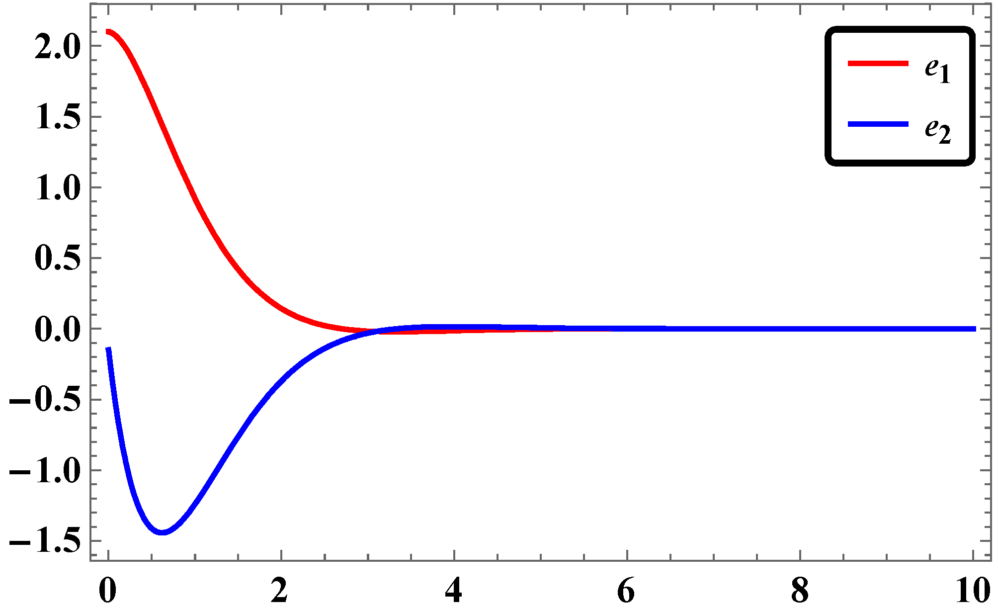
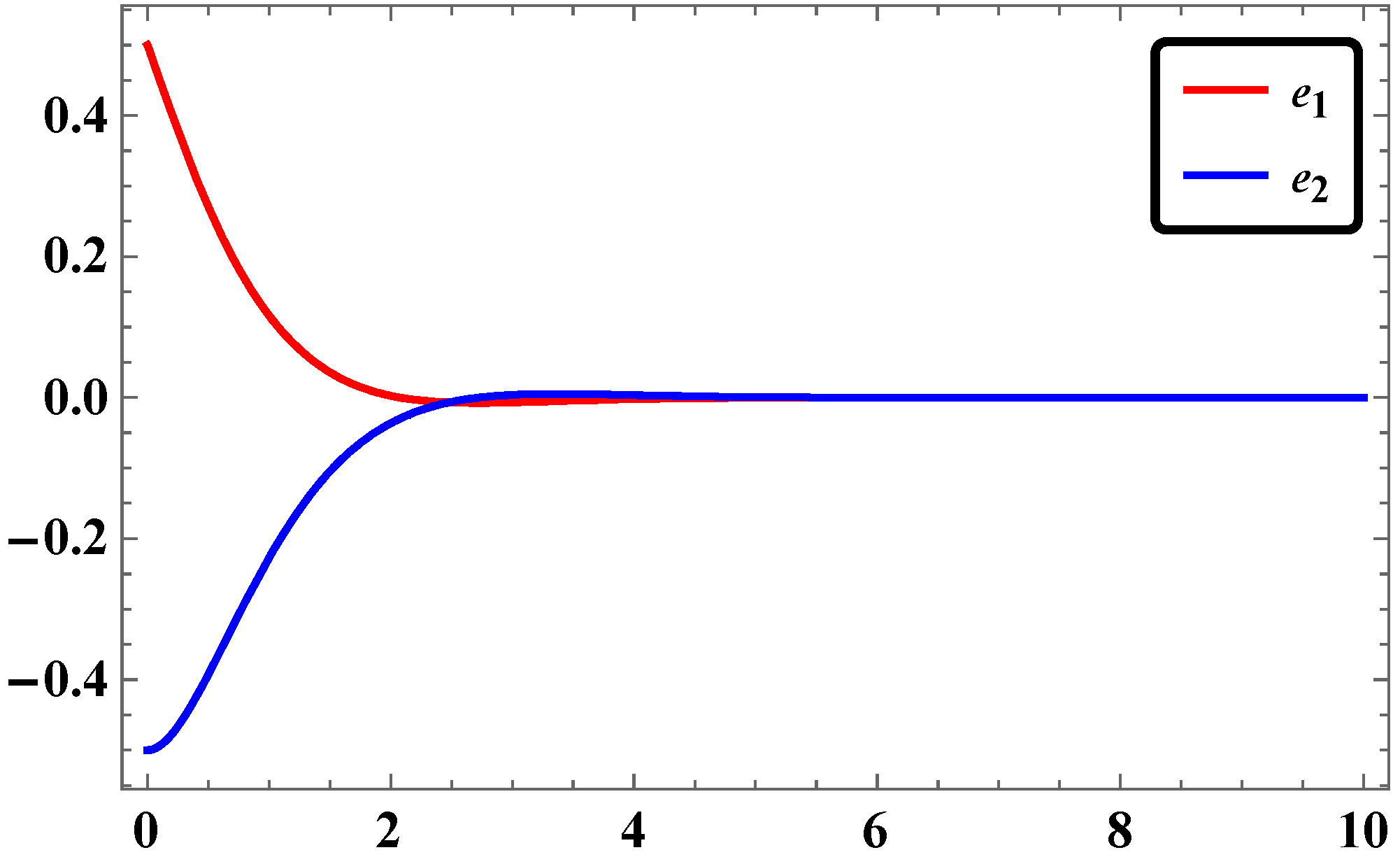
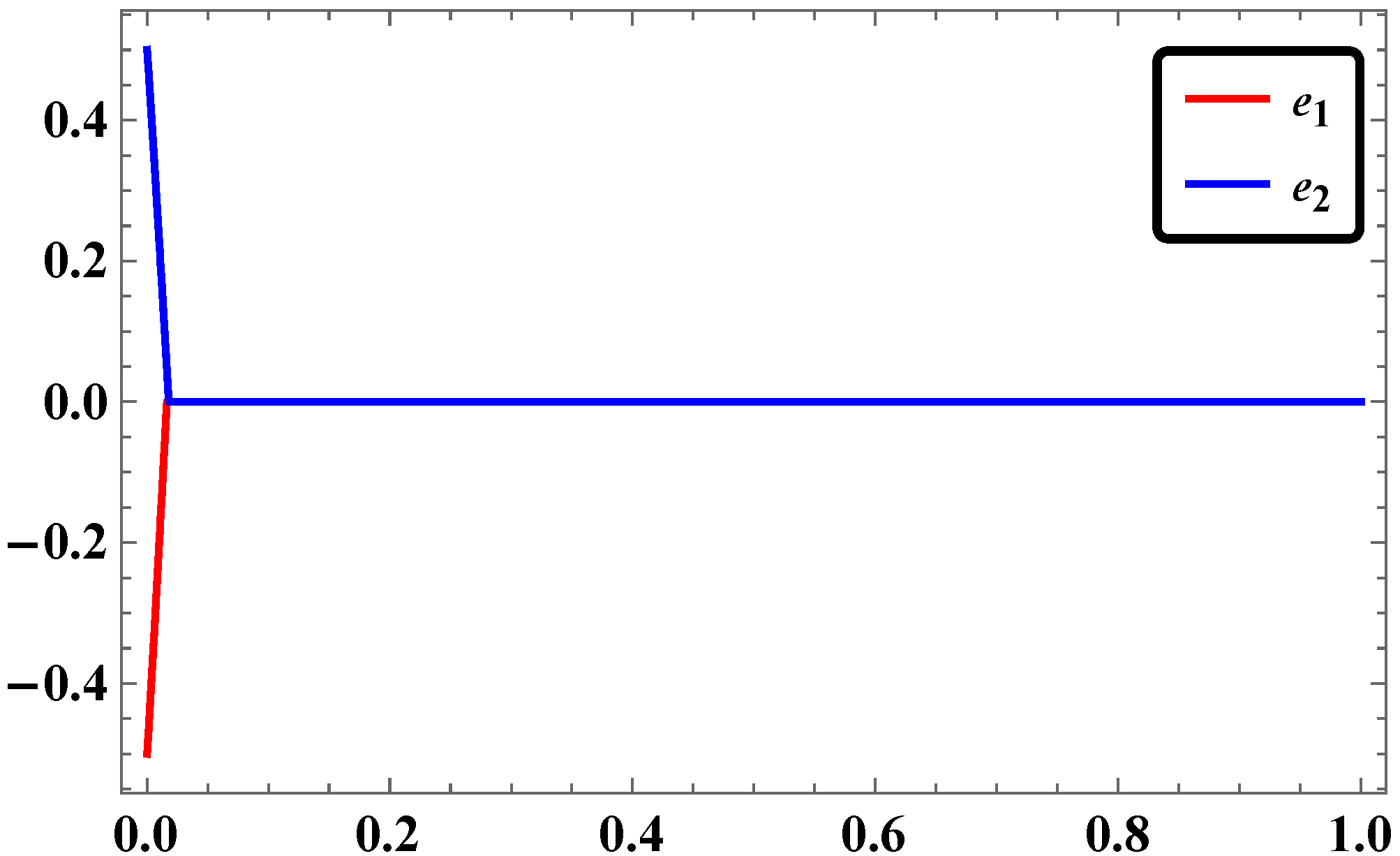
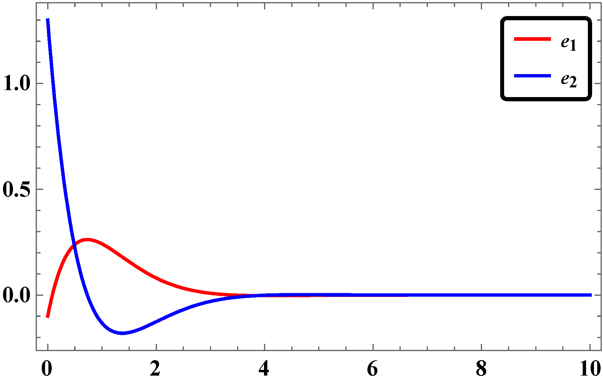
The time response of stabilization of synchronization for LAC in our study was found to occur with rapid convergence if simulation is done with Mathematica.
(2)
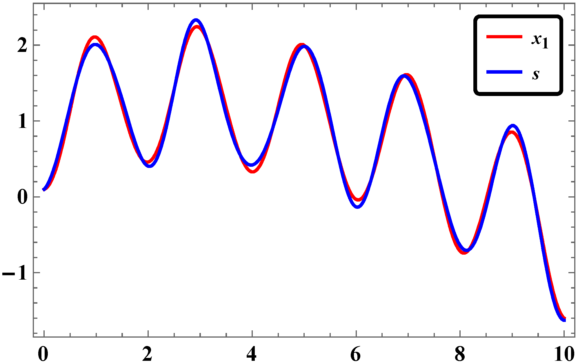
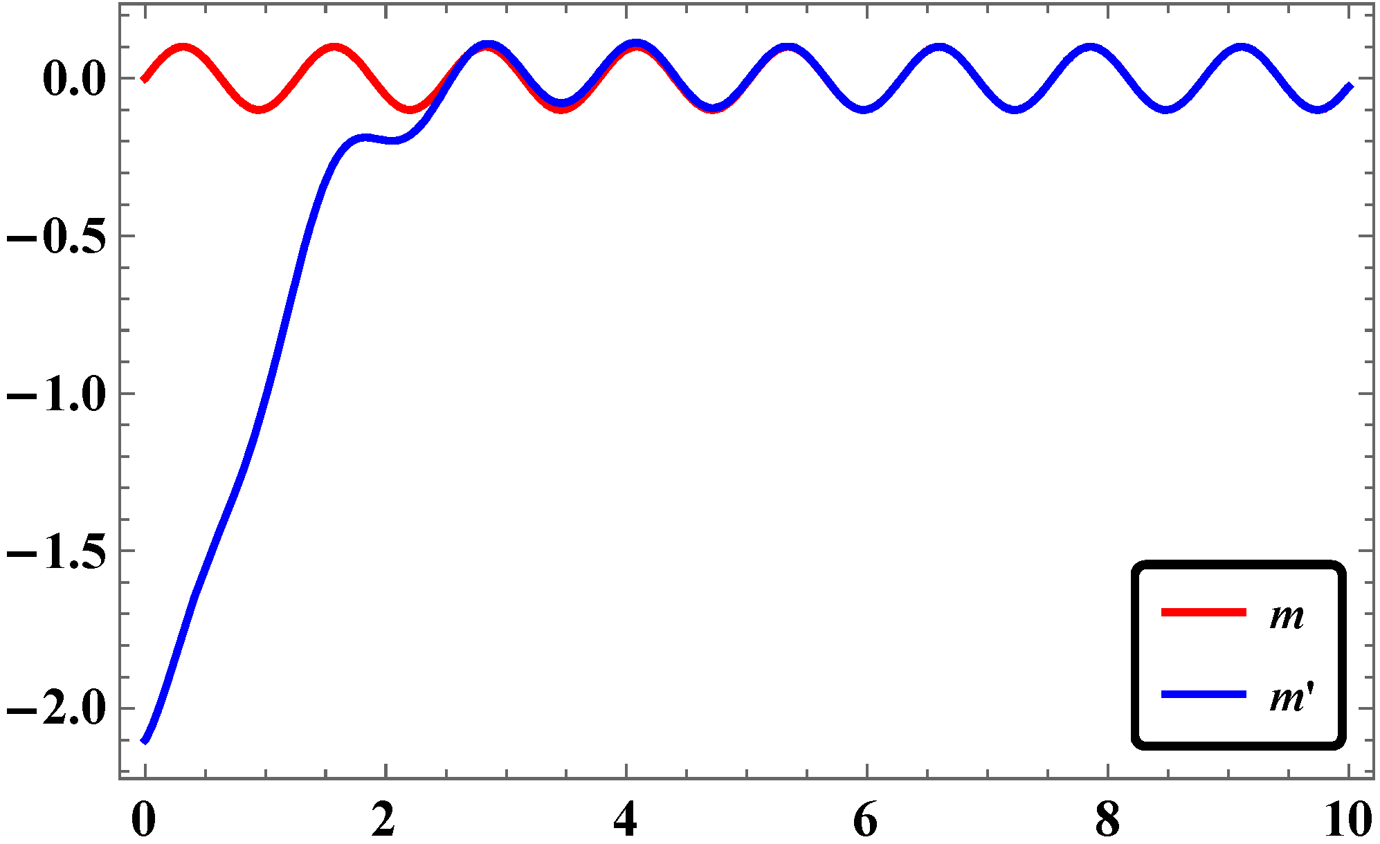
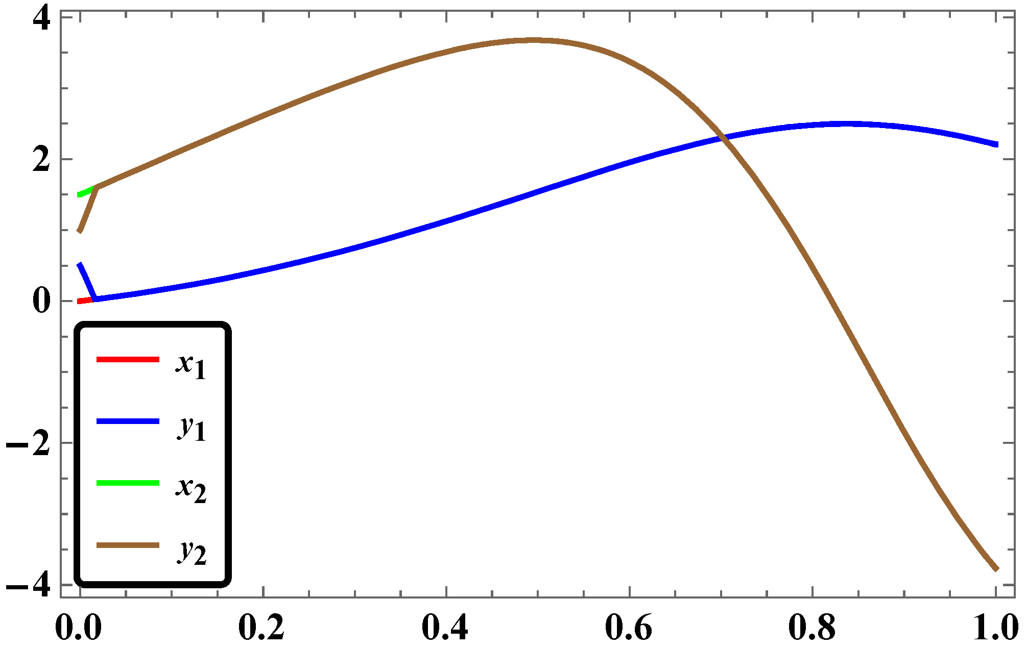
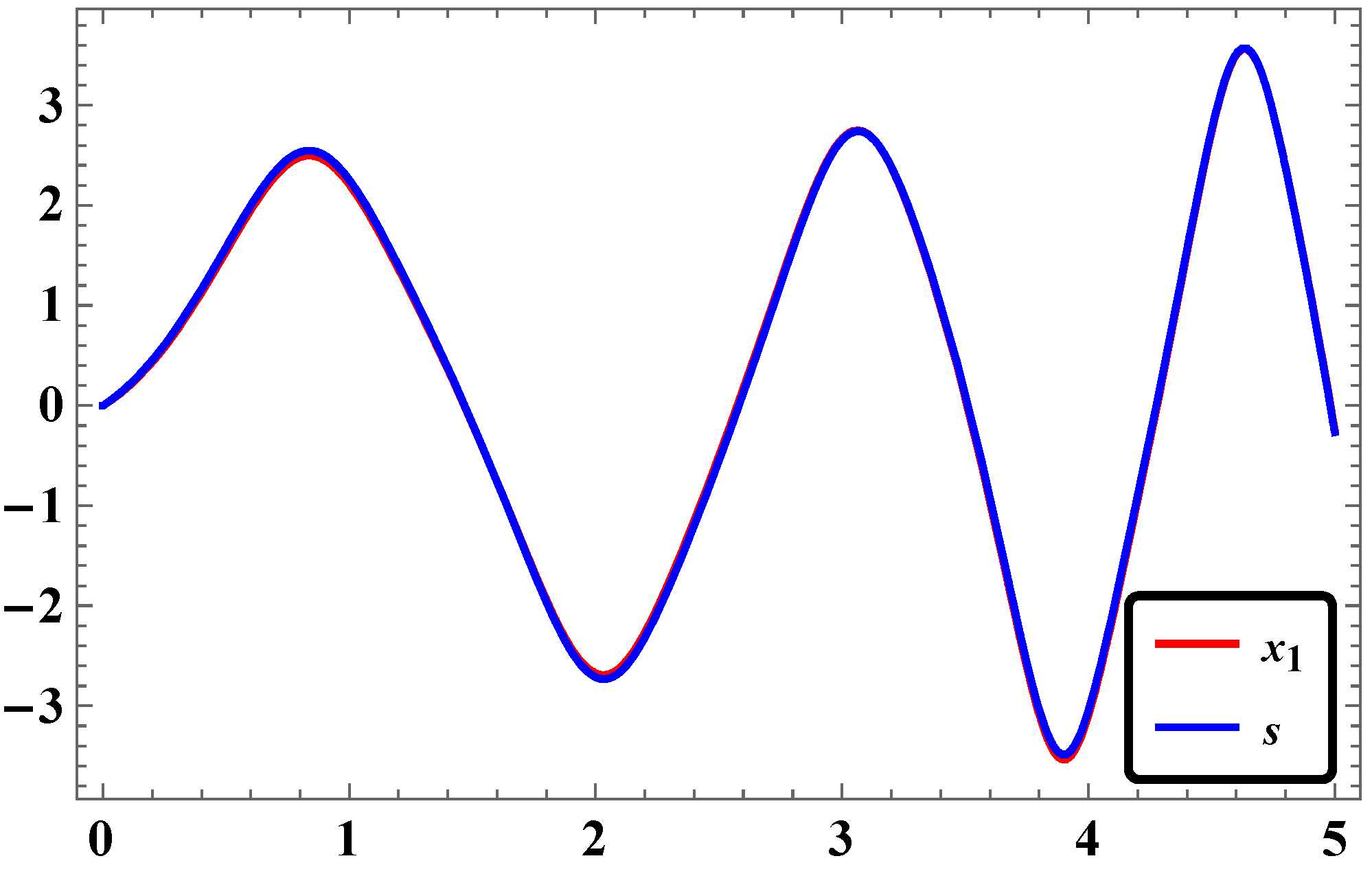
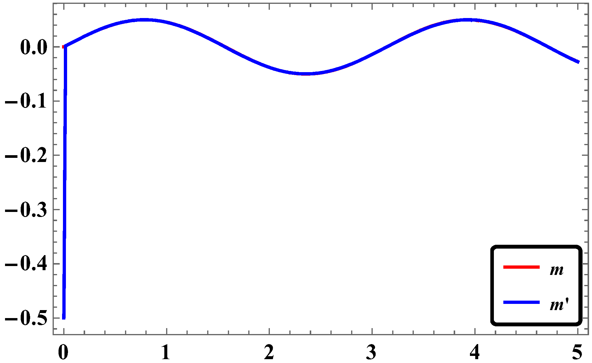
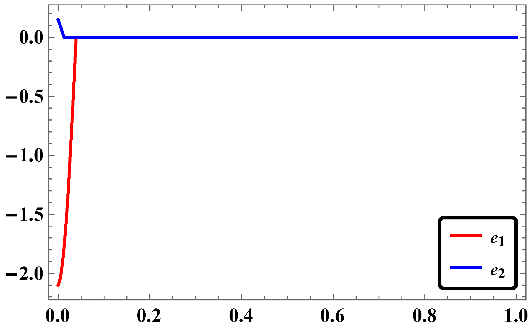
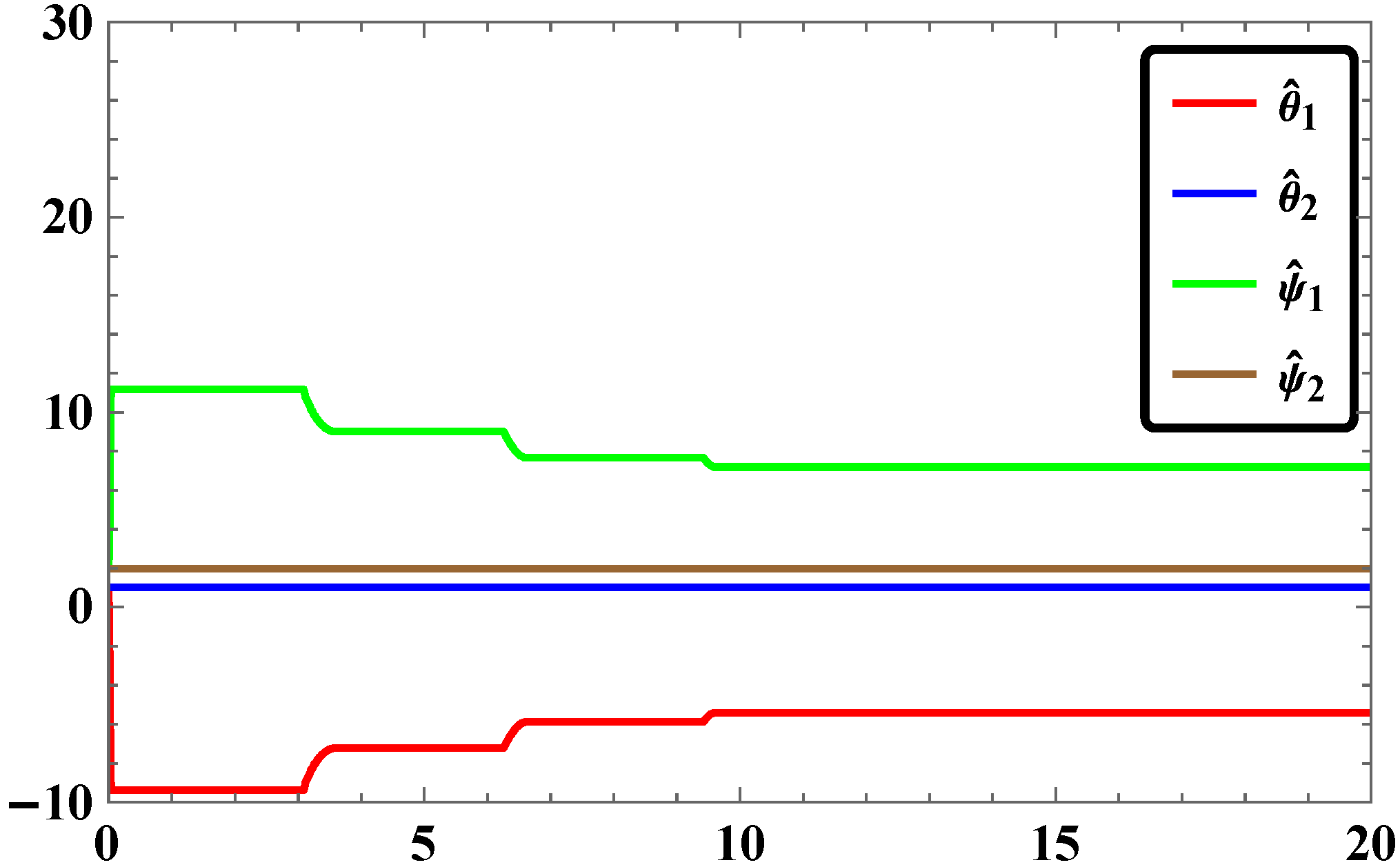
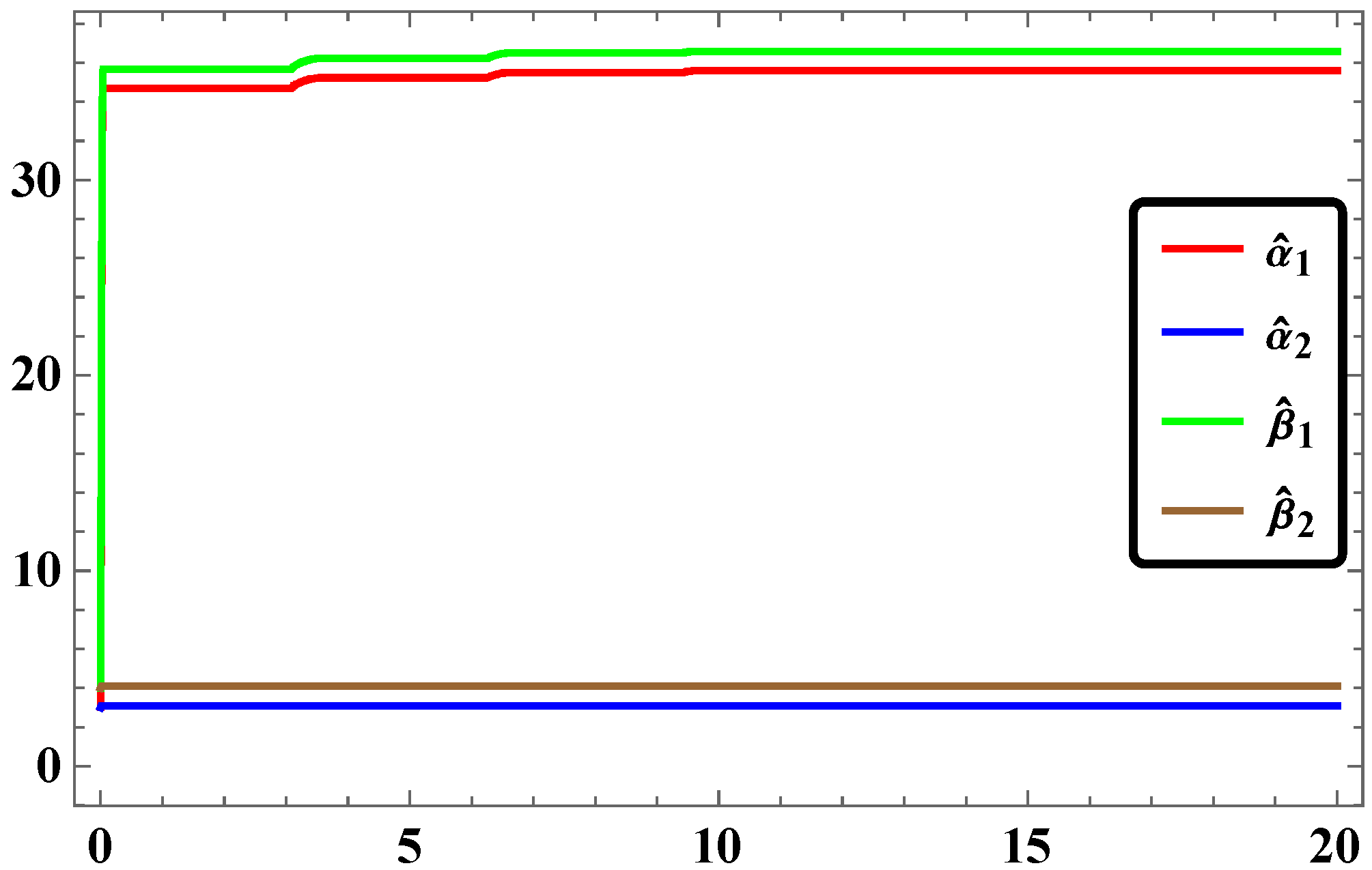
For the same pairs of master and slave systems considered in our study, the RASMC is found to be more effective in terms of time response of stabilization of synchronization.
On the basis of these two points, we conclude that selection of appropriate mathematical tools for simulation and technique for synchronization is very important.

Acknowledgments

The authors would like to express their gratitude to the honorable reviewers who suggested many worthwhile changes to improve the work of this manuscript.

Author Contributions

Azizan Bin Saaban performed the literature review and proposed the problem. Adyda Binti Ibrahin and Israr Ahmad performed the analytical analysis and wrote the paper. Mohammad Shahzad performed the numerical simulations and revised the manuscript.

Conflicts of Interest

The authors declare no conflict of interest.

References

  1. Shahzad, M.; Pham, V.T.; Ahmad, M.A.; Jafari, S.; Hadaeghi, F. Synchronization and circuit design of a chaotic system with coexisting hidden attractors. Eur. Phys. J. Spec. Top. 2015, 224, 1637–1652. [Google Scholar] [CrossRef]
  2. Yao, L.; Cai, G. Chaos Synchronization of a New Hyperchaotic Finance System Via a Novel Chatter Free Sliding Mode Control Strategy. Int. J. Nonlinear Sci. 2014, 17, 176–181. [Google Scholar]
  3. Mobayen, S. A Novel Global Sliding Mode Control Based on Exponential Reaching Law for a Class of under Actuated Systems with External Disturbances. J. Comput. Nonlinear Dyn. 2015, 11, 021011–021019. [Google Scholar] [CrossRef]
  4. Azar, A.T.; Zhu, Q. Advances and Applications in Sliding Mode Control Systems; Springer International Publishing: Cham, Switzerland, 2014. [Google Scholar]
  5. Shahzad, M.; Raziuddin, M. Synchronization Of Three Dimensional Cancer Model With Rosslar System Using A Robust Adaptive Sliding Mode Controller. Int. J. Math. Arch. 2015, 6, 123–132. [Google Scholar]
  6. Shahzad, M.; Saaban, A.B.; Ibrahim, A.B.; Ahmad, I. Adaptive control to synchronise and anti-synchronise two identical time delay Bhalekar-Gejji chaotic systems with unknown parameters. Int. J. Autom. Control 2015, 9, 211–227. [Google Scholar] [CrossRef]
  7. Ma, J.; Zhang, A.; Xia, Y.; Zhang, L. Optimize design of adaptive synchronization controllers and parameter observers in different hyperchaotic systems. Appl. Math. Comput. 2010, 215, 3318–3326. [Google Scholar] [CrossRef]
  8. Lin, C.; Peng, Y.; Lin, M. CMAC-based adaptive backstepping synchronization of uncertain chaotic systems. Chaos Soliton Fract. 2009, 42, 981–988. [Google Scholar] [CrossRef]
  9. Bai, E.W.; Lonngren, K.E. Synchronization of two Lorenz system using Active control. Phys. Rev. Lett. 1997, 64, 1199–1196. [Google Scholar] [CrossRef]
  10. Vincent, U.E. Synchronization of Identical and Nonidentical 4-D Chaotic Systems using Active Control. Chaos Solitons Fract. 2008, 37, 1065–1075. [Google Scholar] [CrossRef]
  11. Njah, A.N. Synchronization and Anti-synchronization of double hump Duffing-Van der Pol Oscillators via Active Control. J. Inf. Comput. Sci. 2009, 4, 243–250. [Google Scholar]
  12. Njah, A.N. Synchronization via active control of parametrically and externally excited Φ6—Van der Pol and duffing oscillators and application to secure communications. J. Vib. Cont. 2011, 17, 493–504. [Google Scholar] [CrossRef]
  13. Shahzad, M.; Ahmad, I. Experimental study of synchronization & Anti-synchronization for spin orbit problem of Enceladus. Int. J. of Cont. Sci. Eng. 2013, 3, 41–47. [Google Scholar]
  14. Pisarchik, A.N.; Arecchi, F.T.; Meucci, R.; Garbo, A.D. Synchronization of Shilnikov Chaos in CO2 Laser with Feedback. Laser Phys. 2014, 11, 1235–1239. [Google Scholar]
  15. Hammami, S. State feedback-based secure image cryptosystem hyperchaotic synchronization. ISA Trans. 2015. [Google Scholar] [CrossRef] [PubMed]
  16. Rafikov, M.; Balthazar, J.M. On control and synchronization in chaotic and hyperchaotic systems via linear feedback control. Commun. Nonlinear Sci. Numer. Simul. 2008, 13, 1246–1255. [Google Scholar] [CrossRef]
  17. Luo, R.Z.; Zhang, F. Finite-Time Modified Projective Synchronization of Unknown Rossler and Coullet Systems. Commun. Control Sci. Eng. 2013, 1, 51–56. [Google Scholar]
  18. Cai, N.; Jing, Y.; Zhang, S. Modified projective synchronization of chaotic systems with disturbances via active sliding mode control. Commun. Nonlinear Sci. Numer. Simul. 2010, 15, 1613–1620. [Google Scholar] [CrossRef]
  19. Fu, G. Robust adaptive modified function projective synchronization of different hyperchaotic systems subject to external disturbance. Commun. Nonlinear Sci. Numer. Simul. 2012, 17, 2602–2608. [Google Scholar] [CrossRef]
  20. Ahmad, I.; Saaban, A.; Ibrahim, A.; Shahzad, M. A Research on the Synchronization of Two Novel Chaotic Systems Based on a Nonlinear Active Control Algorithm. Eng. Tech. Appl. Sci. Res. 2015, 5, 739–747. [Google Scholar]
  21. Singh, P.P.; Singh, J.P.; Roy, B.K. Synchronization and anti-synchronization of Lu and bhalekar-Gejji chaotic systems using nonlinear active control. Chaos Solitons Fract. 2014, 69, 31–39. [Google Scholar] [CrossRef]
  22. Ahmad, I.; Saaban, A.B.; Ibrahim, A.B.; Shahzad, M. On Globally Exponential Stable Complete Synchronization of Nearly Identical Hyperchaotic Systems via Linear Active Control. Ciênc. Téc. Vitiviníc. Sci. Technol. J. 2015, 30, 141–154. [Google Scholar]
  23. Shahzad, M. The Improved Results with Mathematica and Effects of External Uncertainty & Disturbances on Synchronization using a Robust Adaptive Sliding Mode Controller: A Comparative Study. Nonlinear Dyn. 2015, 79, 2037–2054. [Google Scholar]
  24. Pourmahmood, M.; Khanmohammadi, S.; Alizadeh, G. Synchronization of two different uncertain chaotic systems with unknown parameters using a robust adaptive sliding mode controller. Commun. Nonlinear Sci. Numer. Simul. 2011, 16, 2853–2868. [Google Scholar] [CrossRef]
  25. Vaidyanathan, S.; Rasappan, S. Global Chaos Synchronization for WINDMI and Coullet Chaotic Systems Using Active Control. J. Cont. Eng. Tech. 2013, 3, 69–75. [Google Scholar]
  26. Ahmad, I.; Saaban, A.B.; Ibrahim, A.B.; Shahzad, M. A Research on Active Control to Synchronize a New 3D Chaotic System. Systems 2016, 4. [Google Scholar] [CrossRef]
  27. Ahmad, I.; Saaban, A.B.; Ibrahim, A.B.; Shahzad, M.; Naveed, N. The Synchronization of Chaotic Systems with Different Dimensions by a Robust Generalized Active Control. Int. J. Light Electron. Opt. 2016, 127, 4859–4871. [Google Scholar] [CrossRef]
  28. Ahmad, I.; Saaban, A.; Ibrahim, A.; Shahzad, M. Global Chaos Identical and Nonidentical Synchronization of a New Chaotic System Using Linear Active Control. Complexity 2014. [Google Scholar] [CrossRef]
  29. Siewe, S.M.; Moukam, K.F.M.; Tchawoua, C.; Woafo, P. Bifurcation and chaos in triple-well Φ6—Van der Pol oscillator driven by external and parametric excitations. Phys. A 2005, 357, 383–396. [Google Scholar] [CrossRef]
  30. Tchoukuegno, R.; Nbendjo, B.R.N.; Woafo, P. Resonant oscillations and fractal basin boundaries of a particle in a Φ6 potential. Phys. A 2002, 304, 362–368. [Google Scholar] [CrossRef]
  31. Tchoukuegno, R.; Nbendjo, B.R.N.; Woafo, P. Linear feedback and parametric controls of vibrations and chaotic escape in a Φ6 potential. Int. J. Nonlinear Mech. 2003, 38, 531–541. [Google Scholar] [CrossRef]
  32. Li, W.; Chang, K. Robust synchronization of drive-response chaotic systems via adaptive sliding mode control. Chaos Soliton Fract. 2009, 39, 2086–2092. [Google Scholar] [CrossRef]
  33. Yan, J.; Hung, M.; Chiang, T.; Yang, Y. Robust synchronization of chaotic systems via adaptive sliding mode control. Phys. Lett. A 2006, 356, 220–225. [Google Scholar] [CrossRef]
  34. Aghababa, M.P.; Heydari, A. Chaos synchronization between two different chaotic systems with uncertainties, external disturbances, unknown parameters and input nonlinearities. Appl. Math. Model. 2012, 36, 1639–1652. [Google Scholar] [CrossRef]
  35. Aghababa, M.P.; Akbari, M.E. A chattering-free robust adaptive sliding mode controller for synchronization of two different chaotic systems with unknown uncertainties and external disturbances. Appl. Math. Comput. 2012, 218, 5757–5768. [Google Scholar] [CrossRef]
  36. Khan, A.; Shahzad, M. Synchronization of circular restricted three body problem with Lorenz hyper chaotic system using a robust adaptive sliding mode controller. Complexity 2013, 18, 58–64. [Google Scholar] [CrossRef]
Figure 1. Time Series of e 1  &  e 2 .
Systems 04 00025 g001
Figure 2. Time Series of x 1 , y 1 , x 2  &  y 2 .
Systems 04 00025 g002
Figure 3. Time Series of x 1  &  s .
Systems 04 00025 g003
Figure 4. Time Series of m  &  m .
Systems 04 00025 g004
Figure 5. Time Series of e 1  &  e 2 .
Systems 04 00025 g005
Figure 6. Time Series of x 1 , y 1 , x 2  &  y 2 .
Systems 04 00025 g006
Figure 7. Time Series of x 1  &  s .
Systems 04 00025 g007
Figure 8. Time Series of m  &  m .
Systems 04 00025 g008
Figure 9. Time Series of e 1  &  e 2 .
Systems 04 00025 g009
Figure 10. Time Series of x 1 , y 1 , x 2  &  y 2 .
Systems 04 00025 g010
Figure 11. Time Series of x 1  &  s .
Systems 04 00025 g011
Figure 12. Time Series of m  &  m .
Systems 04 00025 g012
Figure 13. Time Series of e.
Systems 04 00025 g013
Figure 14. Time Series of e 1  &  e 2 .
Systems 04 00025 g014
Figure 15. Time Series of θ ^ 1 , θ ^ 2 , ψ ^ 1  &  ψ ^ 2 .
Systems 04 00025 g015
Figure 16. Time Series of α ^ 1 , α ^ 2 , β ^ 1  &  β ^ 2 .
Systems 04 00025 g016
Figure 17. Time Series of x 1 , y 1 , x 2  &  y 2 .
Systems 04 00025 g017
Figure 18. Time Series of x 1  &  s .
Systems 04 00025 g018
Figure 19. Time Series of m  &  m .
Systems 04 00025 g019
Figure 20. Time Series of e 1  &  e 2 .
Systems 04 00025 g020
Figure 21. Time Series of θ ^ 1 , θ ^ 2 , ψ ^ 1  &  ψ ^ 2 .
Systems 04 00025 g021
Figure 22. Time Series of α ^ 1 , α ^ 2 , β ^ 1  &  β ^ 2 .
Systems 04 00025 g022
Figure 23. Time Series of x 1 , y 1 , x 2  &  y 2 .
Systems 04 00025 g023
Figure 24. Time Series of x 1  &  s .
Systems 04 00025 g024
Figure 25. Time Series of m  &  m .
Systems 04 00025 g025
Figure 26. Time Series of e 1  &  e 2 .
Systems 04 00025 g026
Figure 27. Time Series of θ ^ 1 , θ ^ 2 , ψ ^ 1  &  ψ ^ 2 .
Systems 04 00025 g027
Figure 28. Time Series of α ^ 1 , α ^ 2 , β ^ 1  &  β ^ 2 .
Systems 04 00025 g028
Figure 29. Time Series of x 1 , y 1 , x 2  &  y 2 .
Systems 04 00025 g029
Figure 30. Time Series of x 1  &  s .
Systems 04 00025 g030
Figure 31. Time Series of m  &  m .
Systems 04 00025 g031
Figure 32. Time Series of V ˙ ( t ) in all cases.
Systems 04 00025 g032

