
A Hierarchical Aggregation Approach for Indicators Based on Data Envelopment Analysis and Analytic Hierarchy Process

Abstract
:1. Introduction
2. Methodology
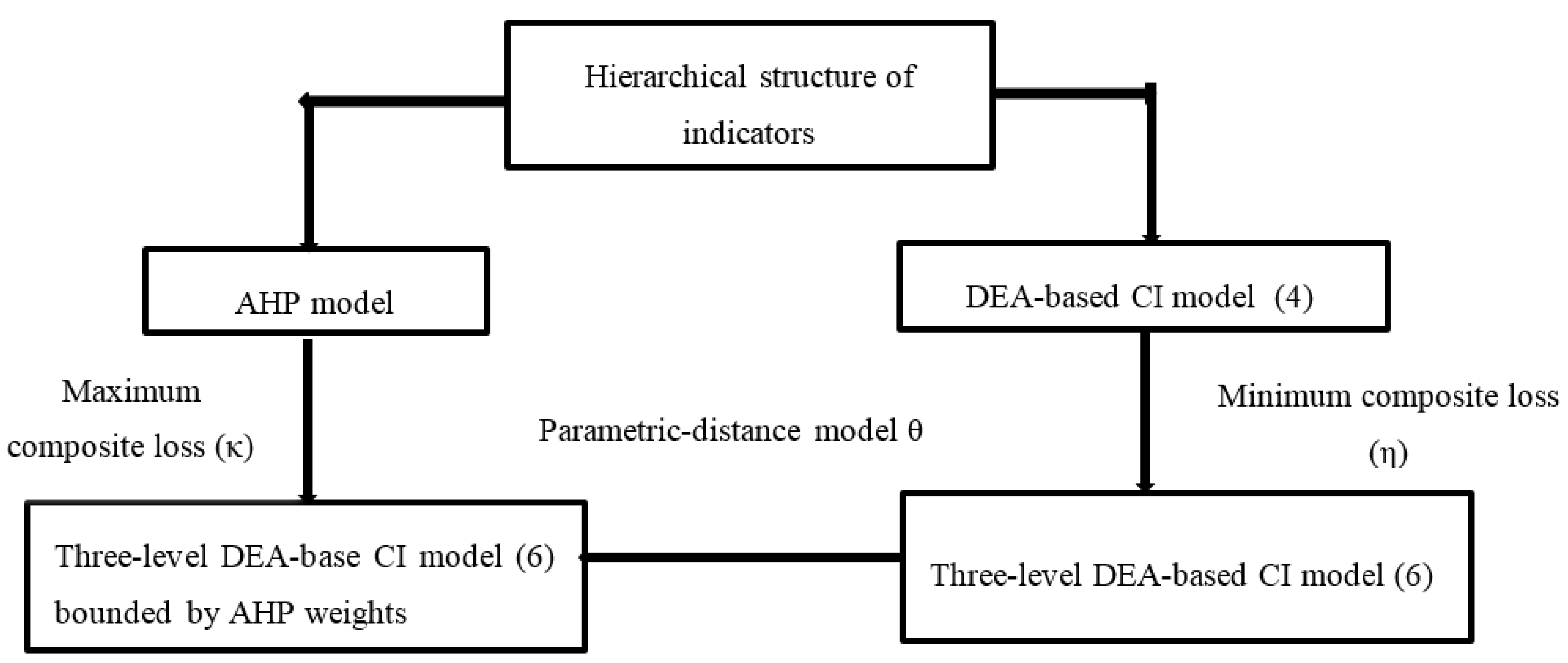
- Computing the composite value of each DMU using one-level DEA-based CI model (4). The computed composite values are applied in three-level DEA-based CI model (6).
- Computing the priority weights of indicators for all DMUs using AHP, which impose weight bounds into model (6).
- Obtaining an optimal set of weights for each DMU using three-level DEA-based CI model (6) (minimum composite loss η).
- Obtaining an optimal set of weights for each DMU using model (6) bounded by AHP (maximum composite loss κ). Note that if the AHP weights are added to model (6), we obtain model (10).
- Measuring the performance of each DMU in terms of the relative closeness to the priority weights of indicators. For this purpose, we develop parameter-distance model (11). Increasing a parameter in a defined range of composite loss we explore how much a DM can achieve its goals. This may result in various ranking positions for a DMU in comparison to the other DMUs.
2.1. DEA-Based CI Model
2.2. Three-Level DEA-Based CI Model
2.3. Prioritizing Indicator Weights Using AHP
2.4. A Parametric Distance Model
3. A Numerical Example: Road Safety Performance Indicators

| Countries | Alcohol | Speed | Protective Systems | ||||||||
|---|---|---|---|---|---|---|---|---|---|---|---|
| % of Drivers above Legal Alcohol Limit In Roadside Police Tests | % of Alcohol Related Fatalities | Mean Speed | Speed Limit Violation (%) | Seat Belt | Child Restraint | ||||||
| Motorways | Rural Roads | Urban Roads | Motorways | Rural Roads | Urban Roads | Daytime Seatbelt Wearing Rate in Front Seats of Light Vehicles (%) | Daytime Seatbelt Wearing Rate in Rear Seats of Light Vehicles (%) | Daytime Usage Rate of Child Restraints (%) | |||
| AUT | 0.116 | 0.463 | 0.938 | 0.781 | 0.802 | 0.766 | 0.051 | 0.254 | 0.904 | 0.699 | 0.863 |
| BEL | 0.068 | 0.654 | 0.846 | 0.743 | 0.768 | 0.348 | 0.029 | 0.222 | 0.799 | 0.488 | 0.729 |
| FIN | 0.593 | 0.136 | 0.963 | 0.729 | 0.907 | 0.409 | 0.023 | 0.323 | 0.911 | 0.922 | 0.716 |
| FRA | 0.263 | 0.123 | 0.933 | 0.787 | 0.838 | 0.505 | 0.037 | 0.318 | 1.000 | 1.000 | 0.937 |
| HUN | 0.279 | 0.283 | 0.955 | 0.793 | 0.817 | 0.362 | 0.033 | 0.230 | 0.727 | 0.501 | 0.433 |
| IRL | 0.237 | 0.119 | 0.945 | 0.762 | 0.724 | 1.000 | 0.032 | 0.223 | 0.901 | 0.914 | 0.857 |
| LTU | 0.555 | 0.321 | 1.000 | 0.713 | 0.714 | 0789 | 0.025 | 0.318 | 0.609 | 0.366 | 0.404 |
| NLD | 0.081 | 1.000 | 0.899 | 0.740 | 0.881 | 0.454 | 0.020 | 0.234 | 0.959 | 0.890 | 0.758 |
| POL | 0.091 | 0.438 | 0.806 | 0.697 | 0.647 | 0.290 | 0.015 | 0.165 | 0.799 | 0.589 | 0.905 |
| PRT | 0.137 | 0.610 | 0.847 | 0.618 | 0.919 | 0.302 | 0.014 | 0.360 | 0.881 | 0.574 | 0.591 |
| SVN | 0.122 | 0.078 | 0.964 | 1.000 | 0.713 | 0.480 | 1.000 | 0.163 | 0.874 | 0.551 | 0.672 |
| SWE | 1.000 | 0.357 | 0.883 | 0.717 | 0.870 | 0.241 | 0.019 | 0.259 | 0.973 | 0.927 | 1.000 |
| CHE | 0.277 | 0.230 | 0.943 | 0.757 | 1.000 | 0.710 | 0.043 | 1.000 | 0.887 | 0.805 | 0.895 |
| Objective Level | Criteria Level | Sub-Criteria Level | Sub-Sub-Criteria Level |
|---|---|---|---|
| Prioritizing road user behavior | Alcohol 0.2727 | % of drivers above legal alcohol limit 0.333 | % of drivers above legal alcohol limit 1.000 |
| % of alcohol-related fatalities 0.667 | % of alcohol-related fatalities 1.000 | ||
| Speed 0.5454 | Mean speed 0.60 | Mean speed of vehicles on motorways 0.081 | |
| Mean speed of vehicles on rural roads, 0.342 | |||
| Mean speed of vehicles on urban roads, 0.577 | |||
| Speed limit violations 0.40 | % of vehicles exceeding the speed limit on motorways 0.081 | ||
| % of vehicles exceeding the speed limit on rural roads 0.342 | |||
| % of vehicles exceeding the speed limit on urban roads 0.577 | |||
| Protective systems 0.1818 | Seat belt 0.40 | Daytime seatbelt wearing rate in front seats of light vehicles (%) 0.60 | |
| Daytime seatbelt wearing rate in rear seats of light vehicles (%) 0.40 | |||
| Child Restraint 0.60 | Daytime usage rate of child restraints (%) 1.000 |
| Weights of Categories | Weights of Sub-Categories | Weights of Sub-Sub-Categories |
|---|---|---|
| 0.0361 | 0.0000 | 0.0000 |
| 0.0361 | 0.0361 | |
| 0.9415 | 0.9415 | 0.9415 |
| 0.0000 | ||
| 0.0000 | ||
| 0.0000 | 0.0000 | |
| 0.0000 | ||
| 0.0000 | ||
| 0.1160 | 0.0000 | 0.0000 |
| 0.0000 | ||
| 0.1160 | 0.1160 | |
| Countries | η | κ | |
|---|---|---|---|
| AUT | 1.000 | 0.000 | 0.158 |
| BEL | 0.938 | 0.000 | 0.127 |
| FIN | 1.000 | 0.000 | 0.173 |
| FRA | 1.000 | 0.000 | 0.184 |
| HUN | 1.000 | 0.000 | 0.284 |
| IRL | 1.000 | 0.000 | 0.254 |
| LTU | 1.000 | 0.000 | 0.270 |
| NLD | 1.000 | 0.000 | 0.023 |
| POL | 0.955 | 0.000 | 0.224 |
| PRT | 0.978 | 0.000 | 0.139 |
| SVN | 1.000 | 0.000 | 0.208 |
| SWE | 1.000 | 0.000 | 0.040 |
| CHE | 1.000 | 0.000 | 0.000 |
| Weights of Categories | Weights of Sub-Categories | Weights of Sub-Sub-Categories |
|---|---|---|
| 0.4089 | 0.1362 | 0.1362 |
| 0.2727 | 0.2727 | |
| 0.8178 | 0.4907 | 0.0397 |
| 0.1678 | ||
| 0.2831 | ||
| 0.3271 | 0.0265 | |
| 0.1119 | ||
| 0.1888 | ||
| 0.2726 | 0.1090 | 0.0654 |
| 0.0436 | ||
| 0.1636 | 0.1636 | |
| 1.4993 | ||
| Countries | Rank | |
|---|---|---|
| AUT | 0.332 | 6 |
| BEL | 0.705 | 11 |
| FIN | 0.438 | 9 |
| FRA | 0.338 | 7 |
| HUN | 0.591 | 10 |
| IRL | 0.331 | 5 |
| LTU | 0.381 | 8 |
| NLD | 0.021 | 2 |
| POL | 0.718 | 12 |
| PRT | 0.782 | 13 |
| SVN | 0.166 | 4 |
| SWE | 0.035 | 3 |
| CHE | 0.000 | 1 |

4. Conclusions
Conflicts of Interest
Appendix A
| θ | AUT | BEL | FIN | FRA | HUN | IRL | LTU | NLD | POL | PRT | SVN | SWE | CHE |
|---|---|---|---|---|---|---|---|---|---|---|---|---|---|
| 0 | 0.0000 | 0.0000 | 0.0000 | 0.0000 | 0.0000 | 0.0000 | 0.0000 | 0.0000 | 0.0000 | 0.0000 | 0.0000 | 0.0000 | 1.0000 |
| Rank | N/A | N/A | N/A | N/A | N/A | N/A | N/A | N/A | N/A | N/A | N/A | N/A | 1 |
| 0.01 | 0.0788 | 0.3002 | 0.0808 | 0.0595 | 0.0784 | 0.0450 | 0.0419 | 0.4367 | 0.1951 | 0.2454 | 0.0492 | 0.2521 | 1.0000 |
| Rank | 8 | 3 | 7 | 10 | 9 | 12 | 13 | 2 | 6 | 5 | 11 | 4 | 1 |
| 0.02 | 0.1479 | 0.4018 | 0.1497 | 0.1190 | 0.1295 | 0.0863 | 0.0823 | 0.8733 | 0.2640 | 0.3572 | 0.0983 | 0.5041 | 1.0000 |
| Rank | 8 | 4 | 7 | 10 | 9 | 12 | 13 | 2 | 6 | 5 | 11 | 3 | 1 |
| 0.03 | 0.2160 | 0.4852 | 0.2148 | 0.1784 | 0.1793 | 0.1269 | 0.1223 | 1.0000 | 0.3268 | 0.4286 | 0.1473 | 0.7562 | 1.0000 |
| Rank | 7 | 4 | 8 | 10 | 9 | 12 | 13 | 1 | 6 | 5 | 11 | 3 | 1 |
| 0.04 | 0.2838 | 0.5605 | 0.2797 | 0.2378 | 0.2272 | 0.1675 | 0.1624 | 1.0000 | 0.3845 | 0.5133 | 0.1963 | 1.0000 | 1.0000 |
| Rank | 7 | 4 | 8 | 9 | 10 | 12 | 13 | 1 | 6 | 5 | 11 | 1 | 1 |
| 0.05 | 0.3512 | 0.6312 | 0.3444 | 0.2970 | 0.2679 | 0.2081 | 0.2023 | 1.0000 | 0.4418 | 0.5846 | 0.2452 | 1.0000 | 1.0000 |
| Rank | 7 | 4 | 8 | 9 | 10 | 12 | 13 | 1 | 6 | 5 | 11 | 1 | 1 |
| 0.06 | 0.4185 | 0.7113 | 0.4091 | 0.3562 | 0.3073 | 0.2486 | 0.2422 | 1.0000 | 0.4832 | 0.6491 | 0.2941 | 1.0000 | 1.0000 |
| Rank | 7 | 4 | 8 | 9 | 10 | 12 | 13 | 1 | 6 | 5 | 11 | 1 | 1 |
| 0.07 | 0.4857 | 0.7813 | 0.4736 | 0.4152 | 0.3454 | 0.2891 | 0.2819 | 1.0000 | 0.5195 | 0.7121 | 0.3428 | 1.0000 | 1.0000 |
| Rank | 7 | 4 | 8 | 9 | 10 | 12 | 13 | 1 | 6 | 5 | 11 | 1 | 1 |
| 0.08 | 0.5527 | 0.8464 | 0.5379 | 0.4740 | 0.3818 | 0.3296 | 0.3215 | 1.0000 | 0.5556 | 0.7739 | 0.3913 | 1.0000 | 1.0000 |
| Rank | 7 | 4 | 8 | 9 | 11 | 12 | 13 | 1 | 6 | 5 | 10 | 1 | 1 |
| 0.09 | 0.6196 | 0.8991 | 0.6019 | 0.5325 | 0.4163 | 0.3699 | 0.3609 | 1.0000 | 0.5915 | 0.8331 | 0.4397 | 1.0000 | 1.0000 |
| Rank | 6 | 4 | 7 | 9 | 11 | 12 | 13 | 1 | 8 | 5 | 10 | 1 | 1 |
| 0.1 | 0.6861 | 0.9396 | 0.6655 | 0.5906 | 0.4497 | 0.4102 | 0.4001 | 1.0000 | 0.6273 | 0.8858 | 0.4879 | 1.0000 | 1.0000 |
| Rank | 6 | 4 | 7 | 9 | 11 | 12 | 13 | 1 | 8 | 5 | 10 | 1 | 1 |
| 0.11 | 0.7520 | 0.9692 | 0.7283 | 0.6481 | 0.4829 | 0.4504 | 0.4391 | 1.0000 | 0.6628 | 0.9290 | 0.5358 | 1.0000 | 1.0000 |
| Rank | 6 | 4 | 7 | 9 | 11 | 12 | 13 | 1 | 8 | 5 | 10 | 1 | 1 |
| 0.12 | 0.8166 | 0.9869 | 0.7896 | 0.7046 | 0.5160 | 0.4905 | 0.4778 | 1.0000 | 0.6980 | 0.9645 | 0.5833 | 1.0000 | 1.0000 |
| Rank | 6 | 4 | 7 | 8 | 11 | 12 | 13 | 1 | 9 | 5 | 10 | 1 | 1 |
| 0.13 | 0.8777 | 1.0000 | 0.8476 | 0.7596 | 0.5490 | 0.5304 | 0.5161 | 1.0000 | 0.7328 | 0.9838 | 0.6309 | 1.0000 | 1.0000 |
| Rank | 14 | 1 | 15 | 16 | 19 | 20 | 21 | 1 | 17 | 11 | 18 | 1 | 1 |
| 0.14 | 0.9271 | 1.0000 | 0.8967 | 0.8115 | 0.5818 | 0.5701 | 0.5540 | 1.0000 | 0.7669 | 1.0000 | 0.6784 | 1.0000 | 1.0000 |
| Rank | 14 | 1 | 15 | 16 | 19 | 20 | 21 | 1 | 17 | 1 | 18 | 1 | 1 |
| 0.15 | 0.9681 | 1.0000 | 0.9289 | 0.8577 | 0.6145 | 0.6096 | 0.5913 | 1.0000 | 0.8007 | 1.0000 | 0.7260 | 1.0000 | 1.0000 |
| Rank | 14 | 1 | 15 | 16 | 19 | 20 | 21 | 1 | 17 | 1 | 18 | 1 | 1 |
| 0.16 | 1.0000 | 1.0000 | 0.9592 | 0.8998 | 0.6468 | 0.6489 | 0.6279 | 1.0000 | 0.8340 | 1.0000 | 0.7735 | 1.0000 | 1.0000 |
| Rank | 14 | 1 | 15 | 16 | 20 | 19 | 21 | 1 | 17 | 1 | 18 | 1 | 1 |
| 0.17 | 1.0000 | 1.0000 | 0.9896 | 0.9409 | 0.6789 | 0.6880 | 0.6635 | 1.0000 | 0.8665 | 1.0000 | 0.8211 | 1.0000 | 1.0000 |
| Rank | 1 | 1 | 7 | 8 | 12 | 11 | 13 | 1 | 9 | 1 | 10 | 1 | 1 |
| 0.18 | 1.0000 | 1.0000 | 1.0000 | 0.9820 | 0.7104 | 0.7269 | 0.6987 | 1.0000 | 0.8973 | 1.0000 | 0.8687 | 1.0000 | 1.0000 |
| Rank | 1 | 1 | 1 | 8 | 12 | 11 | 13 | 1 | 9 | 1 | 10 | 1 | 1 |
| 0.19 | 1.0000 | 1.0000 | 1.0000 | 1.0000 | 0.7415 | 0.7655 | 0.7335 | 1.0000 | 0.9253 | 1.0000 | 0.9162 | 1.0000 | 1.0000 |
| Rank | 1 | 1 | 1 | 1 | 12 | 11 | 13 | 1 | 9 | 1 | 10 | 1 | 1 |
| 0.2 | 1.0000 | 1.0000 | 1.0000 | 1.0000 | 0.7724 | 0.8036 | 0.7677 | 1.0000 | 0.9538 | 1.0000 | 0.9638 | 1.0000 | 1.0000 |
| Rank | 1 | 1 | 1 | 1 | 12 | 11 | 13 | 1 | 10 | 1 | 9 | 1 | 1 |
| 0.21 | 1.0000 | 1.0000 | 1.0000 | 1.0000 | 0.8029 | 0.8408 | 0.8015 | 1.0000 | 0.9736 | 1.0000 | 1.0000 | 1.0000 | 1.0000 |
| Rank | 1 | 1 | 1 | 1 | 12 | 11 | 13 | 1 | 10 | 1 | 1 | 1 | 1 |
| 0.22 | 1.0000 | 1.0000 | 1.0000 | 1.0000 | 0.8329 | 0.8772 | 0.8349 | 1.0000 | 0.9919 | 1.0000 | 1.0000 | 1.0000 | 1.0000 |
| Rank | 1 | 1 | 1 | 1 | 13 | 11 | 12 | 1 | 10 | 1 | 1 | 1 | 1 |
| 0.23 | 1.0000 | 1.0000 | 1.0000 | 1.0000 | 0.8621 | 0.9136 | 0.8681 | 1.0000 | 1.0000 | 1.0000 | 1.0000 | 1.0000 | 1.0000 |
| Rank | 1 | 1 | 1 | 1 | 13 | 11 | 12 | 1 | 1 | 1 | 1 | 1 | 1 |
| 0.24 | 1.0000 | 1.0000 | 1.0000 | 1.0000 | 0.8905 | 0.9501 | 0.9013 | 1.0000 | 1.0000 | 1.0000 | 1.0000 | 1.0000 | 1.0000 |
| Rank | 1 | 1 | 1 | 1 | 13 | 11 | 12 | 1 | 1 | 1 | 1 | 1 | 1 |
| 0.25 | 1.0000 | 1.0000 | 1.0000 | 1.0000 | 0.9180 | 0.9865 | 0.9345 | 1.0000 | 1.0000 | 1.0000 | 1.0000 | 1.0000 | 1.0000 |
| Rank | 1 | 1 | 1 | 1 | 13 | 11 | 12 | 1 | 1 | 1 | 1 | 1 | 1 |
| 0.26 | 1.0000 | 1.0000 | 1.0000 | 1.0000 | 0.9432 | 1.0000 | 0.9677 | 1.0000 | 1.0000 | 1.0000 | 1.0000 | 1.0000 | 1.0000 |
| Rank | 1 | 1 | 1 | 1 | 13 | 1 | 12 | 1 | 1 | 1 | 1 | 1 | 1 |
| 0.27 | 1.0000 | 1.0000 | 1.0000 | 1.0000 | 0.9669 | 1.0000 | 0.9999 | 1.0000 | 1.0000 | 1.0000 | 1.0000 | 1.0000 | 1.0000 |
| Rank | 1 | 1 | 1 | 1 | 13 | 1 | 12 | 1 | 1 | 1 | 1 | 1 | 1 |
| 0.28 | 1.0000 | 1.0000 | 1.0000 | 1.0000 | 0.9906 | 1.0000 | 1.0000 | 1.0000 | 1.0000 | 1.0000 | 1.0000 | 1.0000 | 1.0000 |
| Rank | 1 | 1 | 1 | 1 | 13 | 1 | 1 | 1 | 1 | 1 | 1 | 1 | 1 |
| 0.29 | 1.0000 | 1.0000 | 1.0000 | 1.0000 | 1.0000 | 1.0000 | 1.0000 | 1.0000 | 1.0000 | 1.0000 | 1.0000 | 1.0000 | 1.0000 |
| Rank | 1 | 1 | 1 | 1 | 1 | 1 | 1 | 1 | 1 | 1 | 1 | 1 | 1 |
References
- OECD. Organisation for Economic Co-operation and Development (OECD). In Handbook on Constructing Composite Indicators: Methodology and User Guide; OECD Publishing: Paris, France, 2008. [Google Scholar]
- San Cristobal Mateo, J.R. Multi-Criteria Analysis in the Renewable Energy Industry; Springer: London, UK, 2012. [Google Scholar]
- Ebert, U.; Welsch, H. Meaningful environmental indices: A social choice approach. J. Environ. Econ. Manag. 2004, 47, 270–283. [Google Scholar] [CrossRef]
- Munda, G.; Nardo, M. Noncompensatory/nonlinear composite indicators for ranking countries: A defensible setting. Appl. Econ. 2009, 41, 1513–1523. [Google Scholar] [CrossRef]
- Zhou, P.; Ang, B.W. Comparing MCDA aggregation methods in constructing composite indicators using the Shannon-Spearman measure. Soc. Indic. Res. 2009, 94, 83–96. [Google Scholar] [CrossRef]
- Cooper, W.W.; Seiford, L.M.; Zhu, J. Handbook on Data Envelopment Analysis; Kluwer Academic Publishers: Norwel, MA, USA, 2004. [Google Scholar]
- Chaaban, J.M. Measuring youth development: A nonparametric cross-country “youth welfare index”. Soc. Indic. Res. 2009, 93, 351–358. [Google Scholar] [CrossRef]
- Murias, P.; de Miguel, J.C.; Rodriguez, D. A composite indicator for university quality assessment: The case of Spanish higher education system. Soc. Indic. Res. 2008, 89, 129–146. [Google Scholar] [CrossRef]
- Murias, P.; Martinez, F.; de Miguel, C. An economic wellbeing index for the Spanish provinces: A data envelopment analysis approach. Soc. Indic. Res. 2006, 77, 395–417. [Google Scholar] [CrossRef]
- Cherchye, L.; Moesen, W.; Rogge, N.; van Puyenbroeck, T.; Saisana, M.; Saltelli, A.; Liska, R.; Tarantola, S. Creating composite indicators with DEA and robustness analysis: The case of the technology achievement index. J. Oper. Res. Soc. 2008, 59, 239–251. [Google Scholar] [CrossRef]
- Cherchye, L.; Moesen, W.; Rogge, N.; van Puyenbroeck, T. An introduction to “benefit of the doubt” composite indicators. Soc. Indic. Res. 2007, 82, 111–145. [Google Scholar] [CrossRef]
- Zhou, P.; Ang, B.W.; Poh, K.L. A mathematical programming approach to constructing composite Indicators. Ecol. Econ. 2007, 62, 291–297. [Google Scholar] [CrossRef]
- Arora, A.; Arora, A.S.; Palvia, S. Social media index valuation: Impact of technological, social, economic, and ethical dimensions. J. Promot. Manag. 2014, 20, 328–344. [Google Scholar] [CrossRef]
- Dedeke, N. Estimating the weights of a composite index using AHP: Case of the environmental performance index. Br. J. Arts Soc. Sci. 2013, 11, 199–221. [Google Scholar]
- Singh, R.K.; Murty, H.R.; Gupta, S.K.; Dikshit, A.K. Development of composite sustainability performance index for steel industry. Ecol. Indic. 2007, 7, 565–588. [Google Scholar] [CrossRef]
- Saaty, T.S. The Analytic Hierarchy Process; McGraw-Hill: New York, NY, USA, 1980. [Google Scholar]
- Vaidya, O.S.; Kumar, S. Analytic hierarchy process: An overview of applications. Eur. J. Oper. Res. 2006, 169, 1–29. [Google Scholar] [CrossRef]
- Entani, T.; Ichihashi, H.; Tanaka, H. Evaluation method based on interval AHP and DEA. Cent. Eur. J. Oper. Res. 2004, 12, 25–34. [Google Scholar]
- Kong, W.; Fu, T. Assessing the performance of business colleges in Taiwan using data envelopment analysis and student based value-added performance indicators. Omega 2012, 40, 541–549. [Google Scholar] [CrossRef]
- Lee, A.H.I.; Lin, C.Y.; Kang, H.Y.; Lee, W.H. An integrated performance evaluation model for the photovoltaics industry. Energies 2012, 5, 1271–1291. [Google Scholar] [CrossRef]
- Liu, C.M.; Hsu, H.S.; Wang, S.T.; Lee, H.K. A performance evaluation model based on AHP and DEA. J. Chin. Inst. Ind. Eng. 2005, 22, 243–251. [Google Scholar] [CrossRef]
- Takamura, Y.; Tone, K. A comparative site evaluation study for relocating Japanese government agencies out of Tokyo. Socio-Econ. Plan. Sci. 2003, 37, 85–102. [Google Scholar] [CrossRef]
- Tseng, W.; Yang, C.; Wang, D. Using the DEA and AHP methods on the optimal selection of IT strategic alliance partner. In Proceedings of the 2009 International Conference on Business and Information (BAI 2009), Kuala Lumpur, Malaysia, 23–30 June 2009; Academy of Taiwan Information Systems Research (ATISR): Taipei, Taiwan, 2009; Volume 6, pp. 1–15. [Google Scholar]
- Premachandra, I.M. Controlling factor weights in data envelopment analysis by Incorporating decision maker’s value judgement: An approach based on AHP. J. Inf. Manag. Sci. 2001, 12, 1–12. [Google Scholar]
- Shang, J.; Sueyoshi, T. Theory and Methodology—A unified framework for the selection of a Flexible Manufacturing System. Eur. J. Oper. Res. 1995, 85, 297–315. [Google Scholar]
- Lozano, S.; Villa, G. Multiobjective target setting in data envelopment analysis using AHP. Comput. Oper. Res. 2009, 36, 549–564. [Google Scholar] [CrossRef]
- Azadeh, A.; Ghaderi, S.F.; Izadbakhsh, H. Integration of DEA and AHP with computer simulation for railway system improvement and optimization. Appl. Math. Comput. 2008, 195, 775–785. [Google Scholar] [CrossRef]
- Ertay, T.; Ruan, D.; Tuzkaya, U.R. Integrating data envelopment analysis and analytic hierarchy for the facility layout design in manufacturing systems. Inf. Sci. 2006, 176, 237–262. [Google Scholar] [CrossRef]
- Jyoti, T.; Banwet, D.K.; Deshmukh, S.G. Evaluating performance of national R & D organizations using integrated DEA-AHP technique. Int. J. Product. Perform. Manag. 2008, 57, 370–388. [Google Scholar]
- Korpela, J.; Lehmusvaara, A.; Nisonen, J. Warehouse operator selection by combining AHP and DEA methodologies. Int. J. Product. Econ. 2007, 108, 135–142. [Google Scholar] [CrossRef]
- Lin, M.; Lee, Y.; Ho, T. Applying integrated DEA/AHP to evaluate the economic performance of local governments in china. Eur. J. Oper. Res. 2011, 209, 129–140. [Google Scholar] [CrossRef]
- Ramanathan, R. Supplier selection problem: Integrating DEA with the approaches of total cost of ownership and AHP. Supply Chain Manag. 2007, 12, 258–261. [Google Scholar] [CrossRef]
- Raut, R.D. Environmental performance: A hybrid method for supplier selection using AHP-DEA. Int. J. Bus. Insights Transform. 2011, 5, 16–29. [Google Scholar]
- Yang, T.; Kuo, C. A hierarchical AHP/DEA methodology for the facilities layout design problem. Eur. J. Oper. Res. 2003, 147, 128–136. [Google Scholar] [CrossRef]
- Ho, C.B.; Oh, K.B. Selecting internet company stocks using a combined DEA and AHP approach. Int. J. Syst. Sci. 2010, 41, 325–336. [Google Scholar] [CrossRef]
- Jablonsky, J. Measuring the efficiency of production units by AHP models. Math. Comput. Model. 2007, 46, 1091–1098. [Google Scholar] [CrossRef]
- Sinuany-Stern, Z.; Mehrez, A.; Hadada, Y. An AHP/DEA methodology for ranking decision making units. Int. Trans. Oper. Res. 2000, 7, 109–124. [Google Scholar] [CrossRef]
- Chen, T.Y. Measuring firm performance with DEA and prior information in Taiwan’s banks. Appl. Econ. Lett. 2002, 9, 201–204. [Google Scholar] [CrossRef]
- Cai, Y.; Wu, W. Synthetic financial evaluation by a method of combining DEA with AHP. Int. Trans. Oper. Res. 2001, 8, 603–609. [Google Scholar] [CrossRef]
- Feng, Y.; Lu, H.; Bi, K. An AHP/DEA method for measurement of the efficiency of R & D management activities in universities. Int. Trans. Oper. Res. 2004, 11, 181–191. [Google Scholar]
- Kim, T. Extended Topics in the Integration of Data Envelopment Analysis and the Analytic Hierarchy Process in Decision Making. Ph.D. Thesis, Louisiana State University, Baton Rouge, LA, USA, 2000. [Google Scholar]
- Pakkar, M.S. Using the AHP and DEA methodologies for stock selection. In Business Performance Measurement and Management; Charles, V., Kumar, M., Eds.; Cambridge Scholars Publishing: Newcastle upon Tyne, UK, 2014; pp. 566–580. [Google Scholar]
- Liu, C.; Chen, C. Incorporating value judgments into data envelopment analysis to improve decision quality for organization. J. Am. Acad. Bus. 2004, 5, 423–427. [Google Scholar]
- Saen, R.F.; Memariani, A.; Lotfi, F.H. Determining relative efficiency of slightly non-homogeneous decision making units by data envelopment analysis: A case study in IROST. Appl. Math. Comput. 2005, 165, 313–328. [Google Scholar] [CrossRef]
- Pakkar, M.S. An integrated approach based on DEA and AHP. Comput. Manag. Sci. 2015, 12, 153–169. [Google Scholar] [CrossRef]
- Pakkar, M.S. Using data envelopment analysis and analytic hierarchy process for multiplicative aggregation of financial ratios. J. Appl. Oper. Res. 2015, 7, 23–35. [Google Scholar]
- Pakkar, M.S. Measuring the efficiency and effectiveness of decision making units by integrating the DEA and AHP methodologies. In Business Performance Measurement and Management; Charles, V., Kumar, M., Eds.; Cambridge Scholars Publishing: Newcastle upon Tyne, UK, 2014; pp. 552–565. [Google Scholar]
- Pakkar, M.S. Using DEA and AHP for ratio analysis. Am. J. Oper. Res. 2014, 4, 268–279. [Google Scholar] [CrossRef] [Green Version]
- Pakkar, M.S. Using data envelopment analysis and analytic hierarchy process to construct composite indicators. J. Appl. Oper. Res. 2014, 6, 174–187. [Google Scholar]
- Pakkar, M.S. An integrated approach to the DEA and AHP methodologies in decision making. In Data Envelopment Analysis and Its Applications to Management; Charles, V., Kumar, M., Eds.; Cambridge Scholars Publishing: Newcastle upon Tyne, UK, 2012; pp. 136–149. [Google Scholar]
- Pakkar, M.S. Using DEA and AHP for multiplicative aggregation of indicators. Am. J. Oper. Res. 2015, 5, 327–336. [Google Scholar] [CrossRef]
- Shen, Y.; Hermans, E.; Brijs, T.; Wets, G. Data envelopment analysis for composite indicators: A multiple layer model. Soc. Indic. Res. 2013, 114, 739–756. [Google Scholar] [CrossRef]
- Shen, Y.; Hermans, E.; Ruan, D.; Wets, G.; Brijs, T.; Vanhoof, K. A generalized multiple layer data envelopment analysis model for hierarchical structure assessment: A case study in road safety performance evaluation. Expert Syst. Appl. 2011, 38, 15262–15272. [Google Scholar] [CrossRef]
- Liu, W.B.; Zhang, D.Q.; Meng, W.; Li, X.X.; Xu, F. A study of DEA models without explicit inputs. Omega 2011, 39, 472–480. [Google Scholar] [CrossRef]
- Charnes, A.; Cooper, W.W.; Rhodes, E. Measuring the Efficiency of Decision Making Units. Eur. J. Oper. Res. 1978, 2, 429–444. [Google Scholar] [CrossRef]
- Hashimoto, A.; Wu, D.A. A DEA-compromise programming model for comprehensive ranking. J. Oper. Res. Soc. Jpn. 2004, 47, 73–81. [Google Scholar]
- Mavi, R.K.; Mavi, N.K.; Mavi, L.K. Compromise programming for common weight analysis in data envelopment analysis. Am. J. Sci. Res. 2012, 45, 90–109. [Google Scholar]
- Podinovski, V.V. Suitability and redundancy of non-homogeneous weight restrictions for measuring the relative efficiency in DEA. Eur. J. Oper. Res. 2004, 154, 380–395. [Google Scholar] [CrossRef]
- Romero, C.; Rehman, T. Multiple Criteria Analysis for Agricultural Decisions, 2nd ed.; Elsevier: Amsterdam, The Netherlands, 2003. [Google Scholar]
© 2016 by the author; licensee MDPI, Basel, Switzerland. This article is an open access article distributed under the terms and conditions of the Creative Commons by Attribution (CC-BY) license (http://creativecommons.org/licenses/by/4.0/).
Share and Cite
Pakkar, M.S. A Hierarchical Aggregation Approach for Indicators Based on Data Envelopment Analysis and Analytic Hierarchy Process. Systems 2016, 4, 6. https://doi.org/10.3390/systems4010006
Pakkar MS. A Hierarchical Aggregation Approach for Indicators Based on Data Envelopment Analysis and Analytic Hierarchy Process. Systems. 2016; 4(1):6. https://doi.org/10.3390/systems4010006
Chicago/Turabian StylePakkar, Mohammad Sadegh. 2016. "A Hierarchical Aggregation Approach for Indicators Based on Data Envelopment Analysis and Analytic Hierarchy Process" Systems 4, no. 1: 6. https://doi.org/10.3390/systems4010006
APA StylePakkar, M. S. (2016). A Hierarchical Aggregation Approach for Indicators Based on Data Envelopment Analysis and Analytic Hierarchy Process. Systems, 4(1), 6. https://doi.org/10.3390/systems4010006