Abstract
This work addresses the spread of a disease within an urban system, defined as a network of interconnected cities. The first step consists of comparing two different approaches: a macroscopic one, based on a system of coupled Ordinary Differential Equations (ODE) Susceptible-Infected-Recovered (SIR) systems exploiting populations on nodes and flows on edges (so-called metapopulational model), and a hybrid one, coupling ODE SIR systems on nodes and agents traveling on edges. Under homogeneous conditions (mean field approximation), this comparison leads to similar results on the outputs on which we focus (the maximum intensity of the epidemic, its duration and the time of the epidemic peak). However, when it comes to setting up epidemic control strategies, results rapidly diverge between the two approaches, and it appears that the full macroscopic model is not completely adapted to these questions. In this paper, we focus on some control strategies, which are quarantine, avoidance and risk culture, to explore the differences, advantages and disadvantages of the two models and discuss the importance of being hybrid when modeling and simulating epidemic spread at the level of a whole urban system.
1. Introduction
Dynamic modeling of city systems often involves coupling processes at different temporal and spatial scales. Single scalar models, whether completely aggregated at the macroscopic scale or completely disaggregated at the microscopic level, are struggling to reach these goals. Yet, the dynamic coupling of networks is often a common point of these two families of approaches. The spatial and temporal coherence of these models at different scales is therefore an important issue. As such, the modeling of the spread of epidemics in structured populations is a particularly active area of application that we propose to retain as a basis here. We will focus more specifically on the intercity spread of infectious diseases via an air network. The aim is to systematically compare two different formalizations of the same problem: one, described as “metapopulation”, is based on an aggregate deterministic modeling of coupled urban epidemic dynamics, while the other is stochastic and combines aggregated and agent-based modeling.
The first approach, metapopulation, comes from research in ecology [1,2] and then was applied to various fields, especially in models examining the spread of diseases within networks [2,3,4,5]. This formalism allows handling very large populations that are spatially distributed. Corresponding models are mainly used to study the conditions for the spread of a disease and to test different control strategies or behavioral adaptations [5].
The second approach aims to overcome the limitations inherent to the first one, including heterogeneous populations and behaviors, and is arguably more adapted when it comes to integrating the intentionality, reflexivity and adaptability of humans in the model [6,7,8].
To our knowledge, only a few works [9] mobilize and compare these two approaches. Papers focusing on agent-based models insist more on the comparison between individual-based models and equation-based models (e.g., to estimate the parameters of the equations from the dynamics generated by individuals’ interactions [7,10]).
However, when studying social phenomena, as in an urban context, such couplings may be required. This is the case, for example, once a background dynamics must be introduced forming the evolving context in which individuals or groups of individuals interact. Handling spatial and temporal coherence of the models at different scales is an important issue, as well as the systematic exploration of the properties of hybrid models [5]. Indeed, model coupling brings out a number of fundamental problems, such as: (1) the preservation of a population during transfers between the macroscale (rational numbers) and microscale (whole numbers); (2) the inclusion of a population considered as homogeneous in the aggregated model components and of heterogeneous individuals in its disaggregated components; (3) the articulation of different scales of time and space, handling for example the spread of an epidemic at a city level and the traveling behavior of individuals; and (4) the characterization of the behavior of the global model and its properties, which cannot be reduced to the properties of each of its components.
In this work, the epidemic dynamics is modeled, in each city, with an SIR (Susceptible- Infected-Recovered) model [11]. Mobility between cities is introduced in an aggregated (metapopulation model called Metapop) and disaggregated (agent based model, called MicMac) manner. In both cases, we are therefore dealing with coupled SIR on spatial networks.
The article is organized as follows. Section 2 introduces the two main kinds of epidemic spread models in a spatial network. Section 3 proposes a first baseline comparison between the two modeling approaches. Section 4 proposes to calibrate time and space over parameter values and explores both the impacts of flight duration and the network topology over results. Mitigation strategies are introduced in Section 5, and Section 6 concludes.
2. Modeling Epidemic Spread in a Spatial Network
We consider the case of a directed and weighted graph composed of nodes. A node is a city, and an edge represents an aerial link between two nodes.
2.1. The SIR Model
A SIR model, describing the evolution of the number of healthy (S), infected (I) and immune (R) people in a population, is given by the system Equation (1) [11,12].
Each city owns a population composed of three distinct groups: susceptible (S), infected (I) and recovered (R). In this simple model, demography is not taken into account, and therefore, population is constant (). Transfer from susceptible to infected is given by the term , where is the contagion rate in the presence of contacts between susceptible and infected people. The passage of infected to recovered depends on , the proportion of infected people healing at every time step. Therefore, denotes the average infectious period of infectious individuals.
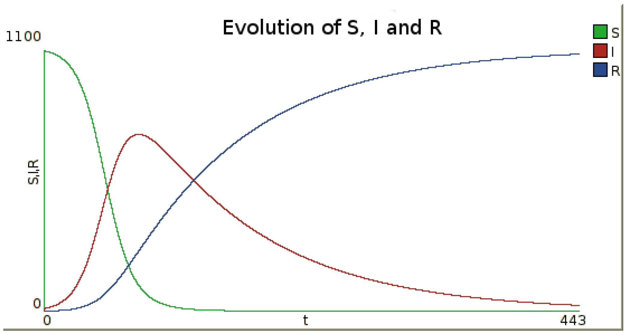
The possible behavior of such a model is shown on Figure 1, on which time series evolution of the numbers of susceptible (S), infected (I) and recovered (R) are presented. These results are obtained using the numerical integration method Runge–Kutta 4
In the remaining paragraphs, each city will be identified by an index , and the population of city i () is denoted by and is therefore composed of , and (with ).

Figure 1.
Example of the evolution of the number of susceptible, infected and recovered inhabitants in time for one node. To obtain this figure, a simulation was performed with the infection rate and the recovery rate , leading to the basic reproduction number . Initial numbers of susceptible, infected and recovered are , and . The numerical integration method is Runge–Kutta 4, with a step.
2.2. Coupling SIR Models on a Network
We now add edges representing flight connections between cities. We also define a mobility rate () representing, for each city i, the proportion of outgoing travelers. This proportion may be different depending on each specific group (S, I or R). In this case, the mobility rate is respectively given by , and . The mobile population of the city i is then given by or by if the mobility rate differs according to each infectious state.
Once mobility rates are defined, travelers leaving a city will be able to head to adjacent cities. We propose in the sequel two approaches in order to account for this mobility component.
2.3. Metapopulation Approach
The metapopulation approach (see [2,3]) considers the network as a directed and weighted network (composed of nodes and edges, along which a population moves). Edges are weighted with a value , representing the fraction of outgoing population from node i pointing to incoming node j. By construction, the following constraint applies: with and if there is no edge from i to j.
This approach assumes trips to be instantaneous (as if Euclidean distance between two cities were zero) and computes the intercity traveler flows at each simulation step. Since this model is by nature atemporal, the time elapsed during the simulation can only be expressed in terms of integration step (without any regard to the real time scale).
The complete model consists of the following system of equations:
For each node, the epidemic dynamics takes into account outgoing (e.g., for susceptible) and incoming (e.g., for susceptible) populations. Note that global population remains constant during the simulation. Figure 2 illustrates the interface of this metapopulation model.
In the following, this model is called “MetaPop, for “Metapopulation”.

Figure 2.
Interface of the metapopulation model, through which the user selects the network topology and mobility rates, as well as the initial population distribution ((left) side of the interface). Typical outputs are computed and displayed during the simulation, such as the numbers of susceptible (S), infected (I) and recovered (R) at each time step (called here a “tick”) or at the end of the simulation, such as “epidemic duration” ((right) side of the interface). (Central) map displays the network of cities and their evolution in terms of number of Infected, during the simulation.

2.4. Hybrid Micro-Macro Approach
The previous approach, while presenting some advantages, also suffers from severe limitations, especially concerning its mobility component, handled as it is in an aggregate way. We propose here an alternative discrete approach, fully disaggregated: travelers, their number depending on the mobility rate, flying between cities, are extracted as discrete entities from their outgoing city S, I, R stocks and are added to their destination city S, I, R stocks. Travelers are carried using a new entity, aircraft, which thus contains an integer stock of susceptible, infected and recovered travelers. Space and time can then be calibrated, as flight duration depends on intercity distance, as a first approximation. Such a simple analogy involves however a prior calibration step, as flight durations need to be synchronized with the numerical integration steps of cities’ SIR models. Preserving a constant population is not straightforward anymore, as the model combines a discrete (mobility) and a continuous (SIR) component, and thus, such a hybrid model needs to be carefully implemented.
The interface of this hybrid model called “MicMac” (for “Micro-Macro”) , presented in more details in [13], is introduced in Figure 3.
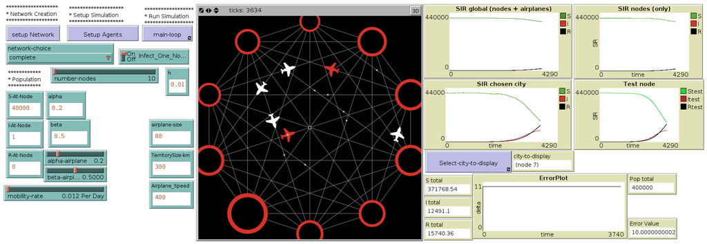
Figure 3.
Interface of the micro-macro hybrid model, through which the user selects the network topology, the mobility rates and the initial population distributions ((left) side of the interface). At each time step, the difference between the total population in the network and the original population is calculated and plotted (“error plot”, (right) side of the interface). (Central) map displays the network of cities, their evolution in terms of number of Infected as well as flights occurring during the simulation (red airplanes contain at least one infected).

One of the main anticipated advantages of this hybrid model, overwhelming its increase in complexity compared to the metapopulation one, resides in its capacity to relax the hypothesis of instantaneous intercity trips. Indeed, during the flights, within the aircraft, the spread of the disease continues, as traveling agents may become infected or recovered. Thus, at each time step, the model updates S, I, R values not only in cities, but also in aircraft. This “while flying” epidemic dynamics is handled also by SIR models, thus leading to a very large number of coupled city and aircraft SIR models (a discrete stochastic approach (Gillespie) was also implemented for the within aircraft epidemic dynamics, but without providing significant differences in model outputs, while largely increasing the computation time).
3. Mean Field Approximation as a Baseline
As a first milestone for comparing these two models, we provide here a mean field approximation of the epidemic dynamics, under the following assumptions: let us consider a complete network (each city is connected to every other city via a directed edge), a constant mobility rate g and constant edge weights , as well as a fixed number of cities and a fixed number N of inhabitants for each city.
In order to compare these models, we introduce the following indicators:
- the maximum value of infected people ();
- the time at which this value is reached ();
- the duration of the epidemic (), that is the time to reach the condition that the number of infected people is below a small epsilon.
Analytically, we can compute the first indicator () for a set of identical nodes as follows. This value is given by:
Indeed, the maximum value of I for a single node (thus, a single simple SIR model), , is obtained for , i.e., for .
Moreover, we can compute:
Integrating this equation along S gives:
At initialization, we have and , which gives:
Since is reached for , the theoretical maximum value of I (), is given by:
Then, in a set of identical nodes, the :
The corresponding values for and duration are obtained by simulation (Figure 4).
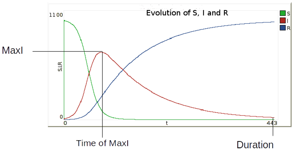
Figure 4.
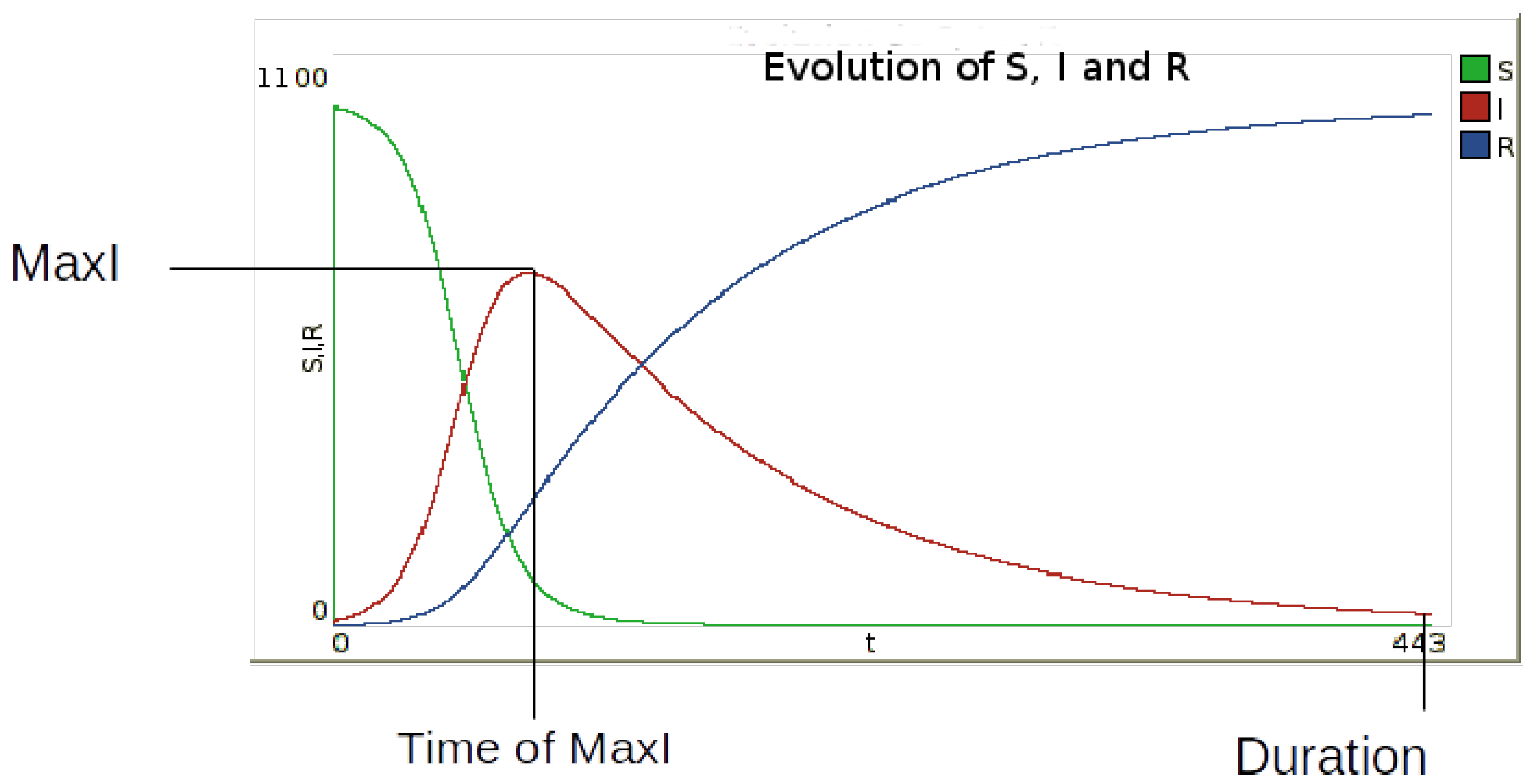
Identification of the three output indicators defined to describe the epidemic dynamics: (maximum number of infected persons), (the time at which this value is reached) and epidemic .
Figure 4.
Identification of the three output indicators defined to describe the epidemic dynamics: (maximum number of infected persons), (the time at which this value is reached) and epidemic .
We have then verified the capacity of the two models to reproduce exactly these three theoretical parameters, under the equivalent conditions. For the MetaPop model, the parallel is quite obvious: a complete directed network, with equivalent initial conditions for every node, equivalent weights for every edge and a fixed mobility rate. For the hybrid MicMac model, while network characteristics are strictly equivalent, considering instantaneous trips implies reducing to zero the distance between the nodes.
An important point needs to be highlighted here: if the initial number of infected persons per node is uniform, then both the MetaPop and MicMac models produce the same three outputs. However, if we introduce one infected person only () and localize him or her randomly on a single node, then we obtain by simulation the following relations:
- of MetaPop > of MicMac
- of MetaPop < of MicMac
- of MetaPop < of MicMac
This divergence is important, as it illustrates a major issue when modeling a contagion process with a continuous and a discrete approach: in MetaPop (continuous), after one iteration, every node is infected from the first infected node, while in MicMac (discrete regarding its mobility component), it can eventually take a number of iterations before every node is infected.
4. Calibrating Time and Space
4.1. Experimental Conditions
As a basis for comparison, we define the experimental conditions in Table 1; unless otherwise stated, they will be used in each of the following simulations.

Table 1.
Experimental conditions.
| Parameter | Value | Parameter | Value |
|---|---|---|---|
| 30 nodes | N | 40,000 people /nodes | |
| α | 0.2 | β | 0.5 |
| Mobility rate g | 0.12 | Territory size | 300 km2 |
| Aircraft capacity | 80 passengers | Initial number of infected people | 1 randomly localized |
| Network topology | Complete |
The number of nodes and their initial size define an acceptable computational burden, given the number of simulations to be run. The values of epidemic parameters are chosen such that the reproduction number () matches the one observed for flu (). This reproduction number corresponds to the number of infected people due to a single initial infected person. Therefore, if , the infection will spread, while if , the infection will die out (it may be noted, however, that given the stochasticity of the agent-based component, infected agents may not be able to spread the disease through the network, for example if the mobility rate is low or if a containment strategy is applied (see Section 5); in such cases, the epidemic will be limited to one or a few nodes and will then indeed die out). These values of α and β are often used when it comes to the study of the SIR model. The mobility rate corresponds to a very active system (as described from U.S. data on domestic flights (see [14])), while territory size and aircraft size were chosen as reasonable values when comparing our experimental setup to U.S. characteristics.
4.2. Impact of Traveling Distance in MicMac
From this basis of comparison and in order to assess the impact of intercity distance on epidemic dynamics, we relax the assumption of “instantaneous movement” in the MicMac hybrid model. Introducing a non-zero distance between nodes implies taking into account a temporal coupling between traveling times and integration time.
Before simulation, an SIR model is integrated on a reference node, using parameter values and initial conditions set up by the user. More precisely, this reference node contains the whole population of the model. The number of iterations (based on Runge-Kutta of order 4 method called RK4) needed to run the model on this reference node, the halt condition being reached if the number infected is below a small epsilon, is calculated and compared to the duration of the epidemic, in days, declared by the user. This ratio determines the corresponding “time” of a step. Moreover, territory being incorporated in the model via the network structure, this preliminary operation allows deducing intercity distances, but also determining transportation time (flight durations).
We are then interested in evaluating the influence of traveling distances (and therefore, territory size) on the three indicators defined previously; see Figure 5.
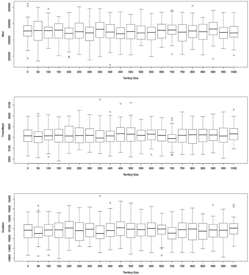
Figure 5.
Impact of traveling distances on epidemic dynamics defined by the three output indicators retained ( in (top), in (middle) and in (below) figures) in MicMac model(number of replications: 50). “Territory size” (in ) displays no significant impact on the values of the three output indicators retained.

Surprisingly, while traveling time increases with territory size, there was no significant impact on the dynamics of the epidemic. In order to make sure the contagion process during flight, formalized as ordinary differential equations, was not the cause, we compared it with a discrete formalism (the so-called Gillespie approach), possibly more adapted to small populations.
4.2.1. Gillespie vs. ODE for Contagion during Flights
In order to determine whether the use of an SIR model during the flights was adequate, we compared its dynamics with a discrete one, for populations ranging from five to 1000 agents.
The Gillespie method is stochastic, aimed at studying homogeneous systems consisting of a small number of entities, using discrete event simulations (see [15,16]). It is based on an analogy with chemical processes, within which a reaction between two entities can occur with a certain probability when they interact during a randomly-defined step time τ. In this specific case, the Gillespie algorithm can be described as follows:
- We initialize stocks S, I and R.
- We setup the list of possible events. In the SIR model, a susceptible person can become infected, and infected people can recover. Therefore, there are two possible reactions, infection and recovery, given by the following expressions: and . Both reactions can be broken down as follows:
- We define as a random number between zero and one. We calculate the time before the next event: .
- We define as a random number between zero and one. The event occurring after time τ is contagion if and healing otherwise.
- We update the values of S, I and R and repeat the previous steps.
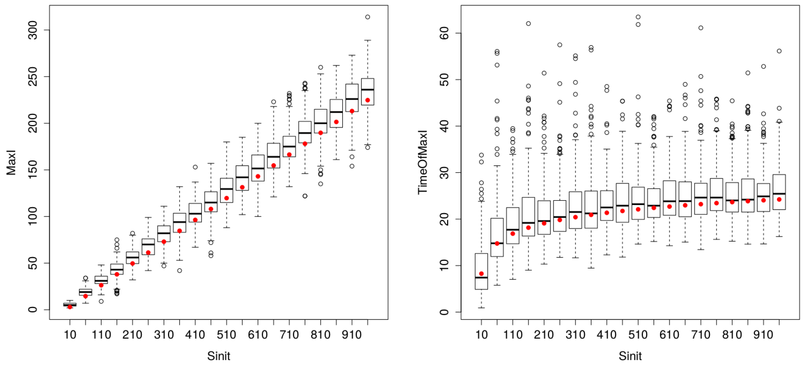
As shown in Figure 6, both formalisms (ODE and Gillespie) provide very close estimates, while looking for the SIR dynamics for small-sized populations. Therefore, the use of Gillespie in MicMac is not justified, since this formalism is more time consuming than ODE.
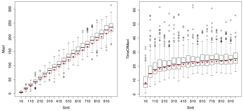
Figure 6.
Comparison of ODE (red dots) and Gillespie (200 replications) estimates of (left) and (right) for varying population sizes (between five and 1000 persons). The proximity of ODE red dots and boxplot median values highlights the remarkable matching between the two procedures, for parametervalues inferior to 500 individuals. Then, variance increases for Gillespie estimates, but impacting solely the indicator.
It appears from these results that there is no influence of the flight duration on the indicators. Therefore, it seems important to study whether or not the contagion process during flights had an influence on our indicators.
4.2.2. Impact of Contagion During Flights in MicMac
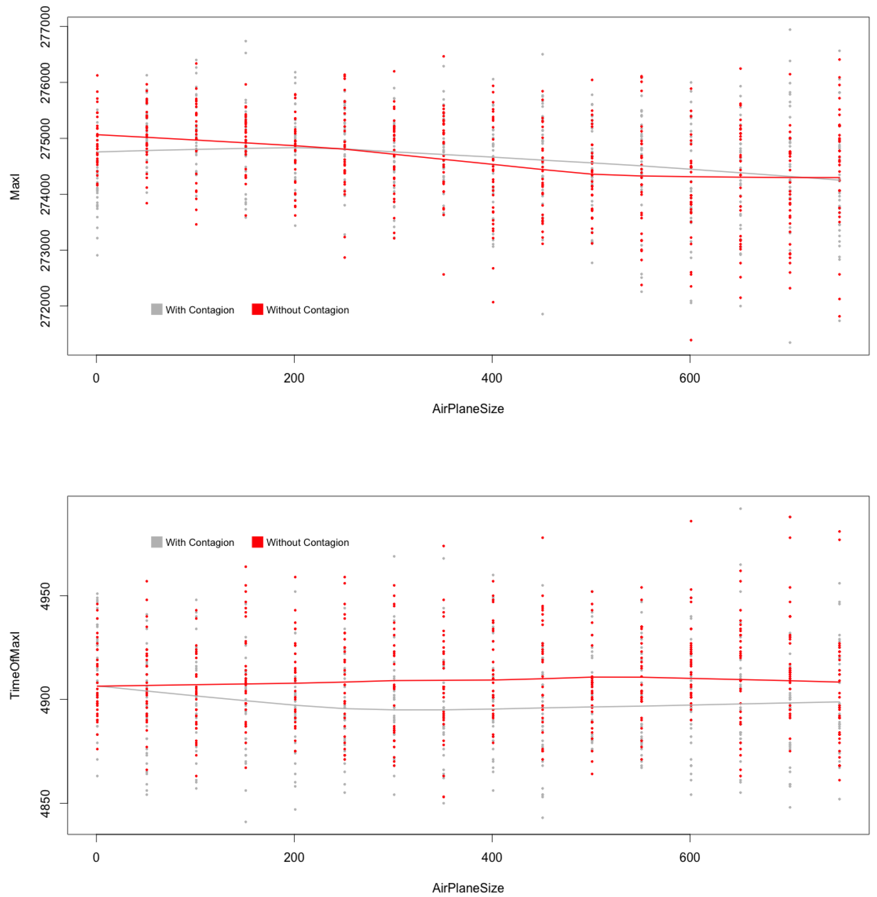
Finally, checking for specific impacts of contagion during flights leads to the following evidence: this process has no significant impact on the global epidemic dynamics; and clearly do not depend on the existence of such an internal dynamics during flights (see Figure 7). Indeed, the global dynamics is mainly due to dynamics occurring at city levels.
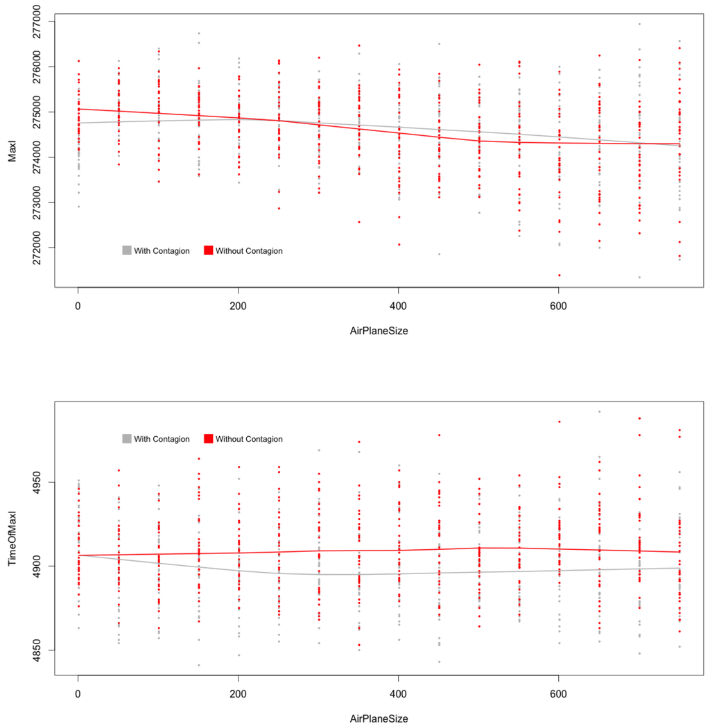
Figure 7.
(top) and (below) with and without contagion during flights, MicMac. Central lines are LoWeSS (locally weighted scatterplot smoothing) estimates, displaying the underlying central tendencies of the two populations being compared.
Figure 7.
(top) and (below) with and without contagion during flights, MicMac. Central lines are LoWeSS (locally weighted scatterplot smoothing) estimates, displaying the underlying central tendencies of the two populations being compared.
4.3. Impact of Network Topology in MetaPop and MicMac
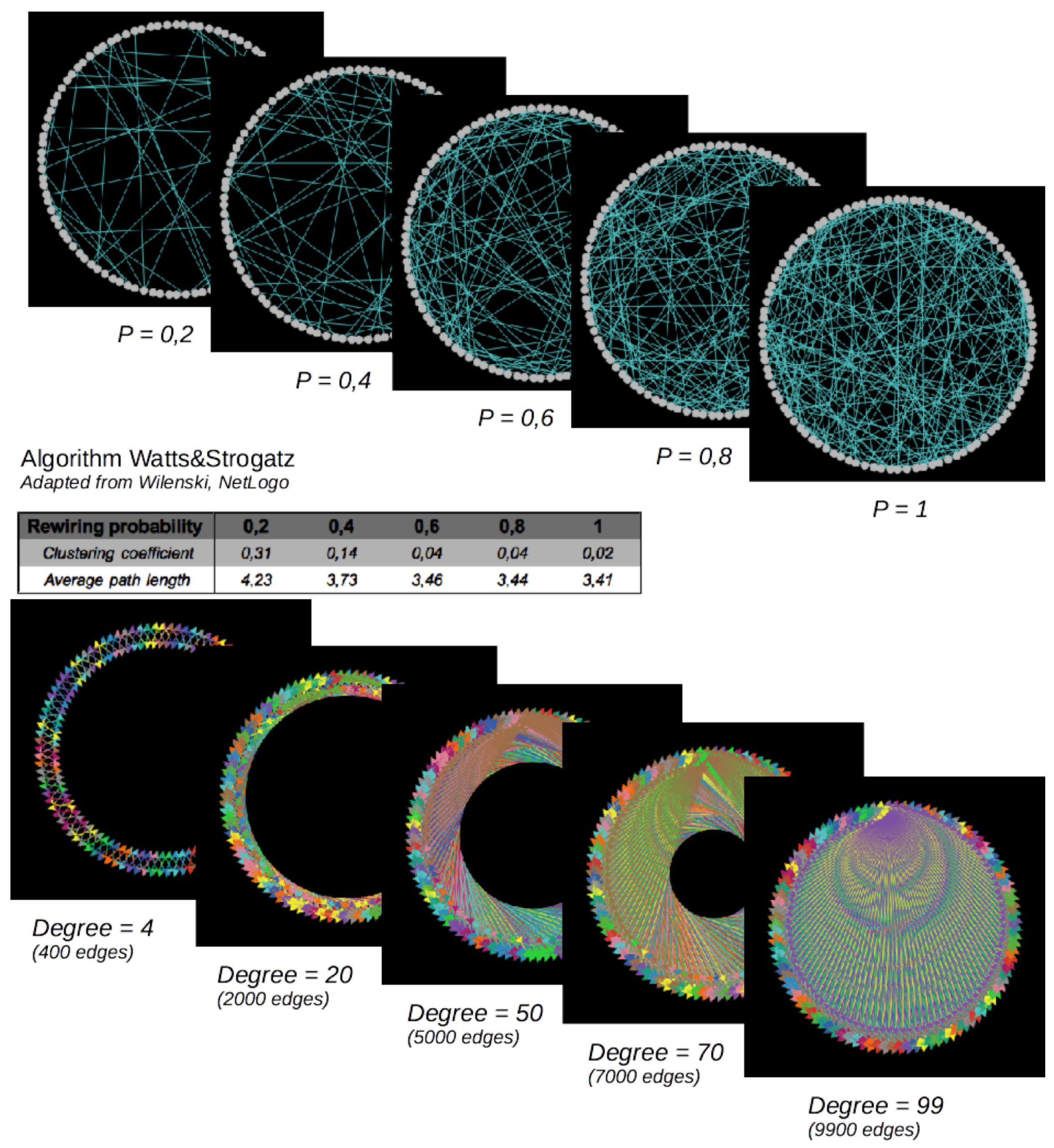
The network configuration (i.e., here, the way cities are connected) is known to impact the diffusion processes ([17,18]). In order to assess its role here, we define an experimental network composed of 100 nodes (cities). We compare more specifically a regular network, characterized by various node degrees (from four to 99 neighbors), and a small-word network, characterized by its rewiring probability. The latter is generated via the Watts and Strogatz algorithm [19]: we start with a regular network with a fixed degree of four neighbors for each node, and then, we rewire some of the nodes with a given probability. To evaluate the impact of various small-world networks, we consider rewiring probabilities from 0.2 to one (Figure 8).
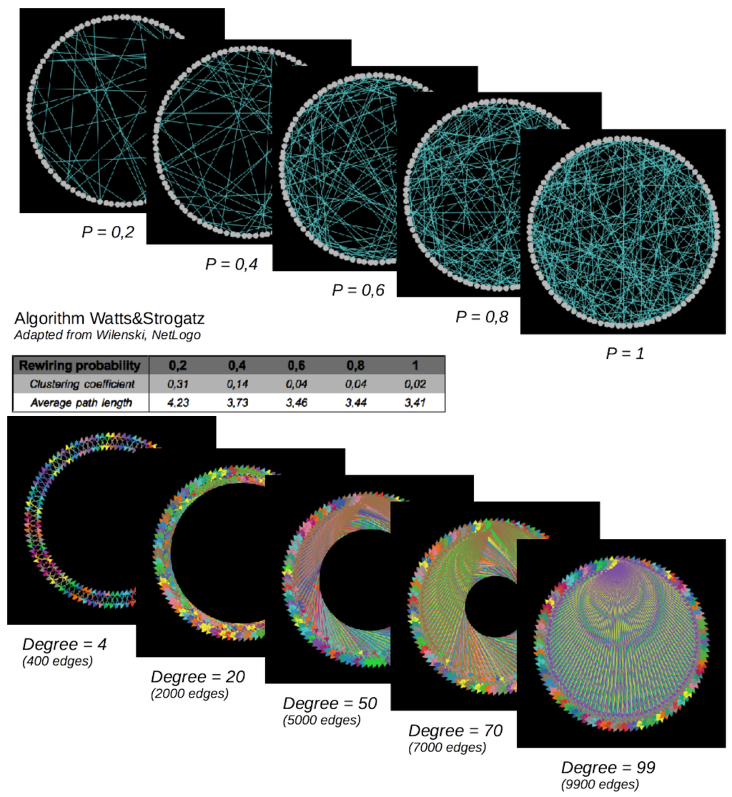
Figure 8.
Small-world (top) and regular networks (below). Number of nodes = 100. Small-world networks are random networks (in the sense that edges are defined randomly, based on the “rewiring probability”) characterized by short average path lengths and high clustering coefficients, varying with the “rewiring probability”, while the number of edges is held constant. Regular networks are characterized by an increasing number of edges here.
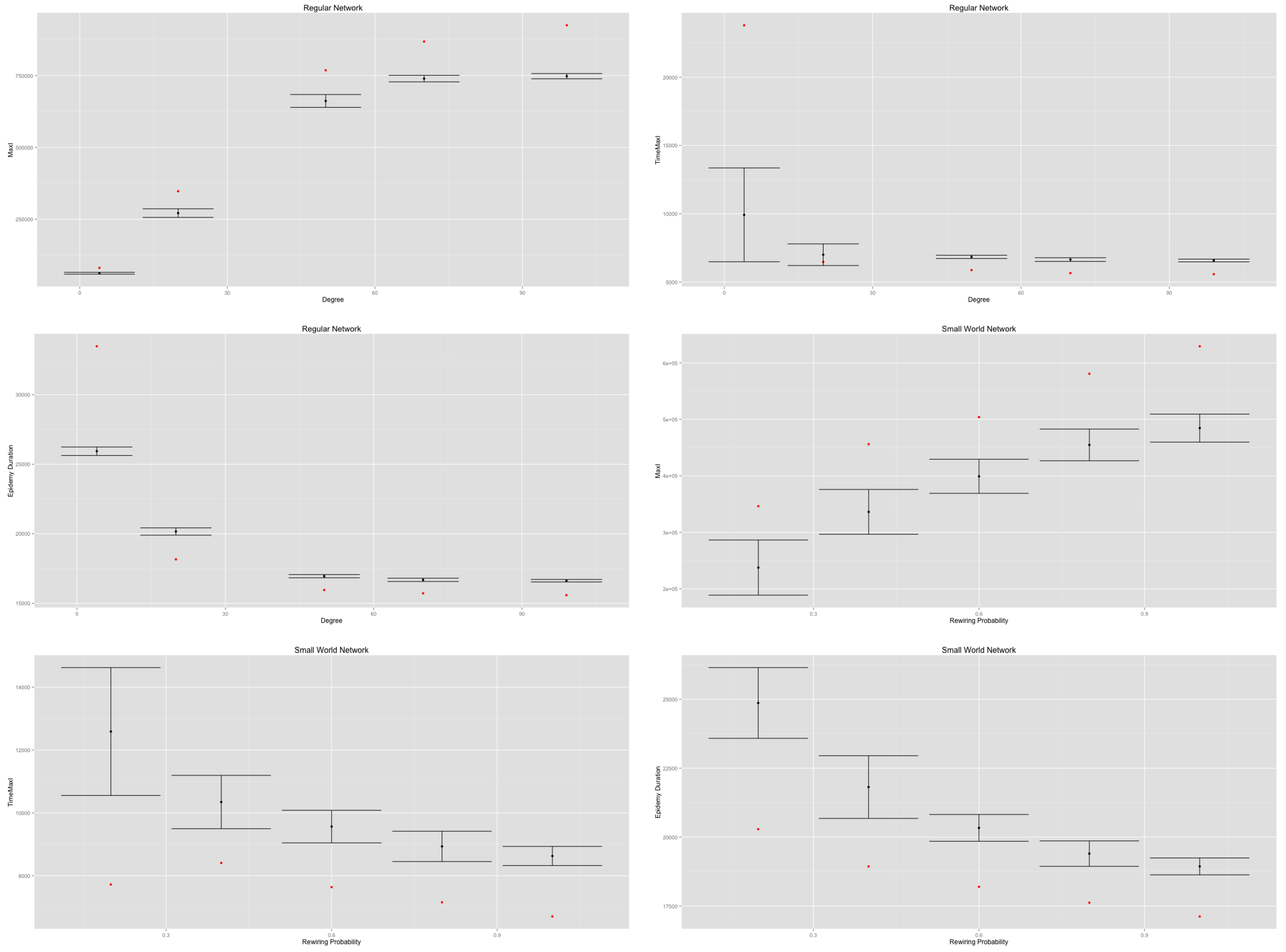
In both cases, an increasing density (regular networks) or an increasing rewiring probability (small-world networks) implies an increasing value of the value and a decreasing value of the and values (Figure 9).
Therefore, in both cases, increasing the density of networks decreases their diameter and their average path length, thus quickening the diffusion process. However, the MetaPop and MicMac models display different behaviors, as illustrated by the discrepancy between red dots (MetaPop) and error bars (MicMac). This is related to the continuous/discrete divergence that we raised at the end of Section 2: the continuous modeling approach accelerates the epidemic diffusion process in a significant way compared to the hybrid approach. Such divergence is likely to impact any containment or adaptive behavior that may be implemented and tested.
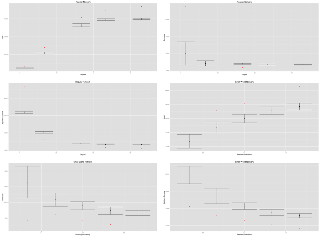
Figure 9.
Impact of regular network density and small-world network rewiring probability on on (top), in the (middle) and (below). Red dots correspond to the MetaPopmodel, while the error bars are drawn from 50 replications of the MicMac model. The discrepancy displayed between red dots (MetaPop) and error bars (MicMac) is related to the continuous vs. discrete anchorage of the two models.
5. Containment Strategy and Adaptive Behavior
We distinguish here a containment strategy and two adaptive behaviors, the three of them being implemented both in MetaPop and MicMac, as their microscopic foundations can be translated quite easily to macroscopic rules. The parameter values are given in Table 1.
The containment strategy is basically known as “quarantine”: cities are simply closed to traffic and cannot emit nor receive travelers. A city i is therefore quarantined if its rate of infected exceeds a threshold , i.e., if .
The first adaptive behavior is avoidance of at-risk destinations (called “avoidance”). A city i is avoided as a destination city if its infected rate exceeds a threshold , i.e., if . Contrary to quarantine, avoidance limits receptions, but not emissions, as an avoided city may still send travelers to other cities.
Finally, the second adaptive behavior is characterized by individual decisions not to travel while being infected, in order to avoid contributing to the spread of the on-going epidemic. We call this behavior “risk culture” and define it as follows:
- In MetaPop, the infected mobility rate in the city i is multiplied by a coefficient , varying between . If , city i will not emit infected people, and if , the mobility rate is unchanged.
- In MicMac, we define directly as a threshold, to which we compare the individual probability to travel for infected agents.
5.1. Quarantine
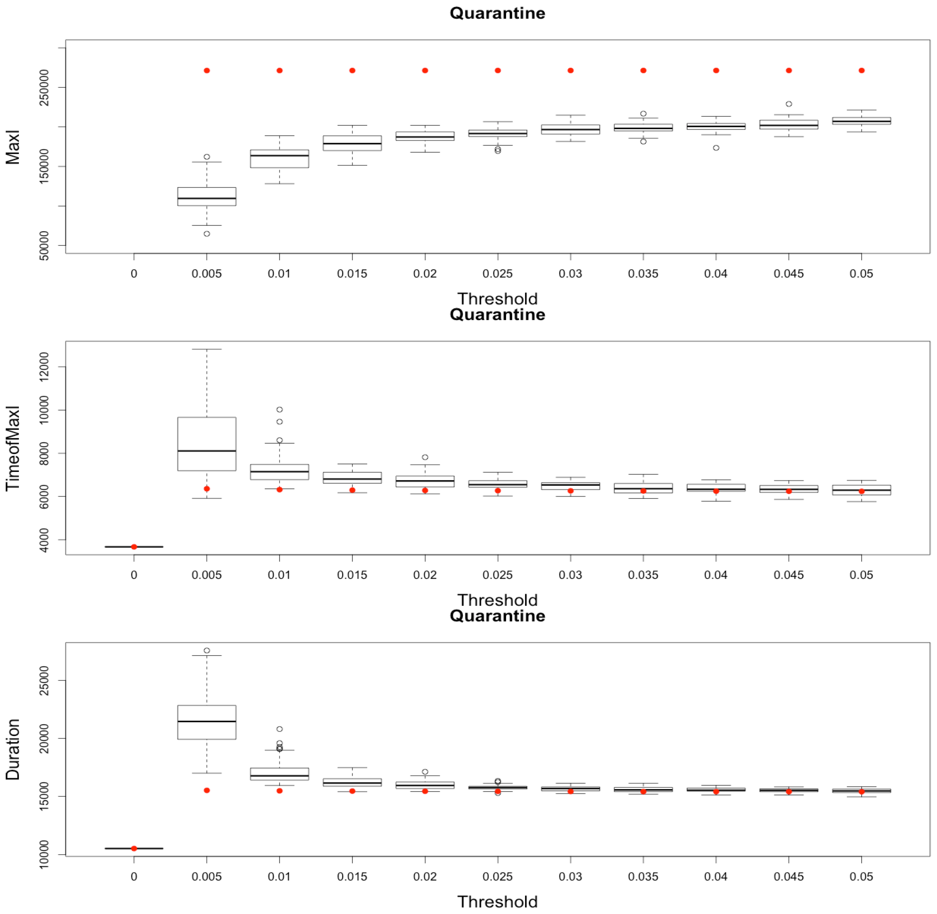
Comparing simulation outputs leads to a key idea: while the dynamics of the epidemic is largely driven by the SIR dynamics on nodes, composed of large static populations compared to small flying populations, the discretization and stochasticity implied by the agent formalism in the hybrid MicMac model provides a more progressive and realistic behavior of the epidemic (Figure 10).
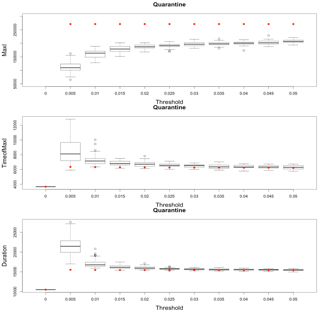
Figure 10.
Impact of various thresholds of quarantine setting-up on the epidemic, for the three indicators retained ( on (top), in the (middle) and (below)). Red dots correspond to MetaPop estimates and boxplots to MicMac estimates, for 50 replications. Threshold values correspond to the proportion of infected people in a node beyond which quarantine is setup (0.005 corresponds to five per-mille).
Indeed, in MetaPop, a unique time step is needed to infect every node from a single one in a complete network. Therefore, whatever the quarantine threshold, , is, always equals the sum of of all nodes, and the time to reach is equal to one time step.
In Micmac, diffusion occurs more gradually, mainly due to the discrete and stochastic mobility component: it takes more than one time step to infect all other nodes from a single infected person located on one node (Figure 11).
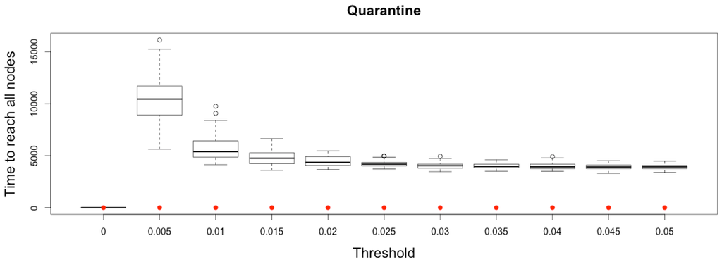
Figure 11.
Time to reach all nodes from one infected node () for various thresholds of quarantine setting-up. Red dots correspond to MetaPop estimates and boxplots to MicMac estimates, for 50 replications. Threshold values correspond to the proportion of infected people in a node beyond which quarantine is setup (0.005 corresponds to five per-mille).

This slight delay before infecting all the cities constitutes a short time window during which quarantine may prove its efficiency. This result outlines the importance of early detection of the disease and quarantine setting up.
5.2. Avoidance
While quarantine would impose a complete isolation of a city (whatever the practical difficulties of such an option may be), avoidance is merely an asymmetric process, limiting receptions, but not emissions, as an avoided city may still send travelers to other cities.
Therefore, the time needed to reach every other node from a seed one does not depend, in a complete network, on the avoidance threshold, as infected people may still travel to disease-free cities (see Figure 12).
However, simulation results are different from previous ones when it comes to epidemic indicators and underline, once again, different prediction capacities for the two models, as observed on Figure 13.
Indeed, as cities are infected as soon as the first iteration occurs for the MetaPop model (and with some delay for the MicMac model, but still in a uniform way), is reached more or less simultaneously for every node and converges towards its maximum theoretical value for the MetaPop model. However, still, as cities are closed in reception (activation of avoidance strategy) very early for low values of the avoidance threshold, their SIR dynamic starts with a very small value of I, and therefore, temporal indicators (time to reach and duration of epidemic) are increased for low threshold values. However, while MetaPop predicts a dramatic increase of epidemic durations for low values of the avoidance threshold, MicMac exhibits a more balanced behavior.

Figure 12.
Time to reach all nodes from one infected node () for various thresholds of avoidance setting-up. Red dots correspond to MetaPop estimates and boxplots to MicMac estimates, for 50 replications. Threshold values correspond to the proportion of infected people in a node beyond which avoidance is setup (0.005 corresponds to five per-mille).
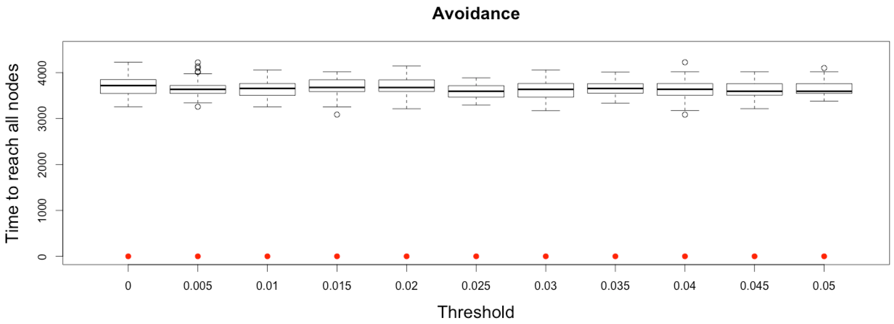
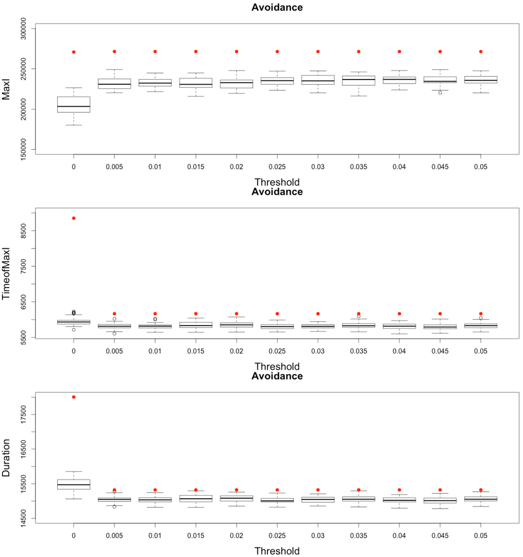
Figure 13.
Impact of various thresholds of avoidance setting-up on the epidemic, for the three indicators retained ( on (top), in the (middle) and (below)). Red dots correspond to MetaPop estimates and boxplots to MicMac estimates, for 50 replications. Threshold values correspond to the proportion of infected people in a node beyond which avoidance is setup (0.005 corresponds to five per-mille).
In conclusion, MetaPop predicts that early strategies of avoidance may not limit at all the epidemic burden and will moreover increase the global duration of the epidemic, while MicMac predicts an attenuation of epidemic severity and intensity.
5.3. Risk Culture
The third strategy we explore here corresponds to individual decisions not to travel while being infected, in order to avoid contributing to the spread of an on-going epidemic. This is done reducing the mobility rate of infected people by a coefficient lower than one.
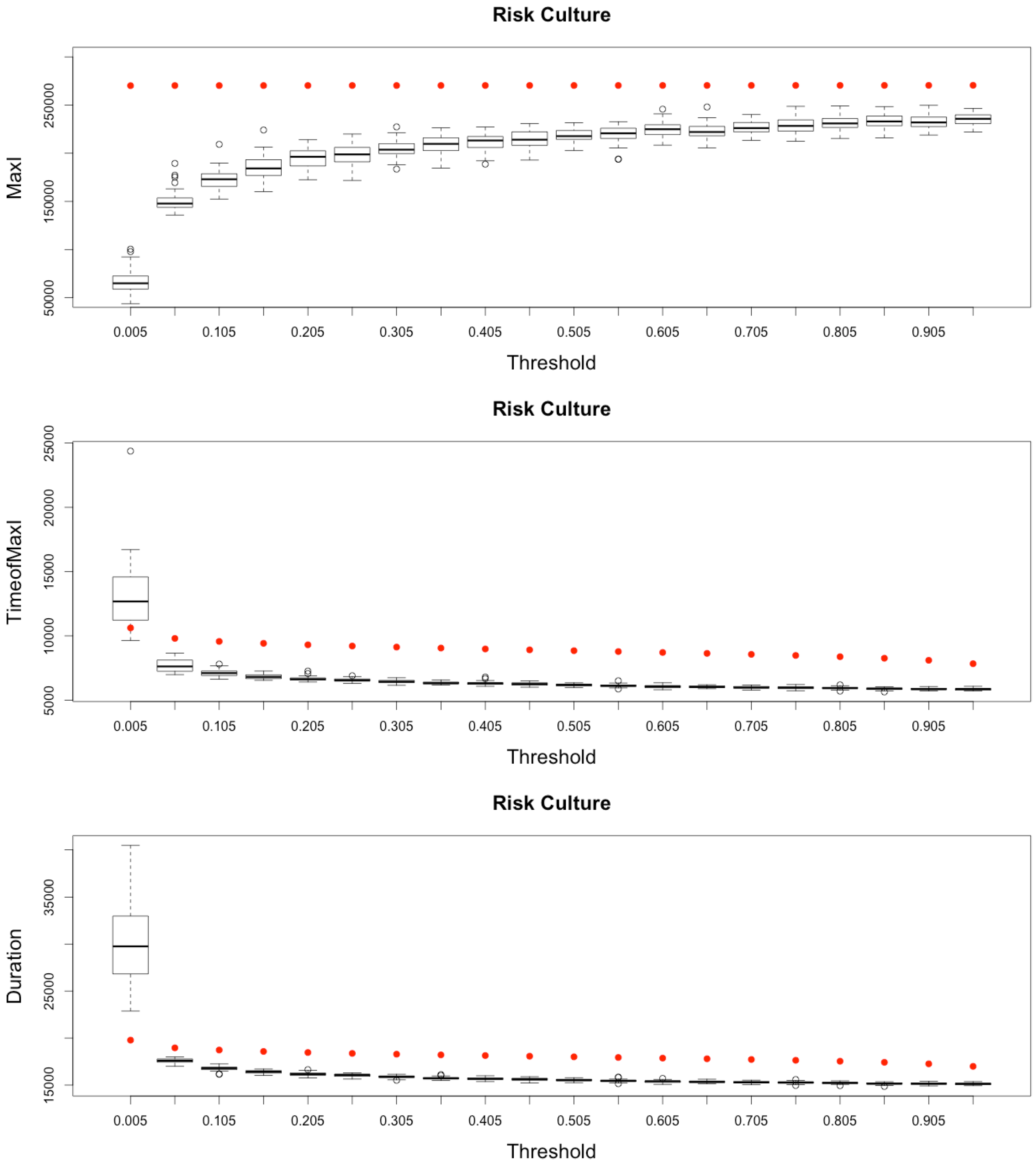
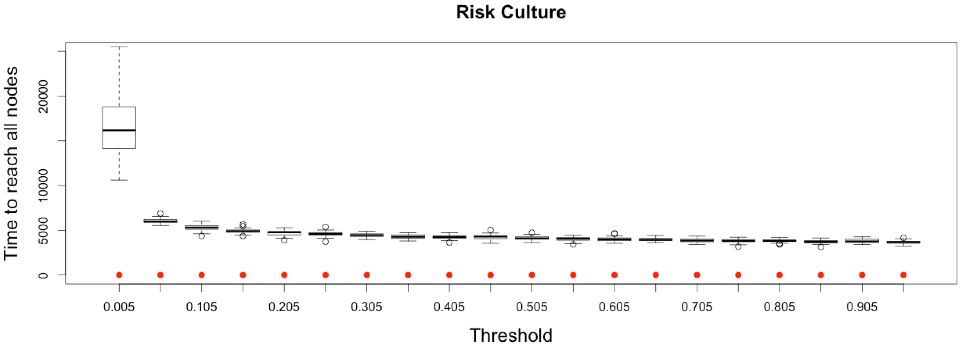
Here, again (see Figure 14), while MetaPop predicts no difference in the output when modifying the value of the reduction coefficient, MicMac predicts positive impacts of such a strategy, if applied early and in a drastic manner: epidemic intensity (as defined by ) may be clearly lowered while reasonably increasing the epidemic duration.
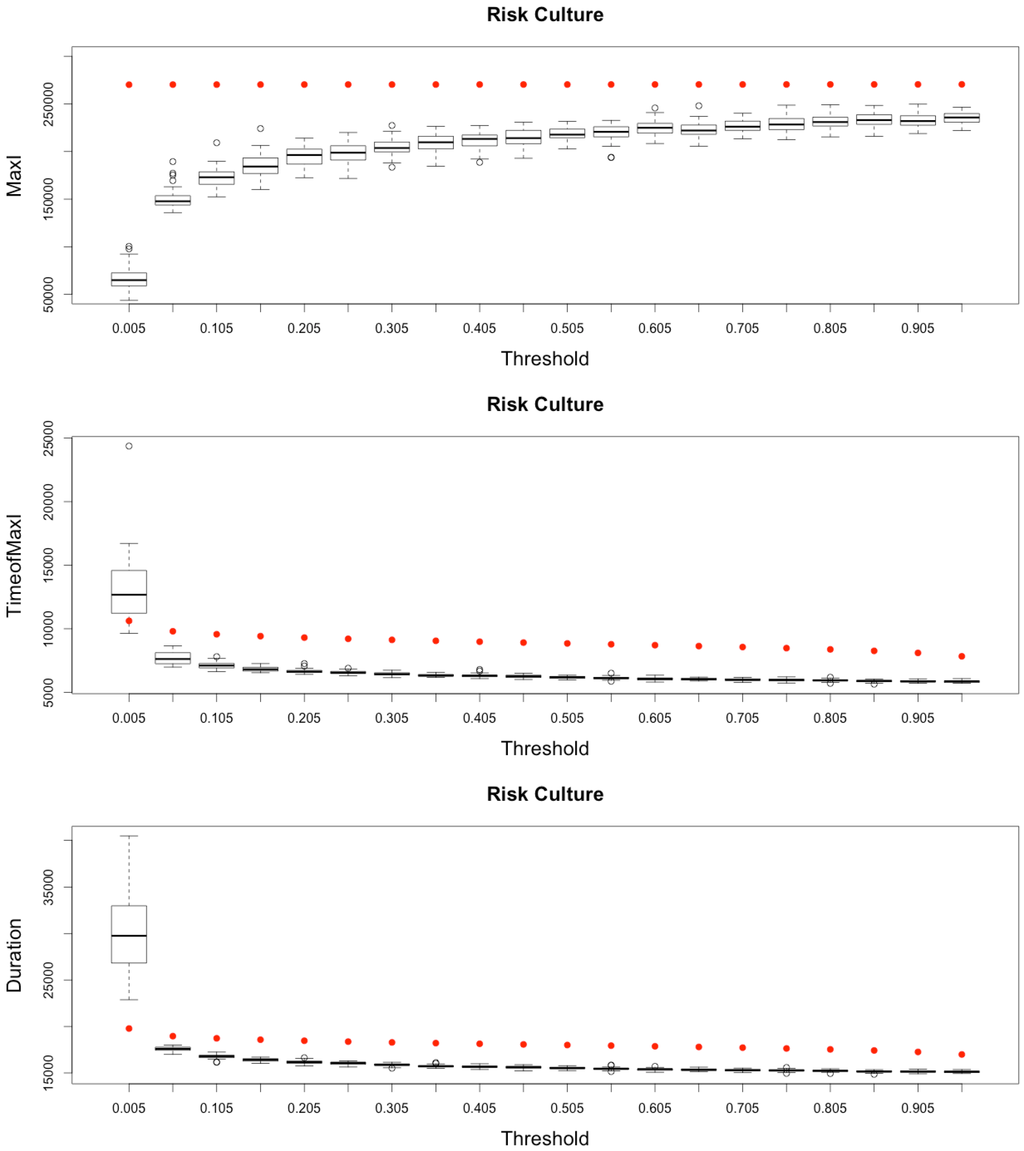
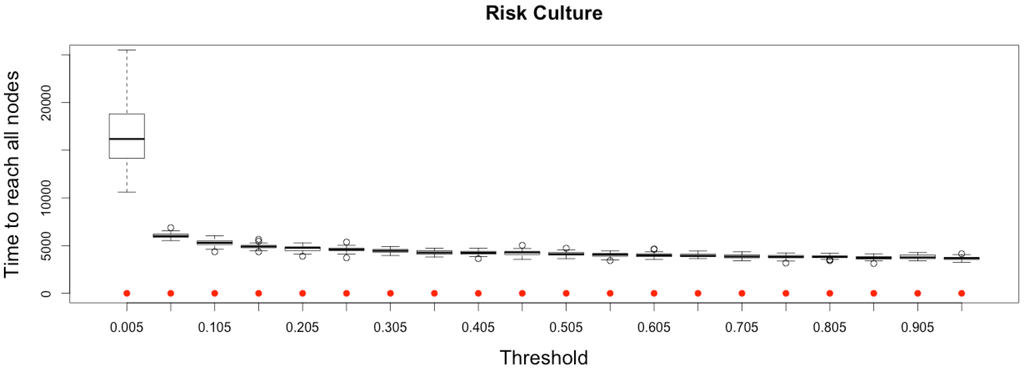
Figure 14.
Impact of risk culture on the epidemic, for the three indicators retained ( on (top), and in the (middle)) plus a fourth indicator of the time needed to reach all nodes from a single infected one (, (below)). Red dots correspond to MetaPop estimates and boxplots to MicMac estimates, for 50 replications. Threshold values correspond to reduction coefficients for the mobility rate in MetaPop and probabilities to travel when infected for MicMac. In both cases, a zero value of the threshold implies the absence of mobility for infected people.
6. Conclusion and Outlook
The diffusion of epidemics in space and time is a very active field of research, largely reinforced during the last twenty years, both by the various scientific dynamics in the field of complex networks, as well as the continuing emergence of new infectious diseases and their unprecedented rapid worldwide spread. In a highly connected and mobile world, modeling epidemic dynamics and their containment is still a hot societal and scientific topic. However, the spatial and temporal scales concerned today urge us to explore more hybrid models, combining the strengths and advantages of both macroscopic and microscopic paradigms. Building such hybrid models is far from easy, as it implies coupling processes occurring at different spatial and temporal scales, a frequent situation when working on city systems.
This paper is an attempt to progress in that direction in an as much as possible controlled manner. More specifically, we explored the possibilities of coupling models built at an aggregate scale (macroscopic), relying on a strong formalism and allowing theoretical results on large populations, with models at a more individual level (agents), allowing the integrating of mobility behavior in a more detailed way. Such coupling implies connecting these two approaches in space and time, and the adopted graph-based formalism provides a solid common basis for that perspective.
Starting from a full macroscopic model of coupled dynamical systems (MetaPop), we built a hybrid model (MicMac) in which both aggregate and individual behaviors are represented: an aggregate dynamics on nodes and an individual dynamics on edges. The aim of this work was to compare the MicMac hybrid model to the MetaPop aggregate one in order to underline the importance of being hybrid. If both models give the same results in the reference case (mean field approximation), the comparison clearly reveals a divergence when adding containment strategies and adaptive behaviors. Indeed, the results we obtain show how much richer the dynamics of the hybrid model is when it comes to taking into account these strategies.
These first results seem to make MicMac a relevant working basis for the exploration of epidemic dynamics at the level of a whole city system, including large-scale dynamics and individual behaviors, therefore allowing for more diversified and sophisticated adaptation strategies and control than those usually retained. Targeted upgrades of this model include the definition of routes, with intermediate stops, as well as the memory of nodes reached, allowing tracing back the spread of an epidemic. A second issue concerns the application of the model to real data, especially air traffic data. So far, we limited our investigations to theoretical networks, but the proposed model may be applied in a fairly straight manner to complex networks, characterized by heterogeneous contacts or degree correlations, for example [17,20]. We argue that the MicMac model, by its expressivity and flexibility, is able to tackle this challenge. A third issue is the automated calibration of containment and adaptive strategies, as well as the definition of a “cost” parameter, in order to explore optimal integrated strategies, allowing the fighting back of the epidemic while limiting its economic and social burden, two contradictory objectives. We do believe such integrating strategies, coupling processes and objectives in a more embedded way, will contribute to improving management of city systems, characterized by their ever-increasing complexity.
Acknowledgments
This work was founded by CNRS (Centre National de la Recherche Scientifique) via a PEPS (Projets Exploratoires Premier Soutien) HuMain (Humanités-Mathématiques-sciences de l’Information) in 2013 and 2014, and by the RNSC (Réseau national des systèmes complexes), via the interdisciplinary network MAPS (Modélisation multi-agents appliquée aux phènoménes spatialisés http://maps.hypotheses.org/).
Author Contributions
Every author equally contributed to the reported work.
Conflicts of Interest
The authors declare no conflict of interest.
References
- Hanski, I.; Gilpin, M.E. MetaPopulation Biology: Ecology, Genetics, and Evolution; Academic Press: Waltham, MA, USA, 1997. [Google Scholar]
- Levins, R. Some demographic and genetic consequences of environmental heterogeneity for biological control. Bull. Entomol. Soc. Am. 1969, 15, 237–240. [Google Scholar] [CrossRef]
- Arino, J.; van den Driessche, P. A multi-city epidemic model. Math. Popul. Stud. 2003, 10, 175–193. [Google Scholar] [CrossRef]
- Colizza, V.; Vespignani, A. Epidemic in MetaPopulation modeling systems with heterogeneous coupling pattern: Theory and simulations. J. Theor. Biol. 2008, 251, 450–467. [Google Scholar] [CrossRef] [PubMed]
- Meloni, S.; Perra, N.; Arenas, A.; Gomez, S.; Moreno, Y.; Vespignani, A. Modeling human mobility responses to the wide-scale spreading of infectious diseases. Sci. Rep. 2011, 1, 1–7. [Google Scholar] [CrossRef] [PubMed]
- Durrett, R.; Levin, S. The importance of being discrete (and spatial). Theor. Popul. Biol. 1994, 46, 363–394. [Google Scholar] [CrossRef]
- Fahse, L.; Wissel, C.; Grimm, V. Reconciling classical and IB Approaches in theoretical population ecology: A protocol for extracting population parameters from IBM. Am. Nat. 1998, 152, 838–852. [Google Scholar] [CrossRef] [PubMed]
- Frontier, S.; Pichod-Viale, D. Ecosystèmes, Structure, Fonctionnement, Evolution; Masson: Paris, France, 1990. [Google Scholar]
- Ajelli, M.; GonCalves, B.; Balcan, D.; Colizza, V.; Hu, H.; Ramasco, J.J.; Merler, S.; Vespignani, A. Comparing wide-scale computational modeling Approaches to epidemic: Agent-based versus structured MetaPopulation models. BMC Infect. Dis. 2010, 10, 350–352. [Google Scholar] [CrossRef] [PubMed]
- Nguyen, N.D. Coupling Equation-based and Individual-based Models in the Study of Complex Systems—A Case Study in Theoretical Population Ecology. Ph.D. Thesis, Pierre and Marie Curie University, Paris, France, 2010. [Google Scholar]
- Kermack, W.O.; McKendrick, A.G. Contributions to the mathematical theory of epidemics. J. Hyg. 1939, 39, 271–288. [Google Scholar] [CrossRef] [PubMed]
- Brauer, F.; van den Driessche, P.; Wu, J. Mathematical Epidemiology; Springer: Berlin, Germany, 2008. [Google Scholar]
- Banos, A.; Corson, N.; Gaudou, B.; Laperrière, V.; Rey Coyrehourcq, S. Coupling micro and macro dynamics models on networks: Application to disease spread. In LNCS Lecture Notes in Computer Science; Springer: Berlin, Germany, 2015. [Google Scholar]
- Bureau of transportation Statistics. Available online: http://www.rita.dot.gov/bts/data_and_statistics/index.html (accessed on 12 December 2014).
- Gillespie, D.T. A general method for numerically simulating the stochastic time evolution of coupled chemical reactions. J. Comput. Phys. 1976, 22, 403–434. [Google Scholar] [CrossRef]
- Gillespie, D.T. Exact stochastic simulation of coupled chemical reactions. J. Phys. Chem. 1977, 81, 2340–2361. [Google Scholar] [CrossRef]
- Keeling, M.J. The effects of local spatial structure on epidemiological invasions. Proc. R. Soc. Lond. B 1999, 266, 859–867. [Google Scholar] [CrossRef] [PubMed]
- Pastor-Satorras, R.; Castellano, C.; van Mieghem, P.; Vespignani, A. Epidemic processes in complex networks. Eprint Arxiv 2014, 363, 120–131. [Google Scholar] [CrossRef]
- Watts, D.J.; Strogatz, S.H. Collective dynamics of “small-world” networks. Nature 1998, 393, 440–442. [Google Scholar] [CrossRef] [PubMed]
- Wang, Y.; Cao, J.; Alofi, A.; AL-Mazrooei, A.; Elaiw, A. Revisiting node-based {SIR} models in complex networks with degree correlations. Phys. A 2015, 437, 75–88. [Google Scholar] [CrossRef]
© 2015 by the authors; licensee MDPI, Basel, Switzerland. This article is an open access article distributed under the terms and conditions of the Creative Commons Attribution license (http://creativecommons.org/licenses/by/4.0/).
