Abstract
In comparison to their performance with normative standards or even simple heuristics, humans do not perform well in complex decision-making. The application of systems thinking to help people to understand and handle interdependent and complex systems is proposed as a means of improving this poor performance. The aim of this study is to investigate the effect of a generic systems thinking method, i.e., a structured method, on performance. A laboratory experiment was conducted using a dynamic and complex simulation task. The results demonstrated that subjects provided with a structured method achieved a higher performance. In addition, mental model accuracy had a significant effect on performance, as already shown by several previous studies. The results of our study provide a way of teaching subjects how to improve their performance when coping with complex systems in general. This has implications for education in the fields of complex systems and system dynamics.
1. Introduction
The question of how to improve the performance of people who need to control complex systems has become increasingly important. Several methods for dealing with complexity are discussed in the literature, such as in in Größler, Maier, and Milling [1], Capelo and Dias [2], Ritchie-Dunham [3], Rouwette, Größler and Vennix [4], Sengupta and Abdel-Hamid [5], Richmond [6], Sterman [7], Sweeney and Sterman [8]. However, less attention has been paid to so-called “heuristic competence” [9]. Not a well-defined term, it indicates the general ability of a subject to perform well in complex systems. Our study tries to shed further light on the ability of “heuristic competence”.
Many experimental studies show that subjects, in contrast to their performance with normative standards or simple heuristics, do not perform well in complex decision-making (e.g., [10,11,12,13]). Different characteristics of a system lead to this poor performance. Misperception of feedback relations is one of the more important causes of poor performance [10,11,12]. In addition to feedback relations, the concept of accumulation is also a reason [13,14]. Two insufficiencies may also result in poor performance: first, mental models of the causal structure of systems are highly simplified compared to reality. Mental models are abridged, analogous representations of an external system inside a person’s mind [15,16]. The second insufficiency is a person’s inability to infer the dynamic behavior of such causal structures [7].
The literature discusses several ways of enhancing the decision-making of subjects in complex systems. Providing structural information about the underlying system in order to increase transparency seems to have a positive effect on performance [1,2,3]. Knowledge of cause-and-effect relationships supports learning and the development of mental models which are more similar to a real system. These more accurate mental models lead to a higher performance [17,18].
In addition to a greater transparency to facilitate learning, different kinds of decision information and their presentation have also been investigated. Outcome feedback is present in all studies that use simulators, because subjects need to be provided with the results of their previous decisions [4]. Subjects’ performance did improve when they were provided with cognitive feedback or feedforward in comparison to outcome feedback alone [5,19,20].
The last approach for enhancing complex decision-making that should be mentioned, is the application of systems thinking. Systems thinking is a conceptual framework for handling and understanding interdependent and complex systems [6,7]. It consists of knowledge, tools, and techniques developed for analyzing and handling systems and their inherent complexity [21,22]. Overcoming barriers to learning in such systems is a critical element and needs several requirements and thinking skills. Generally, even highly educated subjects exhibit persistent and systematic errors in the application of systems thinking and its basic concepts.
The literature provides a large number of structures and schemes for systems thinking. To name but a few authors: Gharajedaghi [23] defined four foundations of systems methodology (holistic thinking, operational thinking, systems theories, interactive design); Senge [21] stated five disciplines of the learning organization (systems thinking, personal mastery, mental models, shared vision, team learning); based on Senge, Frank [24] developed thirty laws of engineering systems thinking, Richmond [6] listed seven critical skills for systems thinking (dynamic, closed-loop, generic, structural, operational, continuum, scientific), and Valerdi and Rouse [25] presented seven competencies [26] for systems thinking.
Despite this previous work and the widespread use of systems thinking (e.g., [27,28]), there has been a more recent call for empirical work to analyze the relationship between systems thinking and mental models or decision-making processes [29]. The current study addresses this empirical research gap by examining a specific structured method of thinking as an iterative approach to learning about and dealing with a complex task.
In an exploratory study, Maani and Maharaj [30] examine the link between systems thinking and complex decision-making. A total of ten subjects participated in an interactive, computer-based simulation while being asked to verbalize their thoughts. The protocols were analyzed to see whether more systems thinking, or certain dimensions of it, might have an impact on the performance in a complex task. In addition to finding Richmond’s [6] dimensions of systems thinking to be relevant, they found a specific pattern of behavior which differentiated high and low performers. This pattern, which Maani and Maharaj [30] called the “CPA cycle”, consists of a series of three phases: Conception, Planning, Action.
Our study investigates the relationship between a structured method, i.e., the CPA cycle of Maani and Maharaj [30], and mental model accuracy and performance. A laboratory experiment was duly designed and conducted. A complex and dynamic simulation task was used to investigate the proposed link between the dependent and independent variables. The results show a positive impact of a structured method on performance, but no impact on mental model accuracy. Mental model accuracy itself shows a high effect on performance. The last finding is comparable to earlier studies.
The remainder of this article is organized as follows. Section 2 provides an overview of the theory and states the proposed hypotheses. Section 3 describes the course of the experiment, measurement variables, and statistical methods used for analyzing the data. Results are illustrated in Section 4. Section 5 concludes with a discussion of the findings, limitations, and implications, together with future research directions.
2. Theory and Hypotheses
The findings of Maani and Maharaj [30] suggest that the use of a structured method may enhance subjects’ performance in a complex task. A structured method is defined as a thinking pattern that structures the process of collecting information, developing appropriate strategies, and implementing these into actions. A structured method, the authors found, has three distinct phases:
- Conception
- Planning
- Action
In the first step—the conception phase—subjects try to gain an understanding of the structure of a problem. Transferred to the task used in the experiment of managing a start-up company, this would, for example, mean identifying a backlog of orders. Particularly in this phase can systems thinking be used. Following on from the conception phase is the planning phase. One or more strategies for handling the problem are developed. These are, ideally, based on the understanding gained from the previous phase. With regard to this example, production capacity could be increased or the price could be raised in order to reduce the number of new orders and to catch up with the existing orders. Eventually, a decision for one strategy is made, and this strategy is implemented through specific actions: The price is raised by a specific amount that relates to the size of the backlog. It is important to note that in order to be effective, the CPA cycle needs to be iterative. The action phase of one cycle should lead to the conception phase of a new cycle. Especially in a complex and opaque task, an understanding can only be gained progressively.
One limitation of their study is the small sample size of ten participants, which is a result of the applied research method. Due to the high density of data and the labor-intensive analysis of verbal protocols, the sample size of verbal protocol analysis is commonly between two and 20 persons [31], leading to an exploratory orientation.
Our research focuses on how the CPA cycle enhances information usage, strategic planning, and implementation, aiming to achieve an increased understanding of the underlying structure of the task and enhanced performance. The expected relationships and hypotheses are illustrated by the research model in Figure 1.
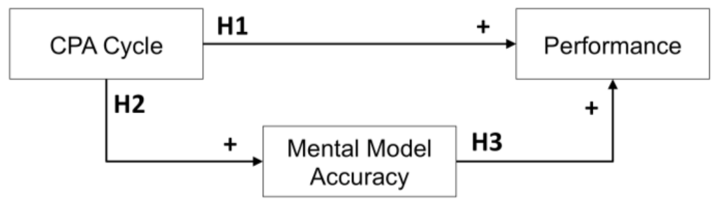
Figure 1.
Proposed research model.
Hypothesis 1: The use of the CPA cycle positively influences performance in the complex task.
Subjects who follow the CPA cycle should be able to use given information in a more effective way, especially with the aim of developing strategies and translating them into action. The information processing capabilities of the subjects should be enhanced [32]. Thus, the CPA cycle is an information-driven method with a focus on the implementation of strategies. As a result, subjects should tend to learn and act more effectively. Ultimately, this leads to higher performance in the experimental task.
Hypothesis 2: Application of the CPA cycle results in a more accurate mental model of the underlying system in the complex task.
Enhanced learning on account of the CPA cycle helps subjects to acquire a better understanding of the underlying system and a deeper assessment of the consequences of their decisions. Feedback on the system leads to a re-evaluation of the mental model of the system. Assumed relationships between variables may be altered and new ones may be added, resulting in an improved understanding. This also enhances subjects’ ability to build more accurate mental models. The changed mental model induces different strategies and decisions affecting future behavior [2,7]. This process is iterative.
Hypothesis 3: Higher mental model accuracy is associated with higher performance in the complex task.
Subjects with more accurate beliefs about the causal relationships in a system are supposed to achieve a superior performance. These subjects are able to assess the effects that may result from different actions in a given situation. In general, they are more likely to identify and follow effective strategies to achieve success. This positive relationship between mental model accuracy and performance outcome is well established in the literature [2,3,17,18]. Maani and Cavana [33] developed an analogy of an iceberg for a conceptual model which can relate behavior to mental models. The behavior or the decisions made are visible above the waterline. The mental model itself, which reflects beliefs, assumptions, or values, is at the deepest level. These two levels are linked by two further levels: first, the systemic structure shows the relationships of the different components. Second, the patterns of a larger set of behaviors are deduced from past behaviors or outcomes [28].
Hypothesis 4: The relationship between the use of the CPA cycle and the performance in the complex task is mediated by mental model accuracy.
The proposed research model in Figure 1 specifies a mediation model, where Hypothesis 1 indicates a direct effect, while Hypotheses 2 and 3 together constitute an indirect effect of the CPA cycle on performance in the complex task. As a result, Hypothesis 4 is derived. The use of the CPA cycle results in a more accurate mental model of the underlying system, i.e., learning, which then leads to a higher performance in the complex task.
3. Methods
To test the stated hypotheses, we conducted an experiment. It incorporated two treatments: a control treatment and a CPA treatment. In the latter, subjects were taught how to use the CPA cycle. An interactive computer simulation was used as a complex task. This simulation represented a fictitious start-up company. Subjects controlled three decision variables: market price, investment in production capacity, and marketing spending. Performance was measured through cumulative profit.
3.1. Participants and Design
In total, 58 students from a major German university participated in the experiment. Four subjects had to be excluded. One subject broke off participation during the course of the experiment, one subject failed to understand the task because of insufficient language skills, and two subjects showed a huge deviation in their performance in the third trial of the task from their first two trials. This resulted in a final sample size of 54 subjects.
Of the remaining students, 34 were male and 20 were female. The average age was 23.6 years (SD = 3.4). A one-factorial between-subjects design was used for the experiment. All subjects were randomly assigned to one of the two treatments. 30 subjects participated in the control group, while 24 formed the CPA group. The average payment for participating was 14.21 € (about $15.50) with a minimum of 12 € and a maximum of 18 €.
Table 1 summarizes the demographics of the participants. The participants were mostly male students, about half of them studying engineering or industrial engineering, followed by business/management science. The rest of them are distributed across natural science, such as biology or physics, and ‘other’. The latter in this case comprised medical or political science, geography, and linguistics.
A comparison of the two groups did not reveal any significant differences. The t-test for comparing the age of both groups is not significant (t (51) = 1.46, p > 0.15). To test for independence between the categorical data of gender and group and field of study and group, respectively, Fisher’s exact test was used. Fisher’s exact test allows expected frequencies to be less than four and the matrices to be larger than 2 × 2, as is the case here [34]. The null hypothesis that ‘gender’ and group are stochastically independent cannot be rejected (p > 0.78, Fisher’s exact test). The same holds for “field of study” and group (p > 0.36, Fisher’s exact test).

Table 1.
Subject demographics.
| Variables | Control Group | CPA Group | |
|---|---|---|---|
| Age | M | 24.17 | 22.88 |
| SD | 3.88 | 2.59 | |
| N | 30 | 24 | |
| Gender | Male | 18 | 16 |
| Female | 12 | 8 | |
| Field of study a | Engineering | 12 | 5 |
| Industrial Engineering b | 5 | 9 | |
| Business/Management | 7 | 5 | |
| Science | 3 | 3 | |
| Other c | 3 | 1 | |
a One subject did not answer this question; b The degree program “Industrial Engineering” is comprised of lectures on both business and engineering. This degree program is particularly popular at the German university where the study took place; c “Other” includes medical science, political science, geography, and linguistics. There was only one student from each of these disciplines.
3.2. Simulation Overview
The participants run a simulation of a start-up company by making decisions every three months over a period of four years. This makes for a total of 16 decision points. The start-up company introduces a new product to the market. Due to the novelty of the product, it is assumed that the company is a monopolist, so there is no competition during the whole time horizon of the simulation. The decision maker has to decide about production capacity, selling price, and marketing budget per quarter. Figure 2 presents a simplified representation of the underlying causal relationships of the simulation, associated with different areas, such as production, demand, and accounting. This shows how the variables are interrelated.
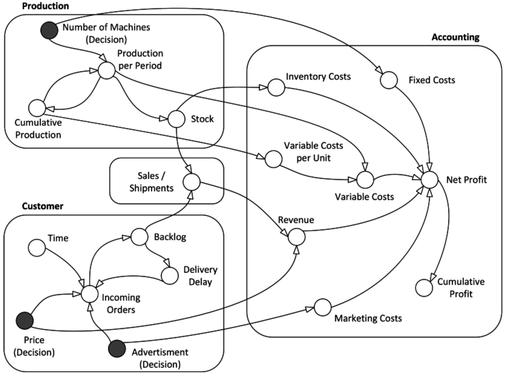
Figure 2.
Causal relationships of the simulation (simplified).
Participants analyze the status of the company and make decisions based on the obtained information. The selling price and the marketing budget can be set within a given range. The price elasticity of demand is inelastic in the high and low price areas, while it is near to unity in the middle of the spectrum. The effect of the marketing effort is diminishing, and the effect also depends on the price. To increase the capacity, new machines could be acquired, which would be ready to use with a one-quarter delay. The company follows a make-to-stock strategy. Storage capacity is assumed to be unlimited. If products are stocked, incoming orders are fulfilled immediately, otherwise the orders enter the backlog and are fulfilled when more products become available. A high backlog has a negative effect on incoming orders because of the low delivery capacity of the company. On the other hand, a high stock leads to inventory costs. The game interface can be seen in Figure 3. It was translated from the German.
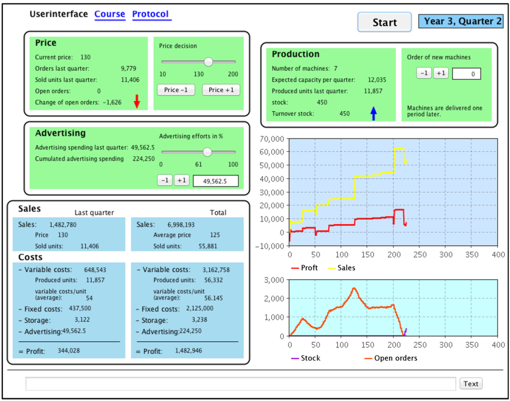
Figure 3.
Simulator interface for controlling the task (translated from the German).
Profit is calculated as revenues minus expenses. Revenues are determined by the number of sold products in a quarter multiplied by the price of this time period. The expenses are the sum of the fixed costs, the variable costs, and the marketing expenses. Fixed costs are calculated proportionally to the number of machines. Variable costs are proportional to the production of the period, taking into account the learning curve effect. Marketing expenditure is defined by the subject within a range of zero and a maximum given marketing budget. Regardless of any losses, the company cannot go bankrupt.
During the simulation, participants were able to access outcome feedback in the form of financial and non-financial information about the current state of the company. Extensive information about former periods was available during each run of the simulation in the form of graphical representations. A number of variables were offered for selection, such as profit, sales, orders, or production in order to display graphically the entire history up to the current period or a specified quarter. The interface for obtaining information is presented in Figure 4.
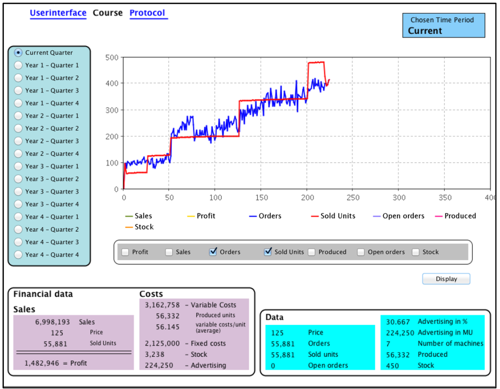
Figure 4.
Simulator interface for obtaining information (translated from the German).
3.3. Procedure
Subjects were randomly assigned to one of the two treatments. First, both treatment groups participated in an interactive, computer-based learning program. In the CPA treatment, the learning program consisted of information about the different phases of the cycle, as given by Maani and Maharaj [30]. Following the explanation of each step of the CPA cycle, a small case study was presented. This case study was solved by explicitly referring to the CPA cycle. Several multiple-choice questions and a test at the end of the program facilitated the learning success. The control group took part in a learning program with a similar structure, but which included nothing that was relevant to the task that followed. The control group undertook this program to avoid any potential motivational effects given by an upstream task. The learning program represents a transfer of explicit knowledge [35]. Explicit knowledge can be codified and is context-independent [36].
Subsequent to the learning program, all subjects completed three runs of the simulation. The simulation had the same underlying structure and initial conditions for both treatments. Subjects were given detailed instructions on the simulation. In order to become familiar with the simulation and the interface, the first two runs were defined as a learning phase. During the simulation participants could obtain outcome feedback in the form of financial and non-financial information (see Figure 3 and Figure 4).
Following on from this learning phase, subjects were asked to complete a questionnaire on the underlying structure of the simulation. This was done in order to assess the mental model of the underlying structure by each participant. The employed elicitation method constitutes a combination of Markiczy and Goldberg [37] and the pairwise comparisons mapping of Hodgkinson, Maule, and Bown [38]. A preliminary test revealed that the participants had considerable problems using the cognitive mapping approach of Markiczy and Goldberg [37] due to the unfamiliarity of the task. This led to the development of a questionnaire (the pilot test was conducted to assess the procedure and comprehensibility of the experiment. Additionally, changes in the elicitation method of mental models, it led to minor changes in provided documents).
The questionnaire consisted of 25 questions on bivariate causal relationships between existing and non-existing variables in the underlying system. The set of questions was the same for both treatments. For each question, the subjects had to decide whether there was a positive, a negative, or no relationship at all between the two given variables.
The number of correct answers as the percentage of all items in the questionnaire was used to assess mental model accuracy. The score ranged from 0% to 100%, with 100% meaning that all questions had been answered correctly. Participants were provided with a monetary incentive depending on their performance in this task.
After completion of the questionnaire on the mental model, all subjects performed a final run of the simulation. They were prompted to try to achieve the highest possible cumulative profit. The final profit measure served as a performance indicator. In particular, a high performance was monetarily incentivized to motivate subjects and to strengthen the reliability of the measure.
The experiment ended with a questionnaire on demographics and general questions about the learning program, the simulation, and the mental model elicitation. After this, participants were paid individually and left the laboratory.
3.4. Measures
Performance was measured by cumulated profit of the third and final run of the simulation. As previous runs were treated as a learning phase, they had no influence on subjects’ performance. The performance of the final run was monetarily incentivized.
Subsequent to the learning phase, participants’ understanding of the underlying structure of the simulation, i.e., the mental model, was captured. All subjects answered 25 questions on the underlying structure of the simulation. Appendix A provides the instructions along with examples of the questions. All questions had to be answered. The option “No Answer” was offered in case subjects were unsure about their answer. They were asked to select this option rather than randomly guessing. This approach was used in order to increase the reliability of the response.
The questions were the same for both treatment groups. The variable “mental model accuracy” was calculated as a percentage of correct answers, resulting in a range from 0% to 100%, with 0% meaning no understanding at all and 100% meaning a full understanding.
Through examination of the structure and the dynamics and behavior of the simulation, a subset of causal relationships was identified. These serve as key correcting variables. This subset consists of six out of 25 bivariate relationships and forms the deep structure of the simulation. There are two different groups in the subset: The first group consists of cost relationships; the second one of control factors. In the system at hand, knowledge of the cost relationships should enable subjects to identify important factors which significantly influence the objective criterion. The control factors, on the other hand, put subjects in a position where they can influence the system according to the cost relationships and finally enable them to achieve a high cumulative profit. The calculation and range are similar to mental model accuracy. The deep structure variable consists of six items of the questionnaire addressing participants’ understanding of the structure, while the remaining 19 items form the non-deep structure.
In addition to the stated variables, the following variables were recorded: the time it took to perform each of the three runs of the simulation; the time necessary to complete the respective learning program; the time for answering the 25 questions on mental model accuracy; a participant’s age and experience, measured in terms of work experience and the number of economics lectures attended. Economics lectures were included, because these might have an effect on the behavior of participants in an economics task like the one at hand. It also might be relevant to subjects’ responses to the test of their understanding of the mental model.
3.5. Data Analysis
The Shapiro-Wilk test was used to test for normality of the dependent variable. The performance measure is significantly non-normal distributed (W = 0.81, p < 0.001), given the high negative skewness. Due to the skewed distribution of the dependent variable, generalized linear models were estimated using a Poisson link function. It may be noted that in a Poisson regression, the dependent variable is the log of the conditional mean. A regression parameter indicates the increase or decrease in the log mean of the dependent variable, holding the other conditions constant. To interpret the coefficients in their original scale, it is necessary to exponentiate them. The exponentiated coefficients have a multiplicative rather than an additive effect on the dependent variable [39] (for further details on generalized linear models, see [40]).
Three values were calculated to detect outliers and influential cases that may significantly alter the results of a regression. These are the Studentized residuals, hat values, and Cook’s distance. Studentized residuals are the difference between the adjusted predicted value and the original observed value divided by the standard error. They follow a normal distribution. Values above 3 and below −3, respectively, should be very unlikely and are used as a cutoff value. Hat values measure the influence of an observed value on the outcome variable. There is no clear cutoff value. A value between two and three is recommended [41,42]. Cook’s distance measures the influence of a single case on the regression model as a whole. A value of one or above is seen as problematic [43].
To fit the dependent variable into a Poisson distribution, the scale of the performance variable was inverted and classified into several classes of the same width. The Kolmogorov-Smirnov test for goodness of fit was used to check the difference between the theoretical Poisson distribution and the distribution of the performance measure. Mental model accuracy as a dependent variable was analyzed using ordinary least squares (OLS) regression. The Shapiro-Wilk test is not significant (W = 0.97, p < 0.27). It shows a normal distribution and makes OLS regression applicable.
To test for mediation, the guidelines of Baron and Kenny [44] and Kenny, Kashy, and Bolger [45] were followed. Four steps have been discussed in establishing mediation: (1) the initial variable (here, the treatment variable) significantly influences the outcome (performance); (2) there is a significant relationship between the initial variable and the mediator (mental model accuracy); (3) the mediator affects the outcome variable while controlling for the initial variable; and (4) if the relationship between the initial and outcome variable becomes zero, the mediator completely mediates the connections between these two variables. Step 4 is only necessary to show a complete mediation effect. Partial mediation occurs if the effect of the initial variable on the outcome is significantly less in Step 3 than in Step 1.
4. Results
Table 2 provides a correlation matrix of the used variables, together with means and standard deviations. All three measures for mental model accuracy are significantly correlated with the sum of the profits over all three trials. They are also significantly correlated with the profits of the first trial. The time it took to answer the questionnaire for eliciting mental model accuracy is likewise significantly correlated to the different measured variables of mental model accuracy. The profits for the three trials demonstrate substantial variance, given the high standard deviations. The standard deviation is decreasing over the three trials.
Table 2.
Correlations, means, and standard deviations for used variables.
| Title | 1 | 2 | 3 | 4 | 5 | 6 | 7 |
|---|---|---|---|---|---|---|---|
| 1. Profit Trial 1 | – | ||||||
| 2. Profit Trial 2 | −0.03 | – | |||||
| 3. Profit Trial 3 | 0.09 | 0.22 | – | ||||
| 4. Sum Profit | 0.91 ** | 0.35 * | 0.30 * | – | |||
| 5. Treatment | 0.20 | 0.00 | 0.15 | 0.21 | – | ||
| 6. Mental Model Accuracy | 0.25 * | 0.20 | 0.19 | 0.33 ** | −0.03 | – | |
| 7. Deep Structure Accuracy | 0.41 ** | 0.14 | 0.19 | 0.45 ** | 0.10 | 0.67 ** | – |
| 8. Non-Deep Structure | 0.23 * | 0.20 | 0.18 | 0.31 ** | −0.04 | 0.99 ** | 0.63 ** |
| 9. Time Trial 1 | −0.08 | 0.22 | 0.17 | 0.03 | −0.18 | 0.08 | 0.08 |
| 10. Time Trial 2 | −0.01 | 0.26 | 0.21 | 0.12 | −0.23 | 0.18 | 0.19 |
| 11. Time Trial 3 | 0.09 | −0.04 | 0.16 | 0.09 | 0.08 | 0.22 | 0.19 |
| 12. Time Learning Program | −0.24 | 0.18 | 0.09 | −0.15 | 0.39 ** | −0.25 | −0.21 |
| 13. Time Mental Model Eliciting | 0.07 | 0.07 | 0.15 | 0.11 | 0.02 | 0.46 ** | 0.40 ** |
| 14. Sum Time | −0.11 | 0.24 | 0.21 | 0.01 | 0.00 | 0.07 | 0.08 |
| Total | |||||||
| M | −4,192,703 | 172,893 | 1,979,012 | −2,040,798 | 0.44 | 0.51 | 0.57 |
| SD | 16,452,601 | 6,229,292 | 2,626,056 | 18,050,432 | 0.50 | 0.12 | 0.23 |
| Control group | |||||||
| M | −7,515,759 | 189,463 | 1,569,052 | −5,757,244 | 0.51 | 0.54 | |
| Std. Deviation | 21,188,270 | 6,009,013 | 2,879,091 | 22,293,876 | 0.12 | 0.21 | |
| CPA group | |||||||
| M | −38,882 | 152,180 | 2,491,462 | 2,604,760 | 0.52 | 0.61 | |
| SD | 5,029,246 | 6,624,915 | 2,224,045 | 9,142,733 | 0.13 | 0.24 | |
| Title | 8 | 9 | 10 | 11 | 12 | 13 | 14 |
| 1. Profit Trial 1 | |||||||
| 2. Profit Trial 2 | |||||||
| 3. Profit Trial 3 | |||||||
| 4. Sum Profit | |||||||
| 5. Treatment | |||||||
| 6. Mental Model Accuracy | |||||||
| 7. Deep Structure Accuracy | |||||||
| 8. Non-Deep Structure | – | ||||||
| 9. Time Trial 1 | 0.08 | – | |||||
| 10. Time Trial 2 | 0.18 | 0.59 ** | – | ||||
| 11. Time Trial 3 | 0.21 | 0.41 ** | 0.41 ** | – | |||
| 12. Time Learning Program | −0.25 | 0.40 ** | 0.31 * | 0.07 | – | ||
| 13. Time Mental Model Eliciting | 0.45 ** | 0.19 | 0.14 | 0.44 ** | 0.02 | – | |
| 14. Sum Time | 0.07 | 0.91 ** | 0.71 ** | 0.53 ** | 0.65 ** | 0.32 * | – |
| Total | |||||||
| M | 0.65 | 23.82 | 12.51 | 10.12 | 14.73 | 5.37 | 66.81 |
| SD | 0.15 | 8.92 | 2.77 | 2.24 | 5.36 | 1.78 | 15.44 |
| Control group | |||||||
| M | 0.64 | 25.27 | 13.09 | 9.92 | 12.82 | 5.25 | 66.80 |
| Std. Deviation | 0.15 | 9.91 | 3.09 | 2.35 | 5.38 | 1.84 | 18.00 |
| CPA group | |||||||
| M | 0.65 | 22.08 | 11.82 | 10.38 | 17.03 | 5.53 | 66.83 |
| SD | 0.16 | 7.37 | 2.21 | 2.12 | 4.43 | 1.73 | 12.16 |
** p < 0.01, two-tailed t-test; * p < 0.05, two-tailed t-test.
Figure 5 illustrates mean profit across all three trials for both treatment groups. The group provided with the structured method starts at a relatively high level compared to the control group. The CPA group shows only a small amount of improvement. The control group shows a sharp increase in the second trial, but ultimately remains behind the CPA group.
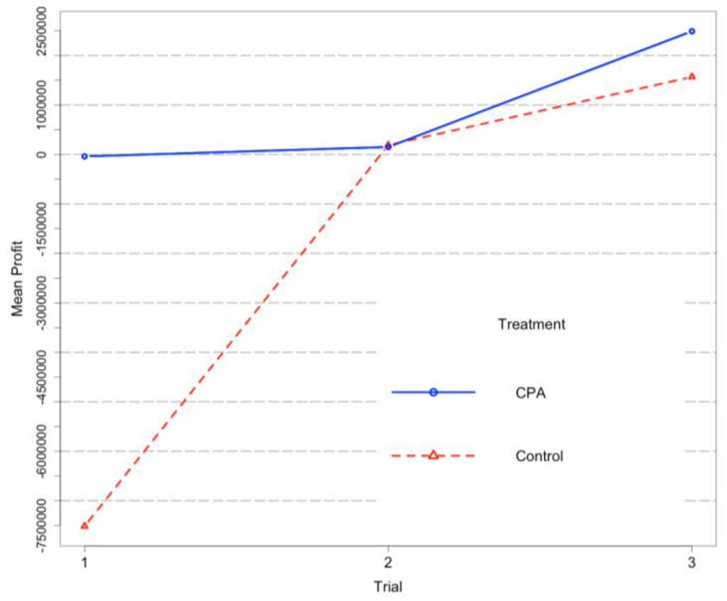
Figure 5.
Mean cumulative profit for the CPA group and the control group over all trials.
4.1. Test of Hypotheses
Given that the dependent variable was negatively skewed, a general linear model with a Poisson link function was estimated in order to test for the relationships proposed in the hypotheses. This allows for the accommodation of non-normal response distributions, as in the current analysis. Two subjects were excluded because of a very high divergence in their performance in the third round from the distribution. Their standardized performance was greater or near to −3. As a first step, the dependent variable was inverted. Following this, performance was fitted into a Poisson distribution, leading to 14 groups with a constant width of about one million. The Kolmogorov-Smirnov test for checking the assumption of a Poisson distribution is non-significant with D = 0.19 and p < 0.06.
Model 1 of Table 3 tests for the impact of the treatment, mental model accuracy, the number of previous economics lectures attended, the sum of earnings in former trials, and the time needed to perform all three trials.
Table 3.
Results of GLM for performance.
| Variables | Model 1 | ||
|---|---|---|---|
| Unstandardized B | Std. Error | Standardized β | |
| Intercept | 2.63 *** | 0.54 | |
| Treatment CPA | −0.40 * | 0.18 | −0.08 |
| Mental Model Accuracy | −0.02 * | 0.01 | −0.09 |
| Economics Lectures Attended | 0.03 ** | 0.01 | 0.09 |
| Total Performance in Trials 1 & 2 † | −0.01 | 0.01 | −0.06 |
| Total Time for Trials 1, 2, & 3 | −0.01 | 0.01 | −0.07 |
| Null Deviance | 78.00 on 45 degrees of freedom | ||
| Residual Deviance | 44.82 on 40 degrees of freedom | ||
| AIC | 185.15 | ||
† Performance scaled to one-million units;* p < 0.05; ** p < 0.01; *** p < 0.001.
Six subjects were excluded after performing the GLM regression. Given model 1, they had a large impact on results. Their impact was specified by the values of the Studentized residuals of above 3 or below −3, hat values of above three times the mean [41,42], and a Cook’s distance of near to or greater than one [43]. Assessing the residual deviance of model 1 using a Chi-squared test with 40 degrees of freedom leads to a non-significant result with p = 0.28, indicating a reasonable fit of the whole model.
On average, subjects in the CPA treatment reached a higher performance in comparison to the control group (B = −0.4, exp(B) = 0.67, p < 0.05). This supports Hypothesis 1, which asserts that the use of a structured method, i.e., the CPA cycle, leads to a higher performance. It is associated with a decrease of −0.4 in the log mean category of performance, while controlling for the other variables. Note that the scale of performance was inverted, so a lower category is related to a higher performance, and vice versa. To help interpret the effect, the coefficient was exponentiated to render it interpretable in the original scale. The use of a structured method leads to a multiplication of the performance category by 0.67, leading to an increased performance. The effect of mental model accuracy is significant (B = −0.02, exp(B) = 0.98, p < 0.05), indicating that an increase in an understanding of the underlying system leads to a higher performance. This supports Hypothesis 3. The number of economics lectures attended has a significant and negative effect on performance in the task (B = 0.03, exp(B) = 1.03, p < 0.01). The more such lectures that a subject has attended, the lower her performance. The performance in the first two learning trials and the time needed to perform all three trials were not significant predictors of performance in the final trial.
Table 4 shows the influence of the treatment, the time needed to answer the questionnaire for the mental model, the total performance for the first two trials, and the time needed to perform these trials on the score for mental model accuracy. Model 2 was estimated by using an ordinary least squares (OLS) regression. The treatment does not have a significant effect on mental model accuracy (B = −1.24, p > 0.66). Hypothesis 2 is therefore not supported. Significant predictors are the time needed to complete the questionnaire (B = 3.62, p < 0.001) and the overall performance of the learning trials (B = 0.45, p < 0.001). The time needed for these two trials is not significant.
As already outlined, to test Hypothesis 4, the guidelines of Baron and Kenny [44] and Kenny, Kashy, and Bolger [45] were followed. One additional model was necessary to cover the first step. The result of the GLM regression for performance without controlling for mental model accuracy is shown as Model 3 in Table 5. The existing models capture the other three steps.
The treatment, i.e., the independent variable, has a significant effect on performance, i.e., the dependent variable (B = −0.43, exp(B) = 0.65, p < 0.05). In comparison to Model 1, the total performance in trials 1 and 2 (B = −0.02, exp(B) = 0.98, p < 0.001) and the total time needed for all three trials become significant (B = −0.02, exp(B) = 0.98, p < 0.05). “Economics lectures attended” remains a significant predictor (B = 0.03, exp(B) = 1.04, p < 0.01). The strength of all effects is slightly greater when not controlling for mental model accuracy. The whole model shows an acceptable fit concerning the residual deviance. A Chi-squared test with 41 degrees of freedom leads to a non-significant result with p = 0.15. Because of the significant relationship between initial and outcome variable, Step 1 is met.
Table 4.
Results of OLS for mental model accuracy.
| Variables | Model 2 | ||
|---|---|---|---|
| Unstandardized B | Std. Error | Standardized β | |
| Intercept | 32.72 *** | 6.14 | |
| Treatment CPA | −1.24 | 2.79 | −0.05 |
| Time for Questionnaire | 3.62 *** | 0.76 | 0.53 |
| Total Performance in Trials 1 & 2 † | 0.45 *** | 0.12 | 0.42 |
| Total Time for Trials 1 & 2 | 0.02 | 0.13 | 0.02 |
| Adjusted R2 | 0.41 | ||
| F | 9.73 *** | ||
| Observations | 51 | ||
| Residual Standard Error | 9.52 on 46 degrees of freedom | ||
† Performance scaled to one-million units * p < 0.05; ** p < 0.01; *** p < 0.001.
Model 2 represents the necessary regression for Step 2 in the guideline. As discussed above, the CPA cycle does not have a significant effect on mental model accuracy. Step 2 is therefore not met. Since its being met is essential for establishing mediation, Hypothesis 4 is not supported. For the sake of completeness, the remaining two points are briefly discussed. Model 1 covers the third step. Mental model accuracy, as the potential mediator, is a significant predictor of performance. This fulfills the condition for Step 3. Simultaneously, the CPA cycle remains significant, and its effect size is only marginally diminished in comparison to Model 3. This result does not comply with the requirement of step 4 and is connected to the non-compliance of Step 2.
Table 5.
Results of GLM for performance without controlling for mental model accuracy.
| Variables | Model 3 | ||
|---|---|---|---|
| Unstandardized B | Std. Error | Standardized β | |
| Intercept | 1.86 *** | 0.43 | |
| Treatment CPA | −0.43 * | 0.18 | −0.09 |
| Economics Lectures Attended | 0.03 ** | 0.01 | 0.09 |
| Total Performance in Trials 1 & 2 † | −0.02 *** | 0.01 | −0.11 |
| Total Time for Trials 1, 2, & 3 | −0.02 * | 0.01 | −0.09 |
| Null Deviance | 78.00 on 45 degrees of freedom | ||
| Residual Deviance | 50.28 on 41 degrees of freedom | ||
| AIC | 188.62 | ||
† Performance scaled to one-million units; * p < 0.05; ** p < 0.01; *** p < 0.001.
4.2. Deep Structure
Model 4 in Table 6 shows the effect of deep structure understanding on performance. Model 3 uses the same independent variables as Model 1, with the difference being that mental model accuracy is split into two variables: deep structure and non-deep structure. The deep structure subscale had a Cronbach’s α = 0.65, while the non-deep structure, consisting of the remaining items, had a Cronbach’s α = 0.62. Both levels are low, but still acceptable [46]. Deep structure accuracy has a highly significant effect on performance (B = −0.02, exp(B) = 0.98, p < 0.001); non-deep structure is not significant. The estimated predictor of the number of economics lectures attended is significant and comparable to model 1. The other predictors are not significant. This includes the treatment effect of the structured method. The model itself shows a reasonable fit when assessing the residual deviance using a Chi-squared test with 39 degrees of freedom. The test is non-significant with p = 0.67.
Table 6.
Results of GLM for performance using deep structure.
| Variables | Model 4 | ||
|---|---|---|---|
| Unstandardized B | Std. Error | Standardized β | |
| Intercept | 2.14 *** | 0.54 | |
| Treatment CPA | −0.21 | 0.17 | −0.04 |
| Deep Structure | −0.02 *** | 0.00 | −0.20 |
| Non-Deep Structure | 0.01 | 0.01 | 0.05 |
| Economics Lectures Attended | 0.04 ** | 0.01 | 0.10 |
| Total Performance in Trials 1 & 2 † | −0.00 | 0.01 | −0.00 |
| Total Time for Trials 1 & 2 | −0.00 | 0.01 | −0.02 |
| Null Deviance | 84.38 on 45 degrees of freedom | ||
| Residual Deviance | 34.66 on 39 degrees of freedom | ||
| AIC | 178.44 | ||
† Performance scaled to one-million units; * p < 0.05; ** p < 0.01; *** p < 0.001.
4.3. Subject Demographics
It is possible that the demographics of the subjects who participated in the experiment will have had an influence on the results of this study and, therefore, on their generalizability. To analyze these potential factors, a generalized linear model has been estimated that relates performance to different demographic variables. Model 5 in Table 7 presents the results in which performance in the complex task is explained by age, gender, the number of economics lectures attended, prior work experience, as well as prior experiment participation and major field of study. A Chi-squared test with 36 degrees of freedom leads to a non-significant result with p = 0.09. The residual deviance is not significant at the five percent level, but the model should still be interpreted with caution due to the low p-value.
Table 7.
Results of GLM for performance using subject demographics.
| Variables | Model 5 | ||
|---|---|---|---|
| Unstandardized B | Std. Error | Standardized β | |
| Intercept | −0.19 | 0.90 | |
| Age | 0.02 | 0.03 | 0.02 |
| Gender | |||
| Female | −0.02 | 0.24 | −0.00 |
| Economics Lectures Attended | 0.04 * | 0.02 | 0.11 |
| Prior work experience a | 0.00 | 0.01 | 0.01 |
| Prior experiment participation | 0.59 * | 0.28 | 0.08 |
| Field of study b | |||
| Engineering | 0.83 | 0.54 | 0.17 |
| Industrial Engineering | 0.69 | 0.54 | 0.14 |
| Business/Management | 0.48 | 0.57 | 0.10 |
| Science | 0.78 | 0.66 | 0.11 |
| Null Deviance | 66.07 on 45 degrees of freedom | ||
| Residual Deviance | 48.16 on 36 degrees of freedom | ||
| AIC | 195.51 | ||
a Measured in months; b Implemented as dummy variables; * p < 0.05; ** p < 0.01; *** p < 0.001.
Only two variables were significant. As before, the number of economic lectures attended has a negative effect on performance (B = 0.04, exp(B) = 1.04, p < 0.05). If a subject had not participated in an experiment before the experiment presented in this study, her performance was significantly lower than that of experienced subjects (B = 0.59, exp(B) = 1.81, p < 0.05).
5. Discussion
5.1. Summary
Prior work has discussed systems thinking as a way of coping with complex systems and overcoming barriers to learning. For example, Richmond [6] and Sterman [7] propose possible requirements for improving learning in complex systems and eventually enhancing performance. Maani and Maharaj [30] empirically examined systems thinking in their experiment. Their results suggest that a specific pattern of behavior explains subjects’ performance. They called this structured method “CPA cycle”. However, besides Maani and Maharaj [30], further empirical studies are necessary to shed further light on systems thinking and its implications. In our study, an experiment was conducted to test for the impact of such a structured method on performance in a complex task.
Our results show that the use of the CPA cycle does have a positive effect on performance. This provides empirical evidence for the findings of Maani and Maharaj [30]. Using a structured method to cope with a complex system helps participants in their decision-making process. It enhanced the information processing capabilities of the subjects, eventually leading to a more efficient utilization of information [32]. Unlike in previous research, subjects learned how to use a general method of handling complex systems, and some of them did not make use of it in the first place. This implies the importance of learning, education, and experience when dealing with complex systems. This result is in accordance with previous studies. Sweeney and Sterman [8] conducted an experiment to test the knowledge of highly educated subjects about basic concepts of system dynamics and systems thinking. Subjects revealed a poor level of understanding. The authors conclude with a call for more education in system dynamics and systems thinking. In another experimental study, Doyle, Radzicki, and Trees [47] come to the conclusion that even a modest system dynamics intervention can promote learning.
The findings also show that mental model accuracy influences performance outcomes. This is consistent with prior research [2,3,17,18], suggesting that subjects with a better understanding of the underlying structure and causal relationships of the systems achieve a higher performance. In addition, our results indicate that a complete understanding of the system is not necessary. An accurate mental model of the deep structure, formed by key relationships, is sufficient to reach a higher performance. This is in line with the findings of Gary and Wood [17]. Knowledge of the environment is of high importance, but an understanding of the key links influencing the environment is even more important.
A relationship between the CPA cycle and mental model accuracy was not found. This may indicate that the CPA cycle does not improve learning and revision of mental models; therefore, it does not lead to an improved understanding of the structure of the task. The hypothesized mediation effect of the structured method on performance via the intermediate variable of mental model accuracy is, correspondingly, also not significant. This relationship was in addition separately analyzed, confirming this result. Why the use of the CPA cycle enhances performance in the experiment, but does not simultaneously improve mental model accuracy, remains unclear. A possible explanation may be the elicitation method of mental model accuracy that may conceal the effect. Alternatively, only a direct effect of the CPA cycle may exist, which works through enhancing the decision-making process itself.
Rather surprising is the negative effect of the number of economics lectures attended. Typically, the expectation is that knowledge of how companies work and how they are managed would be beneficial for achieving a high performance outcome. This should hold true for the task at hand, where the subjects had to manage a simulated company. That the opposite occurred, suggests that an economics background obstructs the open-mindedness of subjects. This leads to a bias in their decisions. They may expect aspects such as “marketing”, for example, to be of high relevance given their economics knowledge, while in the simulation it has less priority.
5.2. Limitations and Future Research
This study has some limitations which may reduce the significance of its conclusion. The first limitation may lie in the applied experimental method [48]. An experiment allows an environment to be controlled, leading to a high internal validity. On the other hand, the artificial situation may reduce the external validity. It would be of interest not only to repeat this study with other tasks in order to strengthen the generalizability of our results but also to test the CPA cycle in a different setting, such as in a classroom. A classroom experiment would enable an in-depth training that would incorporate other aspects of systems thinking. Further, the use of students as subjects, as in the experiment conducted for this research, may not be representative of the general population. Several studies discussed the use of students as subjects in laboratory experiments, arguing that incorporating students does inherently reduce external validity [49,50,51].
A bias between the two groups may result from differences concerning, for example, age, gender, or field of study. The composition of the two groups after random allocation was tested in relation to these three demographic variables. No significant differences were found. Additionally, the effect of several demographic variables on performance was analyzed, and two of them were significant. First, the already mentioned number of economics lectures attended, and second, prior participation in experiments. The latter may be explained by a level of insecurity about what to expect and how to behave in this new situation. This could have led to distraction and less concentration on the task at hand. It must be noted that this was for only four subjects the first experiment. Hence, this result should be interpreted with caution due to the small number of cases. The four subjects were spread evenly across the two groups. Other demographic factors, such as age, gender, or major field of study, do not have a significant impact on performance. These results do not support a gender effect in systems thinking, unlike that indicated in a study by Sweeney and Sterman [8]. However Sweeney and Sterman only found a marginally significant effect. A potential bias between the two groups, which may have resulted in a higher performance of the CPA group, was not found in the current study.
The focus of this research is on the general link between a structured method and complex decision-making. To fully understand the cause-effect relationships of the CPA cycle during decision-making and the reasons why it may not influence the mental model of subjects, further research is needed. This research should concentrate on the difference between the process of decision-making with and without using the CPA cycle. Additionally, changes in the mental models could allow a deeper insight into learning effects. Doyle, Radzicki, and Trees [47] described general features of a rigorous method to measure changes in mental models and also provided a detailed example of the application of the method. Limitations concerning the elicitation method may also relate to this study.
The elicitation method used to elicit the mental models of the participants should also be mentioned. The measure of mental model accuracy applied in this study does not include all possible elements of mental models, and also the procedures to measure and distinguish these elements need further research [16]. Another constraint is the degree of ability of participants to apply enhanced elicitation methods to mental models. The method used in this study was designed to be easy to use so that it would be applicable in an experimental setting. More elaborate procedures may be able to capture both the development of mental models over time and how a structured method may influence this development and, therefore, the learning process.
The proposed structured method—the CPA cycle—is not the only one discussed in the literature. Sterman [7], for example, mentions the PDCA cycle (Plan–Do–Check–Act) used in improvement processes of total quality management [52]. The DMAIC approach (Define–Measure–Analyze–Improve–Control) in Six Sigma should likewise be mentioned in this context [53]. A comparison of these methods could give insights into the relevance of different parts of the procedures and would increase the generalizability of the results.
The results of this study support the notion of “heuristic competence” being a general capability of coping with complex systems. We have shown that subjects can be taught to use a structured method, i.e., the CPA cycle, which improves their performance. This has implications for future research in the field of systems thinking and education in system dynamics.
Acknowledgments
This research was funded by the Deutsche Forschungsgemeinschaft (DFG) via the Graduiertenkolleg 1491: Anlaufmanagement—Entwicklung von Entscheidungsmodellen im Produktionsanlauf. The author would like to thank the reviewers for their useful and constructive comments.
Conflicts of Interest
The author declares no conflict of interest. The funding sponsors had no role in the design of the study; in the collection, analyses, or interpretation of data; in the writing of the manuscript, and in the decision to publish the results.
Appendix A. Instructions on and Examples of the Questions about Causal Relationships (Translated from the German)
So that we can measure your understanding of the system in this simulation, we would kindly ask you to answer the following 25 questions. These questions refer to possible relationships between variables in the simulation. The questions all take the following form:
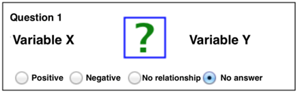
Please indicate whether there is a relationship between the stated variables by referring to your understanding of the system at hand. Does the left variable (‘X’) have a positive, negative, or no influence on the variable on the right (‘Y’)? Please use only your knowledge about the simulation. Focus exclusively on direct relationships and ignore any intervening variables. Indirect relationships are not relevant.
Explanation of the Different Relationships
- ○
- Positive: The variable X has a positive influence on variable Y. An increase of X leads to an increase of Y, all else being equal. A decrease in X leads to a decrease in Y, all else being equal. X and Y move in the same direction.
- ○
- Negative: The variable X has a negative influence on variable Y. An increase of X leads to a decrease of Y, all else being equal. A decrease in X leads to an increase in Y, all else being equal. X and Y move in the opposite direction.
- ○
- No relationship: There is no direct relationship between these variables. Any change to variable X has no influence on variable Y.
- ○
- No Answer: If you are unsure about the answer, please use this option rather than simply making a guess.
| Question No. | Variable X | Variable Y |
| Question 4 | Stock | Storage Costs |
| Question 9 | Number of machines | Fixed Costs |
| Question 17 | Price | Sales |
| Question 18 | Time | Incoming Orders |
| Question 24 | Cumulative Production | Variable Costs |
References
- Größler, A.; Maier, F.H.; Milling, P.M. Enhancing learning capabilities by providing transparency in business simulators. Simul. Gaming 2000, 31, 257–278. [Google Scholar] [CrossRef]
- Capelo, C.; Dias, J.F. A system dynamics-based simulation experiment for testing mental model and performance effects of using the balanced scorecard. Syst. Dyn. Rev. 2009, 25, 1–34. [Google Scholar] [CrossRef]
- Ritchie-Dunham, J.L. Balanced Scorecards, Mental Models, and Organizational Performance. Ph.D. Thesis, Department of Management Science and Information Systems, University of Texas at Austin, Austin, TX, USA, 2002. [Google Scholar]
- Rouwette, E.A.; Größler, A.; Vennix, J.A. Exploring influencing factors on rationality: A literature review of dynamic decision-making studies in system dynamics. Syst. Res. Behav. Sci. 2004, 21, 351–337. [Google Scholar] [CrossRef]
- Sengupta, K.; Abdel-Hamid, T.K. Alternative conceptions of feedback in dynamic decision environments: An experimental investigation. Manag. Sci. 1993, 39, 411–428. [Google Scholar] [CrossRef]
- Richmond, B. Systems thinking: Critical thinking skills for the 1990s and beyond. Syst. Dyn. Rev. 1993, 9, 113–133. [Google Scholar] [CrossRef]
- Sterman, J.D. Learning in and about complex systems. Syst. Dyn. Rev. 1994, 10, 291–233. [Google Scholar] [CrossRef]
- Sweeney, L.B.; Sterman, J.D. Bathtub dynamics: Initial results of a systems thinking inventory. Syst. Dyn. Rev. 2000, 16, 249–286. [Google Scholar] [CrossRef]
- Brehmer, B. Dynamic decision making: Human control of complex systems. Acta Psychol. 1992, 81, 211–241. [Google Scholar] [CrossRef]
- Sterman, J.D. Modeling managerial behavior: Misperceptions of feedback in a dynamic decision making experiment. Manag. Sci. 1989, 35, 321–339. [Google Scholar] [CrossRef]
- Paich, M.; Sterman, J.D. Boom, bust, and failures to learn in experimental markets. Manag. Sci. 1993, 39, 1439–1458. [Google Scholar] [CrossRef]
- Moxnes, E. Misperceptions of basic dynamics: The case of renewable resource management. Syst. Dyn. Rev. 2004, 20, 139–162. [Google Scholar] [CrossRef]
- Sterman, J.D. Does formal system dynamics training improve people’s understanding of accumulation? Syst. Dyn. Rev. 2010, 26, 316–334. [Google Scholar] [CrossRef]
- Cronin, M.A.; Gonzalez, C. Understanding the building blocks of dynamic systems. Syst. Dyn. Rev. 2007, 23, 1–17. [Google Scholar] [CrossRef]
- Jones, N.; Ross, H.; Lynam, T.; Perez, P.; Leitch, A. Mental models: An interdisciplinary synthesis of theory and methods. Ecol. Soc. 2011, 16, 6. [Google Scholar]
- Grösser, S.N.; Schaffernicht, M. Mental models of dynamic systems: Taking stock and looking ahead. Syst. Dyn. Rev. 2012, 28, 46–68. [Google Scholar] [CrossRef]
- Gary, M.S.; Wood, R.E. Mental models, decision rules, and performance heterogeneity. Strateg. Manag. J. 2011, 32, 569–594. [Google Scholar] [CrossRef]
- McNamara, G.M.; Luce, R.A.; Tompson, G.H. Examining the effect of complexity in strategic group knowledge structures on firm performance. Strateg. Manag. J. 2002, 23, 153–117. [Google Scholar] [CrossRef]
- Langley, P.A. Building cognitive feedback into a microworld learning environment: Results from a pilot experiment. In Proceedings of the 1995 International System Dynamics Conference, System Dynamics’ 95, Tokyo, Japan, 30 July – 4 August 1995; pp. 628–637.
- Howie, E.; Sy, S.; Ford, L.; Vicente, K.J. Human-computer interface design can reduce misperceptions of feedback. Syst. Dyn. Rev. 2000, 16, 151–171. [Google Scholar] [CrossRef]
- Senge, P.M. The Fifth Discipline: The Art and Practice of the Learning Organization, 1st ed.; Doubleday: New York, NY, USA, 2006. [Google Scholar]
- Checkland, P. Systems Thinking, Systems Practice: Includes a 30-Year Retrospective, 1st ed.; John Wiley & Sons: Chichester, UK, 1999. [Google Scholar]
- Gharajedaghi, J. Systems Thinking: Managing Chaos and Complexity: A Platform for Designing Business Architecture, 1st ed.; Butterworth-Heinemann: Woburn, MA, USA, 1999. [Google Scholar]
- Frank, M. Engineering Systems Thinking and Systems Thinking. Syst. Eng. 2000, 3, 163–168. [Google Scholar] [CrossRef]
- Valerdi, R.; Rouse, W.B. When Systems Thinking is Not a Natural Act. In Proceedings of the 2010 4th Annual IEEE Systems Conference, San Diego, CA, USA, 5–8 April 2010; pp. 184–189.
- Pan, X.; Valerdi, R.; Kang, R. Systems Thinking: A Comparison between Chinese and Western Approaches. Procedia Comput. Sci. 2013, 16, 1027–1035. [Google Scholar] [CrossRef]
- Bosch, O.J.H.; King, C.A.; Herbohn, J.L.; Russell, I.W.; Smith, C.S. Getting the Big Picture in Natural Resource Management—Systems Thinking as “Method” for Scientists, Policy Makers and Other Stakeholders. Syst. Res. Behav. Sci. 2007, 24, 217–232. [Google Scholar] [CrossRef]
- Bosch, O.J.H.; Nguyen, N.C.; Maeno, T.; Yasui, T. Managing Complex Issues through Evolutionary Learning Laboratories. Syst. Res. Behav. Sci. 2013, 30, 116–135. [Google Scholar] [CrossRef]
- Doyle, J.K. The Cognitive Psychology of Systems Thinking. Syst. Dyn. Rev. 1997, 13, 253–265. [Google Scholar] [CrossRef]
- Maani, K.E.; Maharaj, V. Links between systems thinking and complex decision making. Syst. Dyn. Rev. 2004, 20, 21–48. [Google Scholar] [CrossRef]
- Todd, P.; Benbasat, I. Process tracing methods in decision support systems research: Exploring the black box. MIS Q. 1987, 11, 493–512. [Google Scholar] [CrossRef]
- Letmathe, P.; Zielinski, M. Determinants of feedback effectiveness in production planning. (In preparation)
- Maani, K.; Cavana, R.Y. Systems Thinking, System Dynamics: Managing Change and Complexity, 2nd ed.; Pearson Education: Auckland, New Zealand, 2007. [Google Scholar]
- Crawley, M.J. The R Book, 2nd ed.; John Wiley & Sons: Chichester, UK, 2012. [Google Scholar]
- Letmathe, P.; Schweitzer, M.; Zielinski, M. How to learn new tasks: Shop floor performance effects of knowledge transfer and performance feedback. J. Oper. Manag. 2012, 30, 221–236. [Google Scholar] [CrossRef]
- Edmondson, A.C.; Winslow, A.B.; Bohmer, R.M.J.; Pisano, G.P. Learning how and learning what: Effects of tacit and codified knowledge on performance improvement following technology adoption. Decis. Sci. 2003, 34, 197–224. [Google Scholar] [CrossRef]
- Markíczy, L.; Goldberg, J. A method for eliciting and comparing causal maps. J. Manag. 1995, 21, 305–333. [Google Scholar] [CrossRef]
- Hodgkinson, G.P.; Maule, A.J.; Bown, N.J. Causal cognitive mapping in the organizational strategy field: A comparison of alternative elicitation procedures. Organ. Res. Methods 2004, 7, 3–26. [Google Scholar] [CrossRef]
- Kabacoff, R.I. R in Action: Data Analysis and Graphics with R, 1st ed.; Manning Publication: New York, NY, USA, 2011. [Google Scholar]
- Venables, W.N.; Ripley, B.D. Modern Applied Statistics with S, 4th ed.; Springer: Berlin, Germany, 2002. [Google Scholar]
- Stevens, J.P. Applied Multivariate Statistics for the Social Sciences, 5th ed.; Routledge: London, UK, 2012. [Google Scholar]
- Field, A.; Miles, J.; Field, Z. Discovering Statistics Using R, 1st ed.; Sage Publications: Los Angeles, CA, USA, 2012. [Google Scholar]
- Cook, R.D.; Weisberg, S. Residuals and Influence in Regression, 1st ed.; Chapman and Hall: London, UK, 1982. [Google Scholar]
- Baron, R.M.; Kenny, D.A. The moderator-mediator variable distinction in social psychological research: Conceptual, strategic, and statistical considerations. J. Personal. Soc. Psychol. 1986, 51, 1173–1182. [Google Scholar] [CrossRef]
- Kenny, D.A.; Kashy, D.A.; Bolger, N. Data analysis in social psychology. In Handbook of Social Psychology 1, 4th ed.; Gilbert, D.T., Fiske, S.T., Lindzey, G., Eds.; McGraw-Hill: New York, NY, USA, 1998; pp. 233–265. [Google Scholar]
- DeVellis, R.F. Scale Development: Theory and Applications, 3rd ed.; Sage Publications: Los Angeles, CA, USA, 2012. [Google Scholar]
- Doyle, J.K.; Radzicki, M.J.; Trees, W.S. Measuring Change in Mental Models of Complex Dynamic Systems. In Complex Decision Making: Theory and Practice, 1st ed.; Qudrat-Ullah, H., Spector, M.J., Davidsen, P., Eds.; Springer: Berlin, Germany, 2008; pp. 269–294. [Google Scholar]
- Falk, A.; Heckman, J.J. Lab Experiments Are a Major Source of Knowledge in the Social Sciences; CESifo Working Paper, No. 2894; ZBW—Leibnitz Information Centre for Economics: Kiel, Germany, 2009. [Google Scholar]
- Benz, M.; Meier, S. Do People Behave in Experiments as in the Field? Evidence from Donations; Federal Reserve Bank of Boston, Working Paper, No. 06-8; ZBW—Leibnitz Information Centre for Economics: Kiel, Germany, 2006. [Google Scholar]
- Berkowitz, L.; Donnerstein, E. External validity is more than skin deep: Some answers to criticisms of laboratory experiments. Am. Psychol. 1982, 37, 245–257. [Google Scholar] [CrossRef]
- Druckman, J.N.; Kam, C.D. Students as experimental participants: A defense of the “Narrow Data Base”. In Cambridge Handbook of Experimental Political Science, 1st ed.; Druckman, J.N., Green, D.P., Kuklinski, J.H., Lupia, A., Eds.; Cambridge University Press: Cambridge, UK, 2011; pp. 41–57. [Google Scholar]
- Sokovic, M.; Pavletic, D.; Pipan, K.K. Quality improvement methodologies—PDCA cycle, RADAR matrix, DMAIC and DFSS. J. Achiev. Mater. Manuf. Eng. 2010, 43, 476–483. [Google Scholar]
- De Mast, J.; Lokkerbol, J. An analysis of the Six Sigma DMAIC method from the perspective of problem solving. Int. J. Prod. Econ. 2012, 139, 604–614. [Google Scholar] [CrossRef]
© 2015 by the author; licensee MDPI, Basel, Switzerland. This article is an open access article distributed under the terms and conditions of the Creative Commons Attribution license (http://creativecommons.org/licenses/by/4.0/).