From Reactive Response to Proactive Mitigation: The Value of Precursor Risk Signals in DRL Inventory Control

Highlights

Please indicate how your work links to systems science via your contributions to systems practice, theory, and/or methodology.

• A supply chain under disruption is modeled as a control system in which precursor risk signals add a feedforward path to the feedback loop of conventional replenishment.
• Signal quality and predictive horizon are treated as design parameters through which the value of advance supply information is quantified.

What are the main findings and/or the implications of the main findings?

• A precursor signal is valuable even when it is imperfect: a detection rate above about one half already pays, and at three quarters it yields a cost saving of 9% against a calibrated (s, Q) policy and 12% against a reactive DRL policy.
• The learned policy operates a state-dependent reorder point that stays low in calm periods and rises with the severity and proximity of a predicted disruption, and a transparent signal-triggered reorder-point rule captures about 83% of the gain.

Abstract

Modern supply chains face abrupt supply disruptions, under which the stable lead time assumption behind conventional inventory control no longer holds. Most replenishment models, including existing deep reinforcement learning (DRL) formulations, act as feedback controllers. A disruption is treated as an unobservable event, and correction begins only after deliveries are already delayed. In practice, however, disruptions are often preceded by observable precursor signals. This paper develops a risk sensing DRL framework that incorporates such signals into the state of a proximal policy optimization (PPO) agent, introducing feedforward control into the replenishment decision. The signal quality (detection rate) and the predictive horizon are treated as explicit design parameters. In a two-echelon system with graded disruptions, the risk sensing policy achieves substantial cost savings against both a per-environment calibrated (s, Q) policy and an identically trained reactive DRL policy, even with an imperfect signal. The required horizon is short, as horizons longer than needed bring no further gain. In contrast, the savings depend critically on the signal quality, as a meaningful gain over the calibrated benchmark requires a signal that detects well over half of upcoming disruptions. The advantage is greatest where severe disruptions are infrequent. The learned policy operates a state-dependent reorder point that stays low in calm conditions and rises with the severity and proximity of a predicted threat. A transparent rule driven by the same signal captures about 83% of the gain, indicating that most of the value comes from the information itself rather than from the learning method. These results quantify the value of advance supply information in inventory control and show how it supports the transition from reactive response to proactive mitigation.

1. Introduction

In recent years, supply chains have become increasingly exposed to abrupt, large-scale disruptions that arise from diverse sources, including geopolitical instability, port congestion, and other logistical bottlenecks. For example, following the military escalation around the Strait of Hormuz in early 2026, transits through the strait fell sharply and some 2000 vessels were stranded [1], immobilizing a large share of global crude oil shipments and forcing the remaining flows onto longer and less predictable routes [2,3]. Under such disruptions, the assumptions of stable lead times and reliable supply in conventional inventory models no longer hold. Classical replenishment policies such as the continuous-review (r, Q) policy are effective under stationary conditions, but their control parameters, in particular the reorder point, are determined for a stationary lead time distribution. During major supply-side shocks, a reorder point calibrated to cover demand over the normal lead time can no longer function as intended. The policy has no mechanism to incorporate information about an impending disruption, so it cannot respond until the shock has already taken effect. By then, severe stockouts are unavoidable and total system costs increase sharply.

These limitations have motivated growing interest in deep reinforcement learning (DRL) for inventory problems that are difficult to solve with classical methods. Most DRL applications, however, share the same reactive limitation. The state is typically confined to internal variables such as on-hand inventory and outstanding pipeline orders, with supply uncertainty represented as a stationary distribution rather than as something the agent can anticipate [4]. Such an agent cannot foresee an impending shock and revises its policy only once lead times have already lengthened.

In practice, supply disruptions are often preceded by observable signals such as weather forecasts, port-congestion indices, or supplier risk alerts that become available before the disruption is realized. Augmenting the agent’s state with such exogenous information has been noted as a promising research direction [4]. Recent studies have begun to bring exogenous information into the state, but almost exclusively on the demand side, in the form of demand histories, forecasts, and related covariates [5,6]. Advance information about the supply side has remained unexplored. We propose a risk sensing DRL framework that incorporates precursor risk signals into the state space of a PPO agent, thereby introducing a feedforward component into the replenishment decision. The agent learns to map these signals to adjustments in reorder timing and to position protective inventory ahead of a disruption. The value of this mechanism depends on the reliability of the signals and the length of the prediction window they provide. We therefore treat signal quality and predictive horizon as explicit design parameters rather than assuming perfect foresight. Preparing an organization for disruptions before they occur is also the purpose of scenario planning, the established managerial approach to this problem. The model developed here operates at a different level, and Section 8 discusses how the two complement each other.

These considerations lead to three research questions.

RQ1.

Does incorporating precursor risk signals into the state of a DRL agent reduce the long-run cost of inventory control, relative to a calibrated static policy and to an identically trained reactive policy?

RQ2.

How does the value of the signal depend on its quality and on the predictive horizon? How reliable and how early must a warning be to be worth acting on?

RQ3.

How much of the measured value comes from the information itself rather than from learning, and through what mechanism does the policy convert warnings into cost savings?

The contributions of this paper are as follows. First, we extend the conventional DRL state representation to incorporate observable precursor risk signals. Second, we develop a PPO-based learning scheme that maps these signals to proactive reorder decisions. Third, by treating signal quality and predictive horizon as design parameters, we measure the value of advance information directly, quantifying how cost and service-level performance improve as more and better information becomes available, relative to a conventional (s, Q) policy.

2. Related Work

2.1. Inventory Control Under Stochastic Lead Times

Classical inventory models treated lead times as deterministic or stationary quantities. As global supply chains grew more complex and supply-side risk became a prominent operational concern, interest in lead time uncertainty increased, and a substantial body of work extended the traditional continuous-review (r, Q) and periodic review (s, S) policies to stochastic lead times.

Kaplan [7] established the dynamic-programming formulation for random lead times under the assumption that orders do not cross in time, which was elaborated in subsequent work [8,9]. Later studies extended the analysis to broader lead time distributions [10] and to environments allowing order crossovers [11]. Song [12] further showed that greater lead time variability raises the long-run average cost.

These frameworks, however, share the assumption that the lead time distribution is stationary and can be estimated from historical data. When the supply process undergoes a structural break, parameters calibrated to past observations no longer describe future supply, and a policy derived under stationarity has no mechanism to adapt once that assumption fails.

2.2. DRL Applications in Inventory Management

Deep reinforcement learning (DRL) has emerged as a data-driven approach to inventory control in such disrupted settings. By learning policy mappings directly through interaction with the environment, DRL agents avoid the restrictive distributional assumptions of classical models, and the approach has been applied to several problems that are intractable for exact methods. Oroojlooyjadid et al. [13] used deep Q-networks in a serial multi-echelon beer game. Without prior knowledge of the demand distribution, their agent learned near-optimal ordering policies when the other agents followed base-stock policies and remained superior when they behaved irrationally. Gijsbrechts et al. [14] applied an asynchronous advantage actor–critic (A3C) algorithm to lost-sales, dual-sourcing, and multi-echelon problems, and found that it can match the performance of state-of-the-art heuristics and approximate dynamic programming methods. DRL has since been extended to a range of other settings, such as capacitated lot sizing under non-stationary demand [15] and the integration of demand forecasts [16]. Recent studies have begun to incorporate exogenous information into these formulations, but mostly on the demand side. Madeka et al. [5] learn replenishment policies whose inputs include historical demand and related covariates, and Alvo et al. [6] optimize policies on real demand series across inventory networks. DRL has also been applied to systems under supply disruptions, but in a reactive form, where the state carries the current disruption status and the policy responds only after a disruption is realized [17]. On the algorithmic side, Stranieri et al. [18] compare several algorithms in a two-echelon system and report that PPO performs most consistently, and Temizöz et al. [19] develop a method tailored to the structure of inventory problems.

Existing studies, however, typically define the state over internal variables such as on-hand inventory and outstanding pipeline orders, without representing advance information about an impending disruption [4]. An agent restricted to internal state cannot anticipate the disruption and can react only after the pipeline has drained. The reactive limitation of classical policies thus persists in the data-driven setting.

2.3. Value of Advance Information and State Space Augmentation

The value of advance information is well established in inventory theory. Hariharan and Zipkin [20] showed that advance demand information substitutes for inventory, shortening the effective lead time and lowering the stock needed for a given service level. Gallego and Özer [21] showed that once the state is extended to include known future orders, state-dependent (s, S) and base-stock policies remain optimal, while Gavirneni et al. [22] quantified the value of downstream information sharing in a capacitated supplier–retailer system, showing that the supplier’s cost falls as more information becomes available.

Although these studies concern demand-side information under stationary conditions, the same principle applies to the supply side. An early study by Song and Zipkin [23] modeled the supply system as a Markov process that governs the lead time and showed that the optimal policy is state-dependent, with parameters that respond to the supply condition. Their model, however, relies on the current supply state rather than an advance warning. Such advance warnings are often available in practice, as a disruption is frequently preceded by observable risk signals. An agent that senses these signals gains time to respond before deliveries are actually delayed, securing protective inventory or reordering earlier. This enables a move from reactive recovery toward proactive adaptation, in line with the viability perspective of Ivanov [24].

Exploiting such signals, however, requires them to be included in an agent’s state, which the streams reviewed above have not addressed. The stochastic lead time literature treats lead time uncertainty as a stationary distribution to be estimated from history rather than as events to be anticipated. DRL studies incorporate exogenous information mostly on the demand side, through histories, forecasts, and covariates (Section 2.2), and the supply side has remained unexplored. Work on supply-risk information conditions the policy on the current supply state rather than on predicted future states. The supply chain risk literature, in turn, classifies disruptions by cause and by the shape of their unfolding [25,26], but does not connect these classes to the state of a replenishment policy. Section 3 makes this connection before the model is formulated. This study fills the gap by incorporating precursor risk signals into the state of a PPO agent, so that the replenishment policy anticipates disruptions instead of reacting to them, and by quantifying the resulting gain in cost and service-level performance.

3. Problem Description

This study is abstracted from the component replenishment practice of a large Korean electronics manufacturer. Key components such as displays and secondary batteries are sourced from strategic single suppliers, and a shortage of any of them halts assembly. To manage the risk of such shortages, the manufacturer has operated a supply risk management process for a number of years, in which disruptions are classified by their source, whether exogenous, internal to the supplier, or logistical, graded by their severity, and recorded with their causes and their impact on each product. Within this process, leading indicators of supply conditions are monitored, and the detection accuracy and the horizon of the resulting warnings are tracked as measures of monitoring performance. The question this study addresses is how such warnings should be used in responding to disruptions.

Supply disruptions arise from many causes and differ in their effects. Ports close because of storms, congestion, or conflict, and shipments wait or take longer routes. Supplier plants stop because of labor disputes, fires, or earthquakes, and production resumes only after settlement or repair. A failure at a sub-tier supplier (the supplier’s own suppliers at any tier beyond the first) propagates the disruption downstream, and customs and transport delays occur routinely. Chopra and Sodhi [25] classify supply chain risks into categories, each with its own drivers, and Sheffi and Rice [26] describe a disruption as a profile that unfolds in phases from preparation through impact to recovery, whose shape differs by type.

Table 1. Disruption types and their representation in the model.

Disruption Type (Example)	Effect on the Supplier’s Deliveries	Leading Indicators and Their Source	How Early It Becomes Recognizable	Representation in the Model
Port closure or route diversion (Strait of Hormuz, 2026)	Long delay while shipments wait or take longer routes	Conflict reports, shipping advisories, congestion indices; public sources and monitoring services	Gradual; visible days to weeks ahead	Severe grade; high detection rate; long horizon
Supplier plant stoppage, labor dispute	Long delay; production resumes after settlement	Dispute escalation, strike notice; the supplier itself	Gradual; typically announced	Severe grade; high detection rate
Supplier plant stoppage, fire or earthquake	Long delay; recovery depends on damage	Little or none	Sudden	Severe grade; low detection rate (mostly missed)
Sub-tier supplier failure	Delay at the immediate supplier once its own stock is exhausted	Low visibility; sometimes relayed by the supplier	Gradual but late to become visible	Intermediate grade; low detection rate; short horizon
Export control or regulatory hold	Long delay while clearance is obtained	Policy announcements; public sources	Gradual	Severe grade; medium detection rate
Customs or transport delay	Short delay	Carrier notices, port indices	Sudden or gradual	Mild grade; any detection rate

lists the main types. The responses available to a manufacturer are also diverse. Tomlin [27] distinguishes mitigation tactics taken before a disruption, such as holding protective inventory and qualifying a second source, from contingency tactics taken after it, such as rerouting and expediting shipments. Tang [28] surveys a broader set that includes postponement and flexible supply bases. This study considers protective inventory, which applies across disruption types and can be implemented at the operational level without changing the structure of the supply chain. The other responses are established risk management strategies but lie beyond the scope of the model, and Section 8 discusses what this restriction means for the results and their implications.

The decision is then when to place a fixed-lot order for the component with its supplier, and the disruptions above take effect on this decision as a lengthening of the delivery lead time. Deliveries from the supplier are delayed while the disruption lasts and resume when it is over, so that a disruption appears to the planner as an interruption of replenishment followed by recovery. The model assumes that the supplier continues to accept orders during the interruption and delivers them after it ends, an assumption stated with its scope in Section 4.1. A stoppage at the supplier’s plant, whether from a strike, a fire, or a failure further upstream, is represented in this way, since orders placed during the stoppage are queued and delivered once production resumes. Among the types in Table 1, this holds except where a regulatory hold bars the product itself, in which case orders are rejected rather than delayed.

Within this response, what distinguishes one disruption type from another is how long deliveries are delayed, whether the disruption can be recognized before it begins, and how early it becomes recognizable. The length of the interruption determines how severe a disruption is for replenishment, since it sets how many periods of demand must be covered without deliveries, and we refer to this severity as the grade of the disruption. Whether and how early a disruption is recognized depends on the leading indicators that precede it, which come from the supplier itself, through advance notices, and from public and commercial sources, such as port authorities, weather services, and supplier risk monitoring services. The prediction that such indicators support is what Section 4.2 defines as the precursor risk signal. We refer to the fraction of disruptions that such indicators reveal before the disruption onset as the detection rate, and to the number of periods between recognition and the disruption onset as the predictive horizon, since the earlier a disruption is recognized, the more time the planner has to build up stock. Table 1 places the main disruption types on these dimensions. The model of Section 4 formalizes these dimensions. The grade and its frequency define the disruption process (Section 4.1), and the detection rate and the predictive horizon define the signal (Section 4.2). Different disruption types are therefore represented as different positions on these dimensions rather than as a single event, and the learned policy responds to them differently, as Section 7.3 shows. Which of these types apply to a given manufacturer and what grade and detection rate each warrants is a judgment about the firm’s own exposure. Scenario planning is designed to support such judgments, and Section 8 discusses how it and the model studied here combine.

The model represents two parties, the manufacturer and its direct supplier. For a key component, the tiers above the direct supplier are monitored as well, because a disruption further upstream reaches the manufacturer only after it has propagated to a delay at the direct supplier, and watching the upstream tier reveals it that much earlier. The signal studied here does not restrict where the warning comes from. A warning obtained from an upstream tier is represented as a signal that detects the coming delay earlier, that is, with a longer predictive horizon, and the results of Section 7.2 on the value of the horizon apply to it. What the model does not represent is the propagation of a disruption from an upstream tier to the direct supplier. Thus, decisions that depend on how a disruption propagates through the supply network, such as which tiers to monitor, how to integrate warnings that arrive from different tiers, and where along the chain to position protective stock, lie outside its scope and are identified as future research in Section 9.

The disruptions in Table 1 act on the inbound side of the manufacturer. The same causes, such as a port closure, a transport strike, or a regional conflict, often disrupt its outbound logistics as well, delaying or losing sales and stranding finished products. When both sides are disrupted, the effects compound. The model studied here accounts only for the holding and shortage costs of the component and holds its demand stationary to isolate the effect of supply-side information (Section 6.1). It has no representation of outbound conditions, so outbound disruptions lie outside the model, as stated in Section 8, and the results should be read as the value of advance supply information on the inbound side, taken in isolation from outbound conditions.

4. Model Formulation

4.1. Inventory System and Disruption Dynamics

We consider a serial two-echelon supply chain consisting of a manufacturer and a supplier. The manufacturer (node 0) replenishes a component from a single supplier (node 1), which is itself supplied by an exogenous raw material source with infinite capacity and a constant lead time. The supplier is exposed to supply risk characterized by a risk profile specified below. We focus on inventory control at the manufacturer, where holding and shortage costs are incurred.

Table 2. Notation.

Symbol	Meaning
t	Review period index
$D\left(t\right)$, $\lambda$	Demand in period t; mean demand
Q	Fixed order quantity
s	Reorder point of the static benchmark
$\mathit{IL}\left(t\right)$, $\mathit{IT}\left(t\right)$, $\mathit{IP}\left(t\right)$	Inventory level; in-transit inventory; inventory position
$\mathit{RP}\left(t\right)$, $o\left(t\right)$	Arrivals in period t; pipeline vector of scheduled arrivals
h, p	Holding cost; shortage cost (per unit per period)
$\tau$	Normal lead time
g, G	Disruption severity grade; number of grades ($g=0$ normal)
${\beta }_g$, ${\Delta }_g$	Occurrence probability and added delay of grade g
${\Delta }_{\max }$	Maximum added delay
$\rho \left(t\right)$	Remaining length of the active disruption
$L\left(t\right)$	Total lead time of an order placed in period t
H	Predictive horizon
$\alpha$	Signal quality (detection probability of an upcoming disruption)
$\delta \left(t\right)$, $e\left(t\right)$	Realized delay and elapsed time of the active disruption
$\widehat{\delta }(t+i\mid t)$, $\widehat{e}(t+i\mid t)$	Predicted delay and elapsed time for period $t+i$
$a\left(t\right)$	Action: place order (1) or wait (0)
$\gamma$	Discount factor

summarizes the notation used in this paper.

Time is divided into review periods indexed by t. Demand $D\left(t\right)$ at the manufacturer is independent and identically distributed across periods with mean $\lambda$, and unsatisfied demand is backordered. Orders are placed in fixed lots of size Q, at most one lot per period, following the manufacturer’s material requirements planning. Let $\mathit{IL}\left(t\right)$ denote the inventory level (on-hand stock minus backorders) and $\mathit{IT}\left(t\right)$ the in-transit inventory. The inventory position is defined as

$$\mathit{IP}\left(t\right)=\mathit{IL}\left(t\right)+\mathit{IT}\left(t\right).$$

(1)

The cost incurred at the manufacturer in a period combines holding and shortage components,

$$C\left(t\right)=h\mathit{IL}{\left(t\right)}^{+}+h\mathit{IT}\left(t\right)+p\mathit{IL}{\left(t\right)}^{-},$$

(2)

where $x^{+}=\max (x,0)$ and $x^{-}=\max (-x,0)$. Here h is the holding cost per unit per period charged on on-hand and in-transit stock, and p is the shortage cost per unit per period charged on backorders. Broader formulations additionally consider ordering and transportation costs [29]. These are omitted here because, with a fixed lot size and backordered demand, every policy orders the same number of lots per period in the long run, so a per-lot ordering or transportation cost adds the same constant to every policy and does not affect the comparison.

Disruptions are modeled through a supplier risk profile. The supplier is subject to disruptions of G severity grades indexed by $g\in \{1,\dots ,G\}$ in decreasing order of severity, so that $g=1$ is the most severe grade and $g=G$ the least severe. The normal, undisrupted condition is denoted $g=0$. In each period, a disruption event of grade g occurs independently with probability ${\beta }_g$ and lasts for ${\Delta }_g$ consecutive periods. More damaging disruptions are rarer, so that ${\Delta }_1>\cdots >{\Delta }_G$ and ${\beta }_1<\cdots <{\beta }_G$.

The supplier’s disruption status is summarized by the remaining disruption length $\rho \left(t\right)$, with a disruption active whenever $\rho \left(t\right)>0$. A new event takes effect only if it outlasts what remains of the disruption in progress; otherwise, it is absorbed without effect:

$$\rho \left(t\right)=\left\{\begin{array}{cc}{\Delta }_g\hfill & \mathrm{if}\mathrm{a}\mathrm{grade}-g\mathrm{event}\mathrm{occurs}\mathrm{in}\mathrm{period}t\hfill \\ \hfill & \mathrm{and}{\Delta }_g>\max \left(\rho (t-1)-1,0\right),\hfill \\ \max \left(\rho (t-1)-1,0\right)\hfill & \mathrm{otherwise}.\hfill \end{array}\right.$$

(3)

In the first case the event overrides the disruption in progress, so the active grade becomes g and the onset is reset. A grade-g disruption that is not overridden lasts exactly ${\Delta }_g$ periods. The elapsed time $e\left(t\right)$ counts the periods since the onset of the active disruption and the realized delay $\delta \left(t\right)={\Delta }_g$ identifies its grade.

An order placed in period t is delivered after the total lead time

$$L\left(t\right)=\tau +\rho \left(t\right),$$

(4)

so an order placed at the onset of a grade-g disruption faces $\tau +{\Delta }_g$, and an order placed later during the disruption faces the normal lead time plus whatever delay remains. The delivery period of an order is fixed when it is placed, so an override changes the lead times only of subsequent orders, not of orders already in the pipeline. Two properties follow. First, every order placed during a disruption is delivered $\tau$ periods after the disruption ends, so delayed arrivals concentrate at the point of recovery. Second, since $\rho \left(t\right)$ falls by at most one per period, the delivery period $t+L\left(t\right)$ is non-decreasing in t and orders never cross. When a disruption occurs, realized lead times thus shift from $\tau$ to as much as $\tau +{\Delta }_g$, producing a structural break in the lead time process. Note that the model captures a disruption only through its effect on deliveries, assuming that the supplier can still accept orders during the disruption, though their delivery is delayed. A disruption that removes the supplier’s capacity entirely, so that orders are rejected during the disruption, lies outside this representation. Section 3 relates this assumption to the disruption types encountered in practice.

Under this lead time process, a static reorder point s calibrated to the normal lead time $\tau$ has no mechanism to act on an impending disruption. The effect of a disruption is realized only after arrivals are delayed. By that time the pipeline has begun to drain under continuing demand, backorders accumulate, and the shortage cost rises sharply. The next section introduces the precursor risk signals that make an impending disruption observable, allowing the manufacturer to act before it begins.

4.2. Precursor Risk Signals

Supply disruptions are frequently preceded by observable leading indicators of supply conditions. In this paper, a precursor risk signal is any information available to the manufacturer’s replenishment planner that predicts a supplier disruption before deliveries are affected. Such information exists because the causes of a disruption typically precede its logistical effect. A storm is forecast before a port closes, congestion indices deteriorate before waiting times peak, and a labor dispute escalates before a strike halts production. In practice these indicators reach the planner as weather forecasts, port-congestion indices, supplier risk alerts from monitoring services, or the supplier’s own advance notices. What matters for replenishment is not the indicator itself but the prediction it supports, namely whether a disruption is coming, how severe it will be, and when, so the model below abstracts from the physical form of the indicator and represents the prediction directly. The manufacturer is assumed to monitor such indicators and, at each decision point, to obtain a prediction of the supplier’s future disruption status. This prediction is characterized by two design parameters: the predictive horizon, which governs how far ahead the prediction reaches, and the signal quality, which governs how accurate it is. These are the predictive horizon and the detection rate defined in Section 3. The detection rate is referred to below as the signal quality, since it is the property of the signal that the experiments vary. Treating these as explicit parameters allows the value of advance information to be measured as they vary.

4.2.1. Predictive Horizon

Let the predictive horizon be $H\ge 0$ periods. At decision time t, the manufacturer observes a prediction of the supplier’s disruption status for each of the next H periods, $t+1,\dots ,t+H$. A longer horizon gives the manufacturer more time to order proactively and accumulate inventory before a disruption begins. A shorter horizon leaves less room to act before lead times lengthen, and at $H=0$ no advance information is available, and the policy is purely reactive. A longer horizon, however, also enlarges the state space, which can make the policy harder to learn. The net effect of H is therefore an empirical question, which we investigate in our numerical experiments.

4.2.2. Signal Quality

Let the signal quality be $\alpha \in [0,1]$. Whether an event is detected is determined only once, when the event first enters the prediction window, H periods before its onset. With probability $\alpha$ the event is detected, and its grade is reported correctly at every closer lead as the window advances, until the disruption begins. With probability $1-\alpha$ it is missed. A missed disruption stays invisible in the prediction window and is observed only at its onset, through the current disruption status. Periods with no disruption are always predicted as normal, so the signal issues no false alarms. A higher $\alpha$ thus makes the signal more complete, with $\alpha =1$ giving exact prediction over the horizon. A detected disruption is announced exactly H periods ahead and a missed one only at its onset, so the signal does not represent differences in how early individual disruptions become recognizable.

4.2.3. Signal Representation

Rather than a binary alert, the signal conveys the predicted magnitude and timing of the delay, which allows the policy to respond in proportion to the threat. For each future period $i\in \{1,\dots ,H\}$, the predicted delay is $\widehat{\delta }(t+i\mid t)={\Delta }_{\widehat{g}(t+i\mid t)}$, and is accompanied by a predicted elapsed-time index $\widehat{e}(t+i\mid t)$ that records how long the predicted disruption has been active by period $t+i$. The elapsed time thus indicates the number of periods remaining until the disruption ends, at which point normal supply resumes and the delayed deliveries arrive. Separating the predicted delay magnitude from the predicted elapsed time therefore lets the policy adjust its pre-ordering to the severity and timing of the threat. The delay magnitude conveys how severe the threat is, and the elapsed time conveys when it will be resolved. The predicted sequences are constructed by the same override rule as the realized dynamics. The remaining length of a disruption already in progress is observed directly, so the quality $\alpha$ applies only to disruptions that have not yet begun.

4.3. Markov Decision Process Formulation

The replenishment problem is formulated as a discrete-time Markov decision process defined by the tuple $(S,A,P,r,\gamma )$.

4.3.1. State

The state must first describe the current stock situation, through the inventory level $\mathit{IL}\left(t\right)$ and the pipeline vector $o\left(t\right)=\left(\mathit{RP}(t+1),\dots ,\mathit{RP}(t+\tau +{\Delta }_{\max })\right)$ of quantities scheduled to arrive at each future period, spanning up to the maximum delayed lead time. The remaining issue is how the advance information over the horizon should be represented. Following Section 4.2, each future period carries the predicted delay magnitude and the predicted elapsed time, so the state represents the prediction as the sequences $\widehat{\delta }(t+1\mid t),\dots ,\widehat{\delta }(t+H\mid t)$ and $\widehat{e}(t+1\mid t),\dots ,\widehat{e}(t+H\mid t)$, giving the policy the severity and timing of the threat. For an ongoing disruption the corresponding quantities are directly observed, so the state also carries the current delay $\delta \left(t\right)$ and elapsed time $e\left(t\right)$, which connects the predicted sequences to the disruption actually in progress. The prediction quality $\alpha$ applies only to disruptions that have not yet begun. The state is therefore

$$S\left(t\right)=\left(\mathit{IL}\left(t\right),o\left(t\right),\delta \left(t\right),e\left(t\right),\left(\widehat{\delta }(t+1\mid t),\dots ,\widehat{\delta }(t+H\mid t)\right),\left(\widehat{e}(t+1\mid t),\dots ,\widehat{e}(t+H\mid t)\right)\right),$$

(5)

with dimension $1+(\tau +{\Delta }_{\max })+2+2H$. For learning, each component is scaled to a bounded range. The inventory level is divided by the mean demand over the longest delivery cycle plus one lot, $(\tau +{\Delta }_{\max })\lambda +Q$, and all delay and elapsed-time components, current and predicted, by ${\Delta }_{\max }$. The pipeline vector counts the lots scheduled per arrival period. The predicted sequences distinguish this state from that of a reactive policy. Without them, the state reduces to the internal and currently observed variables. This state design thus enables a comparison between reactive and risk sensing policies, through which the value of the precursor signal is measured.

4.3.2. Action

At each period, the manufacturer either places a fixed order of size Q or waits, so the action is binary, $a\left(t\right)\in \{0,1\}$. Because the lot size is fixed, the decision is when to order rather than how much. Larger requirements are covered by ordering over multiple periods, so an earlier warning leaves more periods in which to accumulate stock. The learned policy thus takes the form of an adaptive reorder point that varies with the precursor signal. This provides the feedforward mechanism. A warning raises the reorder point ahead of a disruption, so that protective inventory is positioned before lead times lengthen rather than after.

4.3.3. Transition

Given $S\left(t\right)$ and $a\left(t\right)$, the transition proceeds in a fixed sequence. The quantity $\mathit{RP}\left(t\right)$ scheduled for period t arrives first. If $a\left(t\right)=1$, an order of size Q is placed and scheduled to arrive after the current total lead time $L\left(t\right)=\tau +\rho \left(t\right)$. The period cost $C\left(t\right)$ is then charged, and the demand $D\left(t\right)$ is realized, updating the on-hand inventory through the equation $\mathit{IL}(t+1)=\mathit{IL}\left(t\right)+\mathit{RP}\left(t\right)-D\left(t\right)$. Finally, the disruption status $\rho (t+1)$ advances following Equation (3) in Section 4.1, and the prediction window shifts forward one period, with detection for the newly entering period $t+1+H$ determined at quality $\alpha$ as described in Section 4.2. The transition kernel P is the composition of these steps and defines the environment for reinforcement learning.

4.3.4. Reward

The reward is the negative of the period cost defined in Equation (2) in Section 4.1,

$$r\left(t\right)=-\left(h\mathit{IL}{\left(t\right)}^{+}+h\mathit{IT}\left(t\right)+p\mathit{IL}{\left(t\right)}^{-}\right),$$

(6)

charging the holding cost on the on-hand stock $\mathit{IL}{\left(t\right)}^{+}$ and the in-transit stock $\mathit{IT}\left(t\right)$, and the shortage cost on the backorders $\mathit{IL}{\left(t\right)}^{-}$.

4.3.5. Objective

With discount factor $\gamma \in (0,1]$, the objective is to find a policy $\pi$ that maximizes the expected discounted return,

$${\pi }^{\ast }=arg\underset{\pi }{\max }\mathbb{E}\left[\sum _t{\gamma }^{t}r\left(t\right)\right],$$

(7)

equivalently minimizing the expected discounted total cost. With $\gamma$ close to one, this objective serves as the standard surrogate for the long-run average cost criterion on which policies are ultimately compared. The learning method for this policy is developed in Section 5.

5. Solution Approach

5.1. Actor-Critic Policy

We solve the Markov decision process of Section 4.3 with proximal policy optimization (PPO) [30], an on-policy actor–critic method whose clipped objective restricts the size of each policy update. PPO has been reported to perform most consistently across inventory control problems [18].

The actor and the critic are separate multilayer perceptrons that take the state $S\left(t\right)$ of Section 4.3 as input. The input dimension follows the state dimension and therefore varies with the predictive horizon H. Each network has two hidden layers of 32 rectified linear units, a common configuration that performed well in preliminary experiments. The actor outputs a single logit that is mapped through a sigmoid to an order probability, defining a Bernoulli policy over the binary action $a\left(t\right)$, and the critic outputs the state value used for advantage estimation. During training, the action is sampled from the Bernoulli distribution with this order probability, which provides exploration. At evaluation, the policy uses a deterministic threshold and orders whenever the order probability exceeds 0.5.

Two guards keep the policy within a meaningful operating range. An order is forced when the inventory position falls to $-Q$ or below, and ordering is suppressed once the inventory position reaches a level high enough that demand over even the longest delivery cycle $\tau +{\Delta }_{\max }$ exceeds it with probability below ${10}^{-6}$, so that stock beyond this level has no practical value. Both guards override the action selection but are not involved in the policy update, and they remain in force identically during training and evaluation for both DRL policies. The static (s, Q) policy requires no guards, since its rule already orders whenever the inventory position is at or below s, with $s>-Q$, and can never raise the inventory position beyond $s+Q$, far below the upper bound. We verified that both guard bounds are wide enough not to interfere with the learned policies. In the recorded evaluation trajectories (Section 7.3), the upper guard never engages, as the inventory position of the risk sensing policy never exceeds 19, well below the bound of 25. The lower guard engages in one period out of $2\times {10}^5$ for the risk sensing policy and never for the reactive policy.

5.2. Training Procedure

Since the replenishment process itself continues indefinitely, the agent is trained on a single continuing simulation of the environment. There are no episode resets or terminal states. The trajectory is divided into update windows of W periods. At the end of each window the agent updates the policy on the transitions collected within that window and then discards them, so that learning remains on-policy.

Advantages are estimated with generalized advantage estimation (GAE) [31],

$$\widehat{A}\left(t\right)=\sum _{l\ge 0}{\left(\gamma {\lambda }_{\mathrm{GAE}}\right)}^l\left(r(t+l)+\gamma V\left(S\right(t+l+1\left)\right)-V\left(S\right(t+l\left)\right)\right),$$

(8)

where ${\lambda }_{\mathrm{GAE}}\in [0,1]$ smooths between one-step and Monte Carlo estimates and V is the value estimated by the critic. Because the trajectory is continuing, the value beyond each window is bootstrapped from the critic’s estimate of the first state after it, and advantages are normalized within each window. The policy loss is the PPO clipped surrogate,

$$L_{\mathrm{policy}}=-\mathbb{E}\left[\min \left(\psi \left(t\right)\widehat{A}\left(t\right),\mathrm{clip}\left(\psi \left(t\right),1-\epsilon ,1+\epsilon \right)\widehat{A}\left(t\right)\right)\right],$$

(9)

where $\psi \left(t\right)$ is the ratio of the current to the previous policy’s probability of the action taken and $\epsilon$ is the clipping parameter. The value loss $L_{\mathrm{value}}$ is the smooth L1 distance between the critic’s predictions and the estimated returns, and an entropy bonus $L_{\mathrm{entropy}}$ discourages premature convergence of the order probability. The three terms are combined as

$$L=L_{\mathrm{policy}}+c_v{L}_{\mathrm{value}}-c_e{L}_{\mathrm{entropy}},$$

(10)

and minimized with Adam over K epochs of mini-batch stochastic gradient descent per window, with gradient norms clipped at 1.0.

Table 3. PPO hyperparameters and the source of each setting.

Parameter	Value	Source
Discount factor $\gamma$	0.99	average cost surrogate (Section 4.3)
GAE smoothing parameter ${\lambda }_{\mathrm{GAE}}$	0.95	value used by [30]
Clipping parameter $\epsilon$	0.2	default of [30]
Entropy coefficient $c_e$	0.001	preliminary tuning
Value-loss weight $c_v$	0.5	default of the reference implementation [32]
Epochs per update K	4	default of the reference implementation [32]
Mini-batch size	50	preliminary tuning
Learning rate (Adam)	0.001	preliminary tuning
Update window W	20,000 periods	rarest-grade coverage (see text)
Hidden layers (actor and critic)	2 × 32, ReLU	preliminary tuning; Appendix B
Gradient-norm clip	1.0	common practice

lists the training hyperparameters together with the source of each setting. The PPO-specific parameters follow the values of the original PPO paper [30] and the defaults of its reference implementation [32], the optimization settings were fixed in preliminary experiments and not tuned per configuration, and the two settings tied to the environment are set by its structure. The update window is long enough to contain about 500 events of even the rarest disruption grade, and the network capacity is subjected to a robustness check in Appendix B, where widening both networks leaves the results unchanged.

6. Experimental Design

6.1. Experimental Setting

The experiments use the two-echelon system of Section 4.1 with the parameters in

Table 4. Experimental parameters.

Parameter	Value
Holding cost h; shortage cost p (per unit per period)	1; 100
Lot size Q; mean demand $\lambda$ (Poisson)	3; 1
Normal lead time $\tau$	2
Risk profile $({\beta }_g,{\Delta }_g)$, $g=1,2,3$	$(0.025,6)$, $(0.05,3)$, $(0.1,1)$
Guardrail bounds (order forced; suppressed)	$\mathit{IP}\le -3$; $\mathit{IP}\ge 25$
Training length; update window W	${10}^6$; $2\times {10}^4$ periods
Evaluation length (deterministic policy)	$2\times {10}^5$ periods
Evaluation streams (common across policies)	10
Seeds per configuration	10

. The simulation settings are abstracted from the practice described in Section 3, in which the supplier–manufacturer dyad is the planning unit. The graded risk profile and the ranges of the detection rate and the horizon studied here are drawn from its risk management process, without use of the underlying records. The practice also uses responses that lie outside the model, such as emergency dual sourcing when a component runs short and adjustment of the production plan to material constraints. Demand is held stationary throughout, isolating performance differences across policies to the supply process. The supplier risk profile comprises three grades, with more damaging disruptions occurring less often, and the resulting lead time ranges from the normal $\tau =2$ to $\tau +{\Delta }_{\max }=8$ periods. This graded risk profile, in which frequent mild delays coexist with rare severe disruptions, mirrors the supplier risk observed in that setting. Table 1 in Section 3 indicates which disruption types each grade represents. The severe grade corresponds to a port closure, a route diversion, or a stoppage at the supplier’s plant, the intermediate grade to a failure propagating from a sub-tier supplier, and the mild grade to routine customs and transport delays. The high shortage-to-holding cost ratio reflects that a shortage of the component halts the assembly of a high-margin consumer electronics product, whereas carrying the component inventory is inexpensive. Through the critical ratio $p/(p+h)$, the ratio of 100 corresponds to an implied service target of about 99%, and Section 7.4 varies p over a fourfold range to test the sensitivity of the conclusions. The parameter values themselves are stylized and carry no proprietary information. The initial inventory level is zero in both training and evaluation. Since the simulation is a single continuing trajectory (Section 5.2), the initial state is one out of ${10}^6$ training and $2\times {10}^5$ evaluation periods and has no measurable influence on the reported averages.

The predictive horizon is varied over $H\in \{0,1,2,3,4,5,6,8\}$, spanning from no advance information, through the normal lead time $\tau =2$, to $H=8=\tau +{\Delta }_{\max }$, at which the horizon covers the longest possible delivery cycle. Horizons longer than this would reach beyond the delivery of any order placed in the current period, and $H=7$ is omitted because the adjacent horizons already lie on the cost plateau (Section 7.2). At $H=0$ no advance information is available, and the policy reduces to the reactive one. The signal quality is varied over $\alpha \in \{0.25,0.5,0.75,1.0\}$, from a signal that detects one quarter of upcoming disruptions to complete detection.

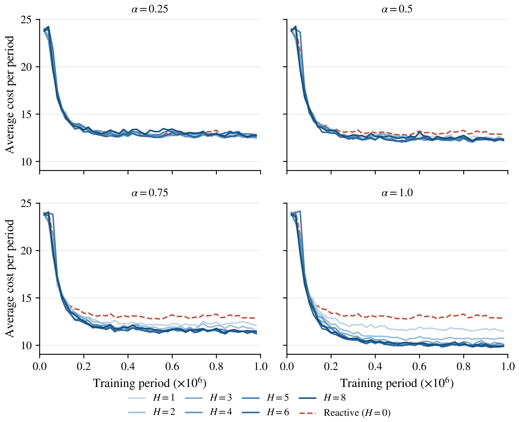
All configurations are trained for the same run length of ${10}^6$ periods, sufficient for even the rarest disruption grade to occur roughly $2.5\times {10}^4$ times. Training curves for all configurations have flattened by the end of the run, as reported in Appendix A.

6.2. Compared Policies and Performance Metrics

Three policies are compared. The first is the calibrated (s, Q) policy, which uses only the inventory position. The second is a reactive deep reinforcement learning policy, trained on the state of Equation (5) in Section 4.3 without the predicted sequences. It observes the internal variables and the current disruption status but receives no advance information. The third is the proposed risk sensing policy, trained on the full state of Equation (5). The two DRL policies share the same architecture, hyperparameters, and training procedure of Section 5 and differ only in the state, so the performance gap between them isolates the value of the precursor signal.

The static benchmark is a periodic review (s, Q) policy with a review interval of one period, which places an order of size Q whenever $\mathit{IP}\left(t\right)\le s$ at a review epoch. Under the shared action space, the order is restricted to a single lot per period; the standard (s, nQ) variant, which orders as many lots as needed to raise the inventory position above s, lies outside this action space and is discussed in Section 8. To make the benchmark as strong as possible, the reorder point is calibrated by grid search on the same environment including disruptions, selecting the integer s that minimizes the long-run average cost. The calibration uses a sample path separate from the evaluation runs, so the benchmark is not tuned on the evaluation data. The calibration is repeated for every environment variation considered, so the benchmark faces each condition with its own best reorder point. The calibrated values are reported with the results in Section 7. All policies, including the benchmark, operate under the same action space, placing at most one lot per period.

In addition to these three policies, we evaluate a signal-triggered heuristic, a transparent rule that reads the same signal as the risk sensing policy and operates the same action space but replaces the learned mapping with a signal-dependent reorder point applied to the inventory position. In calm conditions the rule orders whenever the inventory position falls to a base reorder point or below; when a disruption is predicted to be active within the next w periods, the reorder point is raised by a grade-specific increment. The five parameters (the base reorder point, three increments, and the window w) are calibrated by coordinate search on the same calibration sample path used for the static benchmark’s s, scanning each parameter in turn over its range and iterating until no further improvement. The purpose of this rule is to separate the value of the information from the contribution of learning (Section 7.1).

Each configuration is trained ten times, with independent random seeds governing the network initialization, the exploration sampling, and the training period realizations. Each trained policy is evaluated over $2\times {10}^5$ periods on ten evaluation runs, each using an independent realization of demand and disruptions generated from seeds distinct from those used in training. These evaluation seeds are shared across all policies and configurations, so that differences reflect the policies rather than sampling variation. For the DRL policies, costs achieved on the evaluation runs are first averaged for each training seed. Results are then reported as means over the ten training seeds with 95% confidence intervals. For the (s, Q) benchmark, which has no training seeds, means and intervals are calculated directly over the ten evaluation runs. We report the long-run average cost per period together with its holding and shortage components. As a service measure, we also report the fill rate, the fraction of demand met immediately from on-hand stock.

Two sources of variation enter these results. The training seed changes the learned policy itself, and the evaluation stream changes the sample path on which a policy is tested. Because the ten evaluation streams are shared by all policies and configurations, differences between policies are not driven by which test streams were sampled but by the training seed under which the policy was trained. The confidence intervals for the DRL policies capture this variation across the training seeds.

Comparisons are paired wherever two policies share the same random realizations. The two DRL policies (reactive and risk sensing) share training seeds and evaluation streams, and their comparison is a paired t-test by training seed, each summarized by its mean over the ten evaluation streams. At quality $\alpha <1$ the signal itself is also random in which disruptions it detects, and each training seed of the risk sensing policy observes its own signal realization, with the heuristic evaluated under the same ten realizations on the same streams. Their comparison is therefore also a paired t-test, by signal realization, summarized in the same way. The calibrated benchmark has neither training seeds nor signal realizations. Its comparison with a DRL policy is therefore a one-sample t-test of the ten training seed means against the benchmark mean, where both means are computed on the same ten evaluation streams, so the comparison is not affected by stream-sampling noise.

For the DRL policies we also probe the trained network directly. The policy is queried across inventory levels in a state with an empty pipeline, where inventory level and inventory position coincide, and with no active disruption. The highest inventory level at which the policy places an order is termed the effective reorder point, which makes the otherwise black-box ordering rule visible and directly comparable with the static benchmark’s s. When the signal inputs additionally predict no upcoming disruption, the probed state is one in which no disruption is active and none is expected, which we call the calm state. The corresponding threshold, the calm-state reorder point, is reported alongside the main results. Section 7.3 queries the policy in the same way, with a predicted disruption entered in the signal inputs, tracing how the reorder point rises with the severity and proximity of the threat.

7. Results

7.1. Overall Comparison

Table 5. Average cost per period of the three policies: the calibrated (s, Q) policy, the reactive policy, and the risk sensing policy over the full grid of predictive horizons H and signal qualities $\alpha$. Means with 95% confidence intervals over the ten training seeds; for the (s, Q) benchmark, over the ten evaluation streams. Bold: significantly below the (s, Q) benchmark ($p<0.05$, one-sample t-test over the ten training seeds against the benchmark mean).

Policy	Signal Quality
	$\mathit{\alpha }=\mathbf{0.25}$	$\mathit{\alpha }=\mathbf{0.5}$	$\mathit{\alpha }=\mathbf{0.75}$	$\mathit{\alpha }=\mathbf{1.0}$
(s, Q)	12.18 ± 0.06
Reactive ($H=0$)	12.57 ± 0.15
Risk sensing, $H=1$	12.35 ± 0.16	12.12 ± 0.16	11.95 ± 0.21	11.34 ± 0.14
$H=2$	12.46 ± 0.29	12.13 ± 0.17	11.62 ± 0.38	10.49 ± 0.33
$H=3$	12.28 ± 0.19	12.00 ± 0.30	11.20 ± 0.20	9.97 ± 0.19
$H=4$	12.35 ± 0.31	11.95 ± 0.23	11.10 ± 0.07	9.68 ± 0.19
$H=5$	12.47 ± 0.22	11.82 ± 0.14	11.10 ± 0.11	9.50 ± 0.07
$H=6$	12.42 ± 0.30	11.93 ± 0.21	11.05 ± 0.07	9.49 ± 0.06
$H=8$	12.48 ± 0.14	12.16 ± 0.37	11.19 ± 0.17	9.52 ± 0.09
Best cell vs. (s, Q) benchmark	$+0.8\%$	$-2.9\%$	$-9.3\%$	$-22.0\%$

Under Benjamini–Hochberg false discovery rate control at the 0.05 level across the 28 risk sensing cells, the bold set is unchanged except that $H=1$, $\alpha =0.75$ becomes marginal (adjusted $p=0.051$).

reports the average cost of the two benchmark policies and of the risk sensing policy over the full grid of predictive horizons and signal qualities. The first is the calibrated (s, Q) policy, the static rule without advance information, whose grid-searched reorder point yields an average cost of 12.18 ± 0.06. The second is the reactive policy, trained identically to the risk sensing policy but without the precursor signals, which reaches 12.57 ± 0.15, significantly worse than the (s, Q) policy. Although the state of the reactive policy is a superset of the (s, Q) policy’s single input, the inventory position, the learned policy does not match the exhaustively calibrated static rule, which is consistent with earlier observations that DRL does not outperform well-tuned policies in structured settings [4,14]. In this environment, deep reinforcement learning by itself does not produce a gain. Any gains must therefore come from the information exploited.

The table shows that at $\alpha =0.25$ every horizon stays above the static (s, Q) benchmark, and at $\alpha =0.5$ the policy achieves at most a marginal gain. Only when $\alpha \ge 0.75$ does advance information yield a substantial gain, lowering the cost significantly below the static benchmark at every horizon and by up to 22.0% at the grid minimum. As with the learning method, information by itself does not produce a gain. It becomes valuable only when the signal is reliable enough to act on. How the gain depends on the predictive horizon and the signal quality is analyzed in Section 7.2.

Table 6. Performance of the compared policies at the reference configuration ($H=6$, $\alpha =0.75$). Means over the ten training seeds with 95% confidence intervals; for the (s, Q) benchmark, mean and interval over the ten evaluation streams; for the signal-triggered heuristic (Section 6.2), over ten signal realizations. The effective reorder point is reported as the modal value across training seeds; for the heuristic it is the calibrated calm-state reorder point.

Policy	Avg. Cost	Holding	Shortage	Fill Rate (%)	Effective Reorder Point
(s, Q)	12.18 ± 0.06	10.99 ± 0.00	1.19 ± 0.06	98.5 ± 0.0	9
Reactive	12.57 ± 0.15	9.82 ± 0.27	2.75 ± 0.40	97.1 ± 0.4	8
Signal-triggered heuristic	11.24 ± 0.01	9.82 ± 0.00	1.42 ± 0.01	98.1 ± 0.0	7
Risk sensing	11.05 ± 0.07	9.19 ± 0.28	1.86 ± 0.28	97.6 ± 0.4	6

details the comparison at $H=6$, $\alpha =0.75$, chosen as the reference configuration on which the analysis of the policy’s operating mechanism and the sensitivity analysis in subsequent sections are based. At this configuration the predictive horizon covers three quarters of the longest delivery cycle, and the signal detects three quarters of upcoming disruptions, so the advance information is useful but imperfect. Compared to the benchmark policies, the risk sensing policy lowers the average cost to 11.05 ± 0.07, a reduction of 9.3% against the static (s, Q) policy and 12.1% against the reactive policy. The latter gap, between two identically trained policies that differ only in the signal, isolates the value of the precursor signal. This shows that even imperfect advance information can deliver substantial cost savings.

The calibrated (s, Q) benchmark attains an average cost of 12.18, composed mostly of holding cost (10.99). This indicates that, with $s=9$, the policy tends to maintain a large inventory buffer against disruptions that rarely occur. The learned calm-state reorder point of the risk sensing policy is 6 (the modal value across training seeds), well below the calibrated static reorder point, and rises only when a warning arrives (Section 7.3). Rather than paying for a large buffer, the risk sensing policy substitutes information for inventory, holding less stock in calm periods and rebuilding it selectively ahead of predicted disruptions, in line with the classical result that advance information can replace safety stock [20]. The policy’s fill rate is slightly below the static benchmark’s (97.6% vs. 98.5%), with a correspondingly higher shortage cost. The value of advance information might be expected to come from the protective stock accumulated ahead of disruptions, but most of the gain over the static benchmark comes instead from avoiding the cost of a large buffer stock held as insurance in calm periods. How the policy produces these savings is systematically examined in Section 7.3.

The comparison above leaves open how much of the risk sensing policy’s gain requires learning at all, rather than the signal itself. To separate the two, we evaluate the signal-triggered heuristic of Section 6.2. The calibrated rule raises the reorder point from a base of 7 to 10 when a grade-1 disruption is predicted within two periods, by two units for a grade-2 disruption, and not at all for a grade-3 disruption.

Evaluated under the protocol of Section 6.2 (ten signal realizations on the ten evaluation streams), the heuristic attains 11.24 ± 0.01, between the static benchmark (12.18) and the risk sensing policy (11.05). A transparent rule with five parameters thus captures about 83% of the total gain (0.94 of 1.13 cost units), confirming that most of the value comes from the information itself. The remaining 17% is contributed by learning: the risk sensing policy improves on the heuristic by 0.19 (paired $t\left(9\right)=6.2$, $p<0.001$ over the shared signal realizations), operating a leaner calm state (calm-state reorder point 6 versus the heuristic’s 7) with lower holding cost overall (9.19 vs. 9.82 per period) and a finer escalation than the fixed rule expresses. The heuristic conditions only on the aggregate inventory position and the nearest predicted disruption, whereas the learned policy maps the full state, including the composition of the pipeline and the complete predicted sequences, and is not restricted to a threshold form. Notably, the calibrated rule reproduces the response structure extracted from the learned policy in Section 7.3—a strong response to grade-1 warnings, a mild one to grade-2, and none to grade-3—although the two were obtained independently.

7.2. Effect of the Predictive Horizon and Signal Quality

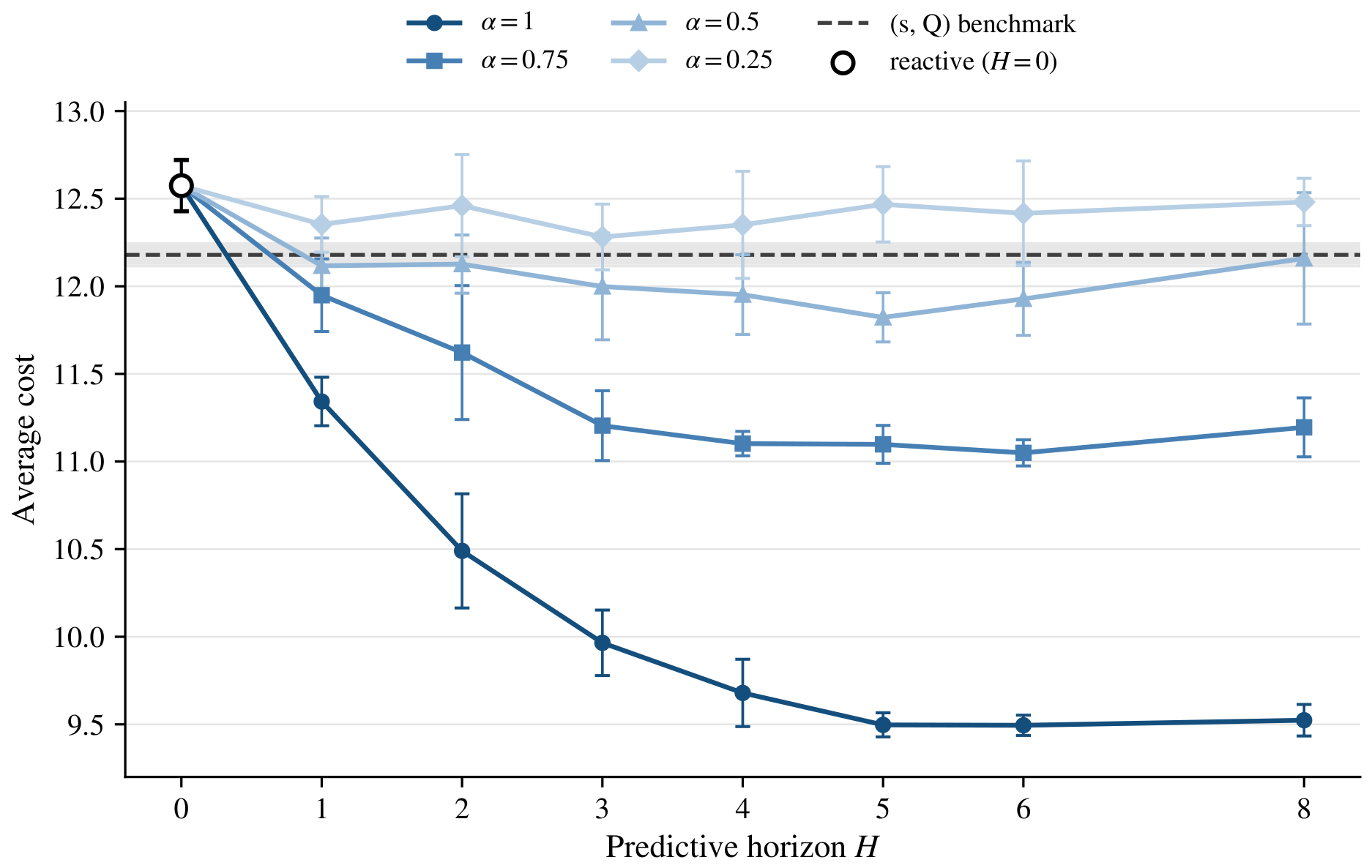
Figure 1 plots the grid of Table 5 as the average cost against the predictive horizon, one curve per signal quality, with the reactive policy at $H=0$ as the common origin and the calibrated benchmark as a horizontal reference. The curves divide into three regimes along the signal quality axis. For reliable signals ($\alpha \ge 0.75$), even a one-period horizon yields a gain over the benchmark policies. A single period of warning is enough to bring an order forward, if needed, ahead of the disruption onset, and that order can still be delivered at the normal lead time. The cost falls steeply as the horizon grows, since at most one lot can be ordered per period and additional periods of warning therefore allow additional lots to be secured in advance. At $\alpha =1$, the successive gains from one more period of horizon are 1.23, 0.85, 0.52, 0.29, and 0.18 up to $H=5$, and essentially zero from $H=5$ to $H=6$. The intermediate quality $\alpha =0.5$ falls slightly below the static benchmark at intermediate horizons (11.82–12.00 across $H=3$–6, vs. 12.18 for the (s, Q) benchmark). This gain, however, is marginal, at most about three percent, and reaches statistical significance only at $H=5$ and $H=6$ ($p<0.001$ and $p=0.02$ over the training seeds). Although it does not fall behind the static benchmark, a signal that detects only half of upcoming disruptions offers little improvement over a well-calibrated static rule. For weak signals ($\alpha =0.25$) no horizon helps (12.28–12.48). Improving on a calibrated static rule therefore requires not the mere presence of advance information but sufficient reliability. The break-even quality lies between $\alpha =0.25$ and $\alpha =0.5$ in this environment.

Beyond $H=4$ the improvement becomes marginal. The reason is structural, as a horizon of a few periods is sufficient to act on a warning in the environment studied. Protecting against the most severe disruption means covering ${\Delta }_{\max }=6$ additional periods of demand on top of the normal lead time, which corresponds to an additional stock of 7–8 units above the calm state at the service level implied by the shortage cost. Since each period of ordering adds only about two units of net stock ($Q-\lambda =2$), the buildup takes about four periods. Look-ahead beyond this span therefore adds little value, and we call this span the effective horizon. Its length is a property of the action space, not of the signal. An action space permitting larger orders per period would complete the buildup sooner and shorten the effective horizon accordingly.

The outcome is a plateau. At $\alpha =0.75$ the cost is 11.10, 11.10, 11.05, and 11.19 at $H=4$, 5, 6, and 8, with no significant seed-paired difference among the four (the largest, $H=8$ vs. $H=6$, is $+0.15$, $t\left(9\right)=1.62$, $p=0.14$), and the pattern at $\alpha =1$ is the same (9.68, 9.50, 9.49, 9.52). Since a longer horizon strictly enlarges the information set, the value of the optimal policy is non-decreasing in H. What happens beyond the effective horizon is therefore primarily a property of learning. The additional state dimensions have no measurable effect, as learning neither extracts further value from them nor degrades in their presence. Although we noted in Section 4.2 that the burden of learning in an enlarged state space might offset the richer information of a longer horizon, no such effect is detected within the tested range, as all horizons at or beyond the effective horizon perform alike. To rule out the possibility that the plateau reflects limitations of the learning setup rather than the effective horizon itself, we retrained the $\alpha =0.75$ cells at $H\in \{4,6,8\}$ with twice the training run length and, separately, with the actor and critic widened to $2\times 64$ units. Under both variants the three horizons continue to perform alike, with no consistent ordering (Appendix B).

How early a warning arrives depends on the pace at which the disruption develops and is discovered [26,33] and on the warning capability of the firm [34]. The model studied here fixes the lead of every detected disruption at H and therefore does not represent the pace of disruption. The results along the horizon axis nevertheless suggest what its effect would be. A gradually developing disruption, such as mounting port congestion or an escalating labor dispute, would be recognized several periods ahead and corresponds to the right end of Figure 1, where the gain is complete. A disruption that develops suddenly, by contrast, might become recognizable only a few periods before its onset. When such a late warning appeared, the policy would bring its orders forward as it has learned, but the periods that had already passed without a warning could not be recovered, and the stock that would have been accumulated in them would be missing. The effect would resemble that of a shorter horizon in Figure 1, where the gain of the policy diminishes as the horizon shrinks. A disruption that gives no usable warning at all, such as a fire or an earthquake, is observed only at its onset and handled reactively, which the model does represent through the undetected fraction. In these terms, disruptions with no warning lower the detection rate and disruptions with late warnings shorten the horizon, so that the pace of disruption would enter the results through the two parameters that the experiments vary. The effect of a varying pace of disruption, and of the mix of leads it produces, is not quantified in this study. This limitation is stated in Section 8.

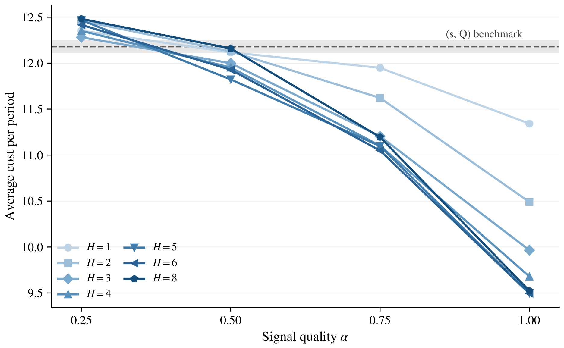
Figure 2 shows how the average cost changes with the signal quality at each horizon. The cost decreases in $\alpha$ at every horizon, and the decrease steepens with H. At $H=1$, moving from $\alpha =0.25$ to $\alpha =1$ lowers the cost by about 8%, while at $H=4$ or beyond the same movement saves 22–24%. Quality and horizon are thus complementary. A long horizon raises the value of a reliable signal, and a reliable signal is required for a long horizon to be useful. The marginal return also grows with quality. At every horizon $H\ge 2$, the step from $\alpha =0.75$ to $\alpha =1$ yields a larger saving than the step from $\alpha =0.25$ to $\alpha =0.5$ (e.g., 1.55 vs. 0.49 at $H=6$). Unlike the earlier steps, which only reduce the remaining uncertainty, the step to full quality removes the uncertainty entirely, yielding the largest improvement.

7.3. Operating Mechanism of the Learned Policy

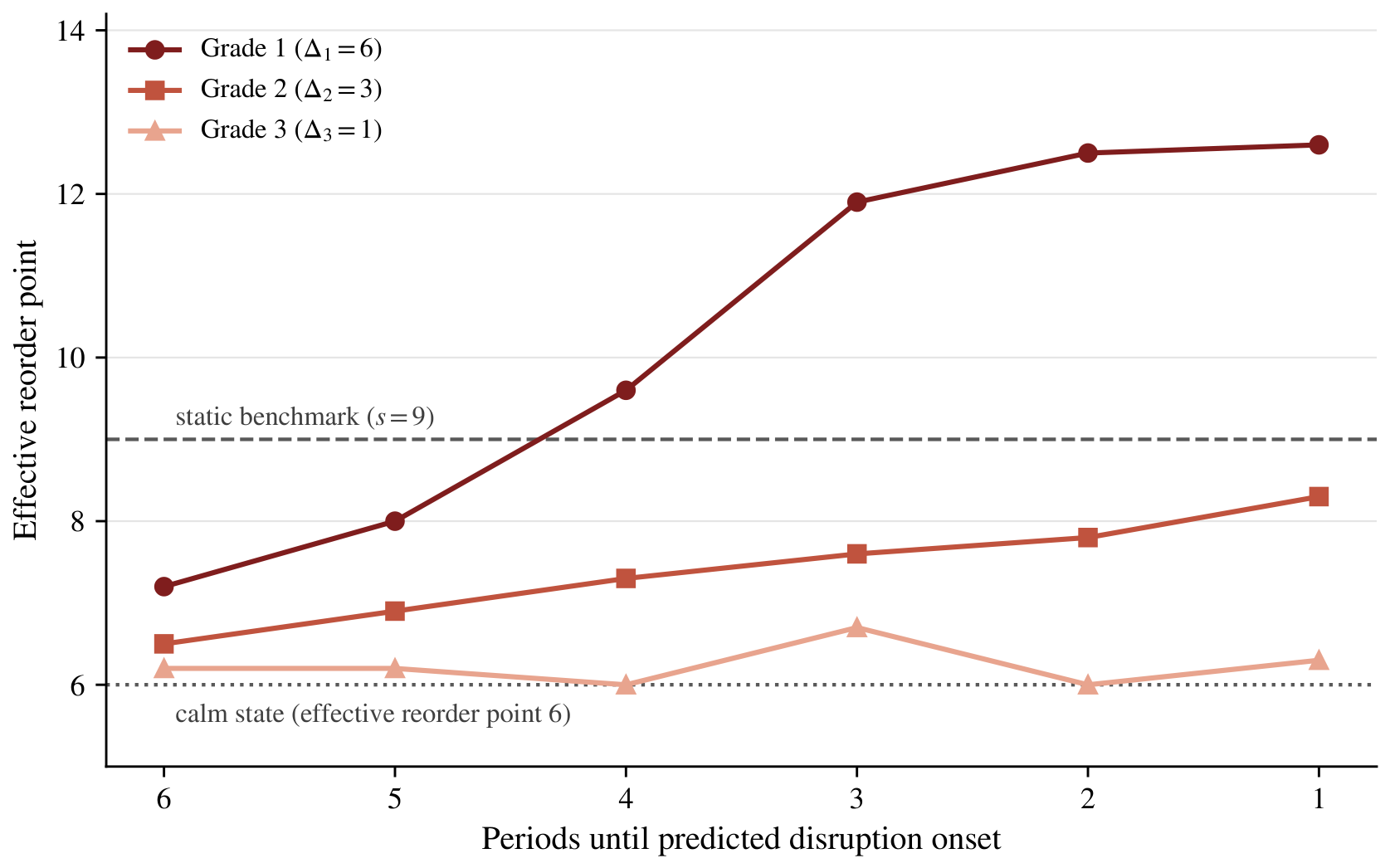
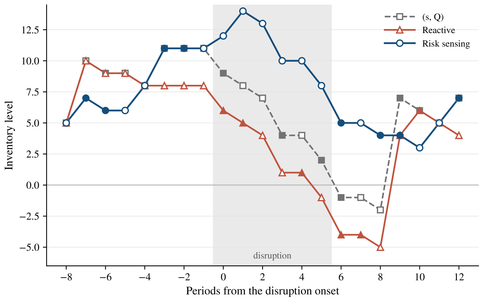
Figure 3 reports the effective reorder point of the risk sensing policy as a function of the warning state, that is, the severity grade of the predicted disruption and the number of periods until its onset. Under a grade-1 warning (${\Delta }_1=6$) the effective reorder point rises from the calm-state value of 6.0 to 12.6 as the onset approaches, exceeding the static $s=9$ about four periods in advance. A grade-2 warning (${\Delta }_2=3$) induces a mild rise to about 8, and a grade-3 warning (${\Delta }_3=1$) induces essentially no response, which is reasonable since a one-period delay is absorbed by the calm-state buffer. The policy thus operates a state-dependent reorder point that rises with the severity and proximity of the predicted threat, which is the feedforward mechanism anticipated in Section 4.3. The rise is visible as soon as a grade-1 warning enters the horizon (7.2 at six periods before the disruption onset, versus 6.0 in the calm state) but remains modest until about five periods before the onset, then steepens sharply over the final four periods, which correspond to the effective horizon identified in Section 7.2. Starting the buildup too early would incur unnecessary holding cost, while starting it late would leave too few ordering periods to complete it. The pre-positioning is thus concentrated where it is needed. The probe characterizes the policy on a selected slice of the state space, with an empty pipeline and a single predicted event, so it visualizes the response structure rather than describing the policy exhaustively. The same mechanism is visible in the trajectory of Figure 4 and the decomposition of

Table 7. Average cost per period of the three policies in the calm and the exposed periods (37% and 63% of all periods, respectively) at the reference configuration ($H=6$, $\alpha =0.75$). Means over the ten training seeds with 95% confidence intervals; for the (s, Q) benchmark, over the ten evaluation streams.

Policy	Calm Periods			Exposed Periods
	Avg. Cost	Holding	Shortage	Avg. Cost	Holding	Shortage
(s, Q)	10.98 ± 0.00	10.97 ± 0.00	0.00 ± 0.00	12.88 ± 0.10	10.99 ± 0.00	1.89 ± 0.10
Reactive	9.79 ± 0.36	9.78 ± 0.37	0.01 ± 0.00	14.19 ± 0.42	9.84 ± 0.25	4.35 ± 0.64
Risk sensing	8.96 ± 0.30	8.90 ± 0.32	0.07 ± 0.03	12.26 ± 0.18	9.36 ± 0.26	2.90 ± 0.42

, both obtained from the evaluation runs without any such restriction.

Figure 4 shows the inventory level of the three policies around an illustrative grade-1 disruption, on the evaluation stream common to the three policies. Ahead of the disruption onset, only the risk sensing policy builds up stock. When the disruption begins, it holds about two additional lots relative to its calm level, the buildup quantified in Section 7.2, while the (s, Q) and reactive policies remain at their calm-state inventory levels. During the six disrupted periods all three policies consume their stock, but the risk sensing policy does so from the pre-positioned level and remains positive throughout, whereas the two benchmark policies suffer backorders near and after the end of the disruption. Moreover, the (s, Q) and reactive policies keep placing orders during the disruption, and these orders cannot be delivered until the disruption ends, resulting in backorders that persist until the delayed lots finally arrive and restore their inventory levels.

Aggregating over the full evaluation horizon, the advantage of the risk sensing policy over the reactive policy extends to both cost components (holding 9.19 vs. 9.82, shortage 1.86 vs. 2.75; see Table 6). To identify where these gains arise, we split the evaluation horizon into two parts. One part comprises the exposed periods, during which the system remains under the influence of a disruption, from the disruption onset until the last delayed delivery can arrive ($\tau$ periods after normal supply resumes). The other comprises the calm periods, the remaining periods free from the influence of any disruption. The two parts account for 63% and 37% of all periods, respectively. Table 7 reports the cost of each policy in the two parts, with its holding and shortage components. We find that the saving of the risk sensing policy over the static (s, Q) policy comes primarily from the calm periods (8.96 vs. 10.98 per period), almost entirely in holding cost. This difference is due to the buffer stock held as insurance, of which the risk sensing policy holds substantially less, as anticipated in Section 7.1. In contrast, the saving over the reactive policy comes from the exposed periods (12.26 vs. 14.19 per period), mostly in shortage cost, due to the stock positioned upon a warning before lead times lengthen. Together, the two comparisons show that the precursor signal lets the policy hold less stock in calm periods and more stock ahead of predicted disruptions.

7.4. Sensitivity to the Environment

Table 8. Reference configuration comparison under environment variations ($H=6$, $\alpha =0.75$; means over the ten training seeds with 95% confidence intervals, and over the ten evaluation streams for the recalibrated (s, Q) benchmark). s recalibrated per environment; the signal value is the reactive minus the risk sensing cost, with mean and 95% confidence interval over the seed-paired differences.

Environment	s	(s, Q)	Reactive	Risk Sensing	Signal Value
Base ($p=100$)	9	12.18 ± 0.06	12.57 ± 0.15	11.05 ± 0.07	1.52 ± 0.16
$p=50$	7	11.00 ± 0.05	11.21 ± 0.11	9.96 ± 0.18	1.26 ± 0.26
$p=200$	10	13.20 ± 0.10	13.93 ± 0.50	12.51 ± 0.38	1.42 ± 0.45
Disruptions $\times 0.5$	7	11.03 ± 0.07	11.41 ± 0.15	9.70 ± 0.09	1.71 ± 0.12
Disruptions $\times 2$	10	13.18 ± 0.07	13.71 ± 0.28	12.76 ± 0.21	0.95 ± 0.26

repeats the reference-configuration comparison under four variations of the environment: shortage cost $p\in \{50,200\}$ and disruption frequencies scaled by $0.5$ and 2. The (s, Q) benchmark is recalibrated for each environment. The value of the precursor signal, defined as the gap between the reactive and risk sensing policies, persists across all variations, ranging from 7% to 15% of the reactive policy’s cost, and the risk sensing policy remains superior to the recalibrated (s, Q) benchmark in every environment.

The size of the risk sensing policy’s advantage, however, depends on the disruption frequency. With rare disruptions ($\times 0.5$) the advantage over the recalibrated (s, Q) benchmark is largest (9.70 vs. 11.03, a 12% reduction, and the tightest confidence interval in the table), and the signal value reaches its maximum of 1.71 (9.70 vs. 11.41, a 15% reduction). When shocks are infrequent, a static buffer sized for them is idle most of the time, so replacing it with information-triggered accumulation is most profitable. With frequent disruptions ($\times 2$) the cost gaps narrow to their minimum. The advantage over the recalibrated (s, Q) benchmark falls to about 3% (12.76 ± 0.21 vs. 13.18 ± 0.07), though it remains clearly significant. The (s, Q) benchmark raises its reorder point to $s=10$, and its permanent buffer, idle under rare shocks, is well utilized under near-continuous ones, so there is less insurance cost for the risk sensing policy to avoid. The signal value also shrinks to 0.95 (12.76 vs. 13.71, a 7% reduction). More frequent warnings arrive while the system is still recovering from an earlier disruption, and since building up inventory takes time, less of each warning can be converted into protective stock.

In contrast, varying the shortage penalty has no systematic effect on the signal value (1.26, 1.52, and 1.42 at $p=50$, 100, and 200). The variation is not monotonic in p, and given the seed-level variability, the differences are not statistically significant (analysis of variance with the training seed as a blocking factor, $F(2,18)=1.40$, $p=0.27$).

The value of the precursor signal therefore depends on how often disruptions occur, while no dependence on the shortage cost is detected within the tested fourfold range. Precursor signals are most valuable where static policies are weakest, in environments where severe disruptions are infrequent, so that a permanent buffer is wasteful and timely anticipation can replace it. The frequency axis is varied directly in these experiments, while the severity profile is held fixed. The role of severity is instead visible in the policy’s responses to the different grades, where it responds strongly to the severe grade and not to the mild one (Section 7.3).

8. Discussion

The main finding of this study is that a precursor risk signal has substantial value in inventory control, but only under certain conditions. Incorporating the signal into the state of a PPO agent reduced the average cost by 9.3% against a calibrated (s, Q) policy and by 12.1% against an identically trained reactive policy at the reference configuration, and the advantage over the recalibrated (s, Q) policy persisted across every environment variation. The decomposition of Section 7.3 identifies where the gains arise. Against the static (s, Q) policy, the saving arises in the calm periods, where the policy holds substantially less of the insurance buffer. Against the reactive policy, the saving arises in the exposed periods, where stock positioned upon a warning prevents shortages. The signal thus lets the policy substitute information for inventory, holding less stock in calm periods and more stock ahead of predicted disruptions. This extends the classical demand-side result of Hariharan and Zipkin [20] to supply-side advance information in a learning setting.

Three aspects of the results have practical implications. First, the horizon response shows a plateau rather than an interior optimum. Once the effective horizon is covered, that is, the few ordering periods needed to accumulate protective stock (about four here, under the one-lot-per-period action space), additional look-ahead brings neither measurable cost nor benefit. The plateau persists even when the training run length is doubled and the neural networks are widened. For practice, this makes horizon selection forgiving. A forecast need not reach far into the future to be useful and providing a longer horizon than necessary does no harm within the tested range.

Second, the critical requirement is signal quality. Advance information is valuable only above a reliability threshold. A signal that detects half of upcoming disruptions offers only a marginal gain over a well-calibrated static rule, and a weaker one falls behind it. Investments in sensing infrastructure should therefore be judged by the detection rate they can deliver, not by the length of the forecast horizon.

Third, the value of the signal depends on the disruption frequency, while no dependence on the shortage penalty was detected within the tested range. The value is largest where severe disruptions are rare, because a static buffer held against them is idle most of the time. The value decreases considerably where disruptions are frequent, because the buffer is then in regular use and warnings arrive faster than stock can be accumulated. Precursor signals are therefore most useful in environments with low-probability, high-impact disruptions.

The leading indicators of Table 1 are observable but reading them as a warning that a disruption is coming is a judgment, and that judgment is a matter of perception. Managers’ perception of supply risk is subjective, and their actions follow their perception [35], and indicators that look clear in hindsight are often ambiguous beforehand. Instead of representing this judgment, the model relies on what the indicators and the judgment together leave behind. Looking back over a period, one can count how many disruptions were recognized before they began and how many periods in advance, and these two quantities are the detection rate and the predictive horizon. They are properties of a firm’s monitoring that are established in hindsight, not quantities known in advance. As noted in Section 3, the practice from which the problem is abstracted tracks both quantities. The model takes them as given, and the policy is learned for a given detection rate and horizon, so that it prescribes how to act on a signal of that quality, whose value is then measured in the experiments (Section 7.2).

Acting on advance information before a disruption arrives is also the purpose of scenario planning [36], a managerial practice with a long history, and the two approaches can be used in a complementary way. Developed at Royal Dutch/Shell in the 1970s [37], scenario planning constructs multiple internally consistent scenarios of how the business environment could unfold, uses them to help managers reperceive their exposure, and selects the leading indicators that would show which scenario is unfolding [38]. Its application to supply chains and logistics has been developed in later studies [39,40,41]. Scenario planning identifies the strategic options each scenario calls for, and the model studied here can be applied based on that selection at the operational level. In the terms of Section 3, each scenario corresponds to a disruption type in Table 1, with its grade and the indicators that precede it. For each such scenario, the model derives the ordering response, as a learned policy or as the transparent rule of Section 6.2, and quantifies its expected cost and service level under the detection rate and horizon achievable with the selected indicators. The results then return to the scenario stage. They show which scenarios are worth monitoring and how reliable their indicators must be. In this study, that threshold is found to be a detection rate above one half. The two tools thus form a loop rather than a sequence.

A drawback of a DRL policy is its lack of transparency, which scenario planning provides through scenarios and indicators that a manager can follow. A rule can be considered in place of the DRL policy to address this. In this study, the signal-triggered heuristic, which reads the same signal through five interpretable parameters, retains about 83% of the measured benefit, indicating that most of the value comes from the information itself rather than from the learning method. A manager who requires a transparent instrument can adopt the rule, and the additional value of the less transparent DRL policy becomes a quantified increment rather than an assumption.

For a manager considering adoption, the results suggest the following steps. First, classify the firm’s exposure by the disruption types of Table 1 and identify the indicators available for each, which is the task that scenario planning supports. Second, estimate the detection rate and the horizon of the current monitoring from past disruptions, as the practice studied does (Section 3). Third, if the detection rate exceeds about one half, act on the signal, initially through the transparent rule of Section 6.2, which requires only a base reorder point and grade-specific increments and captures most of the gain, and through a learned policy where the remaining gain justifies it. Fourth, evaluate investments in monitoring by the detection rate they add rather than by the horizon they extend, since the value of the signal saturates beyond a few periods of warning but rises steeply with the detection rate. The saving to expect relative to a well-calibrated static rule depends on the disruption frequency, from about 3% where severe disruptions are frequent to about 12% where they are rare (Section 7.4).

Several limitations should be noted. The model contains a single response lever, the timing of replenishment orders. In practice, disruption types differ in the responses they call for, such as rerouting or expediting for a transport disruption, a second source for a supplier outage, or product substitution for a discontinued component. Earlier ordering was chosen because it is available for every disruption type and requires no contractual or design change, and fixing the lever isolates the value of the information from the value of the means to act on it. Additional levers would give a signal-aware policy more ways to convert a warning into protection, but a static policy would gain the same levers, so their net effect on the value of the signal cannot be determined without modeling them. The results should therefore be read as the value of advance information when the only available response is to reorder earlier, which is the response common to all disruption types.

The action space permits at most one lot per period, which limits the rate at which a warning can be converted into protective inventory. An action space allowing multiples of the lot size (an (s, nQ)-type policy) would speed up this conversion, shortening the effective horizon of Section 7.2, and could change the measured value of the signal in either direction, since faster accumulation benefits the signal-based policies and the benchmark alike.

The model also assumes that the supplier keeps accepting orders during a disruption. Where a disruption removes the supplier’s capacity so that orders are rejected, the manufacturer cannot replenish at all until recovery, and protective inventory built before the onset becomes the only source of supply for the duration. For disruptions short enough to be covered by pre-positioned stock, the value of a warning would then be larger than measured here, since pre-positioning is the sole response available, whereas for longer ones both the signal-based and the static policies run out of stock and the gap narrows. The value of a warning under rejected orders thus depends on the length of the disruption relative to the stock that can be pre-positioned, and establishing this dependence requires modeling the rejection explicitly, which is a direction for extension.

The signal model is stylized. It models missed detections, with probability $1-\alpha$, but not false alarms, and a detected disruption carries its true severity and timing, whereas real leading indicators also produce false positives and imprecise estimates. The warning lead is also constant, fixed at H for every detected disruption, whereas real disruptions differ in the pace at which they develop and become recognizable. A false alarm would trigger a protective buildup for a disruption that never arrives, and its cost is the temporary holding of unneeded stock, whereas a missed detection exposes the system to the full shortage cascade of an unanticipated disruption. Under the cost structure studied here, false alarms are therefore expected to erode the value of the signal gradually rather than eliminate it, but quantifying this erosion, and the false-alarm rate at which a signal stops being worth acting on, requires extending the signal model and is left for future work.

Demand is stationary, the system is a single-item, two-echelon chain, and only the inbound supply process is modeled, so disruptions to the manufacturer’s outbound logistics lie outside the scope of the model. Section 3 relates this restriction to the disruptions that affect both sides. When both sides are disrupted, the manufacturer must decide whether to reduce production while shipments are blocked and components are themselves in short supply, and whether to adjust its component inventory accordingly. An outbound warning may thus call for the opposite of what an inbound warning calls for, and a planner who receives both must weigh them together. Extensions to outbound disruptions, interactions between demand-side and supply-side information, and the propagation of warnings through deeper supplier networks are left for future research.

Finally, although disruptions produce structural breaks in realized lead times, the underlying risk profile is fixed over time, so the environment is stationary in the stochastic process sense and the risk profile can be learned. Genuine non-stationarity, that is, structural change in the risk profile itself, would require online adaptation beyond the scope of this paper.

9. Conclusions

This paper developed a risk sensing deep reinforcement learning framework for inventory control under supply disruptions. The state of a PPO agent is augmented with precursor risk signals, which predict the severity and timing of upcoming disruptions, so that the replenishment decision acquires a feedforward component. The learned policy operates a state-dependent reorder point that stays low in calm conditions and rises with the severity and proximity of a predicted threat, positioning protective inventory before lead times lengthen rather than after.

Treating signal quality and predictive horizon as explicit design parameters allowed the value of advance information to be measured directly. The risk sensing policy outperforms both a per-environment calibrated (s, Q) policy and an identically trained reactive policy whenever the signal is sufficiently reliable, and the comparison with the reactive policy isolates the value of the signal itself (RQ1). That value requires only a short horizon, enough to complete the protective buildup, but it does require a sufficiently high detection rate (RQ2). The value is greatest where severe disruptions are infrequent and static buffers are therefore most wasteful. In this environment, neither deep reinforcement learning by itself nor an unreliable signal produced a gain. A transparent signal-triggered rule captured about 83% of the gain, with learning contributing the rest (RQ3). The gains reported here come from reliable information, not from the learning method alone. The practical message for supply chain managers is that the transition from reactive response to proactive mitigation depends on sensing infrastructure. Even an imperfect early-warning capability can replace a substantial share of safety stock, provided that it detects a majority of upcoming disruptions a few periods in advance. These findings rest on a stylized simulation abstracted from a single industrial setting, and the quantitative magnitudes are specific to the environment studied. More general real-world settings remain to be addressed.

There are several directions for future research. On the modeling side, an action space that allows more than one lot per period and a signal model with false alarms, graded confidence, and warning leads that vary with the pace of the disruption would bring the setting closer to practice. Applying the combination of scenario planning and the model outlined in Section 8 to an actual firm would show how the disruption types and indicators selected at the scenario stage translate into the value of monitoring them. In multi-echelon systems, warnings could propagate across stages, and the questions become which tiers to monitor, how to integrate warnings that arrive from different tiers, and where in the chain protective stock should be positioned when a disruption is predicted upstream. Extending the action space with the type-specific responses of Table 1, such as expediting or a second source, would show how the value of a warning changes when more than one response is available. Finally, validation on empirical leading indicators, such as port-congestion indices or supplier risk alerts, would establish the detection rates and horizons that real signals deliver, the two parameters on which the value of the signal was shown to depend.

References

1. UN News. ‘No Precedent’ for Seafarers Caught in War Zone in Post-WW2 Era. Available online: https://news.un.org/en/story/2026/03/1167224 (accessed on 4 July 2026).
2. UNCTAD. Strait of Hormuz Disruptions: Implications for Global Trade and Development; UNCTAD/OSG/TT/INF/2026/1. Available online: https://unctad.org/publication/strait-hormuz-disruptions-implications-global-trade-and-development (accessed on 4 July 2026).
3. International Energy Agency. Oil Market Report—March 2026; IEA: Paris, France, 2026; Available online: https://www.iea.org/reports/oil-market-report-march-2026 (accessed on 30 July 2026).
4. Boute, R.N.; Gijsbrechts, J.; van Jaarsveld, W.; Vanvuchelen, N. Deep reinforcement learning for inventory control: A roadmap. Eur. J. Oper. Res. 2022, 298, 401–412. [Google Scholar] [CrossRef] [Scilit]
5. Madeka, D.; Torkkola, K.; Eisenach, C.; Luo, A.; Foster, D.; Kakade, S. Deep inventory management. arXiv 2022, arXiv:2210.03137. [Google Scholar] [CrossRef] [Scilit]
6. Alvo, M.; Russo, D.; Kanoria, Y.; Lee, M. Deep reinforcement learning for inventory networks: Toward reliable policy optimization. arXiv 2025, arXiv:2306.11246. [Google Scholar] [CrossRef] [Scilit]
7. Kaplan, R.S. A dynamic inventory model with stochastic lead times. Manag. Sci. 1970, 16, 491–507. [Google Scholar] [CrossRef] [Scilit]
8. Nahmias, S. Simple approximations for a variety of dynamic leadtime lost-sales inventory models. Oper. Res. 1979, 27, 904–924. [Google Scholar] [CrossRef] [Scilit]
9. Ehrhardt, R. (s, S) policies for a dynamic inventory model with stochastic lead times. Oper. Res. 1984, 32, 121–132. [Google Scholar] [CrossRef] [Scilit]
10. Zipkin, P. Stochastic leadtimes in continuous-time inventory models. Nav. Res. Logist. Q. 1986, 33, 763–774. [Google Scholar] [CrossRef] [Scilit]
11. Bradley, J.R.; Robinson, L.W. Improved base-stock approximations for independent stochastic lead times with order crossover. Manuf. Serv. Oper. Manag. 2005, 7, 319–329. [Google Scholar] [CrossRef] [Scilit]
12. Song, J.-S. The effect of leadtime uncertainty in a simple stochastic inventory model. Manag. Sci. 1994, 40, 603–613. [Google Scholar] [CrossRef] [Scilit]
13. Oroojlooyjadid, A.; Nazari, M.; Snyder, L.V.; Takáč, M. A deep Q-network for the beer game: Deep reinforcement learning for inventory optimization. Manuf. Serv. Oper. Manag. 2022, 24, 285–304. [Google Scholar] [CrossRef] [Scilit]
14. Gijsbrechts, J.; Boute, R.N.; Van Mieghem, J.A.; Zhang, D.J. Can deep reinforcement learning improve inventory management? Performance on lost sales, dual-sourcing, and multi-echelon problems. Manuf. Serv. Oper. Manag. 2022, 24, 1349–1368. [Google Scholar] [CrossRef] [Scilit]
15. van Hezewijk, L.; Dellaert, N.P.; van Jaarsveld, W.L. Scalable deep reinforcement learning in the non-stationary capacitated lot sizing problem. Int. J. Prod. Econ. 2025, 284, 109601. [Google Scholar] [CrossRef] [Scilit]
16. Dehaybe, H.; Catanzaro, D.; Chevalier, P. Deep reinforcement learning for inventory optimization with non-stationary uncertain demand. Eur. J. Oper. Res. 2024, 314, 433–445. [Google Scholar] [CrossRef] [Scilit]
17. Lu, X.; Wang, H.; Peng, Z.; Liao, C.; Liu, C. Dynamic optimization of multi-echelon supply chain inventory policies under disruptive scenarios: A deep reinforcement learning approach. Symmetry 2025, 17, 2078. [Google Scholar] [CrossRef] [Scilit]
18. Stranieri, F.; Stella, F.; Kouki, C. Performance of deep reinforcement learning algorithms in two-echelon inventory control systems. Int. J. Prod. Res. 2024, 62, 6211–6226. [Google Scholar] [CrossRef] [Scilit]
19. Temizöz, T.; Imdahl, C.; Dijkman, R.; Lamghari-Idrissi, D.; van Jaarsveld, W. Deep controlled learning for inventory control. Eur. J. Oper. Res. 2025, 324, 104–117. [Google Scholar] [CrossRef] [Scilit]
20. Hariharan, R.; Zipkin, P. Customer-order information, leadtimes, and inventories. Manag. Sci. 1995, 41, 1599–1607. [Google Scholar] [CrossRef] [Scilit]
21. Gallego, G.; Özer, Ö. Integrating replenishment decisions with advance demand information. Manag. Sci. 2001, 47, 1344–1360. [Google Scholar] [CrossRef] [Scilit]
22. Gavirneni, S.; Kapuscinski, R.; Tayur, S. Value of information in capacitated supply chains. Manag. Sci. 1999, 45, 16–24. [Google Scholar] [CrossRef] [Scilit]
23. Song, J.-S.; Zipkin, P. Inventory control with information about supply conditions. Manag. Sci. 1996, 42, 1409–1419. [Google Scholar] [CrossRef] [Scilit]
24. Ivanov, D. Supply chain viability and the COVID-19 pandemic: A conceptual and formal generalisation of four major adaptation strategies. Int. J. Prod. Res. 2021, 59, 3535–3552. [Google Scholar] [CrossRef] [Scilit]
25. Chopra, S.; Sodhi, M.S. Managing risk to avoid supply-chain breakdown. MIT Sloan Manag. Rev. 2004, 46, 53–61. [Google Scholar]
26. Sheffi, Y.; Rice, J.B., Jr. A supply chain view of the resilient enterprise. MIT Sloan Manag. Rev. 2005, 47, 41–48. [Google Scholar]
27. Tomlin, B. On the value of mitigation and contingency strategies for managing supply chain disruption risks. Manag. Sci. 2006, 52, 639–657. [Google Scholar] [CrossRef] [Scilit]
28. Tang, C.S. Robust strategies for mitigating supply chain disruptions. Int. J. Logist. Res. Appl. 2006, 9, 33–45. [Google Scholar] [CrossRef] [Scilit]
29. Žic, J.; Žic, S. Multi-criteria decision making in supply chain management based on inventory levels, environmental impact and costs. Adv. Prod. Eng. Manag. 2020, 15, 151–163. [Google Scholar] [CrossRef] [Scilit]
30. Schulman, J.; Wolski, F.; Dhariwal, P.; Radford, A.; Klimov, O. Proximal policy optimization algorithms. arXiv 2017, arXiv:1707.06347. [Google Scholar] [CrossRef] [Scilit]
31. Schulman, J.; Moritz, P.; Levine, S.; Jordan, M.; Abbeel, P. High-dimensional continuous control using generalized advantage estimation. In Proceedings of the International Conference on Learning Representations (ICLR), San Juan, Puerto Rico, 2–4 May 2016. [Google Scholar]
32. Dhariwal, P.; Hesse, C.; Klimov, O.; Nichol, A.; Plappert, M.; Radford, A.; Schulman, J.; Sidor, S.; Wu, Y.; Zhokhov, P. OpenAI Baselines. GitHub Repository. 2017. Available online: https://github.com/openai/baselines (accessed on 11 September 2026).
33. Macdonald, J.R.; Corsi, T.M. Supply chain disruption management: Severe events, recovery, and performance. J. Bus. Logist. 2013, 34, 270–288. [Google Scholar] [CrossRef] [Scilit]
34. Craighead, C.W.; Blackhurst, J.; Rungtusanatham, M.J.; Handfield, R.B. The severity of supply chain disruptions: Design characteristics and mitigation capabilities. Decis. Sci. 2007, 38, 131–156. [Google Scholar] [CrossRef] [Scilit]
35. Ellis, S.C.; Henry, R.M.; Shockley, J. Buyer perceptions of supply disruption risk: A behavioral view and empirical assessment. J. Oper. Manag. 2010, 28, 34–46. [Google Scholar] [CrossRef] [Scilit]
36. Schoemaker, P.J.H. Scenario planning: A tool for strategic thinking. Sloan Manag. Rev. 1995, 36, 25–40. [Google Scholar]
37. Wack, P. Scenarios: Uncharted waters ahead. Harv. Bus. Rev. 1985, 63, 72–89. [Google Scholar]
38. Schwartz, P. The Art of the Long View: Planning for the Future in an Uncertain World; Doubleday: New York, NY, USA, 1991. [Google Scholar]
39. von der Gracht, H.A.; Darkow, I.-L. Scenarios for the logistics services industry: A Delphi-based analysis for 2025. Int. J. Prod. Econ. 2010, 127, 46–59. [Google Scholar] [CrossRef] [Scilit] [PubMed]
40. Phadnis, S.; Caplice, C.; Singh, M.; Sheffi, Y. Axiomatic foundation and a structured process for developing firm-specific Intuitive Logics scenarios. Technol. Forecast. Soc. Change 2014, 88, 122–139. [Google Scholar] [CrossRef] [Scilit]
41. Phadnis, S.S.; Darkow, I.-L. Scenario planning as a strategy process to foster supply chain adaptability: Theoretical framework and longitudinal case. Futur. Foresight Sci. 2021, 3, e62. [Google Scholar] [CrossRef] [Scilit]
Figure 1. Average cost of the risk sensing policy as a function of the predictive horizon H for each signal quality α . Markers show means over the ten training seeds, with error bars for the 95% confidence intervals. The reactive policy corresponds to H = 0 ; the dashed line marks the calibrated (s, Q) benchmark, with the shaded band its 95% confidence interval over the ten evaluation runs.
Systems 14 01164 g001
Figure 2. Average cost of the risk sensing policy as a function of the signal quality α , one curve per predictive horizon H (means over the ten training seeds). The dashed line marks the calibrated (s, Q) benchmark, with the shaded band its 95% confidence interval; confidence intervals for the individual cells are reported in Table 5.
Systems 14 01164 g002
Figure 3. Effective reorder point of the risk sensing policy under a warning, by predicted severity grade and periods until the predicted disruption onset, at the reference configuration ( H = 6 , α = 0.75 ; means over the ten training seeds). The calm-state reorder point and the calibrated static s are shown for reference.
Systems 14 01164 g003
Figure 4. Inventory level around an illustrative grade-1 disruption (shaded, six periods) under the three policies, evaluated on the same demand and disruption realizations (training seed 1, first evaluation stream). Filled markers indicate periods in which an order is placed; open markers indicate periods without an order.
Systems 14 01164 g004