Research on a Differential Game Considering Endurance and Marketing Effort for eVTOL Under a Subsidy Policy

Highlights

Please indicate how your work links to systems science via your contributions to systems practice, theory, and/or methodology.

•

We construct an eVTOL supply chain model consisting of a manufacturer as the dominant player of a Stackelberg game and a retailer as the follower; we study the optimal supply chain decisions within centralized and decentralized decision-making under a subsidy policy; and we further extend the supply chain model to two manufacturers and one retailer.

•

We construct the Hamilton–Jacobi–Bellman (HJB) equation and solve the optimal Stackelberg equilibrium strategy using the backward induction method.

What are the main findings and/or the implications of the main findings?

•

The subsidy policy positively affects the eVTOL supply chain, and the upstream market competition structure does not change this conclusion.

•

In a certain feasible region, the eVTOL supply chain can achieve Pareto improvement through the two-way cost-sharing contract, but it does not reach the level of centralized decision-making.

Abstract

Electric vertical takeoff and landing (eVTOL) represents a novel mode of transportation emerging within the low-altitude economy framework, exhibiting extensive development prospects. As a widely adopted incentive policy, government subsidy constitutes a crucial method for supporting the development of this strategic emerging industry. This paper constructs a differential game model of a supply chain composed of a manufacturer and retailer capable of simultaneously producing and selling eVTOL, considering three scenarios: centralized decision-making and decentralized decision-making with or without cost-sharing. Based on optimal control and differential game theory, the decision-making processes of supply chain members are investigated, and equilibrium strategies under different scenarios are compared and analyzed, with the model’s validity confirmed through numerical simulations. The findings indicate that the subsidy policy exerts a positive impact on the eVTOL supply chain: as the subsidy rates increase, supply chain members are better resourced to invest in endurance and marketing, thereby fostering eVTOL development. Concurrently, a reduction in wholesale and retail prices is observed, rendering eVTOL more affordable and of higher quality for consumers. The competitive structure of the upstream market does not alter this fundamental conclusion. The optimal endurance effort, marketing effort, eVTOL brand goodwill, and demand under the centralized decision-making model are higher than those under the decentralized one. In a certain feasible region, the two-way cost-sharing contract enables the eVTOL supply chain to achieve Pareto improvement, but it does not reach the level of centralized decision-making. This research expands the application of differential game theory in the field of the low-altitude economy, providing a scientific basis for the government to formulate policies and enterprises to distribute products.

1. Introduction

The low-altitude economy is an emerging concept proposed by the Chinese government in response to the trends of technological revolution and industrial transformation. It is regarded as a typical representative of new, high-quality productive forces and has become a strategic emerging pillar industry driving the high-quality development of the Chinese economy [1]. Some scholars indicate that the low-altitude economy is a comprehensive economic form that utilizes low-altitude airspace as the operational domain and drives the development of related industries through the low-altitude flight activities of manned and unmanned aircraft [2]. Urban air mobility (UAM) represents the most emblematic application scenario of the low-altitude economy, with eVTOL as a core vehicle for constructing a three-dimensional transportation network complementary to ground traffic. Benefiting from advancements in electric and automation technologies, eVTOL is poised to render UAM a feasible and sustainable transportation mode, with its advantages in safety, environmental friendliness, and economic viability [3]. There are certainly still some shortcomings in the development of eVTOL, such as the limitations on endurance and infrastructure, restricting its commercial operation and large-scale development [4,5]; furthermore, public acceptance remains to be improved, which is critical for UAM to transition from technical feasibility to societal viability [6]. Therefore, improving endurance and marketing is crucial for eVTOL.

At present, the traditional automobile market is often saturated, and the homogeneous competition is intensifying. eVTOL expands the development boundaries of the automobile industry from the ground to low altitudes, creates new market demand, and provides a new growth pole for the automobile industry [7]. Research predicts that, by 2035, the size of the global passenger UAM market will reach USD 32 billion [8], indicating substantial market potential. As a commonly adopted incentive policy, government subsidy is a crucial driving force for the development of emerging industries, and numerous studies focus on its impacts on decisions for automotive supply chains, particularly for new energy vehicles [9,10,11]. However, there is little research on supply chain decisions in eVTOL; therefore, we examine the impacts of the subsidy policy on the dynamic decisions within the eVTOL supply chain, focusing on two aspects—policy games and supply chain decision-making—and also include a review of the relevant literature in these two research fields.

(1)

Policy game research. As an extension of the automotive industry chain, eVTOL shares core architectural similarities with new energy vehicles, but the requirements for key performance metrics are more stringent. Compared to the automotive industry, research into policy games within the UAM domain is still nascent. High operating costs are the main bottleneck hindering the widespread adoption of UAM; thus, fiscal subsidy plays a crucial role in its early development [12,13]. Focusing on the operational aspects of UAM, Shen et al. analyze flying route subsidies and infrastructure subsidies [14], while Ji et al. propose a mileage-based subsidy policy to incentivize ride-sharing services to transport passengers to eVTOL vertiports [15]. As critical infrastructure for UAM, vertiports entail substantial construction costs, prompting some scholars to develop game models to analyze optimal investment scales and risk-sharing schemes between government and private capital [16]. Furthermore, other research focuses on airspace conflict management in UAM and the development of eVTOL autonomous avoidance algorithms. For instance, Lv et al. propose CIDER, a decision-making framework that integrates an incomplete-information Bayesian model with a risk-driven Stackelberg game, examining the safe crossing of intersecting routes by eVTOL under communication interference [17]. Moreover, Yang et al. employ a Monte Carlo tree search algorithm to solve for optimal eVTOL avoidance strategies [18].

(2)

Supply chain decision-making. Research on automotive supply chain decision-making is relatively mature, and many scholars have conducted research on R&D [19], marketing [20], prices [21], coordination [22] and carbon emission reduction strategies [23] for new energy vehicles, among which R&D and marketing strategies are the main concerns among academia. With the rise of UAM, an increasing number of scholars are paying attention to operational decision-making in the eVTOL supply chain. Some studies focus on network planning in the eVTOL manufacturing supply chain; for example, Dulia and Shihab construct a stochastic optimization model to design an eVTOL manufacturer supply chain network, fully accounting for aviation airworthiness constraints, component supply uncertainty, and demand volatility, thereby identifying eVTOL supply chain vulnerabilities [24]. Other studies focus on site selection, fleet scheduling, and operation demand optimization in UAM; for example, Jin et al. conduct integrated modeling of UAM strategic planning and service operation to simultaneously optimize economic profitability and spatial fairness [25], while Wang et al. propose an efficient and sustainable UAM system design scheme considering vertiport site selection, eVTOL fleet operation, and passenger acceptance [26]. In summary, there are in-depth discussions in the literature on the policy game and supply chain operation of eVTOL, but there are still some shortcomings. In terms of research perspectives, the relevant literature focuses on the operational aspects of eVTOL, mainly discussing the vertiport layout, route planning, and fleet scheduling, while scant attention is given to the production phase; regarding research methods, existing studies mainly focus on static operational optimization and lack dynamic analysis, making it difficult to reveal the long-term dynamic evolution patterns of subsidy policy and supply chain decisions.

To address these issues, we apply differential game theory to examine the impacts of a subsidy policy on optimal decision-making in the eVTOL supply chain under different decision-making models. The paper’s contributions are as follows. Firstly, it analyzes the optimal decision-making within the eVTOL supply chain under the constraints of the subsidy policy, studies the impacts of the policy on supply chain decision-making, and compares the policy’s effects under different decision-making models. Secondly, it analyzes the impacts of the subsidy policy on supply chain decision-making from the perspective of the latter being a long-term and dynamic process. Moreover, it discusses the optimal subsidy rate of the supply chain when the government aims to maximize social welfare; previous studies have ignored the impacts of fiscal pressure on subsidy policies. Thirdly, numerical simulations are performed to investigate the impacts of the phase-out of eVTOL subsidy and the feasibility of the subsidy policy’s transformation to a carbon emission management policy, thereby providing a reference for the governmental formulation of eVTOL support policies.

The rest of the paper is organized as follows: Section 2, Section 3, Section 4, Section 5 and Section 6 describe the problem and basic assumptions, construct the differential game model under different scenarios, present the numerical simulations, provide further discussion, and conclude the paper, respectively.

2. Problem Description and Assumptions

This paper considers an eVTOL supply chain to consist of a manufacturer and a retailer, who engage in a Stackelberg differential game, with the former as the leader and the latter as the follower. The manufacturer produces eVTOL at a unit cost c, and the retailer purchases the product from the manufacturer at a wholesale price w and sells it to consumers at a retail price p. The emergent low-altitude economy, exemplified by eVTOL, represents a strategic emerging industry identified by the Chinese government during the 15th Five-Year Period. In the context of establishing this low-altitude economy, fiscal and tax policy will inevitably form the core of institutional provisions. Subsidy is increasingly becoming a critical variable in industrial initiation and corporate decision-making, thereby constituting a tangible foundation for the rapid growth of the low-altitude economy. In order to encourage a manufacturer to develop and produce eVTOL, the government provides them with a subsidy at a rate of s for each eVTOL product. To investigate the impacts of the subsidy policy on the dynamic decision-making within the eVTOL supply chain, this paper analyzes the equilibrium decisions, goodwill evolution, optimal demand, and profit of this supply chain under three scenarios: centralized decision-making and decentralized decision-making with or without a cost-sharing contract. A description of the primary symbols employed is provided in

Table 1. Description of symbols.

Symbol	Definition
μ	Coefficient of the impact of marketing effort on eVTOL brand goodwill
λ	Coefficient of the impact of endurance effort on eVTOL brand goodwill
δ	Amortization rate of brand goodwill
γ	Contribution rate of brand goodwill to eVTOL demand
α	Potential market demand
β	Price sensitivity coefficient
km	Cost coefficient for endurance
kr	Cost coefficient for marketing
p	Retail price of eVTOL
w	Wholesale price of eVTOL
c	Production cost of eVTOL
s	Subsidy rate of eVTOL
σ	Unit environmental damage cost of eVTOL lifecycle
φ1	Proportion of endurance cost borne by the retailer
φ2	Proportion of marketing cost borne by the manufacturer
θ	Proportion of carbon trading cost or benefit shared by the manufacturer
pc	Carbon trading price
Q	Carbon emission allowance
Φ	Lifecycle carbon emissions of eVTOL
CS	Consumer surplus
ED	Environmental damage cost of eVTOL
FS	Government subsidy expenditure to eVTOL manufacturer
ρ	Discount rate
I	eVTOL endurance effort
A	eVTOL marketing effort
G	eVTOL brand goodwill
D	eVTOL demand
Cm	Manufacturer’s endurance cost
Cr	Retailer’s marketing cost

.

In particular, this paper makes the following main assumptions.

Assumption 1.

Following research on the dynamics of automotive brand goodwill, it is assumed that the evolution of eVTOL brand goodwill over time depends on the endurance and marketing levels of eVTOL [27,28]. Currently, eVTOL faces endurance anxiety, and battery endurance remains the core challenge plaguing eVTOL products. Improving endurance will alleviate consumers’ anxiety, leading to an improvement in brand goodwill. Marketing campaigns can widely disseminate brand messages, enabling more consumers to learn about and become familiar with the brand, thereby promoting the accumulation of brand goodwill. Additionally, brand goodwill naturally declines due to technological advancement, advertising timeliness, and consumer forgetfulness. Therefore, we use differential equations to characterize eVTOL brand goodwill.

$$\dot{G}(t)=\mu A(t)+\lambda I(t)-\delta G(t)$$

(1)

where G(t) represents brand goodwill, with G(0) = G₀ being the initial goodwill; A(t) represents the marketing effort of the retailer; μ > 0 and λ > 0 are coefficients representing the effects of marketing effort and endurance effort on brand goodwill, respectively; and δ > 0 indicates the amortization rate of brand goodwill.

Assumption 2.

Following the relevant literature, the endurance and marketing costs are convex functions of endurance effort and marketing effort, respectively [29]. In other words, with continuous improvement in endurance effort, the growth of the endurance cost will accelerate; similarly, the marketing cost increases with the degree of marketing effort. Therefore, the manufacturer’s endurance cost and the retailer’s marketing cost are as follows:

$$C_m(t)={\displaystyle \frac{k_m{I}^2(t)}{2}}$$

(2)

$$C_r(t)={\displaystyle \frac{k_r{A}^2(t)}{2}}$$

(3)

where k_m > 0 and k_r > 0 represent the cost coefficients of endurance effort and marketing effort, respectively.

Assumption 3.

Following the relevant literature, the factors influencing market demand are categorized into price and non-price factors, and their impacts on demand are explained using a separable multiplicative form. We assume that the demand for eVTOL products is negatively correlated with the sales price and positively correlated with brand goodwill [30]. The demand function for eVTOL is as follows:

$$D\left(t\right)=\gamma G\left(t\right)\left[\alpha -\beta p\left(t\right)\right]$$

(4)

where α > 0 is the potential market size, β > 0 is the price sensitivity coefficient, γ > 0 indicates the coefficient of the effect of brand goodwill on demand, and p is the sales price of eVTOL.

Assumption 4.

We assume that each participant maximizes their discounted profit over an infinite time horizon [31], so the objective functionals of the manufacturer and the retailer are, respectively, characterized as follows:

$$\max J_m\left(t\right)={\displaystyle {\int }_0^{\infty }{e}^{-\rho t}\left[\left(w-c+s\right)D-C_m\right]dt}$$

(5)

$$\max J_r\left(t\right)={\displaystyle {\int }_0^{\infty }{e}^{-\rho t}\left[\left(p-w\right)D-C_r\right]dt}$$

(6)

where ρ > 0 is the discount rate and s is the subsidy rate of eVTOL.

3. Model Solutions and Analysis

In this paper, we construct three differential game models, namely centralized decision-making, decentralized decision-making without cost-sharing, and decentralized decision-making with a cost-sharing contract, to analyze the impacts of subsidies on eVTOL supply chain decisions. The Hamilton–Jacobi–Bellman (HJB) equation can solve the dynamic optimization problem in continuous time [32] and is used in this paper to obtain the optimal control solution.

3.1. Centralized Decision-Making (Scenario C)

Under the centralized decision-making model, the manufacturer and retailer are vertically integrated. A hypothetical centralized decision-maker, aiming to maximize the supply chain’s profit, formulates strategies for endurance effort, marketing effort, and pricing. In this case, the objective function for the entire supply chain is

$$\max J_{mr}^C\left(t\right)={\displaystyle {\int }_0^{\infty }{e}^{-\rho t}\left[\left(w-c+s\right)D-C_m+\left(p-w\right)D-C_r\right]dt}$$

(7)

We solve the above equation and obtain Proposition 1, whose associated result is labeled by the superscript C; the feedback Stackelberg equilibria in Scenario C are as follows:

(1)

The optimal endurance effort of the supply chain is $I^C={\displaystyle \frac{\lambda \gamma {\left[\alpha -\beta \left(c-s\right)\right]}^2}{k_{m}4\beta \left(\rho +\delta \right)}}$, the optimal marketing effort is $A^C={\displaystyle \frac{\mu \gamma {\left[\alpha -\beta \left(c-s\right)\right]}^2}{k_{r}4\beta \left(\rho +\delta \right)}}$, and the retail price is $p^C={\displaystyle \frac{\alpha +\beta \left(c-s\right)}{2\beta }}$.

(2)

The trajectory of eVTOL brand goodwill is $G^C=G_0^C{e}^{-\delta t}+G_{\infty }^C\left(1-e^{-\delta t}\right)$, where $G_{\infty }^C={\displaystyle \frac{\mu A^C+\lambda I^C}{\delta }}$.

(3)

The eVTOL demand is $D^C={\displaystyle \frac{\gamma G^C\left[\alpha -\beta \left(c-s\right)\right]}{2}}$.

(4)

The present value profit function of the supply chain is

$$J_{mr}^C={\displaystyle \frac{\gamma {\left[\alpha -\beta \left(c-s\right)\right]}^2}{4\beta \left(\rho +\delta \right)}}{G}^C+{\displaystyle \frac{{\gamma }^2{\left[\alpha -\beta \left(c-s\right)\right]}^4\left({\lambda }^2{k}_r+{\mu }^2{k}_m\right)}{16{\beta }^2{\left(\rho +\delta \right)}^{2}2k_m{k}_r\rho }}$$

3.2. Decentralized Decision-Making Without Cost-Sharing (Scenario N)

Under decentralized decision-making, the manufacturer and retailer make profit-maximization decisions independently—a model that is adopted by most enterprises in the operation process. The manufacturer plays the role of the Stackelberg leader: they first choose the optimal endurance effort and wholesale price, and then the retailer chooses the optimal marketing effort and retail price. The objective functions of the manufacturer and retailer are expressed as

$$\max J_m^N\left(t\right)={\displaystyle {\int }_0^{\infty }{e}^{-\rho t}\left[\left(w-c+s\right)D-C_m\right]dt}$$

(8)

$$\max J_r^N\left(t\right)={\displaystyle {\int }_0^{\infty }{e}^{-\rho t}\left[\left(p-w\right)D-C_r\right]dt}$$

(9)

We solve the above equation and obtain Proposition 2, whose associated result is labeled by the superscript N; the feedback Stackelberg equilibria in Scenario N are as follows:

(1)

The manufacturer’s optimal endurance effort is $I^N={\displaystyle \frac{\lambda \gamma \left(\alpha -\beta w\right)\left(w-c+s\right)}{k_{m}2\left(\rho +\delta \right)}}$, and the wholesale price is $w^N={\displaystyle \frac{\alpha +\beta \left(c-s\right)}{2\beta }}$.

(2)

The retailer’s optimal marketing effort is $A^N={\displaystyle \frac{\mu \gamma {\left(\alpha -\beta w\right)}^2}{k_{r}4\beta \left(\rho +\delta \right)}}$, and the retail price is $p^N={\displaystyle \frac{3\alpha +\beta \left(c-s\right)}{4\beta }}$.

(3)

The trajectory of eVTOL brand goodwill is $G^N=G_0^N{e}^{-\delta t}+G_{\infty }^N\left(1-e^{-\delta t}\right)$, where $G_{\infty }^N={\displaystyle \frac{\mu A^N+\lambda I^N}{\delta }}$.

(4)

The eVTOL demand is $D^N={\displaystyle \frac{\gamma G^N\left[\alpha -\beta \left(c-s\right)\right]}{4}}$.

(5)

The present value profit functions of the manufacturer and the retailer are as follows:

$$J_m^N={\displaystyle \frac{\gamma \left(\alpha -\beta w\right)\left(w-c+s\right)}{2\left(\rho +\delta \right)}}{G}^N+{\displaystyle \frac{1}{\rho }}\left\{\begin{array}{c}{\left[{\displaystyle \frac{\gamma \left(\alpha -\beta w\right)\left(w-c+s\right)}{2\left(\rho +\delta \right)}}\right]}^2{\displaystyle \frac{{\lambda }^2}{2k_m}}+\\ {\displaystyle \frac{{\mu }^2{\gamma }^2{\left(\alpha -\beta w\right)}^3\left(w-c+s\right)}{8\beta k_r{\left(\rho +\delta \right)}^2}}\end{array}\right\}$$

$$J_r^N={\displaystyle \frac{\gamma {\left(\alpha -\beta w\right)}^2}{4\beta \left(\rho +\delta \right)}}{G}^N+{\displaystyle \frac{1}{\rho }}\left\{{\displaystyle \frac{{\mu }^2}{2k_r}}{\left[{\displaystyle \frac{\gamma {\left(\alpha -\beta w\right)}^2}{4\beta \left(\rho +\delta \right)}}\right]}^2+{\displaystyle \frac{{\lambda }^2{\gamma }^2{\left(\alpha -\beta w\right)}^3\left(w-c+s\right)}{8\beta k_m{\left(\rho +\delta \right)}^2}}\right\}$$

3.3. Decentralized Decision-Making with Cost-Sharing (Scenario S)

Decentralized decision-making exhibits a double-marginalization effect in which supply chain members unilaterally pursue their own profit maximization under conditions of information asymmetry. This results in overall supply chain efficiency that is lower than the sum of individual member profits, deviating from the globally optimal profit; consequently, contract coordination is required to improve the revenue streams of supply chain members [33]. In the eVTOL supply chain, the upstream manufacturer incurs a cost to enhance endurance, while the downstream retailer invests in marketing for product promotion, resulting in these parties bearing specific input costs. Consequently, we attempt to coordinate the eVTOL supply chain using a two-way cost-sharing contract: it is assumed that the retailer shares a proportion φ₁ of the endurance cost, and the manufacturer shares a proportion φ₂ of the marketing cost. The decision sequence mirrors that of the decentralized decision-making model without cost-sharing. The objective functions for the manufacturer and the retailer are, respectively, represented as

$$\max J_m^S\left(t\right)={\displaystyle {\int }_0^{\infty }{e}^{-\rho t}\left[\left(w-c+s\right)D-\left(1-{\phi }_1\right)C_m-{\phi }_2{C}_r\right]dt}$$

(10)

$$\max J_r^S\left(t\right)={\displaystyle {\int }_0^{\infty }{e}^{-\rho t}\left[\left(p-w\right)D-{\phi }_1{C}_m-\left(1-{\phi }_2\right)C_r\right]dt}$$

(11)

We solve the above equation and obtain Proposition 3, whose associated result is labeled by the superscript S; the feedback Stackelberg equilibria in Scenario S are as follows:

(1)

The manufacturer’s optimal endurance effort is $I^S={\displaystyle \frac{\lambda \gamma \left(\alpha -\beta w\right)\left(w-c+s\right)}{k_{m}2\left(\rho +\delta \right)\left(1-{\phi }_1\right)}}$, and the wholesale price is $w^S={\displaystyle \frac{\alpha +\beta \left(c-s\right)}{2\beta }}$.

(2)

The retailer’s optimal marketing effort is $A^S={\displaystyle \frac{\mu \gamma {\left(\alpha -\beta w\right)}^2}{k_{r}4\beta \left(\rho +\delta \right)\left(1-{\phi }_2\right)}}$, and the retail price is $p^S={\displaystyle \frac{3\alpha +\beta \left(c-s\right)}{4\beta }}$.

(3)

The trajectory of eVTOL brand goodwill is $G^S=G_0^S{e}^{-\delta t}+G_{\infty }^S\left(1-e^{-\delta t}\right)$, where $G_{\infty }^S={\displaystyle \frac{\mu A^S+\lambda I^S}{\delta }}$.

(4)

The eVTOL demand is $D^S={\displaystyle \frac{\gamma G^S\left[\alpha -\beta \left(c-s\right)\right]}{4}}$.

(5)

The present value profit functions of the manufacturer and the retailer are as follows:

$$J_m^S=\frac{\gamma \left(\alpha -\beta w\right)\left(w-c+s\right)}{2\left(\rho +\delta \right)}{G}^S+\frac{1}{\rho }\left\{\begin{array}{c}{\left[\frac{\gamma \left(\alpha -\beta w\right)\left(w-c+s\right)}{2\left(\rho +\delta \right)}\right]}^2\frac{{\lambda }^2}{2k_m\left(1-{\phi }_1\right)}+\\ \frac{{\mu }^2\left[\frac{\gamma {\left(\alpha -\beta w\right)}^2}{4\beta \left(\rho +\delta \right)}\right]}{2k_r{\left(1-{\phi }_2\right)}^2}\left[\frac{2\gamma \left(\alpha -\beta w\right)\left(w-c+s\right)\left(1-{\phi }_2\right)}{2\left(\rho +\delta \right)}-\frac{{\phi }_2\gamma {\left(\alpha -\beta w\right)}^2}{4\beta \left(\rho +\delta \right)}\right]\end{array}\right\}$$

$$J_r^S=\frac{\gamma (\alpha -\beta w{)}^2}{4\beta \left(\rho +\delta \right)}{G}^S+\frac{1}{\rho }\left\{\begin{array}{c}{\left[\frac{\gamma (\alpha -\beta w{)}^2}{4\beta (\rho +\delta )}\right]}^2\frac{{\mu }^2}{2k_r(1-{\phi }_2)}+\\ \frac{{\lambda }^2\left[\frac{\gamma (\alpha -\beta w)(w-c+s)}{2(\rho +\delta )}\right]}{2k_m{(1-{\phi }_1)}^2}[\frac{2\gamma (\alpha -\beta w{)}^2(1-{\phi }_1)}{4\beta (\rho +\delta )}-\frac{{\phi }_1\gamma (\alpha -\beta w)(w-c+s)}{2(\rho +\delta )}]\end{array}\right\}$$

The proofs of Propositions 1–3 are given in Appendix A.

3.4. Comparative Analysis

Since the forms of optimal profits are complex and difficult to compare, we do not analyze them. According to Propositions 1–3, by comparing the optimal decisions, goodwill, and demand of the supply chain under Scenarios C, N, and S, the following corollaries can be obtained:

(1)

$I^C>I^S>I^N$;

(2)

$A^C>A^S>A^N$;

(3)

$p^C<p^N=p^S$;

(4)

$w^N=w^S$;

(5)

$G^C>G^S>G^N$;

(6)

$D^C>D^S>D^N$.

Based on the above corollaries, it can be seen that the endurance effort, marketing effort, eVTOL brand goodwill, and demand are the highest under the centralized decision-making model and lowest under the decentralized decision-making model with no cost-sharing; meanwhile, the retail price of eVTOL is the lowest under the former and highest under the latter. In the decentralized decision-making model, the supply chain members make decisions with the goal of maximizing their own profits, resulting in a double-marginalization effect, and the decisions are suboptimal compared with those in centralized decision-making. Compared with decentralized decision-making without cost-sharing, the two-way cost-sharing contract does not affect the wholesale or retail price of eVTOL, but it increases the endurance effort, marketing effort, eVTOL brand goodwill, and demand. The above results confirm the conclusions of relevant research indicating that product pricing is higher and demand is lower under decentralized decision-making, and they suggest that designing coordination contracts can alleviate the double-marginalization effect and achieve Pareto improvement [30].

Comparative static analyses are conducted on several key parameters in Scenarios C, N, and S, with the results reported in

Table 2. Comparative static results for some parameters in Scenario C.

Variable	γ	μ	λ	km	kr	s
pC	→	→	→	→	→	↘
IC	↗	→	↗	↘	→	↗
AC	↗	↗	→	→	↘	↗
GC	↗	↗	↗	↘	↘	↗
DC	↗	↗	↗	↘	↘	↗

↗ represents positive impact, ↘ represents negative impact, → represents no impact.

,

Table 3. Comparative static results for some parameters in Scenario N.

Variable	γ	μ	λ	km	kr	s
pN	→	→	→	→	→	↘
IN	↗	→	↗	↘	→	↗
wN	→	→	→	→	→	↘
AN	↗	↗	→	→	↘	↗
GN	↗	↗	↗	↘	↘	↗
DN	↗	↗	↗	↘	↘	↗

↗ represents positive impact, ↘ represents negative impact, → represents no impact.

and

Table 4. Comparative static results for some parameters in Scenario S.

Variable	γ	μ	λ	km	kr	s	φ1	φ2
pN	→	→	→	→	→	↘	→	→
IN	↗	→	↗	↘	→	↗	↗	→
wN	→	→	→	→	→	↘	→	→
AN	↗	↗	→	→	↘	↗	→	↗
GN	↗	↗	↗	↘	↘	↗	↗	↗
DN	↗	↗	↗	↘	↘	↗	↗	↗

↗ represents positive impact, ↘ represents negative impact, → represents no impact.

, respectively. As shown in Table 2, with an increase in the influence coefficients of both endurance effort and marketing effort (μ and λ) on eVTOL brand goodwill and in the contribution coefficient of eVTOL brand goodwill (γ) to demand, the endurance effort of manufacturer I^C and the marketing effort of retailer A^C also rise, thereby driving an increase in eVTOL brand goodwill G^C and demand D^C. The higher μ and λ are, the more brand goodwill can be formed with the same scale of investment, and the greater the impact of endurance effort and marketing effort on brand goodwill. An increase in γ enhances the ability of eVTOL brand goodwill to drive market demand, and higher goodwill can be translated into more product sales, encouraging supply chain members to increase their investment in endurance R&D and marketing promotion, thus forming a positive cycle. In addition, as the cost coefficient k_m decreases, endurance effort increases, and, as the cost coefficient k_r decreases, marketing effort rises. The lower k_m and k_r are, the lower the cost of unit endurance effort and marketing effort is, and the supply chain can bear higher-intensity R&D and marketing investment, promote the accumulation of brand goodwill, and drive an improvement in market demand. In contrast, a higher cost coefficient will inhibit the efforts of members and hinder brand cultivation and market expansion. In particular, the retail price p^C is not affected by the above parameters, but it decreases as the eVTOL subsidy rate increases. The subsidy rate has a positive impact on endurance effort, marketing effort, eVTOL brand goodwill, and demand: an increase in subsidy directly reduces the retail price, lowers the purchase threshold for consumers, improves the market demand space, encourages supply chain members to increase their endurance and marketing efforts, accelerates the accumulation of brand goodwill, and further expands the market demand. It can be seen from Table 3 and Table 4 that the comparative static analysis results for γ, μ, λ, k_m, k_r, and s in the decentralized decision-making model are similar to those in the centralized decision-making model, so they are not described here. The change rule of the eVTOL wholesale price with the subsidy rate is similar to that of the retail price, indicating that the impact of the subsidy policy on the upstream and downstream pricing decisions of eVTOL is consistent. In addition, the cost-sharing ratio does not affect the wholesale and retail prices, but it does affect the efforts of the manufacturer and retailer: the higher the proportion of the endurance cost borne by the retailer, the higher the endurance effort of the manufacturer, and the higher the proportion of the retail cost borne by the manufacturer, the higher the marketing effort of the retailer. As a result, eVTOL brand goodwill and demand also increase with the share ratio.

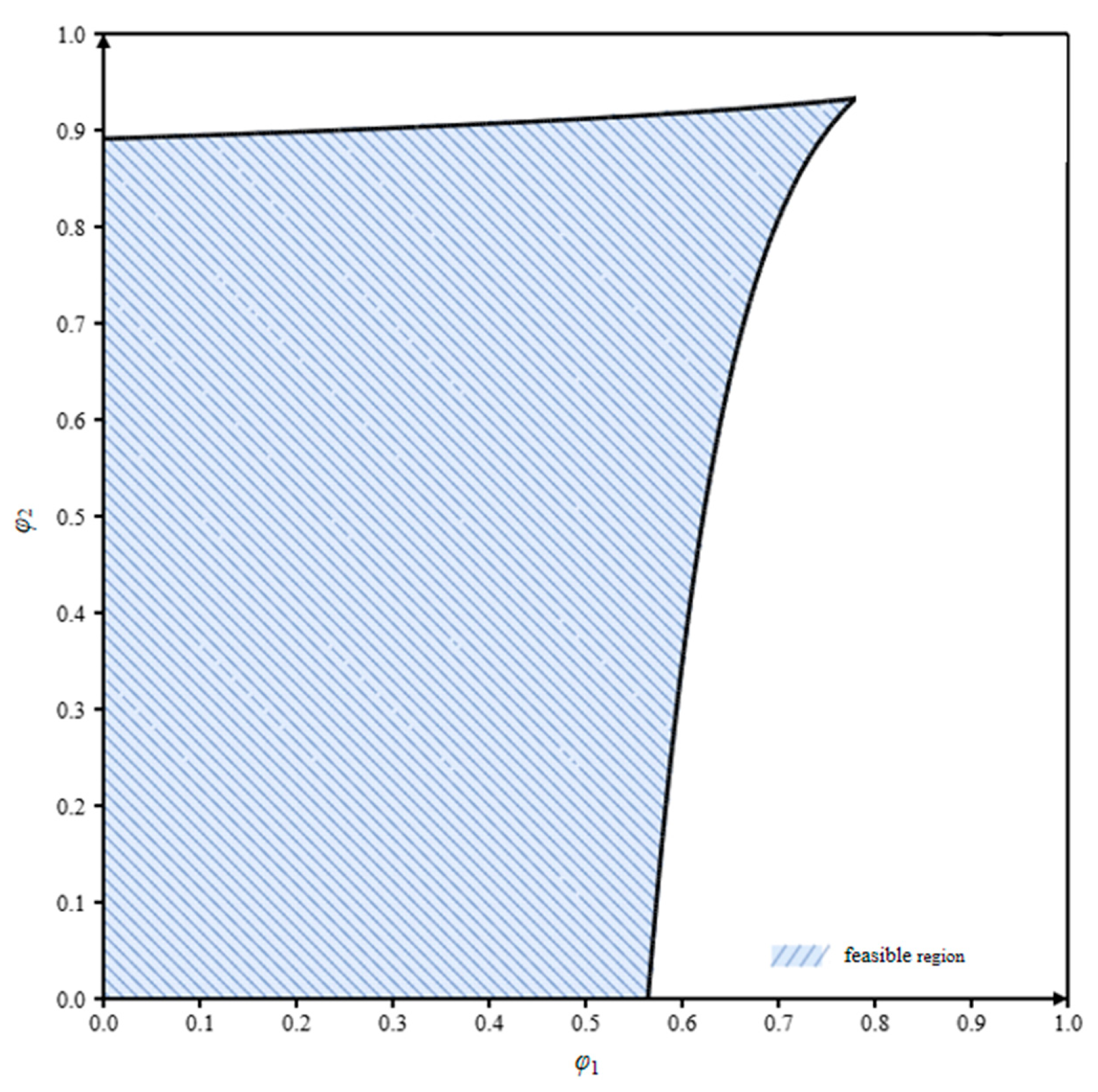
Although an increase in the cost-sharing ratio can make the endurance and marketing strategies more efficient and increase eVTOL brand goodwill and demand, an excessive cost-sharing ratio will damage the profits of the manufacturer and retailer. Therefore, the manufacturer and retailer need to negotiate under the two-way cost-sharing contract, so that a Pareto improvement can be achieved, and $\left\{\begin{array}{l}{J}_m^S\left({\phi }_1,{\phi }_2\right)\ge J_m^N\hfill \\ J_r^S\left({\phi }_1,{\phi }_2\right)\ge J_r^N\hfill \end{array}\right.$ must be satisfied. We substitute other parameter assignments into this inequality and obtain the feasible region for the cost-sharing proportions φ₁, φ₂. Figure 1 shows the feasible region of φ₁, φ₂ through shading.

4. Numerical Illustration

In this section, we perform numerical simulations using specific values to verify the conclusions derived from the mathematical model and to illustrate the dynamic processes that are difficult to capture in detail through mathematical derivations. Following the relevant literature and selected practical references [27,30,34], we assign economically meaningful values to the parameters: μ = 0.4, λ = 0.5, δ = 0.2, γ = 0.5, α = 150, β = 1, k_m = 1, k_r = 1, c = 130, ρ = 0.3, φ₁ = 0.2, φ₂ = 0.2, s = 10, and G₀ = 0.5. We conduct a systematic sensitivity analysis of the parameter values, and the results are shown in Appendix B. The values of the relevant parameters do not affect the conclusions of this study.

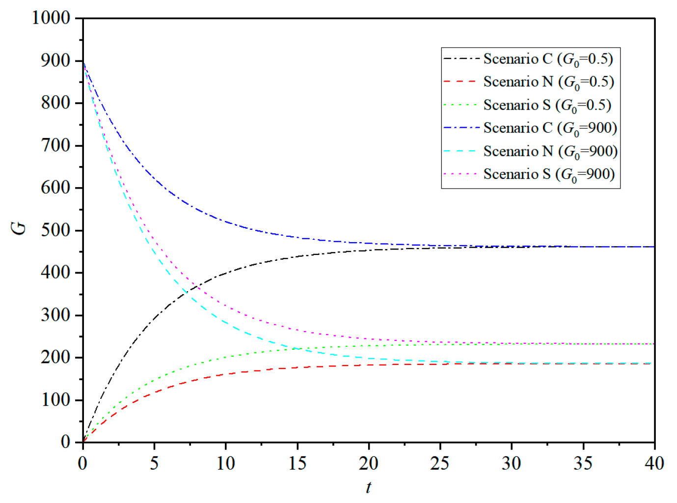
In order to describe the dynamic evolution trajectory of eVTOL brand goodwill, two cases of initial brand goodwill, G₀ = 0.5 and G₀ = 900, are selected to analyze their convergence process in Scenarios C, N, and S.

Figure 2 shows the trajectory of eVTOL brand goodwill. In terms of trend, the time evolution trajectory of brand goodwill is related to the initial value: when the initial brand goodwill is low, that in Scenarios C, N, and S increases over time and eventually converges to a steady-state level; when the initial brand goodwill is high, that in Scenarios C, N, and S gradually decreases and converges to a steady state. Therefore, the steady-state level of brand goodwill is independent of the initial brand goodwill and depends solely on the business model. In terms of the steady-state level, the relationship between brand goodwill among the three scenarios is $G^C>G^S>G^N$; the steady-state value of brand goodwill in Scenario C is the highest, followed by that in Scenarios S and N. Corollary (5) is proven, indicating that brand goodwill is affected by the double-marginalization effect under the decentralized decision-making model and is lower than that under the centralized decision-making model; however, the two-way cost-sharing contract can effectively improve brand goodwill under decentralized decision-making.

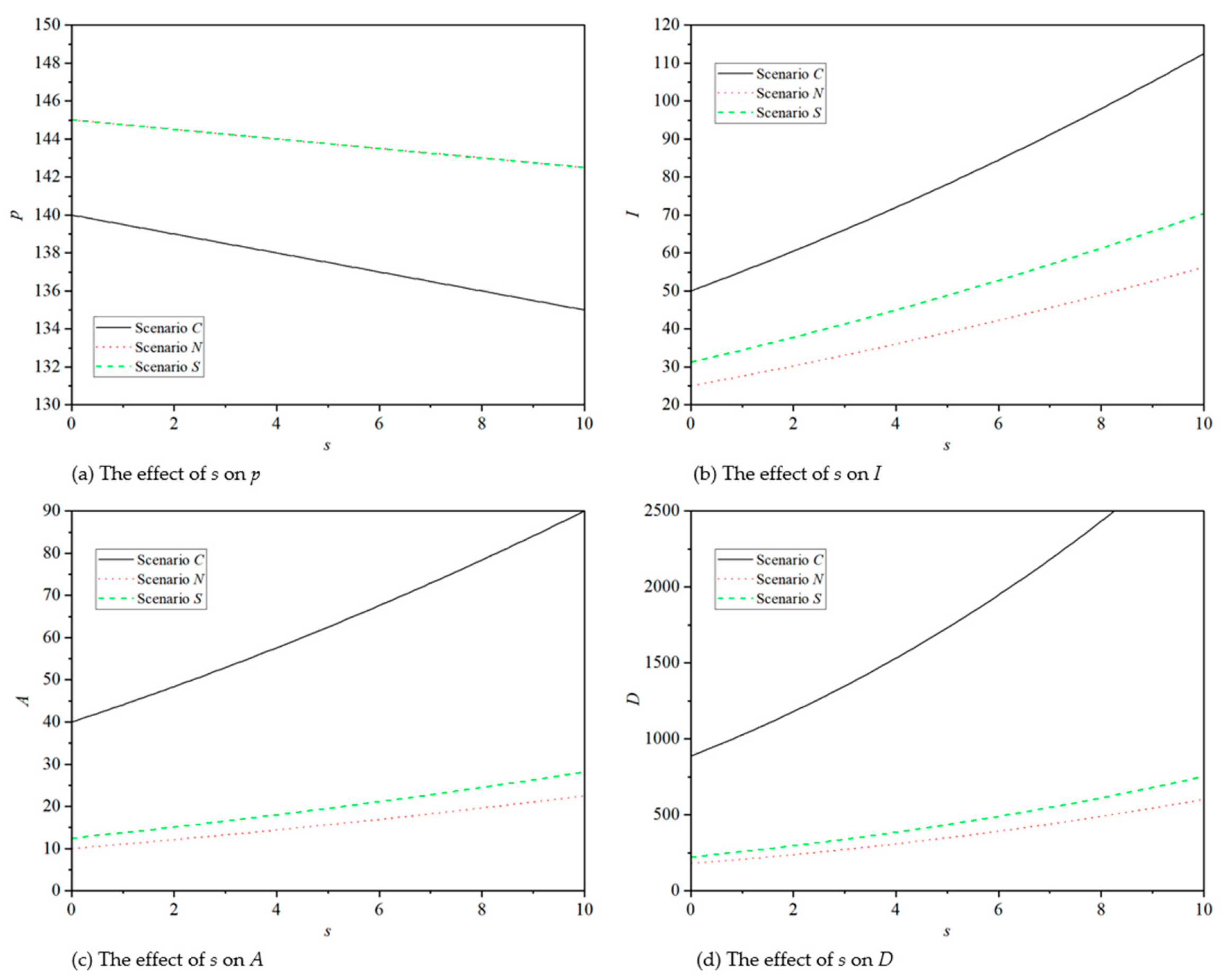
By changing the eVTOL subsidy rate s and keeping other parameters the same, we can obtain the change rules of the eVTOL retail price, endurance effort, marketing effort, and demand with respect to s, as shown in Figure 3. Regarding the trend, the eVTOL retail price decreases, while the endurance effort, marketing effort, and demand increase, with an increase in s, which is consistent with the earlier comparative static analysis results. Concerning levels, the relationships between the eVTOL retail price, endurance effort, marketing effort, and demand in the three scenarios are $p^C<p^N=p^S$ (Figure 3a), $I^C>I^S>I^N$ (Figure 3b), $A^C>A^S>A^N$ (Figure 3c), and $D^C>D^S>D^N$ (Figure 3d); these verify Corollaries (1), (2), (3), and (6). Compared to decentralized decision-making, a manufacturer and retailer operating under centralized decision-making set a lower sales price but invest more in endurance effort and marketing effort. Consequently, these higher efforts, combined with lower sales prices, in the centralized decision-making supply chain lead to higher sales volumes.

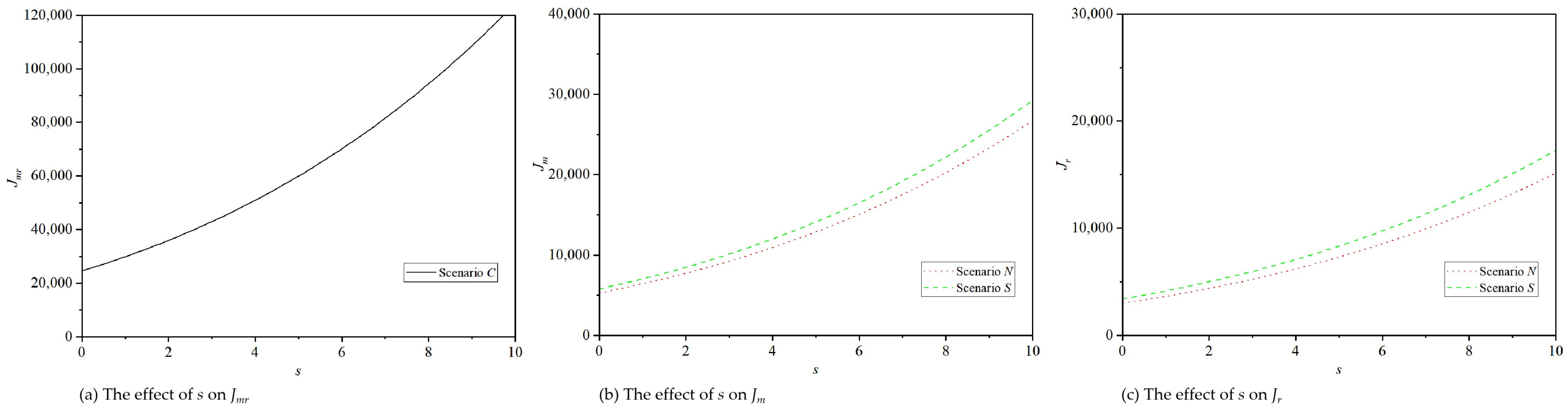
Figure 4 shows the variations in J_mr, J_m, and J_r with respect to s. It can be seen that, under centralized decision-making, the eVTOL supply chain profit J_mr is positively correlated with the subsidy rate s (Figure 4a); under decentralized decision-making, the subsidy rate has a positive impact on the profits of the manufacturer and retailer, which increase with an increase in the subsidy rate (Figure 4b,c). In addition, when the cost-sharing proportions φ₁ and φ₂ are within the feasible region in the test range, the profits of the manufacturer and the retailer under decentralized decision-making are higher with the cost-sharing contract than without cost-sharing (Figure 4b,c). However, the sum of the supply chain members’ profits after coordination cannot reach the supply chain profit under centralized decision-making; there is still a gap. Therefore, although the two-way cost-sharing contract enables the supply chain members to achieve a Pareto improvement, it cannot achieve Pareto optimality.

5. Discussion

5.1. Extension of the Basic Model

The previous section constructs a supply chain model including a manufacturer and a retailer. This section further extends the benchmark model by considering a supply chain composed of two manufacturers (i = 1, 2) producing subjunctive eVTOL products and a retailer selling two products [35]. The two manufacturers, as Stackelberg leaders of the supply chain system, first choose the optimal endurance effort I_i and the wholesale price w_i, and the Bertrand game takes place simultaneously between them. The retailer is the follower and subsequently chooses the optimal marketing effort A_i and the retail price p_i for the two products. The objective functions of manufacturer i and the retailer are expressed as

$$\max J_{im}^N\left(t\right)={\displaystyle {\int }_0^{\infty }{e}^{-\rho t}\left[\left(w_i-c_i+s\right)D_i-C_{im}\right]dt}$$

(12)

$$\max J_r^N\left(t\right)={\displaystyle {\int }_0^{\infty }{e}^{-\rho t}{\displaystyle \sum _{i=1}^2\left[\left(p_i-w_i\right)D_i-C_{ir}\right]}dt}$$

(13)

where $C_{1m}={\displaystyle \frac{k_{1m}{I}_1^2}{2}}$, $C_{2m}={\displaystyle \frac{k_{2m}{I}_2^2}{2}}$, $C_{1r}={\displaystyle \frac{k_r{A}_1^2}{2}}$, $C_{2r}={\displaystyle \frac{k_r{A}_2^2}{2}}$, $D_1=\gamma G_1({\alpha }_1-{\beta }_1{p}_1+{\chi }_1{p}_2)$, and $D_2=\gamma G_2({\alpha }_2-{\beta }_2{p}_2+{\chi }_2{p}_1)$.

We solve the above equations and obtain the feedback Stackelberg equilibrium results.

The results are as follows for manufacturer 1:

(1)

The optimal endurance effort is $I_1^N={\displaystyle \frac{\lambda V_{1m}^N}{k_{1m}}}$.

(2)

The wholesale price is $w_1^N={\displaystyle \frac{2\Gamma {\Psi }_1+{\chi }_1{\beta }_2{\Psi }_2}{4{\Gamma }^2-{\beta }_1{\beta }_2{\chi }_1{\chi }_2}}$.

(3)

The present value profit function is $J_{1m}^N=V_{1m}^N{G}_1^N+{\displaystyle \frac{1}{\rho }}\left\{{\displaystyle \frac{{\lambda }^2{\left(V_{1m}^N\right)}^2}{2k_{1m}}}+{\displaystyle \frac{{\mu }^2{V}_{1m}^N{V}_{1r}^N}{k_r}}\right\}$.

The results are as follows for manufacturer 2:

(1)

The optimal endurance effort is $I_2^N={\displaystyle \frac{\lambda V_{2m}^N}{k_{2m}}}$.

(2)

The wholesale price is $w_2^N={\displaystyle \frac{2\Gamma {\Psi }_2+{\chi }_2{\beta }_1{\Psi }_1}{4{\Gamma }^2-{\beta }_1{\beta }_2{\chi }_1{\chi }_2}}$.

(3)

The present value profit function is $J_{2m}^N=V_{2m}^N{G}_2^N+{\displaystyle \frac{1}{\rho }}\left\{{\displaystyle \frac{{\lambda }^2{\left(V_{2m}^N\right)}^2}{2k_{2m}}}+{\displaystyle \frac{{\mu }^2{V}_{2m}^N{V}_{2r}^N}{k_r}}\right\}$.

The results are as follows for the retailer:

(1)

The optimal marketing effort of eVTOL product 1 is $A_1^N={\displaystyle \frac{\mu V_{1r}^N}{k_r}}$, and that of eVTOL product 2 is $A_2^N={\displaystyle \frac{\mu V_{2r}^N}{k_r}}$.

(2)

The retail price of eVTOL product 1 is $p_1^N={\displaystyle \frac{2{\beta }_2\left({\alpha }_1+{\beta }_1{w}_1\right)+{\chi }_1\left({\alpha }_2+{\beta }_2{w}_2\right)}{4{\beta }_1{\beta }_2-{\chi }_1{\chi }_2}}$, and that of eVTOL product 2 is $p_2^N={\displaystyle \frac{2{\beta }_1\left({\alpha }_2+{\beta }_2{w}_2\right)+{\chi }_2\left({\alpha }_1+{\beta }_1{w}_1\right)}{4{\beta }_1{\beta }_2-{\chi }_1{\chi }_2}}$.

(3)

The retailer’s present value profit function is

$$J_r^N=V_{1r}^N{G}_1^N+V_{2r}^N{G}_2^N+{\displaystyle \frac{1}{\rho }}\left\{{\displaystyle \frac{{\mu }^2{\left(V_{1r}^N\right)}^2}{2k_r}}+{\displaystyle \frac{{\lambda }^2{V}_{1m}^N{V}_{1r}^N}{k_{1m}}}+{\displaystyle \frac{{\mu }^2{\left(V_{2r}^N\right)}^2}{2k_r}}+{\displaystyle \frac{{\lambda }^2{V}_{2m}^N{V}_{2r}^N}{k_{2m}}}\right\}$$

Based on the above equations, the brand goodwill of eVTOL product 1 is $G_1^N=G_{10}^N{e}^{-\delta t}+G_{1\infty }^N\left(1-e^{-\delta t}\right)$ and the demand is $D_1^N=\gamma G_1^N\left[{\alpha }_1-{\beta }_1{p}_1+{\chi }_1{p}_2\right]$, while the brand goodwill of eVTOL product 2 is $G_2^N=G_{20}^N{e}^{-\delta t}+G_{2\infty }^N\left(1-e^{-\delta t}\right)$ and the demand is $D_2^N=\gamma G_2^N\left[{\alpha }_2-{\beta }_2{p}_2+{\chi }_2{p}_1\right]$, where $G_{1\infty }^N={\displaystyle \frac{\mu A_1^N+\lambda I_1^N}{\delta }}$, $G_{2\infty }^N={\displaystyle \frac{\mu A_2^N+\lambda I_2^N}{\delta }}$, $\Gamma =2{\beta }_1{\beta }_2-{\chi }_1{\chi }_2$, ${\Psi }_1=2{\alpha }_1{\beta }_2+{\chi }_1{\alpha }_2+\Gamma \left(c_1-s\right)$, ${\Psi }_2=2{\alpha }_2{\beta }_1+{\chi }_2{\alpha }_1+\Gamma \left(c_2-s\right)$, $V_{1m}^N={\displaystyle \frac{\gamma \left({\alpha }_1-{\beta }_1{p}_1+{\chi }_1{p}_2\right)\left(w_1-c_1+s\right)}{\left(\rho +\delta \right)}}$, $V_{2m}^N={\displaystyle \frac{\gamma \left({\alpha }_2-{\beta }_2{p}_2+{\chi }_2{p}_1\right)\left(w_2-c_2+s\right)}{\left(\rho +\delta \right)}}$, $V_{1r}^N={\displaystyle \frac{\gamma \left({\alpha }_1-{\beta }_1{p}_1+{\chi }_1{p}_2\right)\left(p_1-w_1\right)}{\left(\rho +\delta \right)}}$, $V_{2r}^N={\displaystyle \frac{\gamma \left({\alpha }_2-{\beta }_2{p}_2+{\chi }_2{p}_1\right)\left(p_2-w_2\right)}{\left(\rho +\delta \right)}}$.

When ${\chi }_1=0$, ${\chi }_2=0$, the above model will degenerate into the benchmark model. In the supply chain composed of two manufacturers and one retailer, it is easy to prove that ${\displaystyle \frac{\partial w_1^N}{\partial s}}<0$, ${\displaystyle \frac{\partial w_2^N}{\partial s}}<0$, ${\displaystyle \frac{\partial p_1^N}{\partial s}}<0$, ${\displaystyle \frac{\partial p_2^N}{\partial s}}<0$, ${\displaystyle \frac{\partial I_1^N}{\partial s}}>0$, ${\displaystyle \frac{\partial I_2^N}{\partial s}}>0$, ${\displaystyle \frac{\partial A_1^N}{\partial s}}>0$, ${\displaystyle \frac{\partial A_2^N}{\partial s}}>0$, ${\displaystyle \frac{\partial G_1^N}{\partial s}}>0$, ${\displaystyle \frac{\partial G_2^N}{\partial s}}>0$, ${\displaystyle \frac{\partial D_1^N}{\partial s}}>0$, ${\displaystyle \frac{\partial D_2^N}{\partial s}}>0$. In other words, the eVTOL subsidy rate has a negative impact on the wholesale and retail prices and a positive impact on the endurance and marketing efforts, brand goodwill, and demand. This is consistent with the conclusions of the benchmark model, indicating the robustness of the research conclusions. The subsidy rate is not affected by the competitive structure of the upstream market. The government subsidy increases the unit profit margin of the manufacturer producing eVTOL, who can then lower the wholesale price; the subsidy also encourages the manufacturer and retailer to increase their endurance and marketing investments, respectively. Higher R&D and marketing investments accelerate the accumulation of brand goodwill, and the dual role of goodwill improvement and product price reduction drives the expansion of the market demand.

5.2. Optimal Subsidy Rate Considering the Maximization of Social Welfare

Government subsidies to make eVTOL affordable to consumers require a large amount of fiscal expenditure and may lead to social welfare losses, while eVTOL simultaneously brings high emissions compared to high-frequency battery replacements in ground vehicles. Therefore, the government faces a practical problem: how should the subsidy level be set to encourage profit-maximizing enterprises to increase their investments in endurance R&D while improving overall social welfare? To this end, we further study the optimal subsidy rate of the supply chain when the government aims to maximize social welfare [36]. The social welfare function is defined as the sum of profit for the manufacturer and retailer, the net consumer surplus of government subsidy expenditure, and environmental damage, i.e., $SW\left(t\right)={\pi }_m\left(t\right)+{\pi }_r\left(t\right)+CS\left(t\right)-ED\left(t\right)-FS\left(t\right)$, where ${\pi }_m\left(t\right)$ is the manufacturer’s profit (Equation (14)); ${\pi }_r\left(t\right)$ is the retailer’s profit (Equation (15)); $CS\left(t\right)$ is the consumer surplus (Equation (16)); $ED\left(t\right)$ is the environmental damage cost (Equation (17)); σ is the unit environmental damage cost; and $FS\left(t\right)$ is the fiscal subsidy given by the government to the manufacturer (Equation (18)).

$${\pi }_m\left(t\right)=\left[w\left(t\right)-c\left(t\right)+s\left(t\right)\right]D\left(t\right)-C_m\left(t\right)$$

(14)

$${\pi }_m\left(t\right)=\left[w\left(t\right)-c\left(t\right)+s\left(t\right)\right]D\left(t\right)-C_m\left(t\right)$$

(15)

$$CS\left(t\right)={\displaystyle {\int }_0^{\infty }D\left(p\left(t\right),G\left(t\right)\right)dp}\left(t\right)={\displaystyle \frac{\gamma G\left(t\right){\left(\alpha -\beta p\left(t\right)\right)}^2}{2\beta }}$$

(16)

$$ED\left(t\right)=\sigma D\left(t\right)$$

(17)

$$FS\left(t\right)=sD\left(t\right)$$

(18)

Under the centralized decision-making model, the decision sequence is as follows: the government sets the optimal subsidy rate, and then the supply chain determines the optimal values for the endurance effort, marketing effort, and sales price. Under the decentralized decision-making model, the sequence is as follows: the government sets the optimal subsidy rate, the manufacturer selects the optimal values for the endurance effort and wholesale price, and then the retailer selects the optimal marketing effort and retail price. In Scenarios C, N, and S, the objective functions based on maximizing social welfare are as follows:

$$\max J_{SW}^C\left(t\right)={\displaystyle {\int }_0^{\infty }{e}^{-\rho t}\left[\left(w-c+s\right)D-C_m+\left(p-w\right)D-C_r+CS-ED-FS\right]dt}$$

(19)

$$\max J_{SW}^N\left(t\right)={\displaystyle {\int }_0^{\infty }{e}^{-\rho t}\left[\left(w-c+s\right)D-C_m+\left(p-w\right)D-C_r+CS-ED-FS\right]dt}$$

(20)

$$\max J_{SW}^S\left(t\right)={\displaystyle {\int }_0^{\infty }{e}^{-\rho t}\left[\left(w-c+s\right)D-C_m+\left(p-w\right)D-C_r+CS-ED-FS\right]dt}$$

(21)

Combining Equations (7)–(11), we solve the above equations to obtain the optimal government subsidy rate for eVTOL under the different scenarios:

(1)

In Scenario C, the optimal subsidy rate of the government is $s^C={\displaystyle \frac{\alpha }{\beta }}-c-2\sigma$.

(2)

In Scenario N, the optimal subsidy rate of the government is $s^N={\displaystyle \frac{3\alpha }{\beta }}-3c-4\sigma$.

(3)

In Scenario S, the optimal subsidy rate of the government is $s^S={\displaystyle \frac{3\alpha }{\beta }}-3c-4\sigma$.

It can be seen that the optimal subsidy is jointly affected by α, β, c and σ: the larger α is, the higher the optimal subsidy, and the larger β, c, and σ are, the lower the optimal subsidy. It is not surprising that the optimal subsidy level depends on the market size of eVTOL: a small subsidy, rather than a large subsidy, can leverage demand when consumers are more price-sensitive. The lifecycle emissions of eVTOL are significantly higher than those of ICEVs, BEVs, and PHEVs, due to the high emissions resulting from their long operational range and frequent battery replacement; blindly increasing the subsidy to expand the market will exacerbate the environmental burden. The impact of the production cost on the optimal subsidy level may seem somewhat counterintuitive, as the research and manufacturing costs of eVTOL are relatively high, and the government provides a subsidy to reduce the corporate cost and encourage capacity expansion. However, a higher production cost means that more resources are consumed in the production of eVTOL, and such a subsidy should not be encouraged at high levels. Additionally, the optimal subsidy level for maximizing social welfare under the centralized decision-making model is significantly lower than that under the decentralized one. The centralized decision-making supply chain achieves integration, and there is no double-marginalization effect: the virtual central decision-maker internally coordinates the wholesale price, retail price, endurance effort, and marketing effort; thus, enterprises spontaneously eliminate the distortion of channel markup, and the government can achieve optimal social welfare with only a modest subsidy.

5.3. Carbon Trading Policy as Alternative to Subsidy Policy

Once the eVTOL industry reaches a certain stage of development and the market gains the capacity to expand, government subsidy will be phased out according to the plan until it is completely eliminated, so as to facilitate the industry’s transition from policy- to market-driven. Upon reviewing the development of the new energy vehicle industry, the Chinese government proposed a corporate average fuel consumption (CAFC) and new energy vehicle (NEV) credit policy to replace fiscal subsidies. CAFC-NEV credits promote the development of the new energy vehicle industry; however, with the improvement in the penetration rate of new energy vehicles, the role that the CAFC-NEV credit policy can play is significantly weakened. In this context, the Ministry of Industry and Information Technology proposes transforming the CAFC-NEV credit policy into a carbon emission management policy. Academic research on carbon emission management policies is mainly divided into research on carbon taxes and the carbon market, where the latter includes the compliance carbon market (ETS) and voluntary carbon market (CER). China has implemented national carbon emissions trading without a carbon tax. The Nationally Determined Contribution Report of China in 2035 states that the carbon market has become the main method for carbon pricing in China. Related research shows that carbon taxes may cause welfare losses [37], and the academic community is cautious about introducing it. Therefore, we use a carbon trading policy as an alternative to eVTOL subsidies. Based on the allocation of national carbon market quotas, a bottom-up quota allocation method is adopted, in which the quotas for each controlled emission entity are determined according to the quota allocation rules and then summed to obtain the upper limit of the total quota for the system. According to the earlier analysis, the introduction of cost-sharing contracts does not change the basic conclusions regarding the subsidy policy under decentralized decision-making; thus, this section only analyzes the impacts of the carbon trading policy under centralized decision-making and decentralized decision-making without cost-sharing.

Under the centralized decision-making model, the objective function of the entire supply chain is

$$\max J_{mr}^C\left(t\right)={\displaystyle {\int }_0^{\infty }{e}^{-\rho t}\left[\left(w-c\right)D-C_m+\left(p-w\right)D-C_r+p_c\left(Q-\Phi \right)D\right]dt}$$

(22)

where p_c represents the carbon trading price, Q represents the carbon quota, and Φ represents the carbon emissions during the lifecycle of eVTOL.

We solve the above equation and obtain the feedback Stackelberg equilibrium results.

(1)

The optimal endurance effort is $I^C={\displaystyle \frac{\lambda \gamma {\left\{\alpha -\beta \left[c-\left(p_{c}Q-p_c\Phi \right)\right]\right\}}^2}{k_{m}4\beta \left(\rho +\delta \right)}}$, the optimal marketing effort is $A^C={\displaystyle \frac{\mu \gamma {\left\{\alpha -\beta \left[c-\left(p_{c}Q-p_c\Phi \right)\right]\right\}}^2}{k_{r}4\beta \left(\rho +\delta \right)}}$, and the retail price is $p^C={\displaystyle \frac{\alpha +\beta \left[c-\left(p_{c}Q-p_c\Phi \right)\right]}{2\beta }}$.

(2)

The trajectory of eVTOL brand goodwill for the manufacturer is $G^C=G_0^C{e}^{-\delta t}+G_{\infty }^C\left(1-e^{-\delta t}\right)$, where $G_{\infty }^C={\displaystyle \frac{\mu A^C+\lambda I^C}{\delta }}$.

(3)

The optimal demand for eVTOL is $D^C={\displaystyle \frac{\gamma G^C\left\{\alpha -\beta \left[c-\left(p_{c}Q-p_c\Phi \right)\right]\right\}}{2}}$.

(4)

The present value profit function of the supply chain is

$$J_{mr}^C={\displaystyle \frac{\gamma {\left\{\alpha -\beta \left[c-\left(p_{c}Q-p_c\Phi \right)\right]\right\}}^2}{4\beta \left(\rho +\delta \right)}}{G}^C+{\displaystyle \frac{1}{\rho }}\left\{{\displaystyle \frac{\left({\lambda }^2{k}_r+{\mu }^2{k}_m\right){\gamma }^2{\left\{\alpha -\beta \left[c-\left(p_{c}Q-p_c\Phi \right)\right]\right\}}^4}{2k_m{k}_{r}16{\beta }^2{\left(\rho +\delta \right)}^2}}\right\}$$

Under decentralized decision-making without cost-sharing, assuming that the manufacturer and retailer share or bear a certain proportion of the carbon quota surplus revenue and compliance cost, their objective functions are, respectively, expressed as

$$\max J_m^N\left(t\right)={\displaystyle {\int }_0^{\infty }{e}^{-\rho t}\left[\left(w-c\right)D-C_m+\theta p_c\left(Q-\Phi \right)D\right]dt}$$

(23)

$$\max J_m^N\left(t\right)={\displaystyle {\int }_0^{\infty }{e}^{-\rho t}\left[\left(w-c\right)D-C_m+\theta p_c\left(Q-\Phi \right)D\right]dt}$$

(24)

where θ represents the proportion of the carbon trading cost or benefit shared by the manufacturer.

We solve the above equations and obtain the feedback Stackelberg equilibrium results.

(1)

The optimal endurance effort is $I^N={\displaystyle \frac{\lambda \gamma \left[w-c+\theta \left(p_{c}Q-p_c\Phi \right)\right]\left[\alpha -\beta w+\beta \left(1-\theta \right)\left(p_{c}Q-p_c\Phi \right)\right]}{k_{m}2\left(\rho +\delta \right)}}$.

(2)

The wholesale price is $w^N={\displaystyle \frac{\alpha +\beta \left[c-\left(2\theta -1\right)\left(p_{c}Q-p_c\Phi \right)\right]}{2\beta }}$.

(3)

The optimal marketing effort is $A^N={\displaystyle \frac{\mu \gamma {\left[\alpha -\beta w+\beta \left(1-\theta \right)\left(p_{c}Q-p_c\Phi \right)\right]}^2}{k_{r}4\beta \left(\rho +\delta \right)}}$.

(4)

The retail price is $p^N={\displaystyle \frac{3\alpha +\beta \left[c-\left(p_{c}Q-p_c\Phi \right)\right]}{4\beta }}$.

(5)

The trajectory of eVTOL brand goodwill is $G^N=G_0^N{e}^{-\delta t}+G_{\infty }^N\left(1-e^{-\delta t}\right)$, where $G_{\infty }^N={\displaystyle \frac{\mu A^N+\lambda I^N}{\delta }}$.

(6)

The optimal demand for eVTOL is $D^N={\displaystyle \frac{\gamma G^N\left\{\alpha -\beta \left[c-\left(p_{c}Q-p_c\Phi \right)\right]\right\}}{4}}$.

(7)

The present value profit functions for the manufacturer and retailer, respectively, are

$$J_m^N={\displaystyle \frac{\gamma \left[\begin{array}{c}w-c+\\ \theta \left(p_{c}Q-p_c\Phi \right)\end{array}\right]\left[\begin{array}{c}\alpha -\beta w+\\ \beta (1-\theta )\left(p_{c}Q-p_c\Phi \right)\end{array}\right]}{2(\rho +\delta )}}{G}^N+{\displaystyle \frac{1}{\rho }}\left\{\begin{array}{c}{\left[\begin{array}{c}\gamma \left[\begin{array}{c}w-c+\\ \theta \left(p_{c}Q-p_c\Phi \right)\end{array}\right]\left[\begin{array}{c}\alpha -\beta w+\\ \beta (1-\theta )\left(p_{c}Q-p_c\Phi \right)\end{array}\right]\\ 2(\rho +\delta )\end{array}\right]}^2{\displaystyle \frac{{\lambda }^2}{2k_m}}\\ +{\displaystyle \frac{{\mu }^2{\gamma }^2{\left[\begin{array}{c}\alpha -\beta w+\\ \beta (1-\theta )\left(p_{c}Q-p_c\Phi \right)\end{array}\right]}^3\left[\begin{array}{c}w-c+\\ \theta \left(p_{c}Q-p_c\Phi \right)\end{array}\right]}{8\beta k_r{(\rho +\delta )}^2}}\end{array}\right\}$$

$$J_r^N={\displaystyle \frac{\gamma {\left[\begin{array}{c}\alpha -\beta w+\\ \beta (1-\theta )\left(p_{c}Q-p_c\Phi \right)\end{array}\right]}^2}{4\beta (\rho +\delta )}}{G}^N+{\displaystyle \frac{1}{\rho }}\left\{\begin{array}{c}{\displaystyle \frac{{\mu }^2}{2k_r}}{\{{\displaystyle \frac{\gamma {\left[\begin{array}{c}\alpha -\beta w+\\ \beta (1-\theta )\left(p_{c}Q-p_c\Phi \right)\end{array}\right]}^2}{4\beta (\rho +\delta )}}]}^2+\\ {\displaystyle \frac{{\lambda }^2{\gamma }^2\left[\begin{array}{c}w-c+\\ \theta \left(p_{c}Q-p_c\Phi \right)\end{array}\right]{\left[\begin{array}{c}\alpha -\beta w+\\ \beta (1-\theta )\left(p_{c}Q-p_c\Phi \right)\end{array}\right]}^3}{8\beta k_m{(\rho +\delta )}^2}}\end{array}\right\}$$

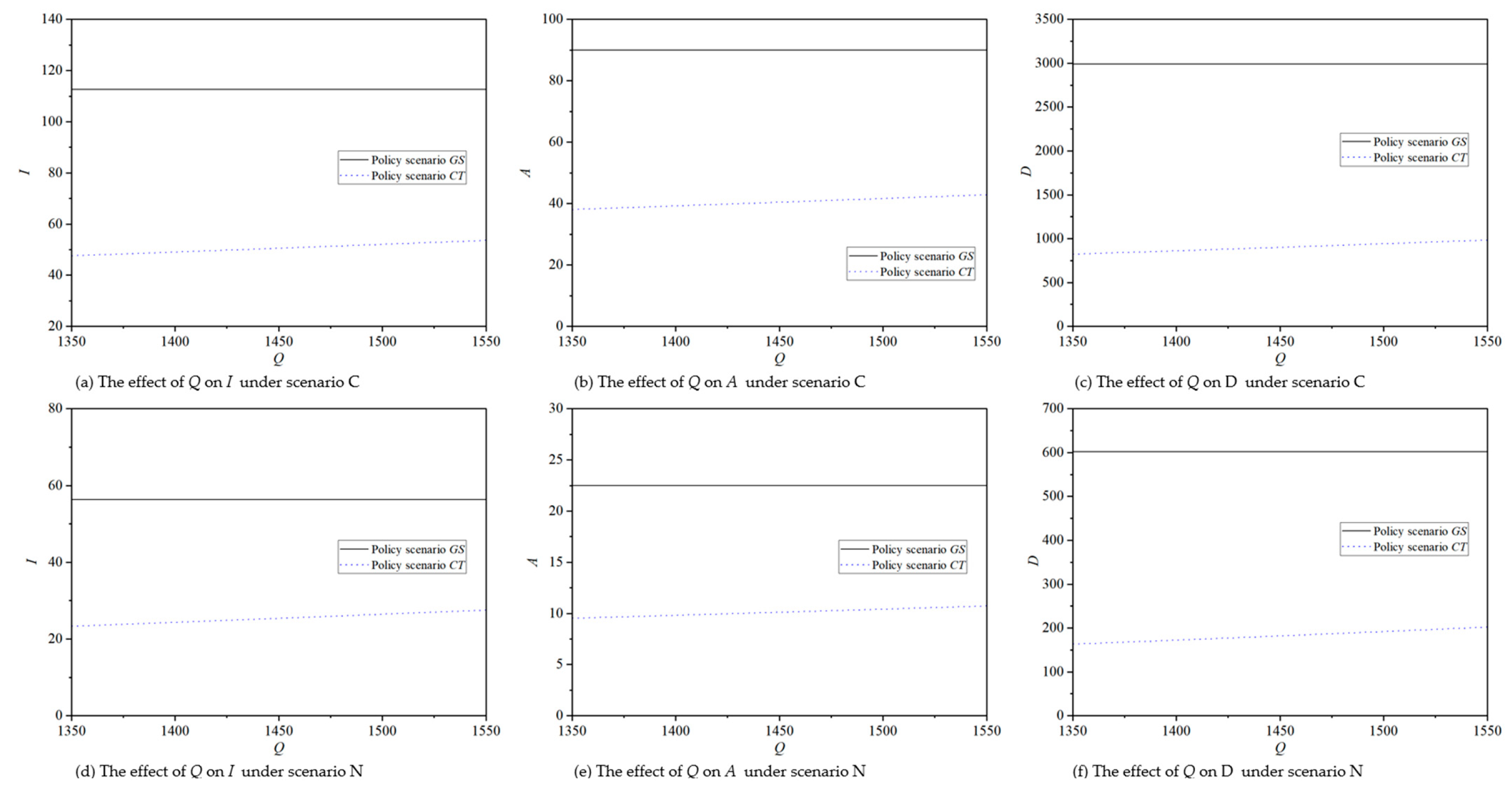
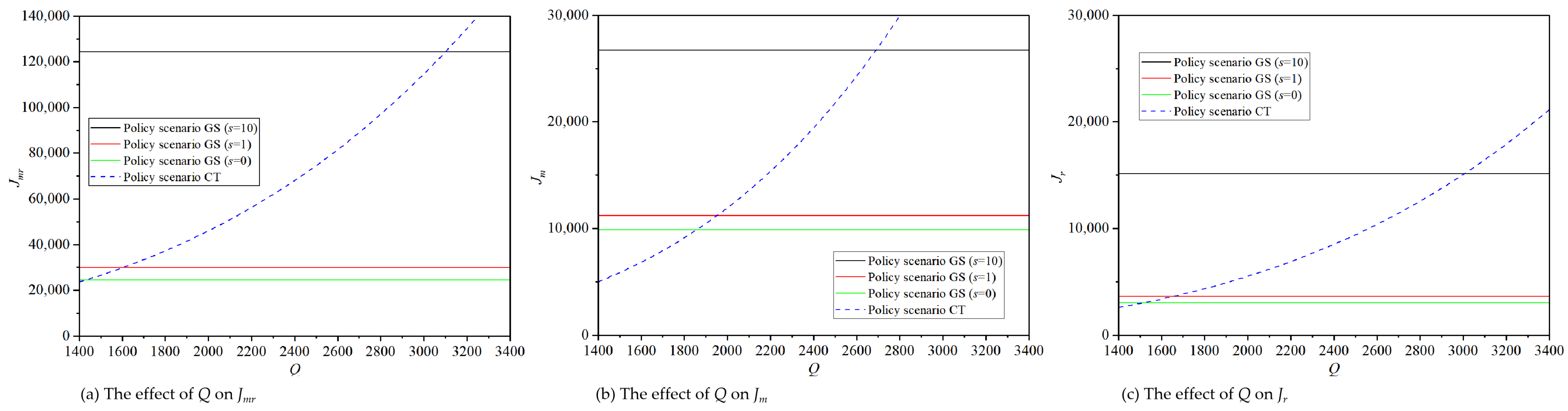
Based on the above-mentioned assignment, the parameter settings related to the carbon trading policy are as follows: p_c = 0.006, Q = 1400, and Φ = 1433. The carbon price follows the average trading price of CEA in the national carbon market in 2025, and the unit is ten thousand yuan. The lifecycle carbon emissions of eVTOL are measured in tons according to the research by Liu et al. [38], and the carbon quota is slightly lower than the actual carbon emissions; a sensitivity analysis is subsequently carried out. Figure 5 and Figure 6 illustrate the endurance effort, marketing effort, demand, and profit under the government subsidy (GS) and carbon trading (CT) policies in Scenarios C and N.

We change the carbon quota Q and keep other parameters the same to obtain the change rules of the endurance effort, marketing effort, demand, and profit with respect to Q. Regarding the trend, the endurance effort, marketing effort, demand, and profit increase with an increase in Q for Scenarios C and N. Therefore, under the carbon trading policy framework, which adopts lifecycle carbon emission accounting and shares the carbon performance cost proportionally between the manufacturer and retailer, raising the carbon quota will drive an increase in the eVTOL manufacturer’s endurance effort and the retailer’s marketing effort in step with the market demand. A higher carbon quota can reduce the overall carbon quota expenditure of the supply chain and alleviate the carbon performance burden of the whole chain, covering production and operation. As the carbon cost is shared by upstream and downstream subjects, the carbon expenditure borne by the manufacturer decreases, the marginal profit improves, and there are sufficient funds to carry out endurance R&D. Meanwhile, endurance effort can reduce energy consumption during flight, lower carbon emissions over the whole lifecycle, further reduce the carbon cost, and encourage the manufacturer to improve this effort further. For the retailer, the downward trend of the upstream carbon cost drives down the wholesale price, as well as reducing the shared carbon cost, expanding the retail profit space per unit product, and increasing the revenue achieved through marketing investment, thus promoting an increase in marketing effort. In addition, a lower carbon quota leads to a decline in retail price, and superimposed endurance R&D and marketing activities jointly drive the accumulation of brand goodwill, driving the expansion of the eVTOL market demand.

Within the parameters tested in this study, the endurance effort, marketing effort, and demand are lower under the carbon trading policy than under the subsidy policy (Figure 5). However, if the carbon quota is sufficiently high or the lifecycle carbon emissions decrease substantially, these factors will reach or even exceed the levels of those under the subsidy policy, as shown in

Table 5. The sensitivity analysis of s and Q in Scenarios C and N.

	s = 2	s = 4	s = 6	s = 8	s = 10	Q = 1400	Q = 1600	Q = 1800	Q = 2000	Q = 2200
pC	139.0	138.0	137.0	136.0	135.0	140.1	139.5	138.9	138.3	137.7
IC	60.5	72.0	84.5	98.0	112.5	49.0	55.1	61.6	68.5	75.7
AC	48.4	57.6	67.6	78.4	90.0	39.2	44.1	49.3	54.8	60.5
GC	214.5	255.3	299.6	347.5	398.9	173.8	195.5	218.5	242.8	268.3
DC	1180.0	1531.9	1947.6	2432.4	2991.7	860.6	1026.6	1212.8	1420.2	1650.1
$J_{mr}^C$	35,965.0	50,935.2	70,154.3	94,359.0	124,345.0	23,607.4	29,870.4	37,304.0	46,045.7	56,240.7
pN	144.5	144.0	143.5	143.0	142.5	145.0	144.7	144.4	144.1	143.8
wN	139.0	138.0	137.0	136.0	135.0	140.0	139.9	139.8	139.7	139.5
IN	30.3	36.0	42.3	49.0	56.3	24.5	27.6	30.8	34.2	37.8
AN	12.1	14.4	16.9	19.6	22.5	9.8	11.0	12.3	13.7	15.1
GN	86.4	102.8	120.6	139.9	160.6	70.0	78.7	88.0	97.7	108.0
DN	237.6	308.4	392.0	489.6	602.1	173.3	206.7	244.2	285.9	332.2
$J_m^N$	7727.3	10,943.3	15,071.9	20,271.4	26,712.7	5072.6	6418.1	8015.0	9892.9	12,083.0
$J_r^N$	4382.2	6206.0	8547.5	11,496.2	15,149.3	2876.6	3639.7	4545.3	5610.3	6852.4

. Studies have shown that the lifecycle carbon emissions of eVTOL are as high as 1433 tons, mainly due to high emissions from high-frequency battery replacement [38]. Therefore, improving the specific energy and cycle life of the battery is a key way to reduce eVTOL carbon emissions; as battery technology continues to advance, further reductions in carbon emissions can be achieved.

Figure 6 shows that the overall supply chain profit can achieve the same effect as the subsidy policy at different carbon quota levels under the centralized decision-making model. Under the decentralized decision-making model, the profits of the manufacturer and retailer can also achieve the same effect as the subsidy policy at different carbon quota levels. Compared to the decentralized decision-making model, the carbon quota required to achieve the same profit under the carbon trading policy is lower than that required under the subsidy policy in the centralized decision-making model. The carbon trading policy can achieve the same results as the subsidy policy and serve as an alternative. In addition, the phase-out of subsidies has a negative impact on the profits of supply chain members, which decline as the subsidy is gradually reduced; during phase-out, supply chain stability can be maintained using a lower carbon quota.

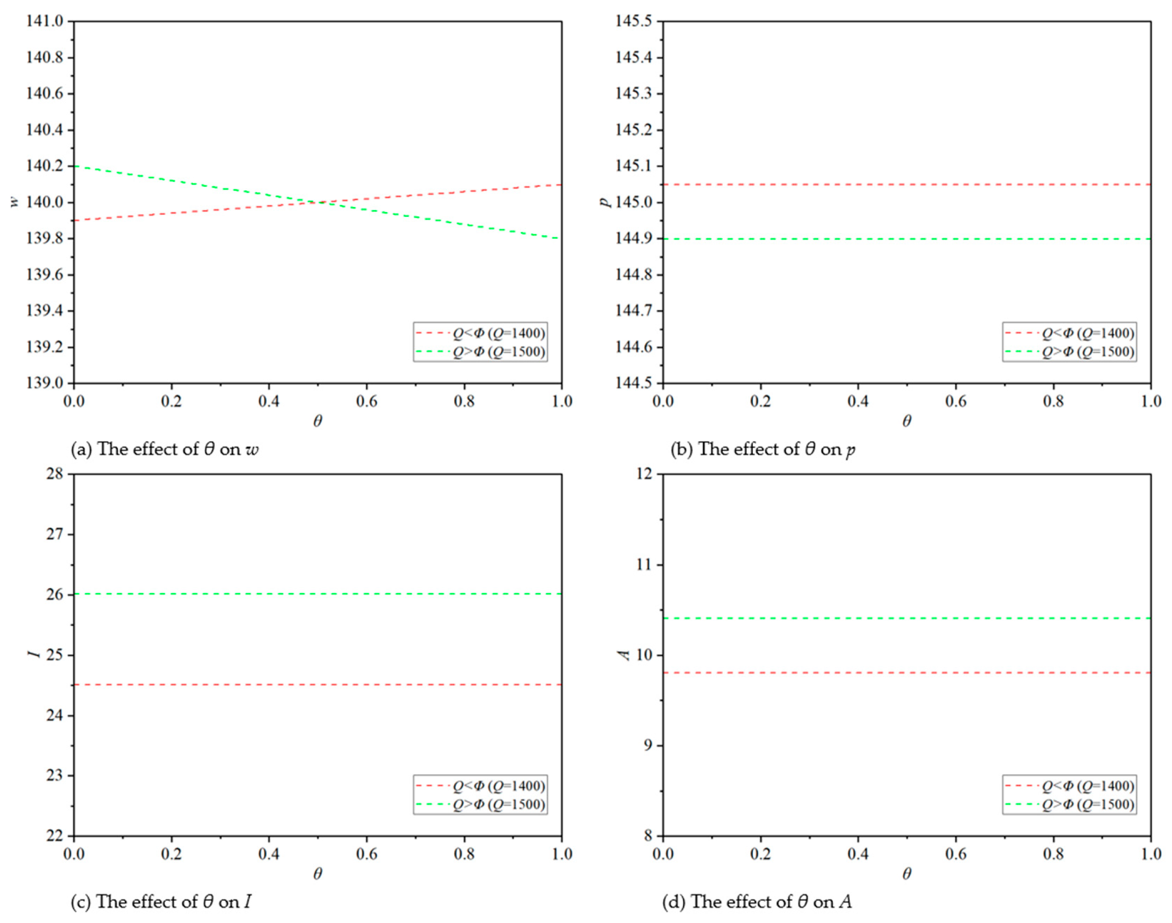
We further investigate the roles of the carbon trading cost and benefit sharing ratio. Figure 7 shows the variations in w, p, I, and A with respect to θ under the carbon trading policy in Scenario N. It can be seen that a carbon quota surplus or gap will affect the change in θ with respect to w: if there is a carbon quota surplus, the wholesale price decreases as θ increases; however, when the carbon quota is deficient, the wholesale price will increase with an increase in θ (Figure 7a). If there is a carbon quota surplus, this can be sold to generate a profit; the manufacturer and retailer share the revenue from the surplus carbon quota, and the manufacturer will lower the wholesale price. If there is a deficit in the carbon quota, the gap in the quota needs to be purchased, and the manufacturer and retailer share the cost of meeting the carbon obligation; as θ increases, the manufacturer raises the wholesale price to transfer the burden of carbon compliance, and the change in the wholesale price exactly offsets the changes in the revenue or the carbon compliance cost shared by the retailer. The retail price, endurance effort, and marketing effort are not affected by θ. When there is a surplus in the carbon quota, the wholesale price is lower and the endurance effort and marketing effort are higher than when there is a deficit in the carbon quota (Figure 7b–d). Efforts to improve the range and marketing will also be higher in a surplus than in a deficit situation (Figure 7c,d).

6. Conclusions and Managerial Implications

6.1. Conclusions

Considering the subsidy policy, we construct an eVTOL supply chain composed of a manufacturer and retailer and employ the differential game method to solve the optimal strategy, eVTOL brand goodwill, demand, and optimal profit functions of supply chain members under three decision-making models. We analyze the equilibrium results, investigate the impacts of subsidy on the decisions and profits of the manufacturer and retailer through numerical examples, and further explore the effects of carbon trading rather than subsidies. The results show the following. (1) The subsidy policy has a positive impact on the eVTOL supply chain. With a higher subsidy rate, supply chain members have more money to invest in endurance and marketing efforts to drive eVTOL and lower the wholesale and retail prices, making eVTOL more affordable. The structure of competition in the upstream market does not affect this basic conclusion. (2) The optimal endurance effort, marketing effort, eVTOL brand goodwill, and demand under the centralized decision-making model are all higher than those under the decentralized one. Within a certain feasible range, a two-way cost-sharing contract can lead to a Pareto improvement in the eVTOL supply chain, but it does not reach the level of the supply chain under centralized decision-making. (3) The optimal subsidy that maximizes social welfare is jointly influenced by α, β, c, and σ. The larger the value of α, the higher the optimal subsidy, while, the larger the values of β, c, and σ, the lower the optimal subsidy. (4) A carbon trading policy can achieve the same effect as the subsidy policy and act as an alternative: if the carbon quota is sufficiently high or the lifecycle carbon emissions significantly decrease, the endurance effort, marketing effort, eVTOL brand goodwill, and demand under the carbon trading policy will reach or even exceed those of the subsidy policy.

6.2. Managerial Implications

(1)

For policymakers, a reasonable fiscal subsidy for eVTOL should be provided to support the development of this strategic emerging industry as a new low-altitude economic model. The subsidy amount for eVTOL is high, and there is a risk of fraud; therefore, the government should improve the system design, clearly define the criteria for recognition, continuously track the implementation of enterprise R&D investment, and strengthen verification and enforcement measures. In addition, the development of eVTOL cannot always rely on government subsidies. After entering the stage of stable development, direct fiscal subsidies should be gradually replaced with a carbon trading mechanism to reduce the pressure of fiscal expenditure and use market-based measures to stimulate industrial development. It is also necessary to scientifically determine the lifecycle carbon emissions of eVTOL, reasonably allocate a carbon quota, and explore the potential for carbon trading incentives.

(2)

For enterprise managers, recommendations include understanding subsidy dividends, accelerating the R&D of endurance technology and the optimization of product performance for eVTOL, continuously improving the core competitiveness of products, and consolidating brand goodwill by relying on technology upgrading. At the same time, managers should enhance brand marketing, optimize channel management, and cultivate the low-altitude travel consumption market. Members of the automotive supply chain are encouraged to establish a mechanism of benefit and risk sharing, jointly promoting the research and development of flight technology and the supply of scenarios. They are also encouraged to actively explore and design supply chain coordination contracts that suit their own needs, in order to enhance the overall efficiency of the supply chain.

6.3. Future Research Directions

This paper contributes to the existing research, but there are limitations. Future research work can be expanded in the following aspects. Firstly, this work only considers the single-channel supply chain in which products are sold through a retailer; thus, an interesting direction would be to explore multi-channel competition. Secondly, the model assumes that parameters remain constant over an infinite period of time, without considering the impacts of random disturbances. Moreover, as eVTOL becomes more widespread, it will compete with ground vehicles such as ICEVs and NEVs; future research can explore the impacts of the development of eVTOL on such vehicles.

References

1. Zheng, M.; Zhou, T.; Du, Z. Research on the High Quality Development Path of China’s Low altitude Economy from the Perspective of New Quality Productivity. Acad. J. Bus. Manag. 2025, 7, 34–45. [Google Scholar] [CrossRef] [Scilit]
2. Shusen, W.; Gan, X. China’s low-altitude economy: Theoretical foundations, development status, and policy directions. China Econom. 2025, 20, 68–100. [Google Scholar] [CrossRef]
3. Kasliwal, A.; Furbush, N.J.; Gawron, J.H.; McBride, J.R.; Wallington, T.J.; De Kleine, R.D.; Kim, H.C.; Keoleian, G.A. A Role of flying cars in sustainable mobility. Nat. Commun. 2019, 10, 1555. [Google Scholar] [CrossRef] [Scilit] [PubMed]
4. Meng, Z.; Ji, J.; Liu, L.; Liu, S.; Sun, Z.; Xiao, Q.; Yang, Z. eVTOL aircraft for the low-altitude economy: A review of development history, core technologies, and future trends. Case Stud. Transp. Policy 2025, 22, 101629. [Google Scholar] [CrossRef] [Scilit]
5. Qian, T.; Yue, J.; Wang, C.; Li, J.; Hu, Q.; Hui, H. Urban energy and three-dimensional mobility integration for eVTOL scale-up. Appl. Energy 2026, 421, 128226. [Google Scholar] [CrossRef] [Scilit]
6. Kalakou, S.; Marques, C.; Prazeres, D.; Agouridas, V. Citizens’ attitudes towards technological innovations: The case of urban air mobility. Technol. Forecast. Soc. Change 2023, 187, 122200. [Google Scholar] [CrossRef] [Scilit]
7. Weng, C.; Pan, T.; Chen, C.; Zhong, R. Urban low-altitude air transport management: Bridging dynamic traffic control and static network equilibrium. Transp. Res. Part C Emerg. Technol. 2025, 178, 105237. [Google Scholar] [CrossRef] [Scilit]
8. Garrow, L.A.; German, B.J.; Leonard, C.E. Urban air mobility: A comprehensive review and comparative analysis with autonomous and electric ground transportation for informing future research. Transp. Res. Part C Emerg. Technol. 2021, 132, 103377. [Google Scholar] [CrossRef] [Scilit]
9. Meng, W.; Wang, Y.; Li, Y.; Huang, B. Impact of product subsidies on R&D investment for new energy vehicle firms: Considering quality preference of the early adopter group. PLoS ONE 2020, 15, e0236626. [Google Scholar] [CrossRef] [Scilit] [PubMed]
10. Wang, Y.; Zhang, X.; Cheng, T.C.E.; Wu, T.H. Choice of the co-opetition model for a new energy vehicle supply chain under government subsidies. Transp. Res. Part E Logist. Transp. Rev. 2023, 179, 103326. [Google Scholar] [CrossRef] [Scilit]
11. Li, J.X.; Li, J.Z.; Wu, Y.C. Product R&D strategy of new energy vehicle enterprises embedded with technical services under the subsidy threshold. J. Knowl. Econ. 2025, 16, 1518–1545. [Google Scholar] [CrossRef] [Scilit]
12. Biehle, T. Social sustainable urban air mobility in Europe. Sustainability 2022, 14, 9312. [Google Scholar] [CrossRef] [Scilit]
13. Bi, W.; Lyu, Y.; Shen, Y.; Ji, Y.; Du, Y. Understanding the potential of urban air mobility in alleviating rail transit oversaturation: A divertible demand driven analysis. Transp. Lett. 2026, 18, 370–391. [Google Scholar] [CrossRef] [Scilit]
14. Shen, Y.; Dong, P.; Ju, Y. Optimal government subsidy strategies for achieving urban air mobility promotion target considering infrastructure. J. Air Transp. Manag. 2026, 135, 103031. [Google Scholar] [CrossRef] [Scilit]
15. Ji, Z.; Yang, H.; Chow, J.Y. Distance-based subsidy rate design to incentivize ride-hail access to advanced air mobility hubs. J. Air Transp. Manag. 2026, 137, 103090. [Google Scholar] [CrossRef] [Scilit]
16. Dulia, E.F.; Shihab, S.A. Building public–private partnerships for advanced air mobility infrastructure using game theory. J. Air Transp. 2025, 33, 229–245. [Google Scholar] [CrossRef] [Scilit]
17. Lv, X.; Wu, D.; Wang, Y. Game-Theoretic Decision-Making for Aircraft Routing at Junctions Under Communication Jamming. In Proceedings of the 2026 38th Chinese Control and Decision Conference (CCDC); IEEE: New York, NY, USA, 2026; pp. 1774–1779. [Google Scholar] [CrossRef] [Scilit]
18. Yang, X.; Wei, P. Scalable multi-agent computational guidance with separation assurance for autonomous urban air mobility. J. Guid. Control. Dyn. 2020, 43, 1473–1486. [Google Scholar] [CrossRef] [Scilit]
19. Ding, L.; Zhu, X. The impact of the dual-credit policy on production and cooperative R&D in the automotive supply chain. Sustainability 2023, 15, 1302. [Google Scholar] [CrossRef] [Scilit]
20. Zhang, H.; Lin, J. Decision-making on price and after-sales service of new energy vehicle supply chain under different sales modes based on game theory models. J. Comb. Math. Comb. Comput. 2025, 127, 6267–6277. [Google Scholar] [CrossRef] [Scilit]
21. Gong, B.; Xia, X.; Cheng, J. Supply-chain pricing and coordination for new energy vehicles considering heterogeneity in consumers’ low carbon preference. Sustainability 2020, 12, 1306. [Google Scholar] [CrossRef] [Scilit]
22. Ma, M.; Meng, W.; Li, Y.; Huang, B. Supply chain coordination strategy for NEVs based on supplier alliance under dual-credit policy. PLoS ONE 2021, 16, e0257505. [Google Scholar] [CrossRef] [Scilit] [PubMed]
23. Yin, Y.; Liu, F. Carbon Emission Reduction and Coordination Strategies for New Energy Vehicle Closed-Loop Supply Chain under the Carbon Trading Policy. Complexity 2021, 2021, 3720373. [Google Scholar] [CrossRef] [Scilit]
24. Dulia, E.F.; Shihab, S.A. An integrated supply chain network design for advanced air mobility aircraft manufacturing using stochastic optimization. Supply Chain Anal. 2024, 8, 100083. [Google Scholar] [CrossRef] [Scilit]
25. Jin, Z.; Ng, K.K.; Zhang, C.; Wu, L.; Li, A. Integrated optimisation of strategic planning and service operations for urban air mobility systems. Transp. Res. Part A Policy Pract. 2024, 183, 104059. [Google Scholar] [CrossRef] [Scilit]
26. Wang, Z.; Lv, D.; Jia, S.; Wang, K.; Qu, X. Urban air mobility network design and operations strategy in an urban agglomeration. Transp. Res. Part E Logist. Transp. Rev. 2025, 203, 104316. [Google Scholar] [CrossRef] [Scilit]
27. Lin, S.; Zhang, G. Research on Differential Strategies Considering the Endurance and Advertising Advertising of New Energy Vehicles under the Dual Credit Policy. Chin. J. Manag. Sci. 2026, 34, 319–329. [Google Scholar] [CrossRef]
28. Liu, N.; Chen, S.; Kong, J.; Zhang, T.; Zhang, X. Differential Game Analysis in a Dual-Channel Automotive Supply Chain Under the CAFC-NEV Credits and Carbon Credit Policies. World Electr. Veh. J. 2026, 17, 128. [Google Scholar] [CrossRef] [Scilit]
29. Sun, H.; Liu, J.; Zhang, L. Differential game analysis of carbon emission reduction effect and price strategy considering government intervention and manufacturer competition. Manag. Decis. Econ. 2025, 46, 1146–1166. [Google Scholar] [CrossRef] [Scilit]
30. Zhou, Y.; Ye, X. Differential game model of joint emission reduction strategies and contract design in a dual-channel supply chain. J. Clean. Prod. 2018, 190, 592–607. [Google Scholar] [CrossRef] [Scilit]
31. He, J.; Yang, T. Differential game analysis of emission reduction and preservation in the tertiary food supply chain under different government subsidy models. Sustainability 2022, 15, 701. [Google Scholar] [CrossRef] [Scilit]
32. An, Q.; Zhu, K.; Xiong, B. Investment allocation in an adjustment-cost production technology framework for two-stage network structures. Eur. J. Oper. Res. 2024, 319, 808–819. [Google Scholar] [CrossRef] [Scilit]
33. He, L.; Yuan, B.; Bian, J.; Lai, K.K. Differential game theoretic analysis of the dynamic emission abatement in low-carbon supply chains. Ann. Oper. Res. 2023, 324, 355–393. [Google Scholar] [CrossRef] [Scilit]
34. Chen, S.; Su, J.; Wu, Y.; Zhou, F. Optimal production and subsidy rate considering dynamic consumer green perception under different government subsidy orientations. Comput. Ind. Eng. 2022, 168, 108073. [Google Scholar] [CrossRef] [Scilit]
35. Lou, Z.; Hou, F.; Lou, X.; Ma, T. Game-theoretical Models of a Two-echelon Supply Chain Involving Two Substitutable Products. J. Syst. Sci. Syst. Eng. 2021, 30, 307–320. [Google Scholar] [CrossRef] [Scilit]
36. Li, Y.; Tong, Y.; Ye, F.; Song, J. The choice of the government green subsidy scheme: Innovation subsidy vs. product subsidy. Int. J. Prod. Res. 2020, 58, 4932–4946. [Google Scholar] [CrossRef] [Scilit]
37. Zhang, Y.; Chi, Y.; Li, G.; Zhang, X. The impact of carbon tax policy on residents’ welfare of China and its heterogeneity under the carbon neutrality goal: A CGE model-based analysis. J. Clean. Prod. 2024, 434, 140442. [Google Scholar] [CrossRef] [Scilit]
38. Liu, M.; Hao, H.; Geng, Y.; Dou, H.; Sun, X.; Bai, F.; Qu, X.; Wang, K.; Liu, Z.W.; Zhao, F.Q. Adopting Electric Vertical Takeoff and Landing Aircraft for Green Transport Transformation. Fundam. Res. 2026, 6, 2621–2633. [Google Scholar] [CrossRef] [Scilit] [PubMed]
Figure 1. The feasible region of φ1 and φ2 under the cost-sharing contract.
Systems 14 01079 g001
Figure 2. The trajectory of eVTOL brand goodwill.
Systems 14 01079 g002
Figure 3. The variations in p, I, A, and D with respect to s in Scenarios C, N, and S.
Systems 14 01079 g003
Figure 4. The variations in Jmr, Jm, and Jr with respect to s in Scenarios C, N, and S.
Systems 14 01079 g004
Figure 5. The variations in I, A, and D with respect to Q under the government subsidy and carbon trading policy in Scenarios C and N.
Systems 14 01079 g005
Figure 6. The variations in Jmr, Jm, and Jr with respect to Q under the government subsidy and carbon trading policy in Scenarios C and N.
Systems 14 01079 g006
Figure 7. The variations in w, p, I, and A with respect to θ under the carbon trading policy in Scenario N.
Systems 14 01079 g007