The Interplay of Financing and Trade-In Implementation Under Agency Selling

Highlights

Please indicate how your work links to systems science via your contributions to systems practice, theory, and/or methodology.

• Treating financing and trade-in implementation as one system corrects the distortions of analyzing either dimension alone.
• Firms and policymakers should weigh financing and trade-in decisions jointly, not in isolation, since the two interact.

What are the main findings and/or the implications of the main findings?

• In contrast with the no-financing trade-in supply chain, financing reshapes the manufacturer’s and the platform’s preferred trade-in implementer.
• Who lends does more than set the rate; it restructures the chain and induces substantive changes in decision making.

Abstract

A capital-constrained manufacturer sells a durable product to replacement consumers (consumers with a used product) and primary consumers (consumers without one) through a retail platform under agency selling, financing production from either the platform or a bank, with the trade-in program implemented by either the manufacturer or the platform. Four supply chain models are formulated and solved. Comparing the equilibrium decisions and demands, the rankings across the two financing channels are generally cost-dependent, whereas several comparisons across the two trade-in implementers are stable or structurally pinned down. Introducing financing reshapes the trade-in preferences of the manufacturer and the platform relative to agency selling without financing. In the reported numerical comparisons, the manufacturer largely prefers platform financing, and the bank always prefers platform implementation; consumers prefer platform financing when the manufacturer implements the trade-in and manufacturer implementation under platform financing. Three extensions respectively confirm the effects of financing, examine how the government should set the trade-in subsidy, and assess the robustness of the key findings when the manufacturer has positive initial capital.

1. Introduction

A growing number of platforms, such as JD.com, Tmall, and Amazon, are opening their online marketplaces to manufacturers or third-party sellers, letting them sell directly to consumers under agency selling in exchange for a commission on each sale. Most of these firms are small and medium-sized businesses: on Amazon, for instance, about 73% of third-party sellers employ only one to five people, and another 10% employ five to ten [1]. Firms of this size often lack working capital and must rely on short-term financing to cover production and procurement before sales revenue comes in [2].

Such financing has traditionally come from banks. Platforms now also finance manufacturers, either directly or in cooperation with financial institutions. JD.com lends to its merchants through its own supply chain finance program, Jingbaobei; Alibaba provides financing to its Taobao and Tmall sellers through MYbank, the online bank of its fintech affiliate Ant Group; and Amazon arranges credit for its sellers through partner lenders under Amazon Lending. Following Xu et al. [3], we refer to both direct platform lending and platform-led cooperative lending as platform financing. When an external financial institution participates in such an arrangement, we treat the platform and the financial institution as an integrated financing entity, so the entity internalizes both commission revenue and lending returns. By contrast, under bank financing, an independent bank makes the lending decision without internalizing the platform’s commission revenue. A capital-constrained manufacturer can therefore finance its production through either platform financing or bank financing.

Beyond financing, these manufacturers face an increasingly saturated product market. Advances in technology have made many products, e.g., consumer electronics, ever more durable, so more and more consumers in the market already hold a used product. Trade-in programs, in which a consumer returns a used product for a rebate toward a new purchase, convert this stock of used products into replacement demand, and have therefore gained increasing favor among manufacturers and retailers [4]. Competitive pressure has extended the practice to the online marketplaces as well: JD.com, Amazon, and Taobao now offer trade-in services to consumers who purchase third-party products on their sites.

Trade-in implementation and financing have thus become a coupled pair of problems in the operation of platform supply chains. Policy makes the coupling explicit: China’s 2026 Government Work Report arranges RMB 250 billion of ultra-long-term special treasury bonds to subsidize consumer goods trade-ins, alongside a RMB 100 billion fiscal–financial fund that supports enterprise financing through loan interest subsidies, financing guarantees, and risk compensation (https://www.ndrc.gov.cn/xwdt/ztzl/tddgmsbgxhxfpyjhx/gzdt/202603/t20260316_1404171.html (accessed on 26 June 2026)). A more concrete example comes from Tmall. Hangzhou Songxing Technology Co., Ltd. (Hangzhou, China), an Apple-authorized reseller operating a third-party store on Tmall, received a dedicated credit line from MYbank based on its transaction data (https://finance.sina.com.cn/wm/2025-08-18/doc-infmmmiz8330329.shtml (accessed on 8 August 2026)). Tmall also offers trade-in services for this product category. The policy initiative and this firm-level case together underscore the need to treat the two issues within a unified decision framework. The literature, however, has typically studied the two dimensions separately: one stream examines trade-in programs, e.g., [5,6,7], and another examines financing choices, e.g., [1,3,8]. To address this gap, we investigate how the two dimensions interact. Specifically, we consider a capital-constrained manufacturer that sells a new durable product through an online retail platform under agency selling. The manufacturer can raise funds from either the platform or a bank, and the trade-in program can be implemented by either the manufacturer or the platform. Against this backdrop, we address the following questions.

• What are the equilibrium decisions—the interest rate, the new-product price, and the trade-in rebate—in each scenario?
• How do the financing source (platform versus bank) and the trade-in implementer (manufacturer versus platform) interact to shape these decisions and the resulting demand?
• From the perspectives of the manufacturer, the platform, the bank, and consumers, which trade-in implementer and which financing channel are preferred?

To answer these questions, we build four game-theoretic models, denoted $MP$, $MB$, $PP$, and $PB$ by the trade-in implementer (the manufacturer M or the platform P) and the financing source (the platform P or a bank B), in which a fraction of consumers own a used product while the others do not, the platform charges a fixed commission, and the manufacturer borrows to finance its production and procurement. We also examine three extensions: a no-financing benchmark, a government trade-in subsidy, and the manufacturer’s positive initial capital. Solving these models and comparing the equilibria across scenarios, we obtain the following main findings.

First, the financing channel and the trade-in implementer shape the equilibrium decisions in different ways. A platform-implemented trade-in raises the equilibrium interest rate relative to a manufacturer-implemented one, whereas whether platform or bank financing yields the higher rate depends on the production cost. The two dimensions’ effects on prices and demand are likewise largely cost-dependent, with two regularities under platform financing: a platform-implemented trade-in consistently pays a larger rebate, and total new-product demand is the same regardless of which party implements the trade-in.

Second, the financing channel reshapes who prefers to implement the trade-in. Under platform financing, both the manufacturer and the platform prefer to implement the program themselves, whereas under bank financing their preferences become mixed.

Third, we compare the preferences of the parties across the two dimensions. Under the numerical settings, the bank consistently prefers the platform to implement the trade-in; the manufacturer’s preferred financing channel depends on the residual value of used products and the production cost, but, in most cases, it favors platform financing; consumers prefer platform financing when the manufacturer implements the trade-in and prefer the manufacturer to implement the trade-in under platform financing.

Fourth, the no-financing extension confirms the effects of financing. The government-subsidy extension shows that the welfare-maximizing subsidy rate depends on both the supply chain structure and the production cost. The positive-initial-capital extension shows that positive initial capital does not substantially change this paper’s main findings.

The remainder of this paper is organized as follows. Section 2 reviews the related literature. Section 3 describes the problem and assumptions. Section 4 presents the four scenarios and characterizes the equilibrium decisions. Section 5 compares the scenarios along the financing and implementation dimensions. Section 6 presents the extensions. Section 7 concludes and outlines directions for future research. All proofs are collected in Appendix A.

2. Literature Review

This paper relates to two research streams: (i) trade-in programs for durable goods and (ii) financing for capital-constrained supply chains. We review these streams and position our contribution accordingly.

2.1. Trade-In Programs for Durable Goods

Within the scope of durable-goods operations, trade-in programs have been extensively studied; the literature falls into two substreams, one on the pricing of the program and the other on the choice of its implementer.

The majority of the studies in this stream focus on the pricing of the program and the associated strategy choices. For durable goods sold in a highly saturated market, Ray et al. [9] compare three pricing strategies: a uniform price for all consumers, prices differentiated by whether a consumer owns a used product, and prices further conditioned on the age of the used product. Yin and Tang [10] ask when a trade-in program should charge an up-front participation fee when consumers are uncertain about their valuation of the new product. Yin et al. [11] extend the pricing problem to two successive product generations whose incremental value is uncertain before introduction. Cao et al. [12] study how a retail platform implements its trade-in program and whether the program should cover the third-party stores it hosts. In a multi-period framework, Xiao et al. [13] evaluate the performance of fully dynamic pricing against semi-dynamic pricing in which the new-product price is fixed and only the rebate adjusts. Cao and Choi [14] account for consumer returns and study the associated trade-in refund policy. Dong et al. [15] examine the trade-in strategies of two competing manufacturers when consumers incur switching costs. Tang et al. [7] examine how the government should design its subsidy scheme when a single firm implements the trade-in.

Because a trade-in naturally serves as a collection channel for used products, a growing body of work examines its interaction with used-product sales. Rao et al. [16] show that trade-ins can mitigate the lemons problem in used-goods markets. Agrawal et al. [17] study the trade-in rebate both as a price-discrimination device and as a means of collecting used products for remanufacturing. Zhao et al. [18] analyze how a manufacturer can deploy a trade-in program to compete with a third-party remanufacturer. Turning to used-product resale, Vedantam et al. [19] ask whether a manufacturer should run a trade-in program or open its own peer-to-peer marketplace; Hu et al. [20] examine when a manufacturer operating a trade-in program should refurbish the returned products; and Bai et al. [21] study the manufacturer’s implementation modes in the presence of a resale platform, distinguished by whether the rebate is paid in cash. Li et al. [22] consider hybrid manufacturing and remanufacturing with a trade-in program under a carbon tax. Hu et al. [23] incorporate time-varying customer choice behavior and changing secondary-market recycling prices into the pricing problem. Hu et al. [24] derive the pricing and resale strategies when a secondary market and a trade-in program coexist, and Srivastava et al. [25] identify when a manufacturer should cooperate with a third-party collection platform to implement the trade-in.

The other substream examines the choice of the trade-in implementer, which is closely related to our work. In a reselling supply chain, Tang et al. [4] study whether the manufacturer or the retailer should implement the trade-in program. Taking the resale of the collected products into account, Li et al. [26] ask whether the retailer or a collection platform should implement it. Wang et al. [6] compare the reselling and agency modes and investigate who should implement the program, the manufacturer or the platform, under each mode. Considering consumers’ quality preferences, Ma et al. [27] study the same choice between the manufacturer and the retail platform, and Zheng et al. [28] further examine it when the collected used products can be resold.

Although this stream has studied trade-in programs in depth, covering their pricing, their interplay with the used-product market, and who should implement them, it assumes a well-funded manufacturer. These studies do not consider a capital-constrained manufacturer that must finance production, nor who should provide that financing.

2.2. Financing for Capital-Constrained Supply Chains

Classic supply-chain finance contrasts an external bank with an upstream lender. Buzacott and Zhang [29] first incorporate asset-based financing into production decisions, showing that a firm’s inventory decisions and its access to asset-based credit are inseparable. Kouvelis and Zhao [30] characterize the optimal trade-credit contract for a news vendor that can borrow from its supplier or a bank. Kouvelis and Zhao [31] further show that the firms’ credit ratings determine who should finance the chain’s inventory and at what rates, with a well-rated supplier offering interest-free trade credit and a poorly rated one setting a positive rate that pushes the retailer to combine trade credit with bank loans. Du et al. [32] examine how the manufacturer’s introduction of a direct channel interacts with the retailer’s choice between trade credit and bank credit.

With the development of the online economy, e-commerce platforms have emerged as a new source of financing and have drawn increasing research attention. Considering a manufacturer that sells through a traditional retailer and, under agency selling, an online platform, Zhen et al. [33] study the manufacturer’s financing choice among the retailer, the platform, and a bank. Yang et al. [34] identify the conditions under which a third-party retailer borrowing from the bank and the platform simultaneously achieves a Pareto improvement for the supply chain. Wang et al. [35] show how farmers’ social responsibility shapes their financing-channel choice between a bank and the platform. Mandal et al. [1] examine the bank-versus-platform financing choice of two competing sellers hosted on a platform. When carbon permits can serve as pledged assets, Xu et al. [3] study how the seller’s remanufacturing and carbon-abatement decisions interact with its financing choice between the platform and the bank. Lu et al. [8] investigate how the platform’s digital empowerment affects farmers’ loan choice between the platform and a bank. Liu et al. [36] study a supplier’s online selling-mode choice between agency and reselling when the platform offers financing, with the supplier also holding an offline reselling channel. Under exogenous and endogenous default risks, Huang et al. [2] analyze how a third-party seller should choose between trade credit from its supplier and platform financing. When third-party sellers trade through a platform, Hu et al. [37] examine the interplay between information sharing and financing services on the retail platform. For a low-carbon supply chain with an upstream supplier and two capital-constrained retailers, Zhang et al. [38] evaluate how supplier financing and hybrid financing affect the chain’s performance. Jiang et al. [39] study the financing choice of a retailer hosted on a platform between its upstream supplier and the platform. Liao et al. [40] examine how the sharing of farmers’ technology-investment costs affects their loan choice between the platform and a bank. Wang et al. [41] study how channel competition and consumers’ low-carbon preference drive the financing-channel choice of a capital-constrained manufacturer or retailer. Considering consumer-oriented advance-selling financing, Wang et al. [42] compare a retailer’s three financing options: trade credit alone, advance selling alone, or the two combined.

In recent years, governments have begun to intervene with subsidy and interest-subsidy policies to stimulate the economy, and a group of studies has accordingly turned to financing decisions under government subsidies. Luo et al. [43] study how the government should choose between risk compensation and guarantee-fee reduction when facing capital-constrained small and medium-sized businesses and a profit-maximizing guarantee company. When two competing farmers borrow from a bank, Yi et al. [44] examine the government’s choice between an interest subsidy and a direct subsidy. In an industrial-symbiosis setting with supply–demand mismatch, Cao et al. [45] compare purchase-order financing, factoring, and buyer direct financing in terms of supply-chain performance and further analyze how an environmental tax and a recycling subsidy alter the value of each mode. When the manufacturer raises green equity financing, Zhou et al. [46] compare three government subsidy targets, namely, the manufacturer, the retailer, and consumers.

These studies examine financing for production, inventory, or green investment, but do not consider how the source of production financing interacts with who implements the trade-in program.

Differing from the existing literature, we simultaneously consider the trade-in implementation responsibility and the financing responsibility of a capital-constrained manufacturer under agency selling. The manufacturer sells a durable product through a retail platform; it finances production from either the platform or a bank, while the trade-in program is implemented by either the manufacturer or the platform. Financing makes the interest rate an endogenous decision and links the lender’s rate-setting problem to the trade-in implementer’s rebate decision. The trade-in implementer determines who bears the rebate cost, which changes the manufacturer’s operating burden and, hence, the lender’s optimal rate; the financing source determines whether the platform internalizes the lending return from trade-in-induced sales together with its commission or whether that return accrues to an external bank. This feedback between rebate cost exposure and financing return internalization changes equilibrium rates, prices, rebates, and demand and thereby reshapes supply chain members’ preferences over the trade-in implementer.

Table 1. Positioning of this paper relative to representative studies.

Study	Trade-In	Implementer	Capital Constraint	Financing Source
Tang et al. [4]	✓	M or R
Wang et al. [6]	✓	M or P
Ma et al. [27]	✓	M or P
Zheng et al. [28]	✓	M or P
Mandal et al. [1]			✓	P or B
Xu et al. [3]			✓	P or B
Lu et al. [8]			✓	P or B
Zhen et al. [33]			✓	P or B
Yang et al. [34]			✓	P and B
Wang et al. [35]			✓	P or B
Liao et al. [40]			✓	P or B
This paper	✓	M or P	✓	P or B

Note: A checkmark indicates that the study considers the corresponding dimension.

summarizes this positioning relative to representative studies; there, M, R, P, and B denote the manufacturer, the retailer, the platform, and the bank, respectively.

3. Problem Description and Assumptions

3.1. Problem Description

We consider a platform-based supply chain in which a capital-constrained manufacturer sells a durable product to consumers through a retail platform under agency selling. Under this mode, the manufacturer sets the new-product price, $p_n$, while the platform charges a commission on the sales revenue at an exogenous rate $\varphi$ ($0<\varphi <1$). There are two types of consumers in the market: a fraction $\alpha$ ($0<\alpha <1$) own a used product and are referred to as replacement consumers ($C_R$), whereas the remaining fraction $1-\alpha$ do not own a used product and are referred to as primary consumers ($C_N$), as in [9]. The manufacturer lacks capital and needs financing in order to produce. We consider two financing channels, the platform and a bank; the manufacturer borrows from one of them and repays the loan at an interest rate r once demand is realized. For tractability, we assume that the manufacturer has zero initial capital and funds its entire unit production cost c externally, a common assumption in the supply-chain finance literature (e.g., [1,3,44]). Section 6.3 relaxes this assumption. To encourage replacement consumers to replace their used product with the new one, we further allow a trade-in program, implemented either by the manufacturer or by the platform, that pays a replacement consumer a rebate $p_t$ for the used product upon repurchase. Here, trade-in implementation refers only to setting and paying the rebate; we abstract from the costs of collecting, inspecting, transporting, and refurbishing returned used products (see also [4,5,20]).

As introduced in Section 1, the trade-in implementer and the financing source jointly define four scenarios: $MP$, $MB$, $PP$, and $PB$. The platform may thus play up to two roles—financing production and implementing the trade-in program—in addition to operating the marketplace. For analytical convenience, we assume that collected used products have zero net recovery value, as in [17]. This assumption applies to the low-value electronics products, which are typically dismantled for material recovery and generate limited net recovery value. 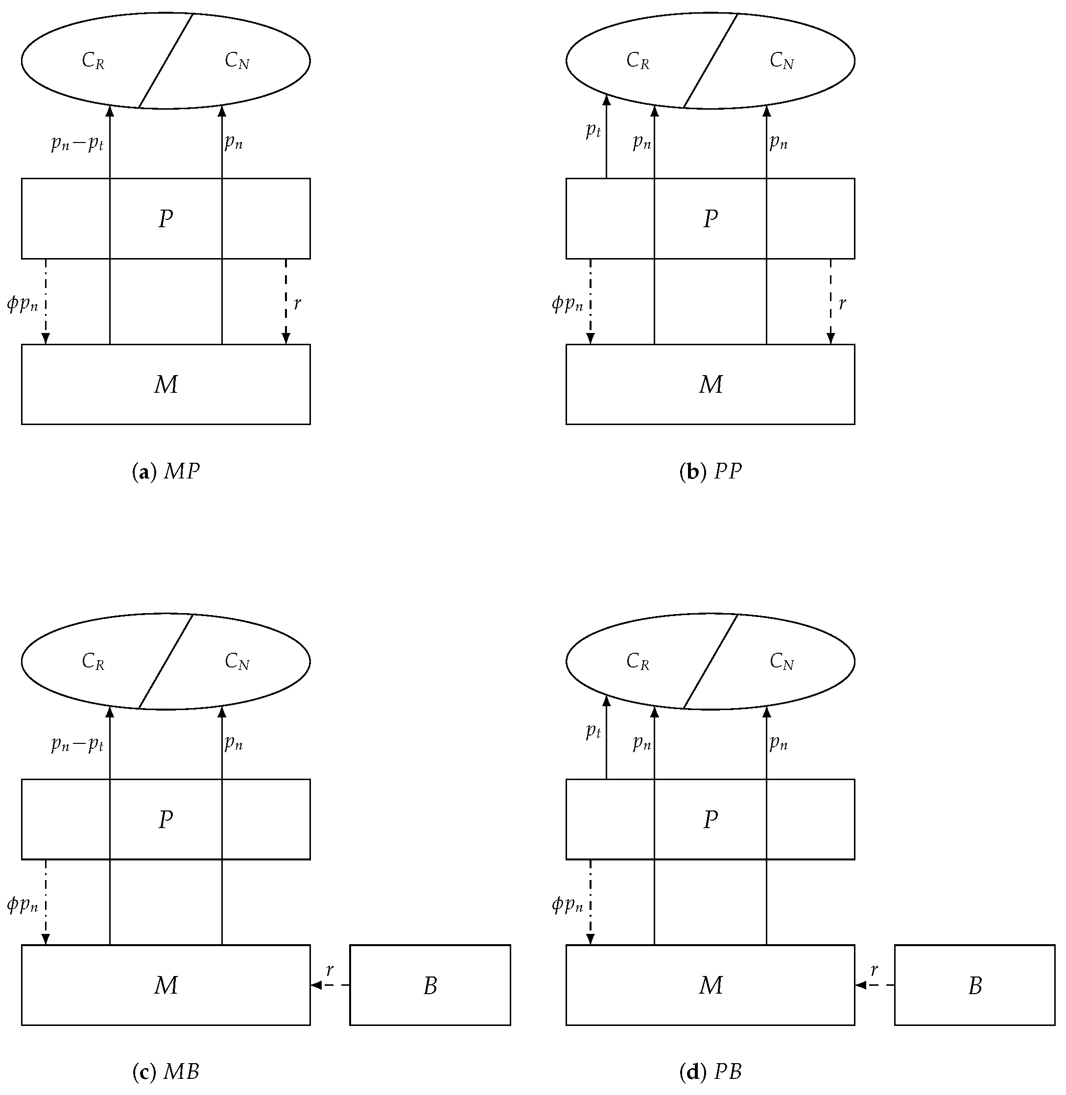These four configurations form a $2\times 2$ design that allows us to study the interplay of financing and trade-in modes under agency selling. The supply chain structure of each scenario is depicted in Figure 1, and all notation is summarized in

Table 2. Notation.

Notation	Description
c	Unit production cost, $0<c<1$
$\varphi$	Platform commission rate, $0<\varphi <1$
r	Financing interest rate
$\alpha$	Fraction of replacement consumers, $0<\alpha <1$
$\delta$	Residual value of the used product, $0<\delta <1$
$p_n$	Price of the new product
$p_t$	Trade-in rebate
$q_{nr}$	Demand from replacement consumers ($C_R$)
$q_{nn}$	Demand from primary consumers ($C_N$)
$q_n$	Total demand for the new product, $q_n=q_{nr}+q_{nn}$
i	Scenario index, $i\in \{MP,MB,PP,PB\}$, combining the trade-in implementer (manufacturer M or platform P) with the financing source (platform P or bank B)
${\Pi }_m^i,{\Pi }_p^i,{\Pi }_b^i$	Profit of the manufacturer, platform, and bank in scenario i

.

Throughout, we assume that the bank and the platform act as the leaders of the supply chain: they decide first, and the manufacturer decides afterward. This assumption is consistent with [1,3,28] and with practice, in which the manufacturer needs to know the interest rate before it produces, while firms that rely on such financing are typically small and medium-sized enterprises in a weaker decision position relative to large platforms and therefore tend to act as followers in operational decisions. The detailed decision sequence is as follows. In the first stage, the lender sets the interest rate r and, if the platform implements the trade-in program, the platform sets the rebate $p_t$. In the second stage, the manufacturer sets the new-product price $p_n$ and, if it implements the trade-in program, the rebate $p_t$.

To rule out degenerate outcomes, we focus throughout on the interior parameter region in which, in each scenario, the financing rate r, the new-product price $p_n$, the rebate $p_t$, and the effective price $p_n-p_t$ are positive; the manufacturer’s per-unit margin is positive on every consumer segment it serves, namely, $(1-\varphi )p_n-(1+r)c>0$ on a primary unit in every scenario and, when the manufacturer funds the rebate (scenarios $MP$ and $MB$), $(1-\varphi )p_n-p_t-(1+r)c>0$ on a replacement unit; the segment demands $q_{nn}$ and $q_{nr}$ are positive, so that both segments are served.

3.2. Demand

We assume that each consumer’s valuation of the new product, $\theta$, is uniformly distributed on $[0,1]$. This assumption is widely adopted in operations management models to represent heterogeneous willingness to pay while retaining a tractable aggregate demand function (e.g., [4,5,21,25,28]). The market size is normalized to one. For a replacement consumer, the used product still carries a residual value of $\delta \theta$, where $\delta$ ($0<\delta <1$) is the residual-value factor and $1-\delta$ captures its depreciation, referring to [21,26,47].

A replacement consumer obtains utility $U_{nr}=\theta -p_n+p_t$ from purchasing a new product, whereas keeping the used product yields $U_{ku}=\delta \theta$; the purchasing condition $U_{nr}\ge U_{ku}$ yields $q_{nr}^i=\alpha \left(1-{\displaystyle \frac{p_n-p_t}{1-\delta }}\right)$. A primary consumer obtains utility $U_{nn}=\theta -p_n$ from buying the new product and the purchasing condition $U_{nn}\ge 0$ yields $q_{nn}^i=(1-\alpha )(1-p_n)$ for $i\in \{MP,MB,PP,PB\}$. This deterministic demand specification abstracts from random demand shocks. It is applicable when demand is relatively stable over the decision horizon or can be estimated with reasonable accuracy from historical sales data. Closely related utility-based demand specifications are widely used in the trade-in literature (e.g., [12,19,24]).

4. Models and Optimal Decisions

This section constructs the model for each scenario and presents the optimal decisions of the supply chain members.

4.1. Scenario $MP$

In scenario $MP$, the manufacturer implements the trade-in program and chooses platform financing. The platform first sets the interest rate r, and the manufacturer then jointly sets the new-product price $p_n$ and the rebate $p_t$. The manufacturer and the platform solve

$$\underset{p_n,p_t}{\max }{\Pi }_m^{MP}=(1-\varphi )p_n{q}_n-p_t{q}_{nr}-(1+r)c{q}_n,$$

(1)

and

$$\underset{r}{\max }{\Pi }_p^{MP}=\varphi p_n{q}_n+rc{q}_n,$$

(2)

respectively.

Theorem 1.

In scenario $MP$, a unique equilibrium exists when $0<\varphi <\overline{\varphi }$. The interest rate is $r^{MP\ast }={\displaystyle \frac{A^{MP}}{4c(1-\alpha )(1-\delta )(2-\varphi )(1-(1-\alpha \left)\delta \right)}}$, the new-product price is $p_n^{MP\ast }={\displaystyle \frac{B^{MP}}{4(1-\alpha )(1-\delta )(2-\varphi )(1-(1-\alpha \left)\delta \right)}}$, and the trade-in rebate is $p_t^{MP\ast }={\displaystyle \frac{C^{MP}}{4(1-\alpha )(2-\varphi )(1-\delta )}}$, where the threshold is $\overline{\varphi }={\displaystyle \frac{2}{\alpha }}(\sqrt{(1-\alpha )(1-\delta )(1-(1-\alpha \left)\delta \right)}-(1-\alpha )(1-\delta ))$. The interior condition requires that $\max \{0,{\underline{c}}_t^{MP}\}<c<\min \{1,{\overline{c}}_r^{MP},{\overline{c}}_{nr}^{MP}\}$. The aggregates $A^{MP}$, $B^{MP}$, $C^{MP}$ and the cost thresholds are given in Appendix B.

In Theorem 1, the restriction on $\varphi$ indicates that the commission rate cannot be too high. This is consistent with both practice and the literature: on JD’s open platform the transaction fee is about 0.6% and the operation-support service fee ranges from 0 to 10% https://learn-jdm.jd.com/knowledge/rule/detail?ruleId=1334355128174493696 (accessed on 20 June 2026), while Mandal et al. [1] assume $\varphi <{\displaystyle \frac{1}{2}}$. The lower bound in the interior condition ensures a positive trade-in rebate, whereas ${\overline{c}}_r^{MP}$ and ${\overline{c}}_{nr}^{MP}$ ensure a positive interest rate and positive replacement demand, respectively.

4.2. Scenario $MB$

In scenario $MB$, the manufacturer implements the trade-in program and chooses bank financing. The bank first sets the interest rate r and the manufacturer then jointly sets the new-product price $p_n$ and the rebate $p_t$, while the platform only collects commission. The manufacturer and the bank solve

$$\underset{p_n,p_t}{\max }{\Pi }_m^{MB}=(1-\varphi )p_n{q}_n-p_t{q}_{nr}-(1+r)c{q}_n,$$

(3)

and

$$\underset{r}{\max }{\Pi }_b^{MB}=rc{q}_n,$$

(4)

respectively.

Theorem 2.

In scenario $MB$, a unique equilibrium exists when $\varphi <\overline{\varphi }$, with $\overline{\varphi }$ as in Theorem 1: the interest rate is $r^{MB\ast }={\displaystyle \frac{2(1-\delta )-\varphi (2-(2-\alpha \left)\delta \right)-2c(1-(1-\alpha \left)\delta \right)}{4c(1-(1-\alpha \left)\delta \right)}}$, the new-product price is $p_n^{MB\ast }={\displaystyle \frac{A^{MB}}{4(1-(1-\alpha )\delta )(4(1-\alpha )(1-\delta )(1-\varphi )-\alpha {\varphi }^2)}}$, and the rebate is $p_t^{MB\ast }={\displaystyle \frac{B^{MB}}{4(4(1-\alpha )(1-\delta )(1-\varphi )-\alpha {\varphi }^2)}}$. The interior condition requires that $\max \{0,{\underline{c}}_t^{MB},{\underline{c}}_e^{MB}\}<c<\min \{1,{\overline{c}}_{nr}^{MB}\}$. The aggregates $A^{MB}$, $B^{MB}$ and the cost thresholds are given in Appendix B.

The lower bounds in the interior condition ensure a positive rebate and a positive effective price for replacement consumers, whereas ${\overline{c}}_{nr}^{MB}$ ensures positive replacement demand.

4.3. Scenario $PP$

In scenario $PP$, the platform implements the trade-in program and the manufacturer chooses platform financing. The platform first jointly sets the interest rate r and the rebate $p_t$ and the manufacturer then sets the new-product price $p_n$. The manufacturer and the platform solve

$$\underset{p_n}{\max }{\Pi }_m^{PP}=(1-\varphi )p_n{q}_n-(1+r)c{q}_n,$$

(5)

and

$$\underset{r,p_t}{\max }{\Pi }_p^{PP}=\varphi p_n{q}_n+rc{q}_n-p_t{q}_{nr},$$

(6)

respectively.

Theorem 3.

In scenario $PP$, there exists a unique equilibrium: the interest rate is $r^{PP\ast }={\displaystyle \frac{A^{PP}}{2c(2-\varphi )(1-(1-\alpha \left)\delta \right)}}$, the new-product price is $p_n^{PP\ast }={\displaystyle \frac{B^{PP}}{2(2-\varphi )(1-(1-\alpha \left)\delta \right)}}$, and the rebate is $p_t^{PP\ast }={\displaystyle \frac{\delta }{2}}$. The interior condition requires that $0<c<\min \{{\overline{c}}_r^{PP},{\overline{c}}_{nr}^{PP}\}$. The aggregates $A^{PP}$, $B^{PP}$ and the cost thresholds are given in Appendix B.

The upper bounds ${\overline{c}}_r^{PP}$ and ${\overline{c}}_{nr}^{PP}$ ensure a positive interest rate and positive replacement demand, respectively.

4.4. Scenario $PB$

In scenario $PB$, the platform implements the trade-in program and the manufacturer chooses bank financing. The bank sets the interest rate r and the platform sets the rebate $p_t$ simultaneously in the first stage; the manufacturer then sets the new-product price $p_n$. The manufacturer, the bank, and the platform solve

$$\underset{p_n}{\max }{\Pi }_m^{PB}=(1-\varphi )p_n{q}_n-(1+r)c{q}_n,$$

(7)

$$\underset{r}{\max }{\Pi }_b^{PB}=rc{q}_n,$$

(8)

and

$$\underset{p_t}{\max }{\Pi }_p^{PB}=\varphi p_n{q}_n-p_t{q}_{nr},$$

(9)

respectively.

Theorem 4.

In scenario $PB$, there exists a unique equilibrium: the interest rate is $r^{PB\ast }={\displaystyle \frac{A^{PB}}{c(1-(1-\alpha )\delta )H^{PB}}}$, the new-product price is $p_n^{PB\ast }={\displaystyle \frac{B^{PB}}{2(1-\varphi )(1-(1-\alpha )\delta )H^{PB}}}$, and the rebate is $p_t^{PB\ast }={\displaystyle \frac{C^{PB}}{(1-\varphi )H^{PB}}}$. The interior condition requires that $\max \{0,{\underline{c}}_t^{PB},{\underline{c}}_e^{PB}\}<c<\min \{1,{\overline{c}}_{nr}^{PB},{\overline{c}}_{nn}^{PB}\}$. The aggregates $A^{PB}$, $B^{PB}$, $C^{PB}$, $H^{PB}$ and the cost thresholds are given in Appendix B.

The lower bounds in the interior condition ensure a positive rebate and a positive effective price for replacement consumers, whereas ${\overline{c}}_{nr}^{PB}$ and ${\overline{c}}_{nn}^{PB}$ ensure positive replacement and primary demand, respectively.

5. Comparative Analysis

In this section, we compare the four scenarios along two dimensions: fixing the trade-in implementer while switching the financing source and fixing the financing source while varying the trade-in implementer. All comparisons are made over the intersection of the parameter regions satisfying the relevant scenario-specific interior conditions and, where applicable, the concavity condition on $\varphi$. For each analytical result, we provide both a proof and numerical evidence to ensure that it is realized within the feasible region.

5.1. Interest Rate

Proposition 1.

(1) Under a fixed trade-in implementer, platform versus bank financing:

• (i) under a manufacturer-implemented trade-in, $r^{MP\ast }\ge r^{MB\ast }$ if $c\le c_1^I$ and $r^{MP\ast }<r^{MB\ast }$ otherwise;
• (ii) under a platform-implemented trade-in, $r^{PP\ast }\ge r^{PB\ast }$ if $c\le c_2^I$ and $r^{PP\ast }<r^{PB\ast }$ otherwise.
• (2) Under a fixed financing source, manufacturer versus platform trade-in:
• (i) under platform financing, $r^{PP\ast }>r^{MP\ast }$;
• (ii) under bank financing, $r^{PB\ast }>r^{MB\ast }$.
• The thresholds $c_1^I$ and $c_2^I$ are given in Appendix B.

Proposition 1(1) fixes the trade-in implementer and compares the interest rate under platform versus bank financing. The ranking of the two rates is cost-dependent. This finding differs from that of Mandal et al. [1], who study two competing third-party sellers that simultaneously choose between bank and platform financing. When both sellers choose the same financing source, they find that the bank always charges a higher interest rate because it earns only interest, whereas the platform earns both interest and commission revenue and lowers its rate to stimulate demand. Introducing the trade-in program changes this cost structure by adding a rebate cost borne by the trade-in implementer. The resulting interaction between the platform’s commission incentive and its channel power makes the rate ordering depend on production cost. When the cost is high, new-product demand is fragile, so the platform holds its rate below the bank’s to protect the commission it would lose if a high rate suppressed demand. When the cost is low, demand is ample and the commission base is secure even at a high rate, so the platform exercises its power and charges a rate above the bank’s.

Proposition 1(2) fixes the lender and compares the interest rate under a manufacturer- versus platform-implemented trade-in. Under either lender, a platform-implemented trade-in carries the higher rate, and the reason for this is related to who bears the rebate. When the manufacturer implements the trade-in (scenarios $MP$ and $MB$), it funds the rebate on top of repaying the production loan, so the lender cuts the rate to avoid overburdening the manufacturer and suppressing demand. When the platform implements it (scenarios $PP$ and $PB$), the manufacturer is shielded from the rebate and the lender charges more. The party that bears the trade-in cost thus pulls the financing rate down.

5.2. Prices and Demands

In this section, we compare the new-product price first, the rebate next, and the total demand they induce last.

5.2.1. New-Product Price

Proposition 2.

(1) Under a fixed trade-in implementer, platform versus bank financing:

• (i) under a manufacturer-implemented trade-in, $p_n^{MP\ast }\ge p_n^{MB\ast }$ if $c\le c_1^I$ and $p_n^{MP\ast }<p_n^{MB\ast }$ otherwise;
• (ii) under a platform-implemented trade-in, $p_n^{PP\ast }\ge p_n^{PB\ast }$ if $c\le c_1^P$ and $p_n^{PP\ast }<p_n^{PB\ast }$ otherwise.
• (2) Under platform financing, $p_n^{MP\ast }<p_n^{PP\ast }$.
• The threshold $c_1^P$ is given in Appendix B.

Proposition 2(1) fixes the trade-in implementer and compares the new-product price under platform versus bank financing. As with the rate, the ranking is cost-dependent. Financing-cost pass-through contributes to this cost dependence: because the manufacturer funds production with the loan, a higher rate raises its marginal cost and the price it sets.

Proposition 2(2) fixes platform financing and compares the new-product price under a manufacturer- versus platform-implemented trade-in. The platform-implemented program carries the higher price. The rationale is as follows. When the manufacturer implements the trade-in, it sets the new-product price and the rebate jointly and coordinates the two, holding the price down. When the platform implements it, the two levers split: the platform sets the rebate and the manufacturer sets the new-product price. Earning a commission $\varphi p_n$ on every unit, the platform values volume more than the manufacturer and sets a more generous rebate (Proposition 3); facing the stronger replacement demand this creates, the manufacturer best-responds with a higher price. Splitting the two levers across firms thus lifts the new-product price, a redistribution, not a loss of total demand, since the deeper rebate offsets the higher price and total sales are unchanged (Proposition 4).

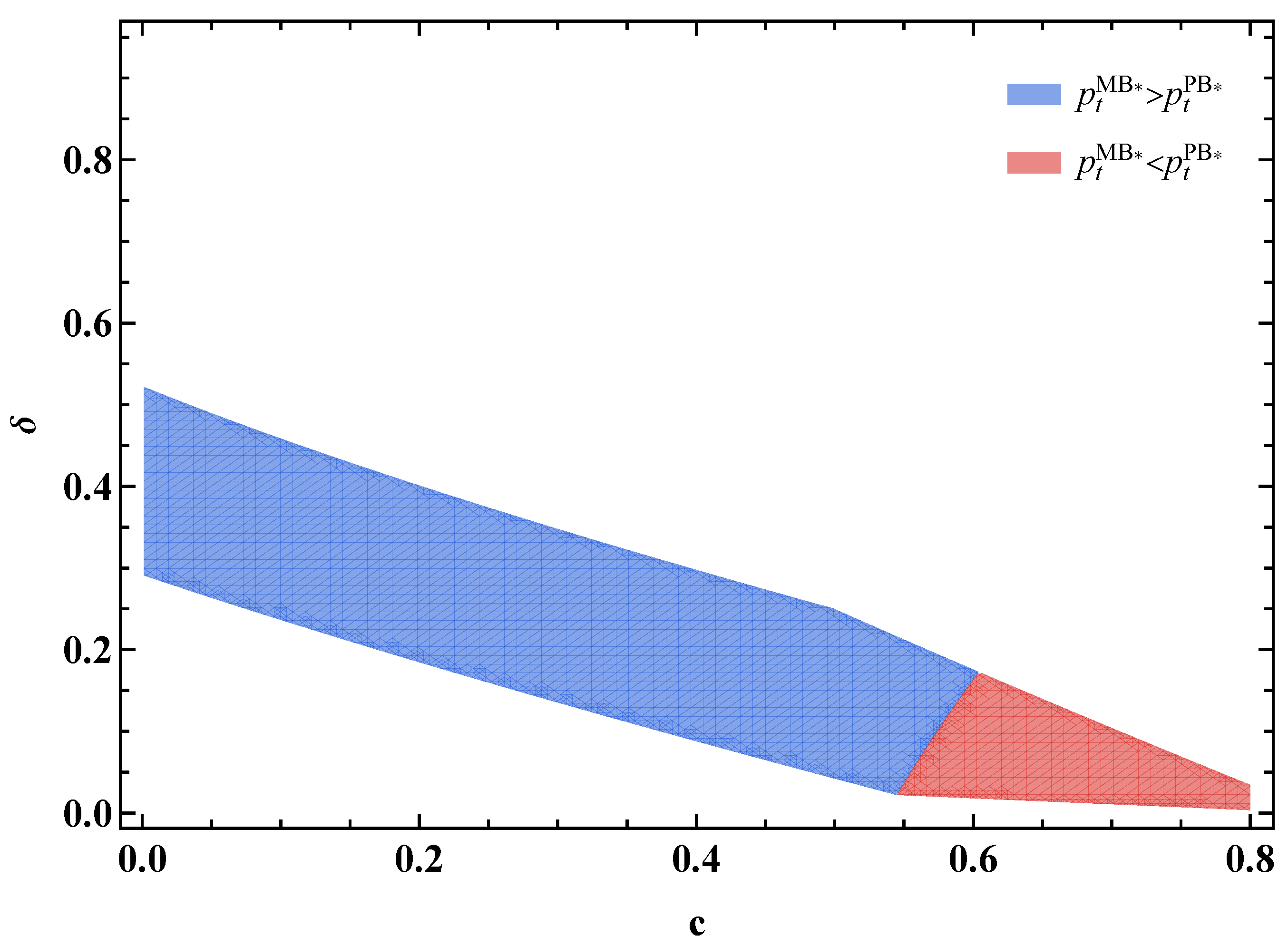
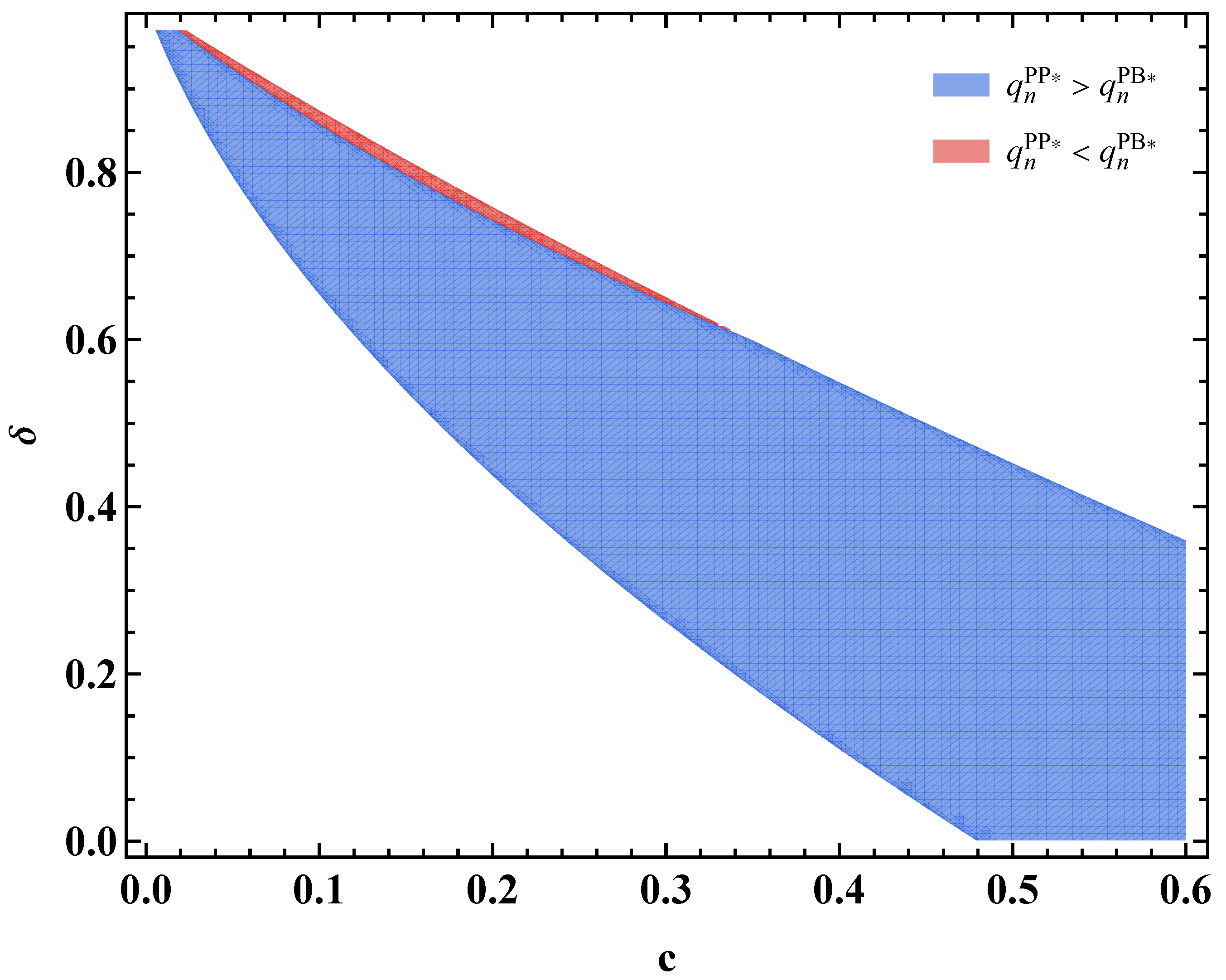
Since it is hard to compare $p_n^{MB\ast }$ and $p_n^{PB\ast }$ analytically, we use a numerical experiment to illustrate their relationship at $\alpha =0.4$ and $\varphi =0.15$, as shown in Figure 2. Contrary to Proposition 2(2), under bank financing, a manufacturer-implemented trade-in no longer always carries the lower new-product price. Once the bank makes the loan, the platform earns only its commission $\varphi p_n$ and not the interest that an expanded demand would generate, so it has little incentive to offer a deep rebate (Figure 3). By contrast, the manufacturer balances the rebate needed to induce replacement against the cost of funding it. A higher residual value raises the required rebate, whereas a lower production cost gives the manufacturer greater room to bear this cost. In the high-residual-value, low-cost region, the manufacturer therefore offers a more generous rebate, which lifts the new-product price through the same mechanism as in Proposition 2(2); over most of the plotted region, the manufacturer-implemented program then carries the higher price. Only in the low-residual-value, high-cost region does the manufacturer’s rebate incentive fade, letting the financing rate take over. Under bank financing, a platform-implemented trade-in carries the higher rate (Proposition 1(2)(ii)). With the rebate playing little role, this higher rate passes through to a higher new-product price. The ordering thus reverts to the platform, $p_n^{PB\ast }$ overtaking $p_n^{MB\ast }$.

5.2.2. Trade-In Rebate

Proposition 3.

(1) Under a fixed trade-in implementer, platform versus bank financing:

• (i) under a manufacturer-implemented trade-in, $p_t^{MP\ast }\ge p_t^{MB\ast }$ if $c\le c_1^I$ and $p_t^{MP\ast }<p_t^{MB\ast }$ otherwise;
• (ii) under a platform-implemented trade-in, $p_t^{PP\ast }\ge p_t^{PB\ast }$ if $c\le c_1^T$ and $p_t^{PP\ast }<p_t^{PB\ast }$ otherwise.
• (2) Under platform financing, $p_t^{MP\ast }<p_t^{PP\ast }$.
• The threshold $c_1^T$ is given in Appendix B.

Proposition 3(1) fixes the trade-in implementer and compares the rebate under platform versus bank financing. The ranking is cost-dependent. The financing cost difference is transmitted through the trade-in implementer’s rebate incentive. The financing source changes the manufacturer’s new-product price and thus the rebate needed to sustain replacement demand, while the implementer weighs this demand gain against the rebate cost. As the production cost changes, this balance shifts, so platform financing induces the larger rebate at low costs, whereas bank financing does so at high costs.

Proposition 3(2) fixes platform financing and compares the rebate under a manufacturer- versus platform-implemented trade-in. The platform-implemented program pays the larger rebate. This is the deeper rebate already at work in Proposition 2(2): when the platform controls the rebate, it uses a larger rebate to expand both its commission and lending returns, whereas the manufacturer must fund the rebate from its own sales margin.

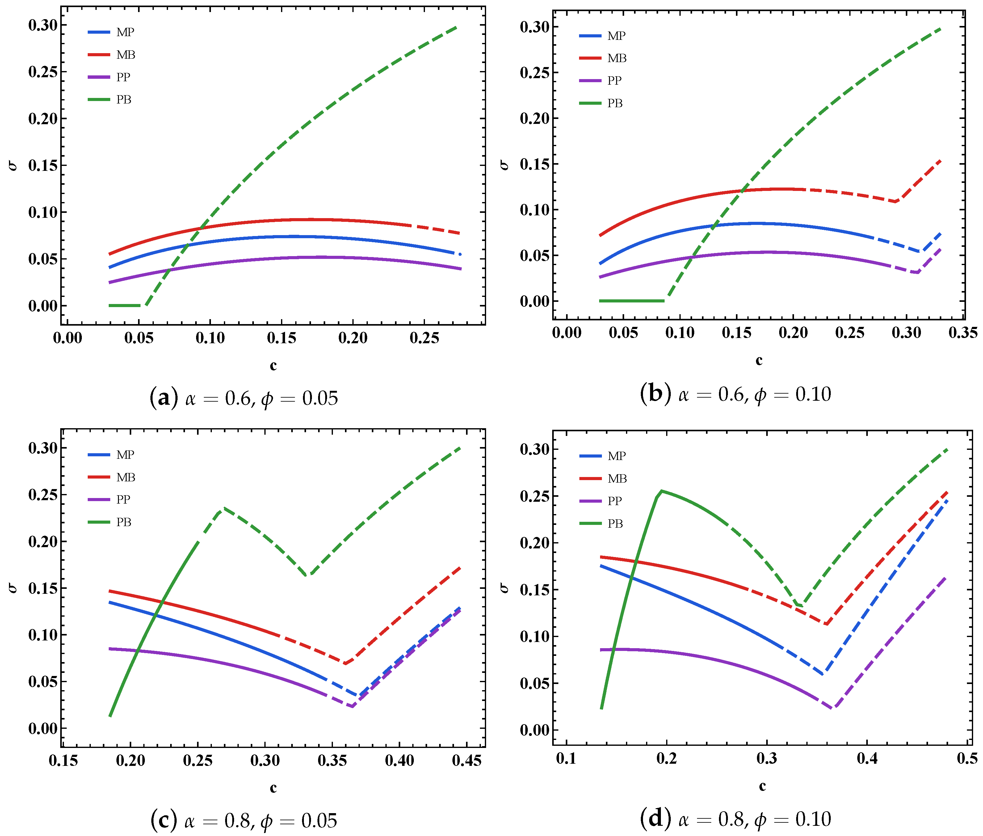
Comparing $p_t^{MB\ast }$ and $p_t^{PB\ast }$ analytically is again hard; Figure 3 plots their ordering at $\alpha =0.4$ and $\varphi =0.15$. As in the price comparison following Figure 2, the manufacturer’s rebate incentive dominates throughout most of the plotted region, making the manufacturer-implemented program more generous; in the low-residual-value, high-production-cost corner, the financing rate effect dominates and the platform-implemented program regains the larger rebate.

5.2.3. Total Demand

Proposition 4.

(1) Under a manufacturer-implemented trade-in, platform versus bank financing: $q_n^{MP\ast }<q_n^{MB\ast }$ if $c<c_1^D$ and $q_n^{MP\ast }\ge q_n^{MB\ast }$ otherwise.

• (2) Under a fixed financing source, manufacturer versus platform trade-in:
• (i) under platform financing, $q_n^{MP\ast }=q_n^{PP\ast }$;
• (ii) under bank financing, $q_n^{MB\ast }\ge q_n^{PB\ast }$ if $c\le c_2^D$ and $q_n^{MB\ast }<q_n^{PB\ast }$ otherwise.
• The thresholds $c_1^D$ and $c_2^D$ are given in Appendix B.

Proposition 4(1) fixes a manufacturer-implemented trade-in and compares total demand under platform versus bank financing. The ranking is cost-dependent, and total demand moves inversely with the financing rate: a higher rate lifts the price and contracts total demand, so the channel with the higher rate yields lower total demand. When the cost is low, the platform’s rate exceeds the bank’s (Proposition 1(1)(i)) and platform financing yields lower total demand; when the cost is high, the platform’s rate is the lower of the two, and platform financing yields higher total demand. This cost-dependent ordering contrasts with Mandal et al. [1], who show that, when two competing third-party sellers both choose the same financing source, their selling quantities are always lower under bank financing than under platform financing.

Proposition 4(2) fixes the financing source and compares the two implementers. Under platform financing, part (2)(i) delivers the notable result: total demand is the same regardless of the implementer. The two programs are far from identical in their prices—a platform-implemented trade-in sets a higher price and pays a larger rebate (Propositions 2 and 3)—yet these differences cancel in the aggregate: the higher new-product price contracts primary demand $q_{nn}$, while the deeper rebate lowers the effective price $p_n-p_t$ and expands replacement demand $q_{nr}$ by exactly the same amount, leaving $q_n$ unchanged. When the platform both lends and earns the commission, the choice of implementer is a pure redistribution of who buys the new product, primary consumers versus replacement consumers, rather than of how many are sold. This cancellation is special to platform financing: the platform’s whole return, interest and commission alike rises with total demand. This exact offset arises when demand is linear and deterministic, the manufacturer finances its entire production through the platform, and the platform leads the game while internalizing both commission and lending returns. By anticipating the manufacturer’s pricing response, the platform adjusts the interest rate and, when it implements the trade-in, the rebate, so that the decrease in primary demand is exactly balanced by the increase in replacement demand. Accordingly, the result applies when demand is stable and predictable and the manufacturer relies entirely on platform financing for production. Under bank financing, the bank earns the interest, whereas the platform earns only the commission, so no single party internalizes both income streams: the platform loses the lending lever that absorbed the implementer’s impact, the gap between the two programs is no longer netted out but passes through to total demand, and part (2)(ii) turns cost-dependent.

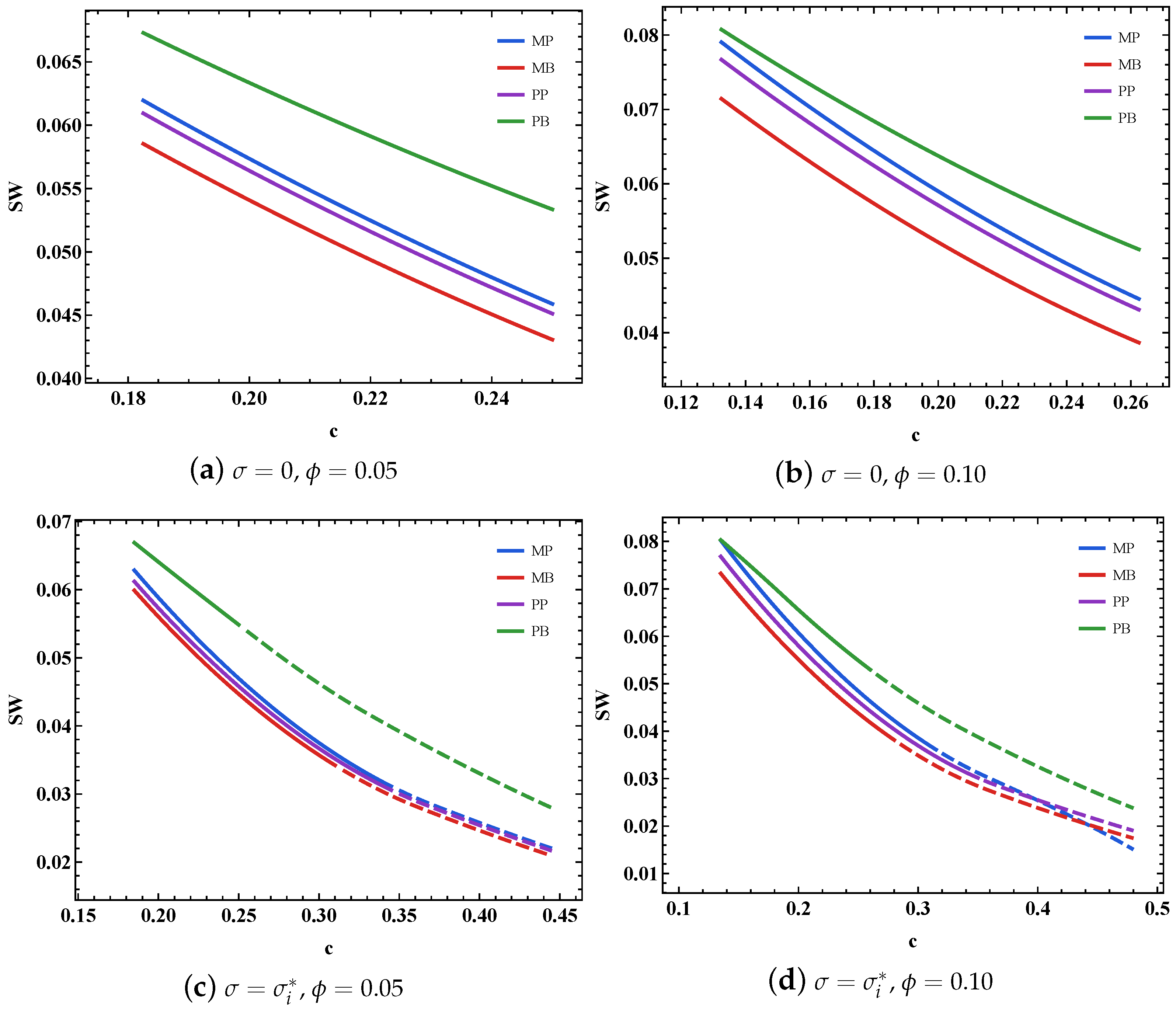
Comparing $q_n^{PP\ast }$ and $q_n^{PB\ast }$ is again analytically intractable; Figure 4 plots their ordering at $\alpha =0.9$ and $\varphi =0.2$. Platform financing yields higher total demand across almost the entire plotted region, driven by the rebate rather than the rate. Under platform financing, the platform sets a generous rebate (Proposition 3(1)(ii)), lowering the effective price and expanding replacement demand; this rebate channel, not the financing rate, keeps platform financing ahead, so total demand here does not follow the rate as it does in part (1). Only in a narrow band along the high-residual-value frontier, where the platform’s rebate advantage narrows, does bank financing yield higher total demand.

5.3. Trade-In Preference

5.3.1. Preferences of the Trade-In Implementers

Proposition 5.

Under platform financing, for the manufacturer, ${\Pi }_m^{MP\ast }>{\Pi }_m^{PP\ast }$; for the platform, ${\Pi }_p^{PP\ast }>{\Pi }_p^{MP\ast }$.

Proposition 5 shows that under platform financing, each member strictly prefers to implement the trade-in itself, unconditionally—independent of the commission rate $\varphi$—so the assignment is a persistent conflict between the two. This unconditional conflict contrasts with the no-financing benchmark presented in Section 6.1 and with Wang et al. [6], who show that under agency selling without financing, the manufacturer’s and platform’s preferences over the trade-in implementer vary with the commission rate. Introducing platform financing into agency selling changes this preference relationship from commission-dependent to parameter-independent. The interest the platform charges on the loan is tied to total demand, a return earned on every unit sold like the retail margin a reseller keeps, so neither member’s preference now hinges on the commission; as under reselling, both always want to run the trade-in themselves. The driver is that the implementer internalizes one extra pricing decision—the rebate—and coordinates it with the lever already in hand: the manufacturer sets $p_n$ and $p_t$ jointly and the platform sets r and $p_t$ jointly. Each is better off as the implementer, so the program becomes a point of conflict rather than a task that either side will delegate.

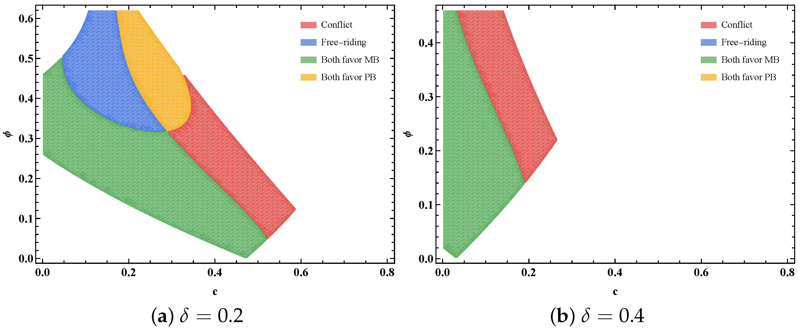
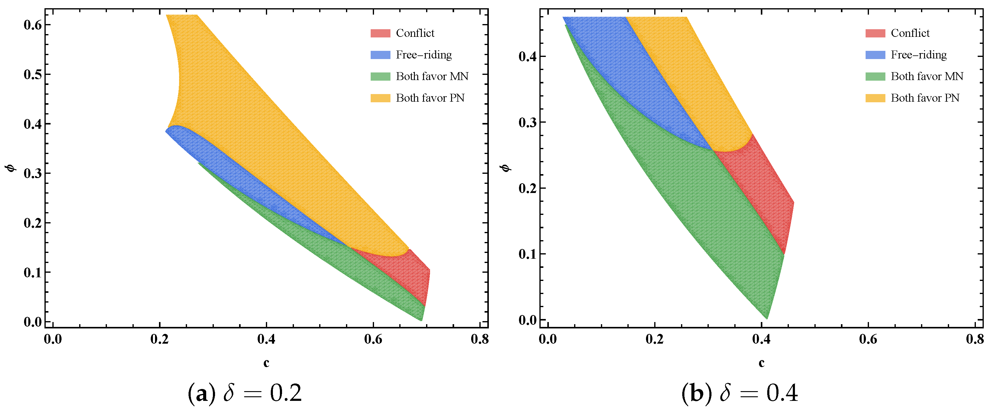
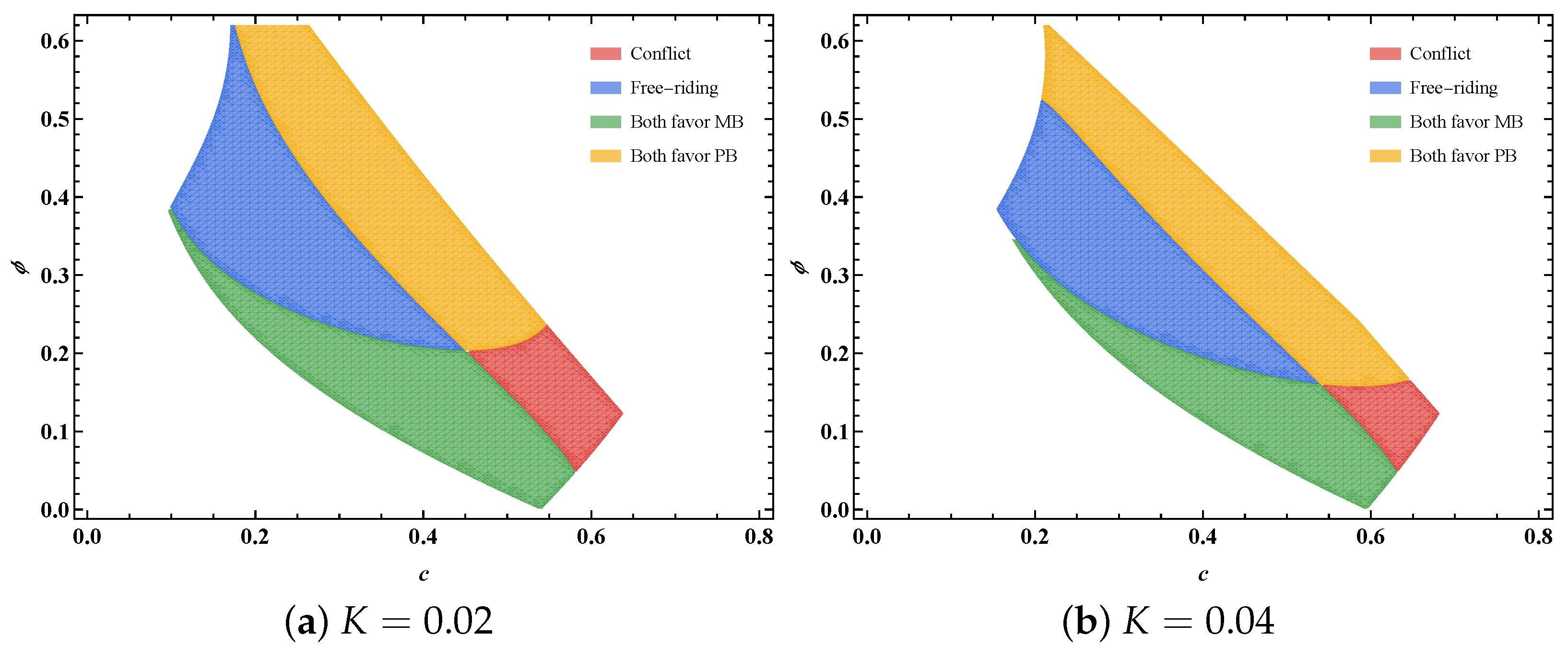
When the bank provides financing, it is difficult to compare the manufacturer’s and platform’s trade-in preferences analytically. We therefore examine their preferences numerically over the feasible region. Figure 5 maps the resulting preference regions over the cost–commission $(c,\varphi )$ plane at $\alpha =0.4$. At a low residual value (panel (a)), all four configurations appear, set by two forces. The first is which implementer generates higher total demand: the manufacturer at low cost and the platform at high cost (Proposition 4(2)(ii)). The second force is the allocation of the rebate cost. This cost weighs more heavily on the party that receives the smaller share of sales revenue: a high commission reduces the manufacturer’s share, $(1-\varphi )p_n$, whereas a low commission reduces the platform’s share, $\varphi p_n$ (as in [6]). At a low cost, total demand is higher under the manufacturer-implemented program, and both members favor it. Raising the commission turns this into mutual free-riding at a low cost, since neither side will fund a rebate that generates little additional demand, with both favoring the platform at an intermediate cost, where total demand under platform implementation is by then higher. Only at a high cost and a modest commission does each prefer to run the program itself, so the platform-financing conflict resurfaces in only one of the four regions. At a high residual value (panel (b)), the trade-in is costly to run and the feasible commissions shrink, collapsing the free-riding and both-favor-platform regions: only the cost-dependent split survives, with the manufacturer-implemented program preferred at low cost and conflict at high cost. These fragmented preferences arise because the bank captures the lending return that platform financing would keep inside the chain. With this profit transferred outside the manufacturer-platform dyad, the preference gaps narrow, and small movements in c and $\varphi$ suffice to reverse them, fragmenting the two members’ choices across the plane rather than aligning them on the commission alone.

5.3.2. The Bank’s Preference over the Trade-In Implementer

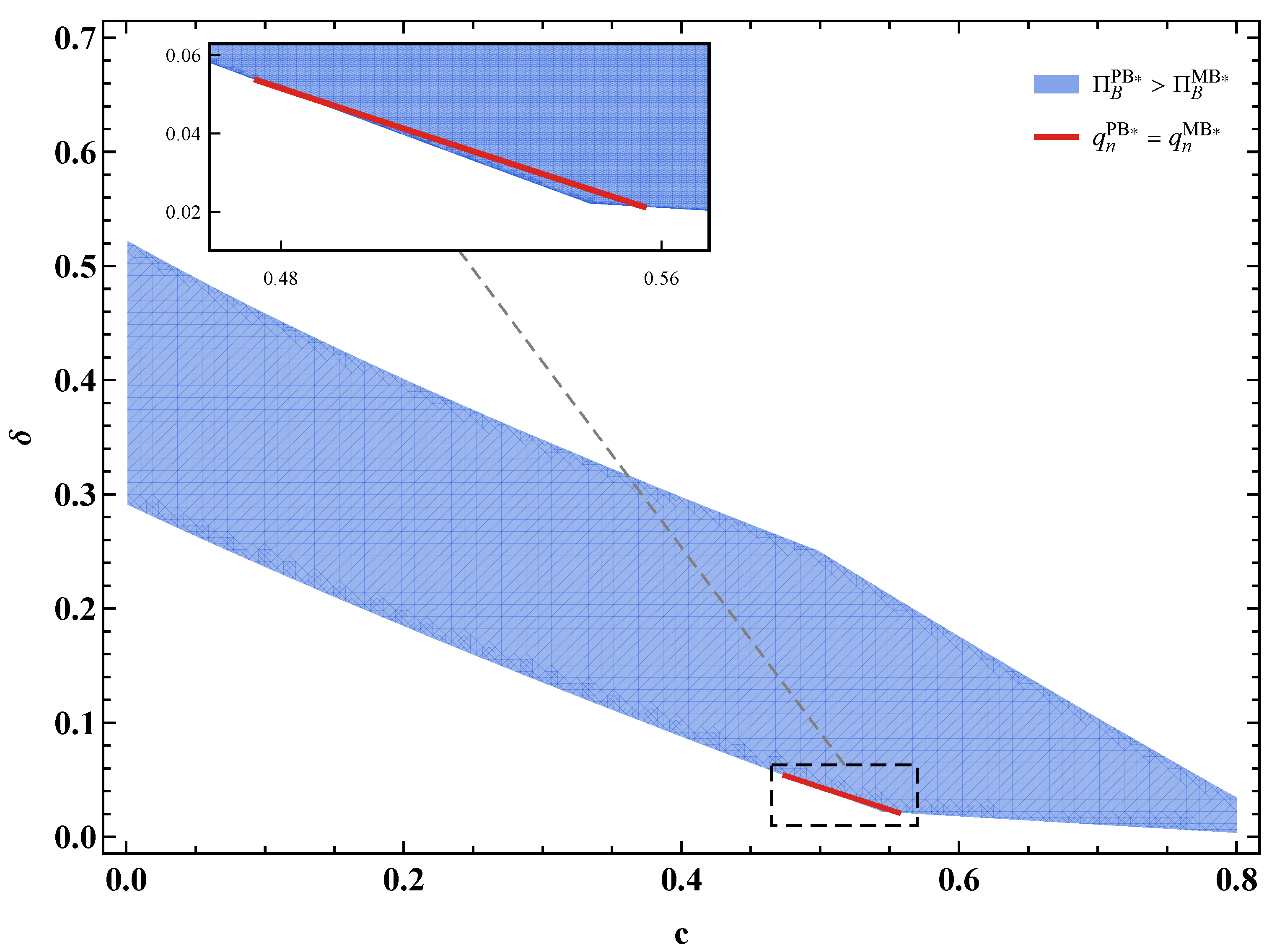
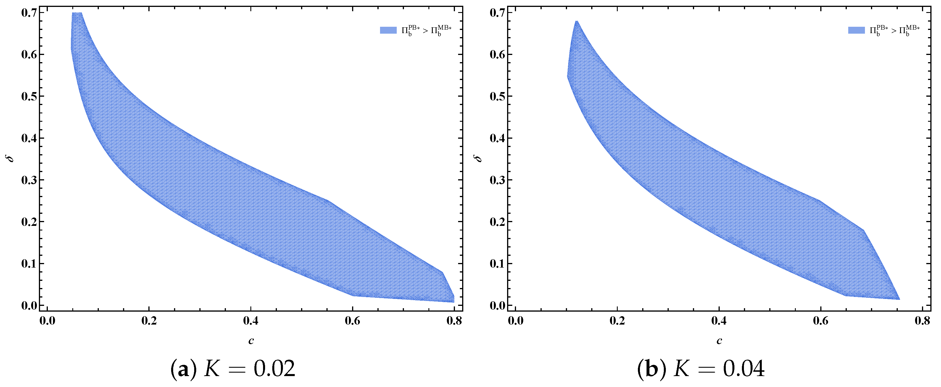
It is hard to rank the bank’s two profits in closed form, so we compare them numerically over the feasible region. Figure 6 reports the comparison in the $(c,\delta )$ plane at $\alpha =0.4$ and $\varphi =0.15$. Over the entire plotted region, the bank strictly prefers the platform to implement the trade-in, ${\Pi }_b^{PB\ast }>{\Pi }_b^{MB\ast }$. This numerical result contrasts with the divided preferences of the manufacturer and the platform in Section 5.3.1.

The bank’s interest rises with both the rate it charges and total demand. The rate favors the platform unambiguously—a platform-implemented trade-in carries the higher rate, $r^{PB\ast }>r^{MB\ast }$ (Proposition 1(2)(ii))—whereas total demand does not, since $q_n^{MB\ast }$ and $q_n^{PB\ast }$ cross at the cost threshold $c_2^D$ (Proposition 4(2)(ii); the red curve in Figure 6, magnified in the inset). Within the plotted region, the rate proves decisive: even below $c_2^D$, where total demand is higher under the manufacturer-implemented program, the higher rate the bank earns under platform implementation more than offsets that small demand advantage.

5.4. Manufacturer’s Financing Channel Choice

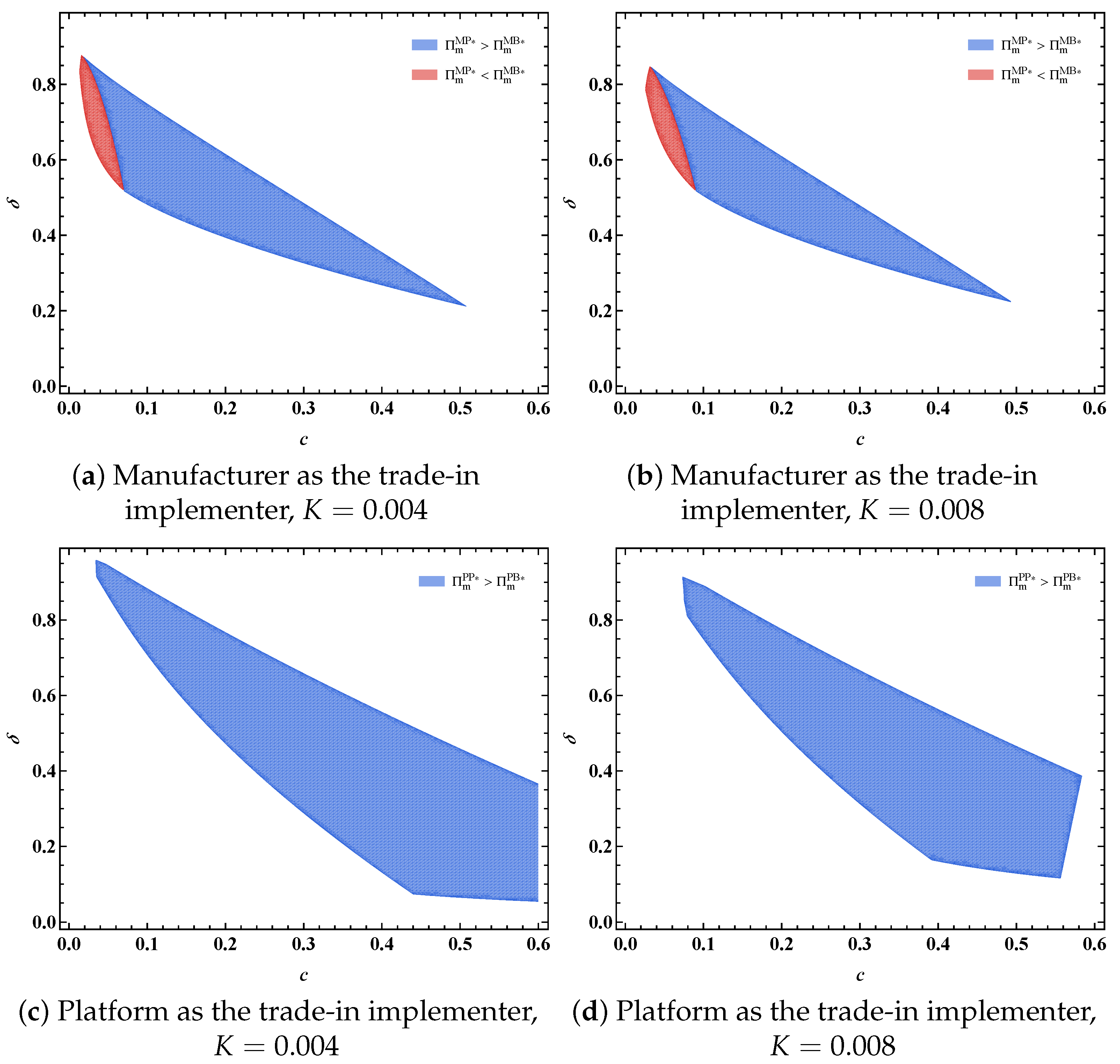
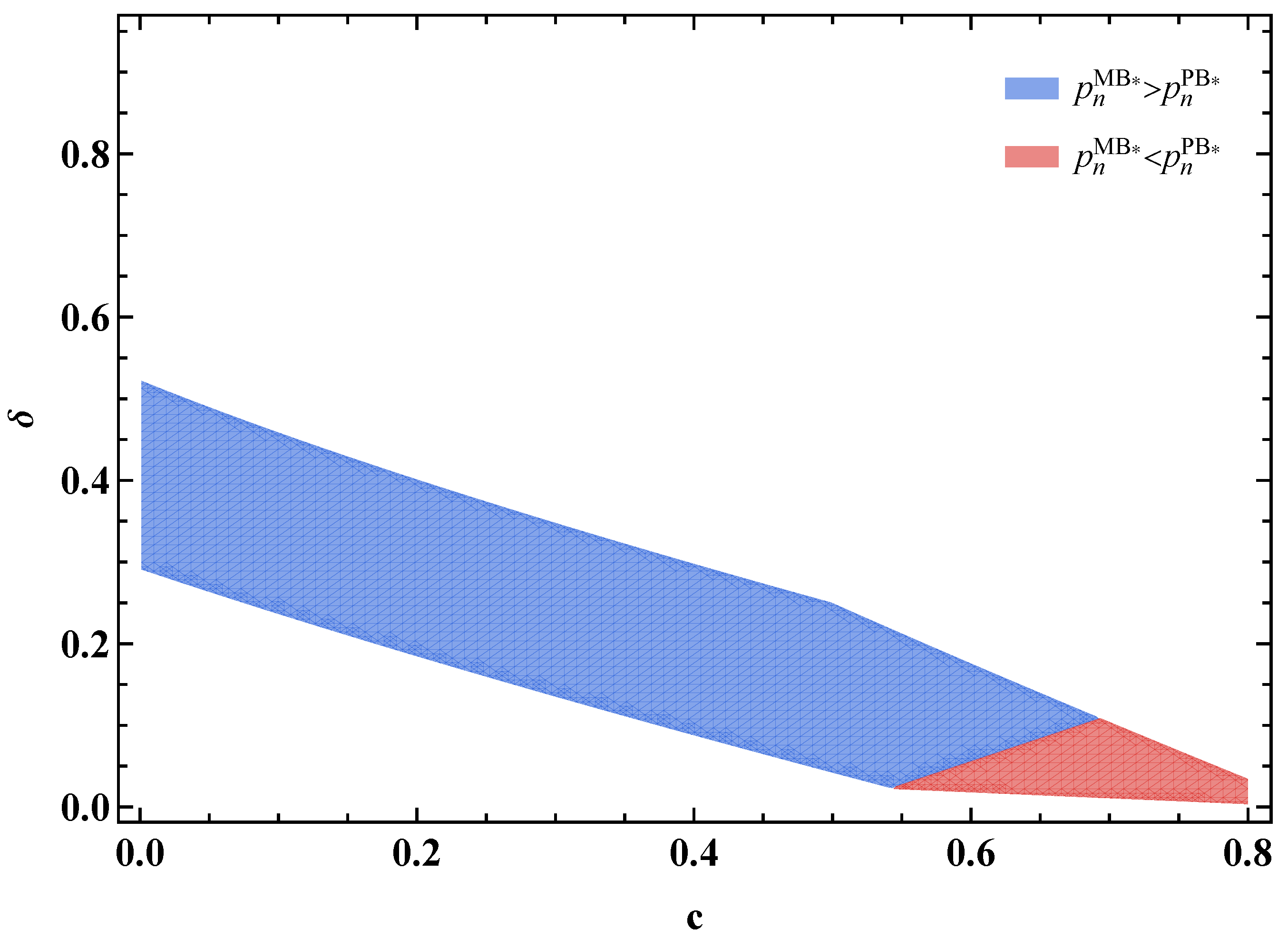
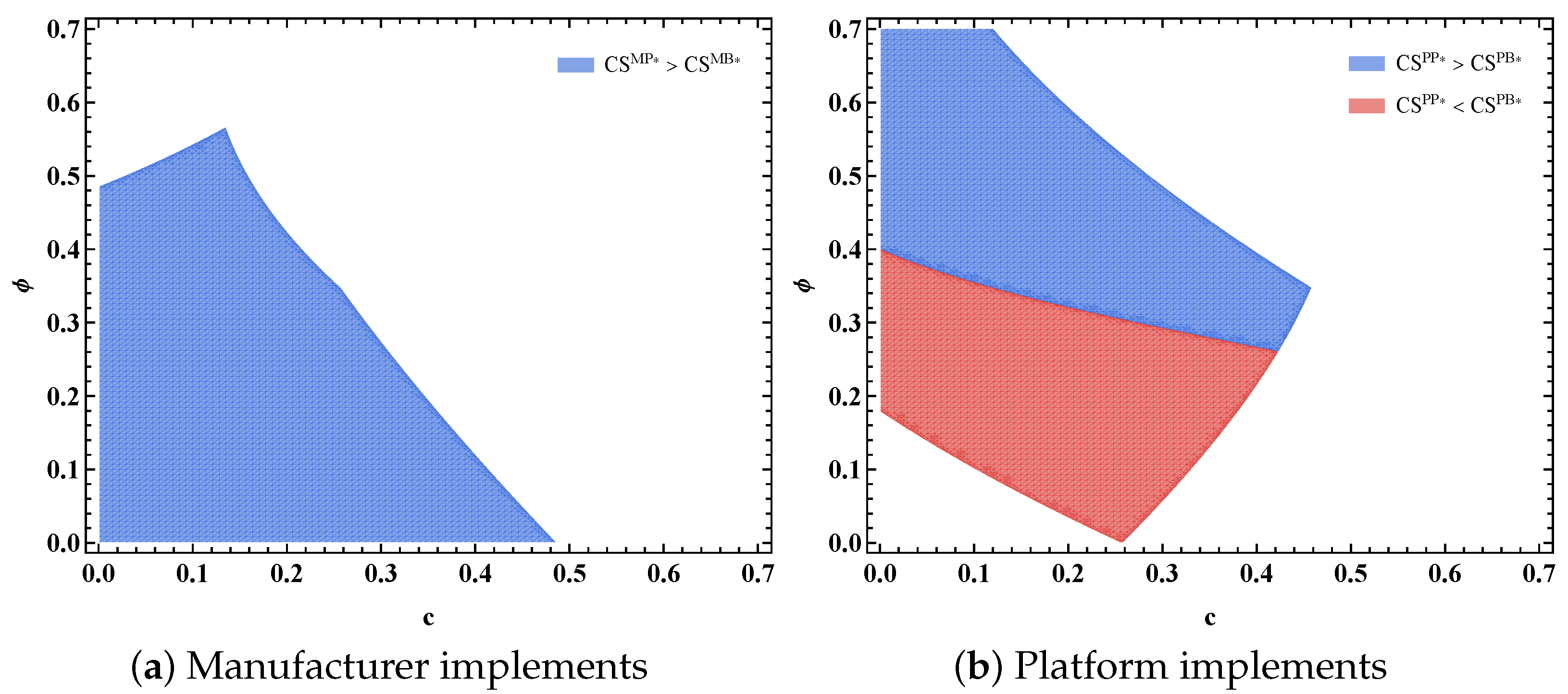
The manufacturer now chooses its financing channel—platform (P) or bank (B)—taking the trade-in implementer as given. It is hard to rank its profit across financing channels in closed form, so we proceed numerically over the feasible region. Figure 7 reports the two comparisons in the $(c,\delta )$ plane at $\alpha =0.9$ and $\varphi =0.2$ (blue: platform financing preferred; red: bank). Under both implementers, platform financing is preferred over most of the region, with the manufacturer turning to the bank only at very low cost when it implements the trade-in itself (panel a) and along the high-residual-value frontier when the platform implements it (panel b). We find that the manufacturer’s financing-channel choice coincides with the total-demand comparison of Section 5.2.3, with panel a matching Proposition 4(1) and panel b matching Figure 4. This numerical result indicates that higher total demand drives the manufacturer’s choice; the forces behind the total-demand comparison in Section 5.2.3 therefore carry over.

5.5. Consumers’ Preference

Following [4], we measure consumers’ preference by the consumer surplus accruing to buyers of the new product: a primary consumer who buys obtains $\theta -p_n$ and a replacement consumer who repurchases obtains $(1-\delta )\theta -(p_n-p_t)$. Consumer surplus is given by the following, evaluated at each scenario’s equilibrium:

$$C{S}^{i\ast }=(1-\alpha )\underset{\mathrm{primary}\mathrm{consumers}}{\underbrace{{\int }_{p_n^{i\ast }}^1\left(\theta -p_n^{i\ast }\right)d\theta }}+\alpha \underset{\mathrm{replacement}\mathrm{consumers}}{\underbrace{{\int }_{{\displaystyle \frac{p_n^{i\ast }-p_t^{i\ast }}{1-\delta }}}^1\left((1-\delta )\theta -p_n^{i\ast }+p_t^{i\ast }\right)d\theta }},i\in \{MP,MB,PP,PB\}.$$

(10)

It is hard to rank consumer surplus across the scenarios in closed form, so we proceed numerically. We examine consumers’ preference along two dimensions—the trade-in implementer and the financing channel—holding one fixed and varying the other, and report the comparisons in the $(c,\varphi )$ plane at $\alpha =0.6$ and $\delta =0.4$.

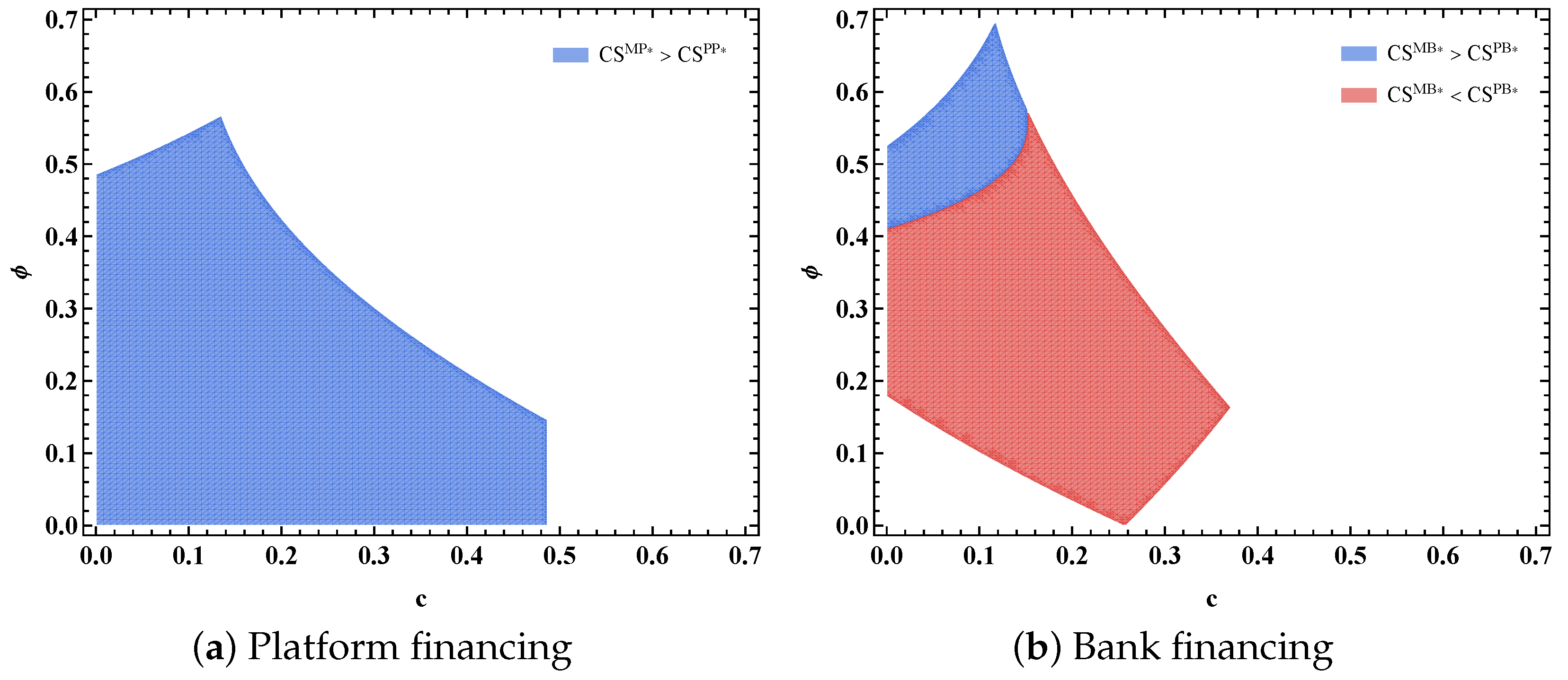
Holding the implementer fixed, we first compare the two financing channels; in Figure 8, blue marks where consumers prefer platform financing and red marks where they prefer bank financing.

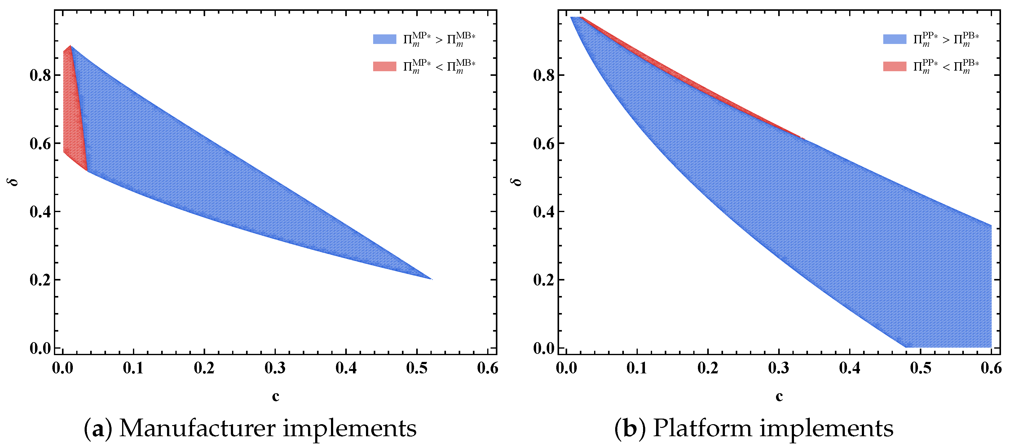
Figure 8 shows consumers preferring platform financing when the manufacturer implements the trade-in (panel a) and shifting their preference with the commission when the platform implements it (panel b). The new-product price is the main driver in both comparisons because it affects both consumer segments, while the rebate may reinforce or offset its effect for replacement consumers. When the manufacturer implements, the platform—earning a commission as well as interest—lends more cheaply here than a bank that maximizes interest alone, so platform financing carries the lower price. Platform financing also carries the lower rebate in this region, which partly offsets its price advantage for replacement consumers; however, the price reduction benefits both consumer segments and therefore dominates. When the platform implements, the comparison turns on the lender’s response to the commission. The bank earns interest alone, so its rate is steadier than the platform’s and, at a low commission, lower; with little commission yet passing into the price, bank financing is then the cheaper channel and consumers are best off under it in the plotted region, $C{S}^{PB\ast }>C{S}^{PP\ast }$. As the commission rises this reverses: under bank financing the manufacturer, squeezed by the commission, lifts its price steeply, while under platform financing the platform cuts its rate sharply to protect the commission it now earns, holding its price down. At a high commission, platform financing is therefore the cheaper channel and, reinforced by its deeper rebate, delivers the larger surplus, $C{S}^{PP\ast }>C{S}^{PB\ast }$.

Holding the financing channel fixed, we then compare the two implementers; in Figure 9, blue marks where consumers prefer the manufacturer-implemented scenario and red marks where they prefer the platform-implemented one.

Figure 9 shows consumers preferring the manufacturer-implemented trade-in under platform financing (panel a) and shifting their preference with the commission under bank financing (panel b). The new-product price remains the main driver because it affects both consumer segments, while the rebate may reinforce or offset this price effect for replacement consumers. Under platform financing, the platform earns on both the loan and the commission, so its return rises with sales, and total demand is the same regardless of the implementer (Proposition 4(2)(i)); a manufacturer- versus platform-implemented trade-in then only trades a lower price (Proposition 2(2)) against a deeper rebate, and because the lower price benefits both consumer segments whereas the deeper rebate benefits only replacement consumers, the price effect dominates and the manufacturer-implemented scenario is the one they favor. Under bank financing, the cheaper scenario changes with the commission. A platform-implemented trade-in leaves the manufacturer setting only the price (the platform fixes the rebate and the bank fixes the rate), so a rising commission passes straight through into a steeply higher price. A manufacturer that also sets the rebate holds two levers and keeps the chain more coordinated, so its price climbs far less. At a low commission, the platform-implemented scenario either carries the lower price or offers a sufficiently deeper rebate to compensate replacement consumers for a small price disadvantage, so consumers prefer it in the plotted region, $C{S}^{PB\ast }>C{S}^{MB\ast }$; at a high commission, its price overtakes the other, and the price loss across both consumer segments dominates the rebate effect, so the ranking reverses, $C{S}^{MB\ast }>C{S}^{PB\ast }$.

6. Extensions

We consider three extensions to the baseline model: a no-financing benchmark, a government trade-in subsidy, and the manufacturer’s initial capital. They respectively isolate the role of financing, introduce a policy instrument, and examine whether the baseline findings remain robust when the manufacturer can finance part of its production internally.

6.1. No-Financing Benchmark

To isolate the role of financing, we consider a benchmark in which the manufacturer has sufficient internal capital to cover its production costs. Removing the financing stage reduces the four baseline scenarios to two: the manufacturer implements the trade-in program and jointly determines $p_n$ and $p_t$ (scenario $MN$), or the platform implements the program and determines $p_t$ before the manufacturer sets $p_n$ (scenario $PN$). Although the equilibrium decisions can be derived analytically, the two members’ joint preference regions do not admit transparent closed-form partitions. We therefore use numerical experiments to characterize these regions. To facilitate a direct comparison with the bank financing case in Figure 5, we use the same calibration: $\alpha =0.4$, with $\delta =0.2$ and $\delta =0.4$ in the two panels, and plot the joint preferences over the $(c,\varphi )$ plane.

Figure 10 shows that without financing, the manufacturer’s and platform’s joint preference configuration is parameter-dependent. All four configurations arise within the plotted common feasible region under both parameter settings. By contrast, Proposition 5 shows that only the conflict configuration arises under platform financing. Comparing Figure 10 and Figure 5, when the residual value is low, the four preference regions under bank financing closely resemble those without financing. When the residual value is high, however, bank financing changes this pattern: the free-riding and both-favor-$PB$ configurations disappear over the plotted common feasible region. This change occurs because a higher residual value increases the rebate cost borne by the implementer. Under this condition, part of the surplus that the manufacturer and platform would retain under no financing is instead allocated to the bank as a lending return, thereby substantially altering both members’ preferences over the trade-in implementer.

6.2. Government Trade-In Subsidy

We extend the baseline model to incorporate a government trade-in subsidy, a policy lever that is widely used in China to stimulate consumer-goods demand. We examine how the subsidy interacts with the four supply-chain structures. The government pays a replacement consumer who trades in a used product with and purchases the new product a subsidy proportional to the new-product price, $\sigma p_n$, at a rate $\sigma \in [0,1)$; primary consumers, who own no used product, are ineligible. The subsidy lowers a replacement consumer’s effective price to $(1-\sigma )p_n-p_t$, so the replacement demand becomes $q_{nr}=\alpha \left(1-{\displaystyle \frac{(1-\sigma )p_n-p_t}{1-\delta }}\right)$, while the primary demand $q_{nn}=(1-\alpha )(1-p_n)$ is unchanged. Each member’s objective retains the form of Section 4, and we re-solve the equilibrium of every scenario under the subsidy.

Social welfare in scenario i sums consumer surplus and the profits of the manufacturer, the platform, and the bank and subtracts the government’s subsidy outlay:

$$S{W}^{i\ast }=C{S}^{i\ast }+{\Pi }_m^{i\ast }+{\Pi }_p^{i\ast }+{\Pi }_b^{i\ast }-\sigma p_n^{i\ast }{q}_{nr}^{i\ast },i\in \left\{MP,MB,PP,PB\right\},$$

(11)

where ${\Pi }_b^{i\ast }=0$ under platform financing; the last term is the government’s subsidy payment; and consumer surplus, now including the subsidy received by each replacement consumer, is

$$C{S}^{i\ast }=(1-\alpha ){\int }_{p_n^{i\ast }}^1\left(\theta -p_n^{i\ast }\right)d\theta +\alpha {\int }_{{\displaystyle \frac{(1-\sigma )p_n^{i\ast }-p_t^{i\ast }}{1-\delta }}}^1\left((1-\delta )\theta -(1-\sigma )p_n^{i\ast }+p_t^{i\ast }\right)d\theta .$$

(12)

6.2.1. Optimal Trade-In Subsidy

Deriving tractable analytical solutions to the welfare optimization problem is difficult. Thus, we use numerical experiments to examine the subsidy rate. Let ${\sigma }_i^{\ast }$ denote the subsidy rate associated with the maximum or supremum of social welfare $S{W}^{i\ast }\left(\sigma \right)$ in scenario i, taken over the range of $\sigma$ on which the scenario remains feasible. When the welfare supremum occurs at an open feasibility boundary, the subsidy rate and the corresponding welfare reported in Figure 11 and Figure 12 represent the limiting values approached from within the feasible region. Because subsidy rates in practice are moderate (around 15%) (https://www.ndrc.gov.cn/xxgk/jd/jd/202512/t20251230_1402853.html (accessed on 5 August 2026)), we restrict the rate to $\sigma \le 0.3$. Figure 11 reports ${\sigma }_i^{\ast }$ as the production cost c varies for $\alpha \in \{0.6,0.8\}$ and $\varphi \in \{0.05,0.10\}$ at $\delta =0.6$. In each panel, a solid segment marks the production costs at which the scenario is feasible without the subsidy, so setting $\sigma =0$ remains an available choice. A dashed segment marks the costs at which the scenario is sustained only by the subsidy. The subsidy can therefore expand the production-cost range over which the trade-in program remains feasible.

Figure 11 shows that the welfare-maximizing subsidy rates of scenarios $MP$, $MB$, and $PP$ vary with the production cost in a similar pattern; scenario $PB$ departs from it. The departure reflects how decision rights are allocated. $PB$ is the only scenario in which three self-interested members each control one lever: the bank sets the financing rate, the platform sets the rebate, and the manufacturer sets the new-product price. In every other scenario, two of the levers are concentrated in one member. This allocation changes how the equilibrium responds to the subsidy.

For scenario $PB$, under the parameter settings shown in Figure 11, when the replacement fraction $\alpha$ and the production cost are both small, the government’s optimal choice is not to subsidize (${\sigma }_{PB}^{\ast }=0$). The reason is twofold. First, at a low production cost, the subsidy provides only a weak stimulus. Second, the dispersed decisions weaken this stimulus further. The subsidy therefore does not raise social welfare over the plotted low-cost range. As the production cost increases, the optimal rate rises steeply. The reason is that the subsidy serves mainly to preserve replacement demand, which would otherwise vanish. Replacement demand is fragile because the platform earns no interest income under scenario $PB$. When $\alpha$ is small, the limited potential commission gain from replacement demand gives the platform little incentive to provide rebate support. A higher cost raises the new-product price, so the subsidy required to sustain this demand increases with the cost.

However, under the $\alpha =0.8$ calibration, the zero-subsidy optimum disappears, because the surplus gain of replacement consumers becomes more pronounced; the optimal rate instead varies with the cost in a more complex way. The rate first rises steeply. With a large replacement segment, the platform is inclined to capture part of the subsidy by cutting its rebate, and the feasible subsidy range is bounded by the requirement $p_t>0$. As the production cost increases further, the associated increase in the new-product price induces the platform to offer a larger rebate to sustain replacement purchases. The rebate is therefore positive at the interior welfare optimum, so the constraint $p_t>0$ no longer binds. The government then lowers the subsidy rate to maximize social welfare. At still higher costs, the optimal rate turns upward again: the trade-in program, with its high cost and low return, is neglected by the platform, and the government must raise the subsidy once more to sustain it.

For the remaining three scenarios, under the calibrations in Figure 11, when $\alpha$ and the production cost are both small, the optimal rate increases with the cost. In this range, prices are low, and a cost increase erodes replacement demand more sharply than primary demand, so the government raises the rate to pull this demand back. As the cost grows further, the new-product price rises substantially; the subsidy-induced loss of primary-consumer surplus becomes more pronounced relative to the replacement-consumer gain, and the welfare-maximizing rate turns downward. When the cost is very high, the subsidy again serves mainly to sustain the trade-in program, and the rate rises with the cost, a stage most visible when $\alpha$ is large. Under the $\alpha =0.8$ calibration, the low-cost increasing segment is absent or only weakly visible over the common feasible cost range for the following reasons. First, this range excludes much of the lower-cost increase. Second, when the replacement segment is large, a further increase in the subsidy rate generates a much larger fiscal outlay than the accompanying gain in replacement-consumer surplus over the plotted declining regions. As the production cost rises, the subsidy also becomes less effective in supporting firms’ profits, so the government does not raise the rate further.

Figure 11 also ranks the subsidy levels across the four scenarios: over most of the cost range in which all four curves overlap, the optimal rate is highest under $PB$, followed by $MB$ and then $MP$, being lowest under $PP$. As discussed above, the trade-in program receives the least internal support under $PB$, so the largest subsidy is required to bring its potential into play. The rate under $MB$ exceeds that under $MP$ because, consistent with Proposition 1, over the cost range shown, the bank, which earns no commission, charges a higher interest rate than the lending platform; the heavier financing cost feeds into the new-product price, and a larger subsidy is needed to offset it. $PP$, where the platform holds both the rate and the rebate and earns both income streams, calls for the smallest subsidy over most of the plotted overlap range: the additional welfare that the subsidy can deliver is limited. At the low end of the cost range, in contrast, the rate under $PB$ is the lowest of the four. The cause is the same: the platform neglects the returns associated with the trade-in program, so the subsidy delivers little welfare gain, and a higher subsidy rate would violate the requirement $p_t>0$.

6.2.2. How Does the Subsidy Affect Social Welfare?

We then examine how the subsidy affects social welfare and which structure a welfare-oriented government should favor. To observe welfare over a larger cost range, we consider only $\alpha =0.8$; a larger $\alpha$ is also consistent with today’s increasingly saturated durable-goods markets. Figure 12a,b report the benchmark welfare without the subsidy over the cost range on which all four scenarios are feasible at $\sigma =0$; Figure 12c,d report each structure’s maximum or supremum welfare, denoted by $S{W}^{i\ast }\left({\sigma }_i^{\ast }\right)$, with solid and dashed segments carrying the same meaning as in Figure 11.

Figure 12 shows the same ranking under the plotted parameter settings: over most of the cost range in which all four curves overlap, scenario $PB$ delivers the highest social welfare, followed by $MP$ and $PP$, and $MB$ delivers the lowest. Under these calibrations, the ranking is therefore rooted in the structures themselves rather than in the subsidy: the optimized subsidy weakly increases each structure’s welfare where $\sigma =0$ is feasible and greatly extends the cost range over which the four structures coexist, but preserves this ordering over most of the plotted overlap range. $PB$ is thus the structure that a welfare-oriented government should favor over most of the plotted overlap range under these calibrations. Welfare tracks how well the two consumer segments are served. Scenario $PB$ attains the highest welfare because its supply chain centers on the primary market: primary consumers own no used product, and their valuations are not discounted by the residual value, so each sale to them generates a larger consumer surplus. The ranking of the remaining scenarios follows from the same tradeoff between primary and replacement demand. The subsidy promotes replacement purchases and suppresses primary demand, but these shifts are small relative to the structural differences.

These results carry two implications for the government under the plotted parameter settings. The subsidy rate should be tailored to the supply-chain structure rather than set uniformly: the welfare-maximizing rate is the highest under $PB$ and the lowest under $PP$ over most of the cost range in which all four curves overlap, so a single flat rate cannot fit all structures. Moreover, the displayed low-cost results for $PB$ show that subsidizing is not always beneficial: when the platform implements the trade-in under bank financing and the production cost is low, the replacement-consumer gain does not offset the loss of primary-consumer surplus and the optimal rate is zero, so the government should assess whether the induced demand reallocation raises welfare before offering it.

6.3. Manufacturer’s Positive Initial Capital

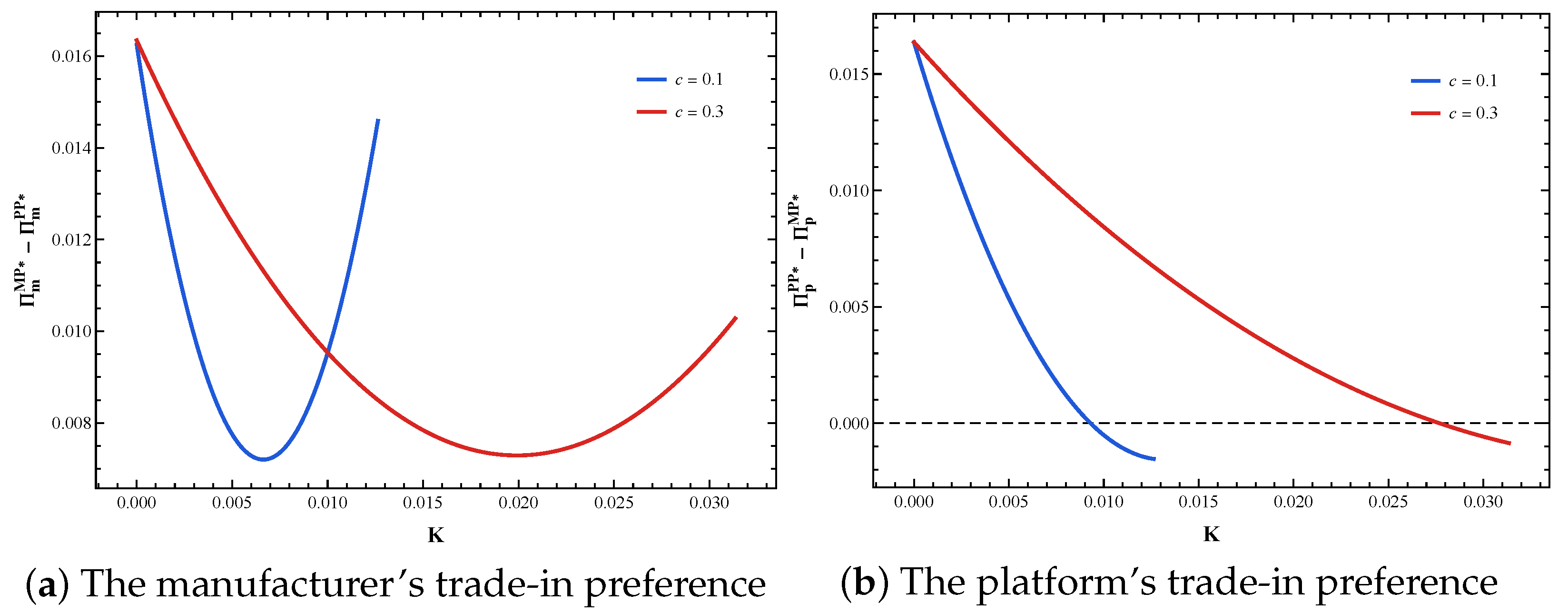
In the baseline model, the capital-constrained manufacturer has no initial capital and therefore finances its entire production expenditure, $c{q}_n$. We relax this assumption by endowing the manufacturer with initial capital K, where $0<K<c{q}_n$. The lender finances only the shortfall $c{q}_n-K$, and interest is charged on this amount. All other model assumptions and the sequence of decisions remain unchanged. Introducing initial capital makes the equilibrium profit comparisons considerably more involved and does not yield economically transparent closed-form preference conditions. We therefore use numerical experiments over the common feasible region to examine whether the core findings of this study continue to hold.

First, we examine the manufacturer’s and platform’s preferences over the trade-in implementer under platform financing. We set $\alpha =0.8$, $\varphi =0.05$, and $\delta =0.6$ and consider $c\in \{0.1,0.3\}$. Figure 13 shows that for both cost levels, introducing initial capital does not change the manufacturer’s preference over the respective plotted common feasible regions: the manufacturer continues to prefer implementing the trade-in program itself. The platform, however, comes to prefer the manufacturer to implement the program once the manufacturer’s initial capital is sufficiently high. As K increases, the manufacturer relies less on platform financing and retains more of the sales gains generated by its trade-in decision. The platform can then earn commission revenue from these additional sales without bearing the rebate cost. Under bank financing, we follow panel (a) of Figure 5 and set $\alpha =0.4$ and $\delta =0.2$. The joint preference configuration remains consistent with the $K=0$ benchmark: all four configurations continue to arise over the plotted common feasible region at both $K=0.02$ and $K=0.04$ in Figure 14.

Second, we examine whether the bank’s preference over the trade-in implementer changes with the manufacturer’s initial capital. Following Figure 6, we set $\alpha =0.4$ and $\varphi =0.15$. Figure 15 shows that the bank continues to prefer the platform as the trade-in implementer over the plotted common feasible region at both $K=0.02$ and $K=0.04$, consistent with the main result in Section 5.3.2.

Third, we examine the manufacturer’s financing-channel preference while holding the trade-in implementer fixed. Following Figure 7, we set $\alpha =0.9$ and $\varphi =0.2$, compare platform and bank financing over the $(c,\delta )$ plane, and consider $K\in \{0.004,0.008\}$. These smaller values of K retain a nonempty common feasible region for the $PP$–$PB$ comparison. Figure 16 shows that when the manufacturer implements the trade-in, its financing-channel preference remains consistent with the baseline pattern: regions favoring platform and bank financing continue to arise. When the platform implements the trade-in program, however, the small bank-financing region in Figure 7b disappears, and the manufacturer prefers platform financing throughout the plotted common feasible region. The reason is as follows. Compared with the bank, which earns only interest income, the platform also earns commission revenue and internalizes the sales response to its rebate. As K increases and the loan principal $c{q}_n-K$ decreases, a high financing rate generates less lending return because it applies to a smaller principal while continuing to suppress sales and commission revenue. The platform therefore relies more on commission income and the demand expansion generated by the trade-in program and reduces its financing rate more strongly than the bank. This adjustment lowers the manufacturer’s financing burden and makes platform financing more profitable for the manufacturer under the parameter settings considered.

7. Conclusions

This study examined the interplay of financing (by the platform or a bank) and trade-in implementation (by the manufacturer or the platform) in an agency supply chain with a capital-constrained manufacturer, and the interaction of the two dimensions yielded four scenarios. Under these four scenarios, we developed a game-theoretic framework with replacement and primary consumers, in which the platform and/or the bank act as leaders and the manufacturer acts as the follower. We then derived the equilibrium interest rate and pricing decisions in each scenario and combined analytical comparisons with numerical experiments to investigate how the two dimensions interact in shaping prices, demand, and the parties’ trade-in and financing preferences.

Our analysis yields several findings. First, the robustness of the equilibrium comparisons differs across the two dimensions: switching the financing channel generally reverses the ranking of the decisions as the production cost varies, whereas switching the trade-in implementer leaves several comparisons unchanged or pinned down by the equilibrium structure, particularly under platform financing. Second, under platform financing, a platform-implemented program embeds a cross-subsidy: it raises the new-product price and enlarges the rebate; counterintuitively, the two effects offset, and total new-product demand is independent of the implementer; once a bank finances production, this neutrality disappears. Third, financing reshapes the contest over implementation. Under platform financing, both the manufacturer and the platform want to run the program themselves, a preference that does not hinge on the commission rate, so the trade-in becomes an object of contention rather than delegation; under bank financing, where the lending return accrues to an outside bank, this parameter-independent conflict disappears and the willingness to run the program varies with the production cost and the residual value of used products. Fourth, under the reported parameter settings, the remaining preferences follow identifiable levers. The manufacturer’s channel choice tracks total demand over the feasible region, and the bank prefers a platform-implemented program, which sustains the higher lending rate. Consumers’ preferences are fixed in two of the four comparisons, namely, platform financing when the manufacturer implements the trade-in and manufacturer implementation when the platform finances production; in the other two comparisons, it shifts with the commission: when the platform implements, consumers prefer bank financing at a low commission and platform financing at a high one, and under bank financing, they prefer platform implementation at a low commission and manufacturer implementation at a high one. Finally, the reported numerical experiments indicate that the welfare-maximizing subsidy rate varies with both the supply chain structure and the production cost, peaking under $PB$, bottoming under $PP$, and vanishing under $PB$ at low costs; over most of the plotted overlap range, welfare follows the same ranking with or without the subsidy, with $PB$ highest and $MB$ lowest, while the subsidy generally raises its level and widens the workable cost range.

These results offer guidance for firms and policymakers. (1) A capital-constrained manufacturer should make its financing and trade-in decisions jointly: different trade-in implementers and different lenders lead it to different choices. (2) A platform that both lends and charges a commission should manage the interest rate, the commission, and, when it implements the program, the rebate as one system: optimizing one lever while ignoring the others can overturn the intended outcome. (3) The trade-in subsidy calls for differentiated design rather than a uniform rate: the welfare-maximizing rate depends on who implements the program and who finances production, and it moves with the production cost. In particular, when the replacement segment and the production cost are both small, withholding the subsidy may be the better choice, since the gain to replacement consumers does not offset the loss of primary-consumer surplus; for high-cost products, keeping the subsidy in place is essential, since without it, the trade-in program cannot operate.

This study can be extended in several directions. First, we assume deterministic demand; incorporating demand uncertainty would let the financing and trade-in decisions hedge against random replacement volumes and clarify how risk shifts the financing-channel and implementation choices. Second, we treat the quality difference between the new and used products as exogenous; endogenizing product-quality improvement would link the trade-in rebate to the manufacturer’s innovation decision and consumers’ replacement incentives. Third, our model features a single manufacturer; extending it to competing manufacturers on the same platform would show how competition reshapes the financing channel choice and the trade-in implementation.