Subsample Analysis of Oil Revenue Shocks and Macroeconomic Policy Transmission

Abstract

This research examines the impact of positive crude oil revenue shocks on Russia’s macroeconomic policy and economic development, analyzes the effects of macroeconomic policy on the economy, and compares these effects across two subsamples (2005–2013 and 2015–2019). The study proves that the full 2005–2019 model fails to capture the transmission responses of policy and macroeconomic variables after the significant structural shift in the post-2014 period, while subsample models each provide a better fit and more accurate results. Our empirical research provides the following insights: First, after 2014, fiscal expansion shifted from an anti-inflationary tool to an inflationary driver as well as a depreciating force on the national currency. Second, after 2014 the monetary policy’s tight stance became explicitly anti-inflationary compared with its direct opposite effects before 2014. Third, after 2014, the central bank’s more dominant inflation-targeting regime tightened the constraints on fiscal policy. Fourth, the Russian Federation’s economic dependence on oil diminished after 2014. Finally, macroeconomic policy (government expenditure and key interest rate) shifted from procyclical to countercyclical in response to oil revenue shocks after 2014.

1. Introduction

The core aim of macroeconomic policy remains long-term stability and growth. However, in most resource-dependent nations, this pursuit is overwhelmingly dominated by the challenge of managing volatile hydrocarbon revenues. Macroeconomic policy often reacts to oil price shocks, leading to procyclical, distortionary outcomes that can undermine broader economic resilience. Therefore, assessing policy failures and their consequences for the domestic economy requires examining macroeconomic policy together with oil price or revenue dynamics.

This study examines the Russian Federation as a resource-dependent economy whose macroeconomic performance is strongly shaped by fluctuations in commodity prices and energy revenues. Indeed, the Russian Federation, with significant oil reserves, demonstrates a high budget dependence: 35–50% of federal budget revenues are traditionally derived from crude oil exports [1].

The relevant literature on the topic can be broadly classified into two streams (the overview of selected empirical studies can be found in Appendix A.5). The first strand of literature examines the oil-macroeconomy nexus. It confirms Russia’s oil dependency but reveals distinct and ambiguous implications. For example, Nyangarika and Tang [2] and Alekhina and Yoshio [1] highlighted the Russian economy’s dependence on crude oil price shocks. Drygalla also provided evidence on the direct impact of oil prices on the exchange rate, output, and inflation rates [3]. Ito highlighted the impact of crude oil prices on manufacturing output in Russia [4]. Balashova and Seretis found that positive oil price shocks led to increases in key economic indicators [5]. Benedictow studied the impact of crude oil revenue on Russian macroeconomic indicators and noted that the Russian economy is highly dependent on crude oil revenue; however, significant economic development occurred beyond the crude oil revenue booms [6]. On the other hand, Idrisov stated that the impact of crude oil prices on Russian economic development dramatically decreased after 2000 [7]. Lomonosov found that positive oil-price shocks matter for the Russian economy during global economic booms [8]. Wang found a causal relationship between crude oil prices and unemployment in Russia, with crude oil price shocks increasing unemployment, particularly in 2009, 2016, and 2020 [9]. Su found that busts in crude oil prices amplify wage arrears in Russia [10]. Yang stated that crude oil prices’ negative and positive shocks are more of a blessing for Russian output since both positively affect Russian GDP [11].

The second branch of the literature studies oil-driven fiscal and monetary policies. Several studies have concluded that fiscal policy is often procyclical in resource-exporting countries [12,13,14,15,16]. Within the Russian context, few studies have analyzed fiscal and monetary policy responses to crude oil price fluctuations, such as those by Benedictow, who found that government expenditure in Russia increases in response to higher oil revenues, but not proportionally, suggesting a countercyclical accumulation of oil revenues in the national fund [6]. Sohag also found countercyclical features of fiscal borrowing to manage the government budget deficit [17]. On the other hand, Gurvich [18] argues that Russian fiscal policy is procyclical, which is associated with dependence on oil revenues. Moreover, Tuzova and Qayum [19] and Ito [4] found that government expenditure and consumption respond procyclically to positive oil-price shocks in the short term. Finally, Çiçekçi and Gaygısız noted the procyclicality of Russian fiscal policy in response to crude oil price shocks, even in the presence of a welfare fund [20].

Regarding monetary policy, Tyunova argues that Russia’s key interest rate became countercyclical after the shift to inflation targeting in 2014 [21]. However, Jin and Xiong [22] and Yildirim and Guloglu [23] found procyclicality of Russia’s key interest rate. Some scholars implicitly show that the key rate reacts to positive shocks in a procyclical manner in the short term in Russia [1,3].

However, the uniqueness of the Russian case lies in the combination of global economic shocks and internal structural transformations, most pronounced after 2014. This period is characterized not only by geopolitical changes and the imposition of international sanctions, capital outflows, and Russian national currency depreciation but also by fundamental shifts in macroeconomic policy (see Figure 1).

In November 2014, Elvira Nabiullina, the head of the Russian Central Bank, in a policy outlook called “Main directions of the unified state monetary policy of the central bank of the Russian Federation 2015–2016–2017,” announced the completion of monetary policy’s transition to inflation targeting and spoke of geopolitical challenges, the exhaustion of the traditional growth channels, and the consequent need for deep structural economic transformation [24]. Furthermore, following the dramatic drop in oil revenues in 2014–2016 and the resulting budget deficit, fiscal policy later shifted toward consolidation of government spending. However, existing studies of Russian macroeconomics generally do not distinguish between pre- and post-2014 dynamics, lacking knowledge of how the relationships between oil shocks and macroeconomic policy have changed. Our study addresses this gap by systematically comparing these two periods.

We hypothesize that the events of 2014 marked a qualitative structural rupture in the Russian economy and that the subsequent structural transformation of macroeconomic policy significantly altered the channels and efficiency of oil revenue transmission into macroeconomic and broader economic indicators. The primary objective of this study is not to identify a structural break per se, but rather to conduct a comparative analysis of two periods—before and after 2014—to identify qualitative changes in oil revenue and macroeconomic policy impact on the economic development.

The study is similar to Tyunova but introduces three key modifications to refine the analysis of Russia’s oil macroeconomy and oil-driven macroeconomic policy nexus. First, we employ a crude oil revenue endogenous variable rather than the oil price, which is exogenous to the Russian economy [1]. Second, we incorporate government expenditure to account for the fiscal policy response to oil revenue shocks and the independent macroeconomic effects of fiscal impulses. Third, following Tyunova’s own methodological suggestion that testing the impact of monetary policy inflation targeting requires more stable observations, we exclude the turbulent structural break period of 2014.

The analysis employs a structural Bayesian Hierarchical Vector Autoregression (BVAR) model. This framework adopts a flexible, data-driven approach, allowing each model specification to automatically learn the optimal degree of shrinkage for the identified subsamples. This method prevents overfitting and overparameterization—ensuring that the data, rather than a dominant prior, inform the posterior—thereby allowing for a more robust qualitative comparative analysis. Consequently, the study compares three baseline specifications:

• The combined model (2005–2019)—serves as a basis for comparison
• The pre-2014 model (2005–2013)—reflects the period with reactive fiscal and monetary policies and Russian fast economic development.
• The post-2014 model (2015–2019)—takes into account the inflation targeting regime and the transition to fiscal policy consolidation with structural shifts in the Russian macroeconomy.

The empirical results confirm a significant difference between the pre- and post-2014 samples. The study shows that the combined model (2005–2019) cannot capture the nuances of divergent crude oil, fiscal, and monetary structural shocks to macroeconomic indicators.

Following the IRF and FEVD analysis, we documented empirical evidence that:

• Before 2014, macroeconomic policy (government expenditure and key interest rate) demonstrated predominantly procyclical responses to shocks in oil revenues. Since 2014, there has been an increase in countercyclicality in the response of macroeconomic policy to oil revenue booms.

The paper also presents a detailed analysis of the transmission channels of the impact of shocks from oil revenues and macroeconomic policy on the Russian macroeconomy, confirming the following empirical patterns:

• Russia’s economic dependence on oil diminished after 2014, as evidenced by the exchange rate of domestic currency and the unemployment rate.

In addition, Russian macroeconomic policy provides divergent shocks across two periods. The study documented empirical evidence that:

• After 2014, fiscal expansion has shifted from an anti-inflationary tool into an inflationary driver and a catalyst for currency depreciation.

The study offers empirical evidence on the key interest rate:

• After 2014, the monetary policy stance became explicitly anti-inflationary.

Moreover, the research found the evidence on Russian macroeconomic interconnections.

• Post-2014, fiscal policy became increasingly constrained by the Central Bank’s more dominant inflation targeting regime.

The remainder of this paper is structured as follows: Section 2 contains on dataset and the BVAR model; Section 3 presents a comparative analysis of IRFs and FEVDs. Section 4 discusses the main findings, and Section 5 concludes the study.

2. Materials and Methods

2.1. Baseline Model

Consider a structural vector autoregression (VAR) model:

$$y_t= \mathrm{c}+A_1{y}_{t-1}+A_2{y}_{t-2}\dots A_p{y}_{t-p}+{\epsilon }_t,$$

(1)

where $y_t$ is a $k\times 1$ variables set, $\mathrm{c}$ is an $k\times 1$ intercept vector, $A_1\dots A_p$ is a $k\times k$ coefficient matrix, and ${\epsilon }_t$ is a $k\times 1$ vector of exogenous Gaussian shocks with zero mean and variance-covariance matrix $Ʃ$. We impose an additional structure on the models to guide the parameters toward a more parsimonious benchmark, minimize estimation errors, and improve structural inference. Therefore, we employ a Bayesian hierarchical approach to avoid unreasonable hyperparameter choices unsupported by the data [25] as cited in ref. [26]. This framework employs a flexible, data-driven approach, where each model specification automatically learns the optimal shrinkage degree for its subsample. Therefore, the hyperparameters are treated as additional system parameters:

$$p\left(\gamma |y\right)\propto p\left(y|\theta ,\gamma \right)p\left(\theta |\gamma \right)p\left(\gamma \right),$$

(2)

where $y={(y_{p+1},\dots , y_{\mathrm{\top }})}^{\mathrm{\top }}$ denoted $\theta$ which are $A_1\dots A_p$ and $Ʃ$ of the VAR model in Equation (1) and $\gamma$ are hyperparameters.

The left-hand side of the posterior distribution of the hyperparameters $\gamma$ in Equation (2) is marginalized with respect to the parameters $\theta$ in the marginal likelihood (ML) equation:

$$p(y|\gamma ) = \int p\left(y|\theta ,\gamma \right)p\left(\theta |\gamma \right)d\theta ,$$

(3)

$p\left(y\right|\gamma )$ is marginal with respect to the parameters $\theta$, but conditional on the hyperparameters $\gamma$. ML allows estimating the likelihood of the data for each possible $\gamma$; thus, the model hyperparameters are automatically estimated, accounting for their uncertainty. In the model, a Markov Chain Monte Carlo (MCMC) algorithm is used. Specifically, the model uses the Metropolis–Hastings (MH) algorithm to sample $\gamma$, and Gibbs steps to sample $\theta$ conditionally on the current draw of hyperparameters. Thus, the joint posterior distribution is constructed as follows:

$$p\left(\theta ,\gamma |y\right)\propto p\left(y|\theta ,\gamma \right)p\left(\theta |\gamma \right)p\left(\gamma \right),$$

(4)

After MCMC sampling is completed, the $\theta$ components are retained from the full samples and used to compute IRFs and FEVDs.

2.2. Model Variables Justification

This study uses Cholesky factorization to identify structural shocks of the variables. First, in the literature, most scholars consider international oil prices to provide a vector autoregression analysis [1,2,3,7,19,23]. However, crude oil revenues have an advantage over crude oil prices because they are endogenous to the Russian economy, including fluctuations in oil prices and changes in oil production. Furthermore, even during periods of high oil prices, revenue can still fall short due to sanctions-related constraints. These factors significantly influence fiscal variables and economic activities.

In this study, the variable oil revenue refers to federal budget revenues collected by the Russian tax system from oil production and exports. The term “oil” was originally stated in the Russian federal budget (The Russian federal budget structure was amended several times during 2005–2019, and the final version of 2019 consists of 27 revenue categories with 2179 subpoints. The term “oil” was unchanged during 2005–2019.), refers to the revenue category named “Taxes, fees and regular payments for the use of natural resources (Although a 2017 amendment to the budget code (art. 96.6) consolidated all revenues from oil, natural gas, and petroleum products into a single “oil and gas revenues” category, the Russian Ministry of Finance continues to publish disaggregated data.)”.

To ensure comparability between the two sub-period models, a common lag order was adopted for both specifications. While the Bayesian information criterion (BIC) was restricted to a maximum of five lags to avoid overparameterization, it suggested optimal lag orders of two for the pre-2014 period and one for the post-2014 period. While some studies analyzing the Russian economy with monthly VAR models use 1 or 2 lags [1,23], we follow the principle emphasized by Kilian and Lütkepohl, who argue that a higher lag order is preferable for better capturing the dynamics of macroeconomic variables [27]. However, our subsamples are relatively small (99 observations in the pre-2014 period and 60 in the post-2014 period), which imposes a practical constraint. Using too many lags would overparameterize the models—especially the post-2014 subsample—raising concerns about the curse of dimensionality even with Bayesian methods. Conversely, using too few lags, as stated with BIC risks, leaves residual autocorrelation and misses important delayed effects. We therefore aim to select the maximum feasible lag length given our data limitations. Consequently, a lag order of three is selected. This specification captures effects over a quarterly horizon while avoiding overfitting in our limited samples. The final specification with three lags produces statistically satisfactory results, as evidenced by the absence of significant residual autocorrelation, confirming that the chosen lag structure adequately captures the underlying data-generating process.

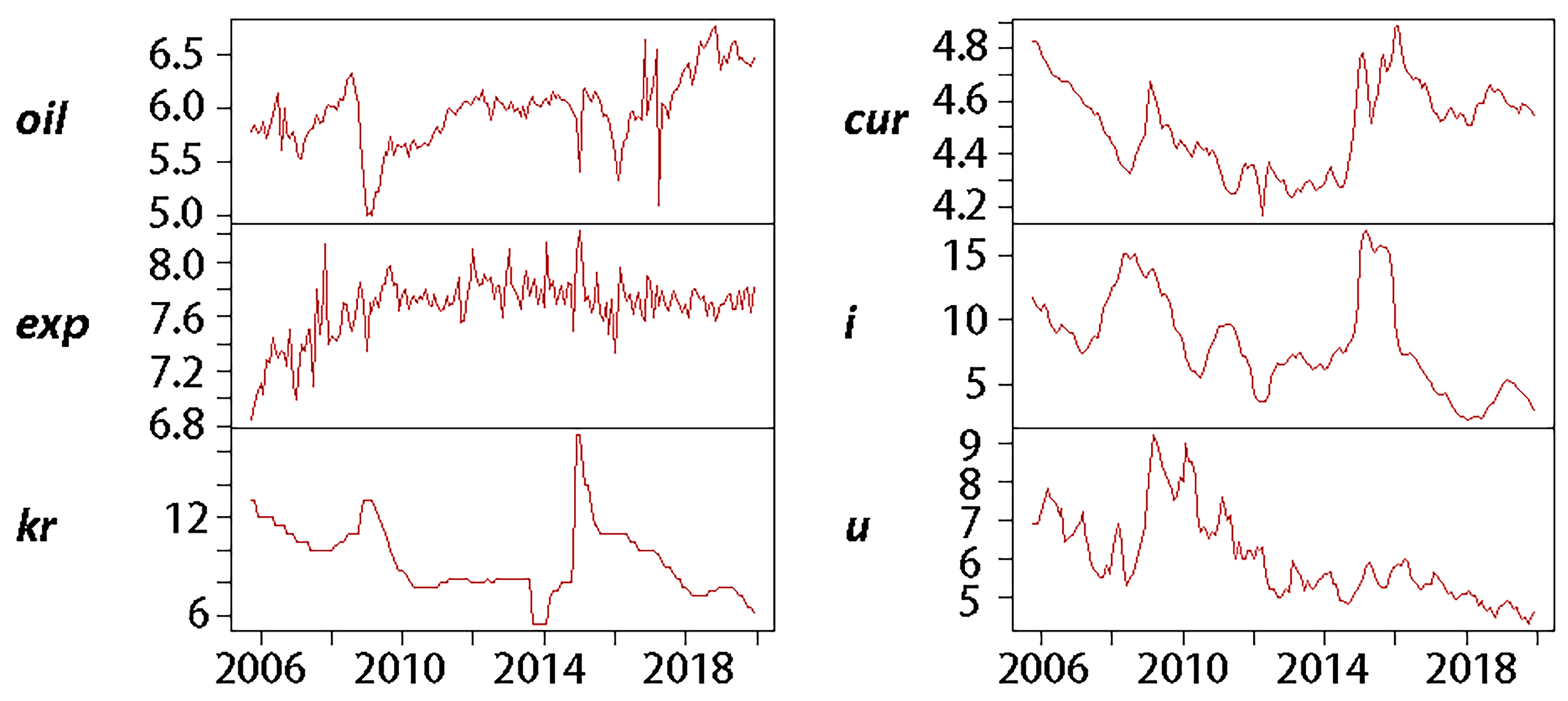
Data for ${(oil}_t)$ and ${(exp}_t)$ were collected from the Ministry of Finance’s monthly reports on the execution of the Russian federal budget. Government expenditures were deseasonalized using a moving average to eliminate an institutional feature that hindered the analysis, as expenditure data exploded toward the end of the year due to budget execution and utilization (the time series are visualized in Figure A1 and Figure A2). Data on ${(kr}_t)$ and ${(cur}_t)$ were collected from the official website of the Central Bank of the Russian Federation. The year-on-year inflation rate ($i_t$) was calculated from the monthly Consumer Price Index (CPI) published on the official website of the Federal State Statistics Service. The data for ($u_t$) was also collected from the Federal State Statistics Service. All variables were adjusted to the CPI index for December 2024 and transformed using natural logarithms, except for ${kr}_t$, $i_t$, and $u_t$, which are expressed in levels (see variables description in

Table 1. Real variable description.

Variable	Description	Transformation
${\mathrm{o}\mathrm{i}\mathrm{l}}_{\mathrm{t}}$	Crude oil revenues in billions of rubles	Log
${\mathrm{e}\mathrm{x}\mathrm{p}}_{\mathrm{t}}$	Public expenditure in billions of rubles	Log
${\mathrm{k}\mathrm{r}}_{\mathrm{t}}$	Central policy key rate	levels
${\mathrm{c}\mathrm{u}\mathrm{r}}_{\mathrm{t}}$	National currency exchange rate against the USD	Log
${\mathrm{i}}_{\mathrm{t}}$	Year-to-year inflation rate	Levels
${\mathrm{u}}_{\mathrm{t}}$	Unemployment rate	Levels

and descriptive statistics in

Table A1. Descriptive statistics of the dataset 2005–2019.

	Mean	Median	SD	Variance	Min	Max	Skewness	Kurtosis
Oil revenue	5.973	6.002	0.335	0.113	4.995	6.763	−0.243	0.564
Total expenditure	7.672	7.701	0.226	0.051	6.846	8.227	−1.070	1.869
Key rate	9.377	8.750	2.096	4.391	5.500	17.000	0.753	0.849
Exchange rate	4.504	4.526	0.166	0.028	4.165	4.883	0.086	−0.987
Inflation	8.134	7.384	3.764	14.165	2.197	16.926	0.523	−0.558
Unemployment	5.978	5.620	1.101	1.212	4.290	9.200	0.892	0.057

,

Table A2. Descriptive statistics of the dataset 2005–2013.

	Mean	Median	SD	Variance	Min	Max	Skewness	Kurtosis
Oil revenue	5.840	5.889	0.263	0.069	4.995	6.331	−1.086	1.439
Total expenditure	7.626	7.688	0.264	0.070	6.836	8.117	−0.863	0.426
Key rate	9.525	9.000	1.856	3.446	5.500	13.000	0.120	−0.754
Exchange rate	4.444	4.420	0.161	0.026	4.165	4.826	0.629	−0.596
Inflation	9.023	8.797	2.958	8.750	3.574	15.144	0.366	−0.660
Unemployment	6.578	6.500	1.054	1.111	5.000	9.200	0.493	−0.588

and

Table A3. Descriptive statistics of the dataset 2014–2019.

	Mean	Median	SD	Variance	Min	Max	Skewness	Kurtosis
Oil revenue	6.175	6.179	0.369	0.136	5.092	6.763	−0.691	0.108
Total expenditure	7.721	7.719	0.118	0.014	7.379	8.270	1.427	6.677
Key rate	9.358	9.000	2.235	4.994	6.250	17.000	1.035	1.077
Exchange rate	4.628	4.593	0.092	0.008	4.510	4.883	0.907	0.105
Inflation	6.734	4.829	4.751	22.575	2.197	16.926	1.121	−0.287
Unemployment	5.148	5.170	0.440	0.194	4.290	5.990	0.075	−0.977

). This treatment and no other transformation of the variable during Bayesian VAR analysis is consistent with Sims [28].

Unit root tests (ADF and KPSS) established that all variables are non-stationary in levels but become stationary after first differencing. Given the I(1) properties of the data, the Johansen cointegration procedure was employed, which revealed the presence of at least one long-run cointegrating relationship among the variables. Such properties of variables became a basis for further prior selection. (The results for unit root and cointegration tests are provided in Appendix A.3).

2.3. Identification of Structural Shocks

2.3.1. Cholesky Factorization

Within the Cholesky identification scheme, we assume a specific contemporaneous ordering grounded in institutional and economic logic. Government expenditure is ordered second because it is often formulated within the constraints of fiscal space shaped by federal revenues. The key policy interest rate is assumed to adjust to the inflationary consequences of fiscal operations.

Finally, we provide no structural interpretation of the macroeconomic variables and adopt the following conventional order: exchange rate, inflation rate, and unemployment rate.

$$y_t=\left[\begin{array}{c}\begin{array}{c}\begin{array}{c}{oil}_t\\ {exp}_t\\ {kr}_t\end{array}\\ {cur}_t\\ i_t\end{array}\\ u_t\end{array}\right],$$

(5)

The robustness of the results is evaluated by re-estimating the models with different variable orderings. The tested orderings are: (1) placing inflation and exchange rate variables ahead of the key interest rate, (2) swapping the sequence of the ruble exchange rate and inflation, and (3) swapping the sequence of key interest rate and government expenditure. The results show that these changes in the identification scheme do not materially affect the impulse response patterns of the Russian economy to macroeconomic policy and oil revenue shocks. The only exceptions are the responses of ($i_t$) in the pre-2014 period and to (${cur}_t$) in the post-2014 period following (${kr}_t$) shocks. For these specific cases, the response paths and overall tendencies remain the same but exhibit a slightly diminished magnitude. (The variables order sensitivity-checks were provided in Appendix D).

2.3.2. Sign and Zero Restriction

In the Russian economic context, the contemporaneous relationships between fiscal variables, monetary policy, and the exchange rate are complex and often subject to debate, as policy reactions can be rapid and interest rates may co-move with the exchange rate within the same period. To address this identification challenge, we additionally employ a sign and zero restriction strategy. This approach partially combines the logic of a Cholesky ordering but imposes no restrictions on the interactions between crude oil revenues, policy variables, and the exchange rate and imposes our intuitions on directional impact of shocks of variables in the system. To ensure full identification of the BVAR, we follow the standard requirement of imposing at least $k \ast (k-1)/2$ restrictions, with a maximum of $k-j$ zero restrictions in the j-th column. Therefore, the sign and zero restrictions on the elements of the restriction matrix are summarized in Equation (5):

$$\left(\begin{array}{c}\begin{array}{c}\begin{array}{c}{u}_t\\ i_t\\ {cur}_t\end{array}\\ {kr}_t\\ {exp}_t\end{array}\\ {oil}_t\end{array}\right)= \begin{array}{c}\begin{array}{cccccc}{\epsilon }_t^u& {\epsilon }_t^i& {\epsilon }_t^{cur}& {\epsilon }_t^{kr}& {\epsilon }_t^{exp}& {\epsilon }_t^{oil}\end{array}\\ \left[\begin{array}{cccccc}+& b_{12}^0& b_{13}^0& +& b_{15}^0& b_{16}^0\\ -& +& +& b_{24}^0& b_{25}^0& b_{26}^0\\ 0& +& +& b_{34}^0& b_{35}^0& b_{36}^0\\ 0& +& b_{43}^0& +& b_{45}^0& b_{46}^0\\ 0& 0& b_{53}^0& b_{54}^0& +& b_{56}^0\\ 0& 0& +& 0& 0& +\end{array}\right]\end{array}$$

(6)

We further assume that all variables respond positively to their own structural shocks; thus, the diagonal elements of the impact matrix ($b_{11}^0$, $b_{22}^0$, $b_{33}^0$, $b_{44}^0$, $b_{55}^0$, and $b_{66}^0$) are restricted to be positive. With regard to oil revenues, we posit that shocks from all other variables affect them only with lags, except for the exchange rate. A positive exchange rate shock—a depreciation of the ruble—can raise oil revenues within the same month. This reflects the institutional feature of Russia’s mineral extraction tax, which is calculated based on the Urals crude price and the exchange rate prevailing at the end of the tax period. Therefore, $b_{63}^0$ is restricted to be positive and $b_{61}^0$, $b_{62}^0$, $b_{64}^0$, ${\mathrm{and} b}_{65}^0$ are restricted to zero. Conversely, shocks from crude oil to all other variables remain unrestricted; hence, coefficients of the matrix $b_{16}^0$, $b_{26}^0$, $b_{36}^0$, $b_{46}^0$, and $b_{56}^0$ remain unrestricted.

The responses of all macroeconomic variables ($b_{15}^0$, $b_{25}^0$, $b_{35}^0$, and $b_{45}^0$) to a shock in public expenditure are left unrestricted. Responses of macroeconomic variables to shocks in key interest rates are also unrestricted ($b_{15}^0$, $b_{25}^0$, ${\mathrm{and} b}_{35}^0)$, except that we impose a positive effect on the unemployment rate ($b_{14}^0$), consistent with the view that a monetary tightening raises unemployment.

We allow positive exchange rate shocks (depreciation) to raise inflation contemporaneously ($b_{14}^0$). Inflation, in turn, is restricted from affecting public expenditure ($b_{52}^0$) within the same period but is permitted to raise the key interest rate ($b_{32}^0$) and depreciate the exchange rate ($b_{22}^0)$.

Finally, the unemployment rate is restricted from contemporaneously affecting public expenditure ($b_{51}^0$), the key interest rate ($b_{41}^0$), and the exchange rate ($b_{31}^0$). However, it is allowed to negatively affect inflation ($b_{21}^0$).

2.4. Prior Specification

The study considers the Minnesota prior as a baseline for vector autoregression specification. This choice is critical, as it enables stable estimation and mitigates overfitting despite the relatively limited number of observations available. The Minnesota prior, proposed by Litterman, assumes that individual variables follow random walk processes [29]. This specification is known for its effectiveness in forecasting macroeconomic time series [27]. The prior is characterized as follows:

$$E\left[{\left(A_s\right)}_{ij}|Ʃ\right]=\left\{\begin{array}{c}1 if i=j, s=1\\ 0, otherwise \end{array} \right\},$$

(7)

$$cov\left[{\left(A_s\right)}_{ij}, {\left(A_r\right)}_{cl}|Ʃ\right]=\left\{\begin{array}{c}\frac{{\lambda }^2}{s^{\alpha }} {\displaystyle \frac{Ʃ}{{\psi }_j/(d-k-1)}} if l=j, r=s\hfill \\ 0, \hspace{1em}otherwise \hfill \end{array} \right\},$$

(8)

where $\lambda , \alpha ,$ and ${ \psi }_j$ are hyperparameters in the prior. The hyperparameter $\lambda$ governs the tightness of the prior. For $\lambda$ → 0, the prior dominates when $\lambda$ → ∞ the data outweighs the prior. We set $\lambda$ to 0.2, which is often used in the literature [30]. $\alpha$ controls the tightness of the variance decay with increasing lag order: as $\alpha$ → 0, the variance decay is weak and distant lags retain more influence; as $\alpha$ → ∞, the variance decay is strong and coefficients on distant lags are heavily shrunk. We set $\alpha$ to 1 based on the marginal likelihood (ML) optimization. While values of $\alpha$ > 1 slightly improve the ML, they do not materially affect the IRFs or FEVDs, whereas values of $\alpha$ < 1 lead to noticeable changes in these results. The hyperparameter ${\psi }_j$ is the j-th variable in $\Psi$ and governs the prior standard deviation for other lags. In our model, it is automatically set to the square root of the innovation variance obtained from fitting an AR(p) model to the data.

We also include SOC and SUR dummy priors to capture potential cointegration and the integration characteristics of the variables. The inclusion of such priors can be helpful when the data is not stationary. The SOC and SUR priors are constructed as follows:

$$y^{+}= diag\left({\displaystyle \frac{\overline{y}}{\mu }}\right), x^{+}= \left[0,y^{+} ,\dots ,y^{+}\right],$$

(9)

$$y^{++}=\frac{{\overline{y}}^{\top }}{\sigma }, x^{++}=\left[{\displaystyle \frac{1}{\sigma }},y^{++} ,\dots ,y^{++}\right]$$

(10)

where $y^{+}$ is a $k \times k$ vector of SOC dummy observations, $y^{++}$ is a $k \times 1$ vector of SUR prior dummy observations, $x^{+}$ is a $\left(k_p+1\right)\times k$ vector of SOC dummy regressors, and $x^{++}$ is a $\left(k_p+1\right)\times 1$ vector of SUR dummy regressor. $\overline{y}$ is a $k \times 1$ vector of means of the first few observations of each endogenous variable. $\mu$ governs the tightness of the SOC prior: as hyperparameter $\mu$ → 0, the prior dominates the real data, while $\mu$ →∞ the prior loses influence. $\sigma$ sets the strength of the SUR prior, analogous to $\mu$ for the SOC prior.

The study conducted sensitivity analyses to assess the robustness of the results to different hyperparameter specifications. It was found that models that exclude the SOC and SUR dummy variables yield different estimates of shock persistence compared to their inclusion. Since the marginal likelihood criterion favors specifications with these dummies, we implement a compromise in the baseline models by setting both $\mu$ and $\sigma$ hyperparameters to 1, corresponding to a relatively loose prior configuration. (The IRF results with different hyperparameter sensitivity checks can be found in Appendix C).

2.5. The Estimation Procedure

To analyze our vector autoregression model, we followed several stages:

Firstly, the full BVAR model was estimated on the entire sample (2005–2019). Cholesky decomposition was used to identify structural shocks. Impulse response functions and the forecast error variance decomposition function were constructed for this model. We set 68% posterior probability bands for the IRF and FEVD analysis, following Sims and Zha [31], who argue that bands corresponding to 68% are often more helpful and provide a more precise estimate of the actual coverage probability than those corresponding to 95% or 99%.

Secondly, the sample was divided into two subsegments: before 2014 (2005–2013) and after 2014 (2015–2019). For each subsample, BVAR models with the exact specification and Cholesky factorization were estimated separately. The robust test was conducted with variable reordering within each subsample.

Thirdly, convergence was checked for all models. The following diagnostic measures were used:—MCMC sample autocorrelation;—potential scale reduction factor according to Gelman and Rubin;—Geweke diagnostic;—effective sample size (ESS) and marginal likelihood.

Finally, to assess the robustness of the findings, the model was tested on expanded subsamples (2005–2014 and 2014–2019), ensuring the inclusion of the 2014 structural break. Since the original pre-2014 sample contained data from the global financial crisis, an additional robustness check was conducted using a 2009–2013 subsample.

3. Results

Our models document striking differences in the variable responses between three estimated periods: the full model (2005–2019) and two subsamples (2005–2013 and 2015–2019), highlighting the essential characteristics. We also provide robustness check analysis of three sub-periods: 2005–2014, 2009–2013, and 2014–2019.

In the following section, we provide statistical evidence for a structural break in 2014 and focus exclusively on analyzing positive shocks stemming from crude oil revenue, the key interest rate, and government expenditure across pre- and post-2014 periods.

3.1. Statistical Evidence of a Structural Break in the Russian Economy in 2014

To test for a structural break, we employ a stability test on the reduced-form vector autoregression (VAR). This method assesses whether the VAR parameters remain constant throughout the sample period or whether they exhibit significant changes at specific points in time. The identified candidate breakpoints are subsequently verified using the Chow test, which compares the residual sum of squares from the full-sample model with those from models estimated separately on the subsamples before and after each candidate break.

Table 2. Chow test results.

Variable	Breakpoint Chow Test	Sample-Split Chow Test
September 2014	<2 × 10−16 *** 1	<2 × 10−16 ***
October 2017	1.000	0.248

¹ Three asterisks indicate statistical significance at the 1% level (p < 0.01).

presents the results of the Chow breakpoint test, including both breakpoint and sample-split tests. The stability analysis identified two candidate dates for a structural break: September 2014 and October 2017. However, the Chow test indicated that the break in October 2017 was not statistically significant.

Although statistical evidence points to a structural break in September 2014, we note that the narrative of economic turmoil in Russia began earlier in the year with the onset of the Ukraine conflict and culminated in the sharp depreciation of the ruble at the end of 2014. Given the prolonged nature of the 2014 shocks and their systemic impact on economic variables, the entire year 2014 has been excluded from the subsequent subsample analysis in order to obtain more robust and stable estimates and mitigate the influence of transitional dynamics, ensuring clearer, more reliable model results.

3.2. The Macroeconomic Effect of Crude Oil in Russia

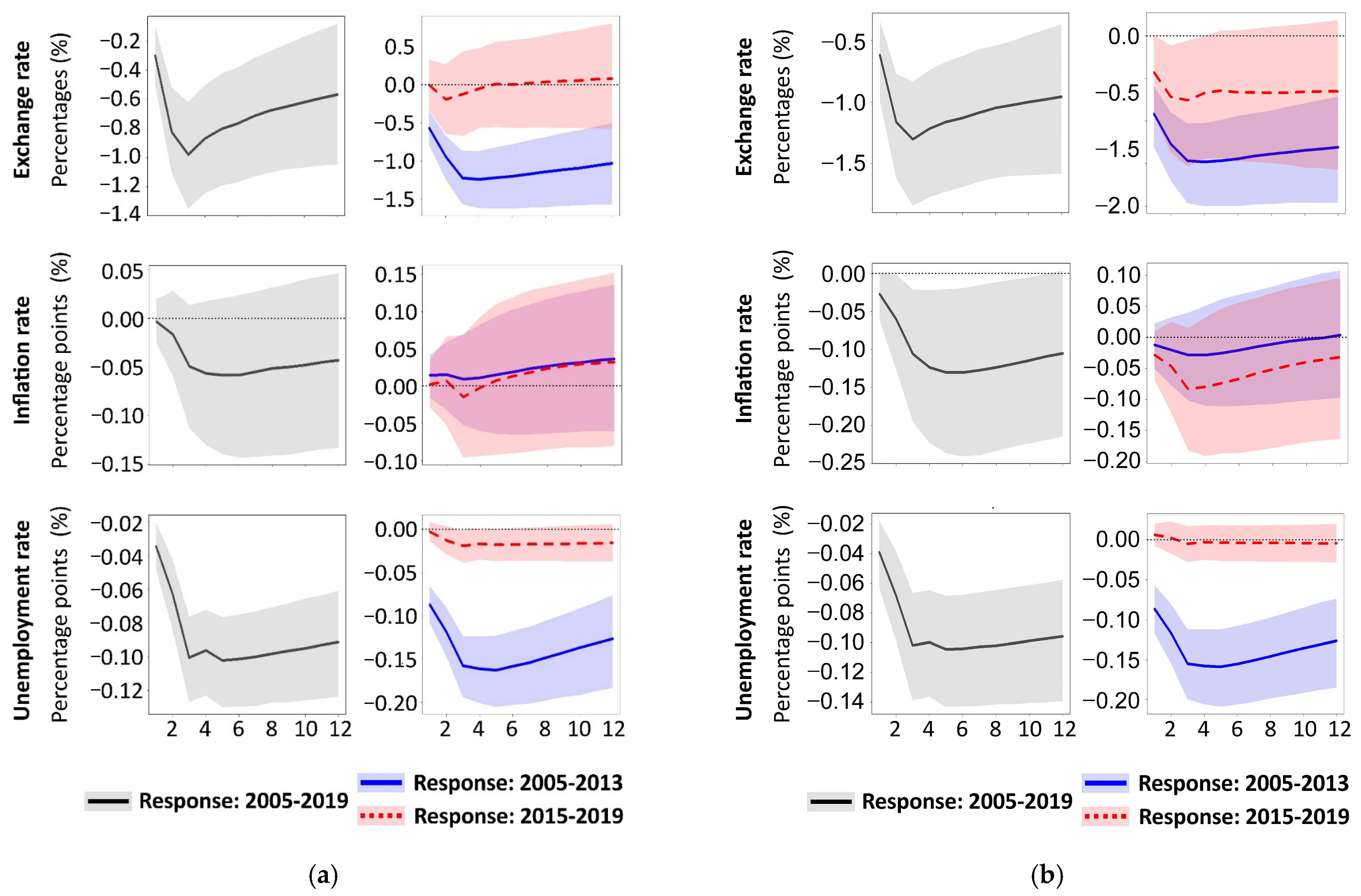
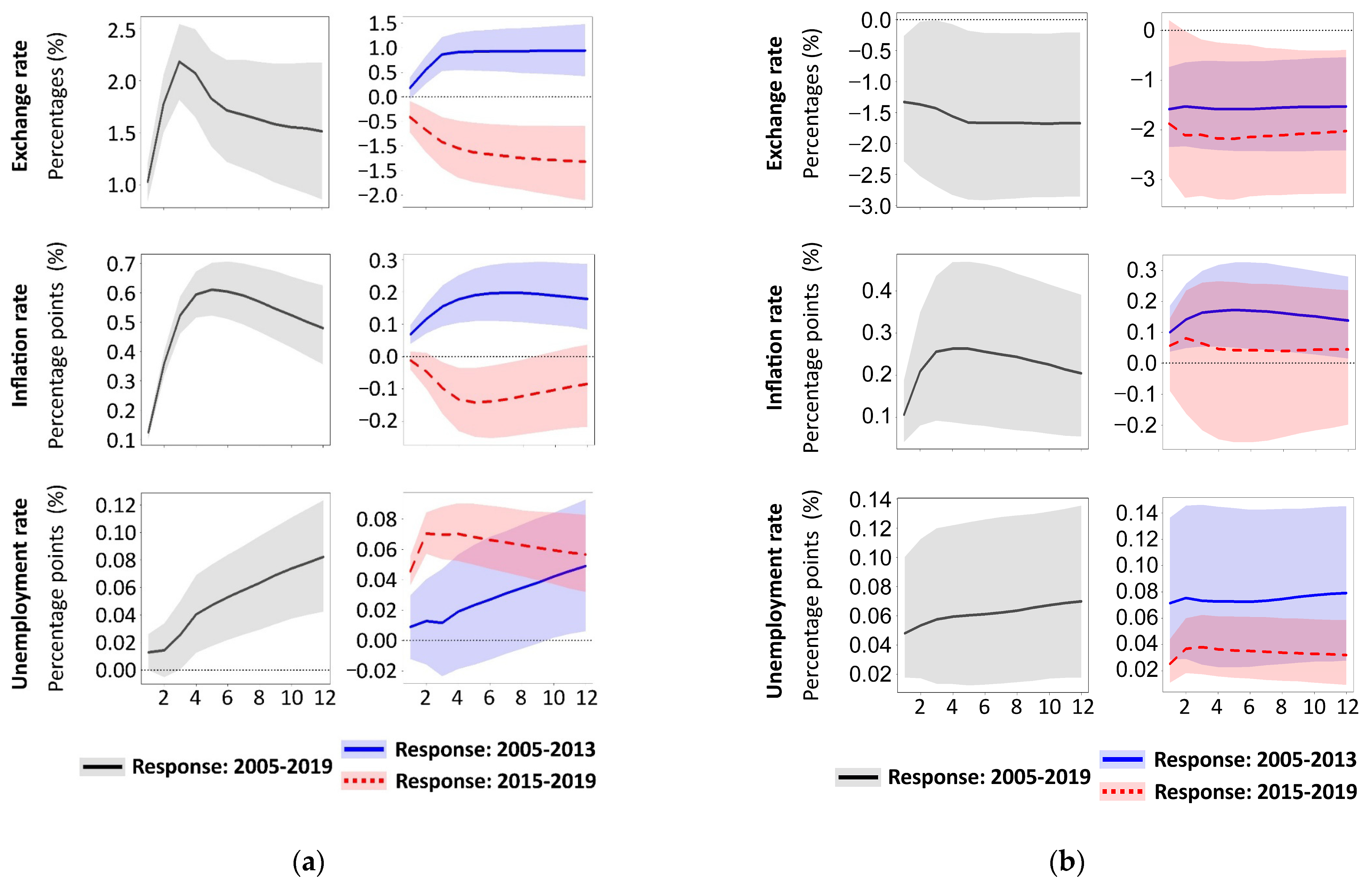
Figure 2 shows the responses of Russian macroeconomic variables to a one-standard-deviation increase in crude oil revenue across models.

The full (2005–2019) model shows that positive oil revenue shocks have a favorable macroeconomic effect on the Russian economy: inflation decreases, the unemployment rate falls, and the national currency appreciates, consistent with the «resource curse» theory. In the pre-2014 model, the pattern’s response is almost the same; however, crude oil revenue amplifies ruble appreciation and unemployment reduction, except for the inflation rate response, which is not significant. Furthermore, after 2014, crude oil revenue has had a lesser influence, as the unemployment rate did not decrease as much as before 2014 in response to positive crude oil revenue shocks. Inflation exhibits no statistically significant response under either identification strategy. The exchange rate response, however, is insignificant under Cholesky identification, but remains significant—albeit smaller compared with the full model—under sign and zero restrictions.

3.3. The Impact of Crude Oil on Russia’s Macroeconomic Policy

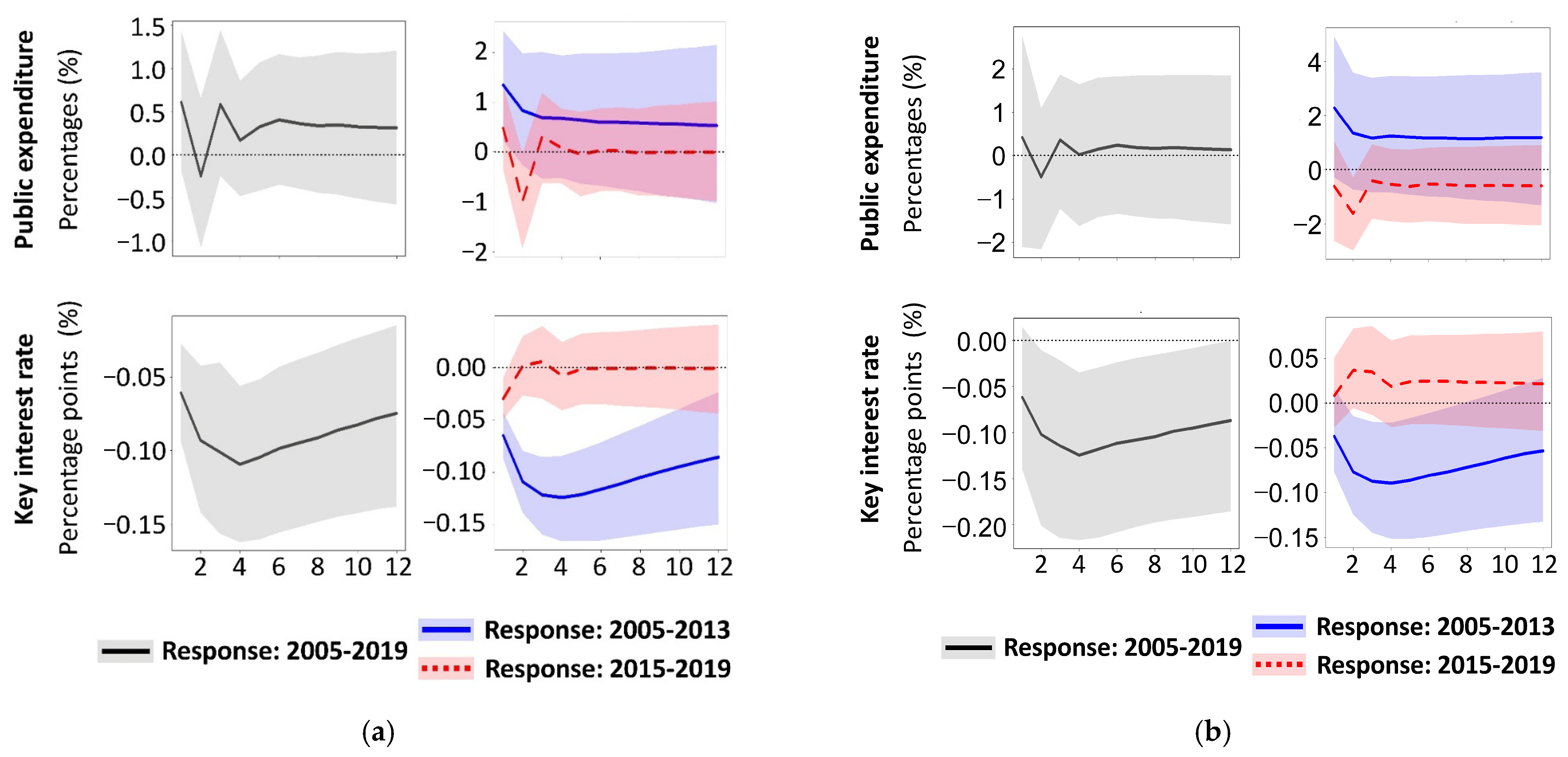
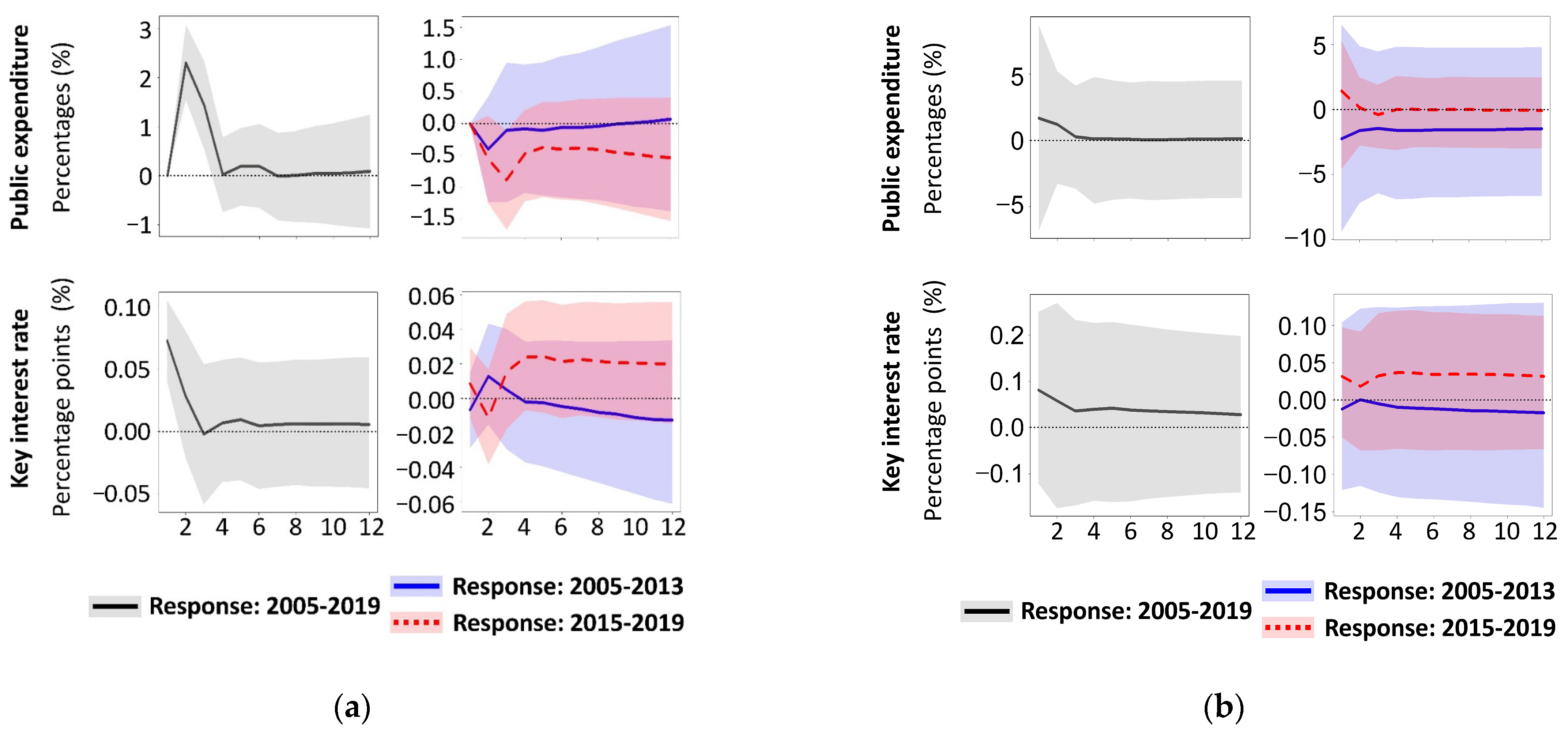
In Figure 3, we analyze the response of the Russian macroeconomic policy variables to a one-standard-deviation increase in crude oil revenue.

The full model shows procyclicality of the key interest rate in response to unexpected positive shocks to crude oil, while the government expenditure response is not significant. Before 2014 the public expenditure response was more expansionary. After 2014, the response shows a short decrease in the first three months with narrower confidence bands. The notable response is that of the key interest rate. Prior to 2014, the response was negative and persistent. Post-2014, the response weakens considerably, being observable only in the first two months under Cholesky identification and exhibiting a more countercyclical pattern under sign and zero restrictions.

3.4. Economic Consequences of Russia’s Macroeconomic Policy Decisions

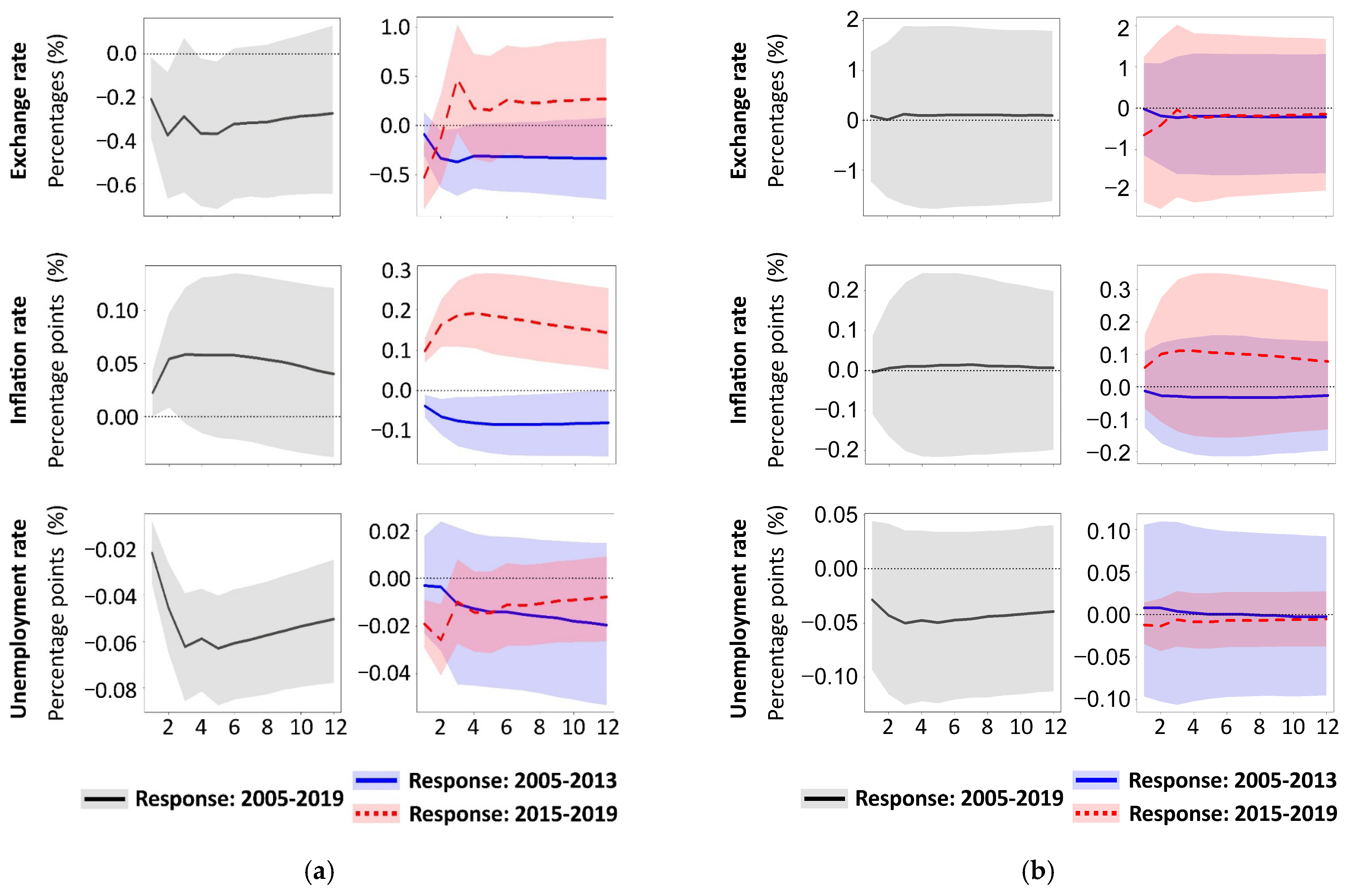
Figure 4 analyzes the transmission effects of a one standard deviation increase in public expenditure on variables of the Russian economy. The lack of statistical significance under sign and zero restrictions suggests that expansionary government expenditure shocks require strict identification. In the absence of precise knowledge of the true data-generating process, imposing directional restrictions may be unwarranted. Consequently, we focus on the Cholesky factorization results, which exhibit statistical significance.

The full model indicates that a positive shock to government expenditure leads to an appreciation of the exchange rate and a reduction in the unemployment rate. However, such expenditure shocks also exhibit a pro-inflationary effect.

However, positive shocks to government expenditure exhibit an anti-inflationary character in the pre-2014 model. The national currency appreciates as in the full model, and the unemployment rate response becomes insignificant during the period.

In the post-2014 model, the exchange rate response is mixed: the ruble appreciates at the beginning, then depreciates after three months following the public expenditure shock. The unemployment rate shows a reduction, but of lesser magnitude than in the full model. However, after 2014, the most profound is inflation, which shows significant and persistent growth in response to positive government expenditure shocks.

Figure 5 analyzes the transmission effects of a one-standard-deviation increase in the key interest rate on variables of the Russian economy. In the full BVAR model, an increase in the key interest rate leads to an appreciation of the exchange rate, with a more persistent and statistically significant response over the first three months under Cholesky factorization. In contrast, under sign and zero restrictions, a positive key interest rate shock results in a depreciation of the exchange rate. It is particularly noteworthy that a positive shock to the key interest rate drives inflation to increase. The unemployment rate gradually rises to the end of the period.

In the pre-2014 model, the exchange rate increases and turns to a new positive level under Cholesky factorization identification. By contrast, under sign and zero restriction identification, a positive key interest rate shock leads to an appreciation of the national currency. It is interesting that in the pre-2014 BVAR model, the key rate hikes also show a pro-inflationary effect under both identification strategies, but their magnitude is smaller than in the full model. While the magnitude of the unemployment rate’s response varies across identification strategies, its overall dynamic pattern mirrors that in its respective full model.

After 2014, the pattern of variable responses shifts as the ruble begins to appreciate following positive interest rate shocks. The estimated response of unemployment to positive key interest shocks is sharper and more pronounced under the Cholesky identification scheme than under the scheme using sign and zero restrictions. Furthermore, while a positive shock to the key interest rate curbs inflation under the Cholesky identification, its effect on inflation remains statistically insignificant under the sign and zero restrictions scheme.

In Figure 6, the study additionally analyzes the impulse responses of government spending and the key interest rate to one-standard deviation shocks in one another. The study refers the Cholesky identification results, as the alternative specification with sign and zero restrictions yields insignificant responses.

Following a positive shock to government expenditure, the key interest rate rises sharply and fades away after three months. Moreover, after a key rate-positive shock, government expenditure rises quickly, peaking in the second month. However, in the pre-2014 model, the effect is statistically insignificant, as is the response of the key interest rate to a government expenditure shock. Although after 2014 the government decreases expenditure in response to a key interest rate shock, and the central bank surges rates to support government expenditure expansion.

3.5. Contributions of Shocks to the Variability of Variables

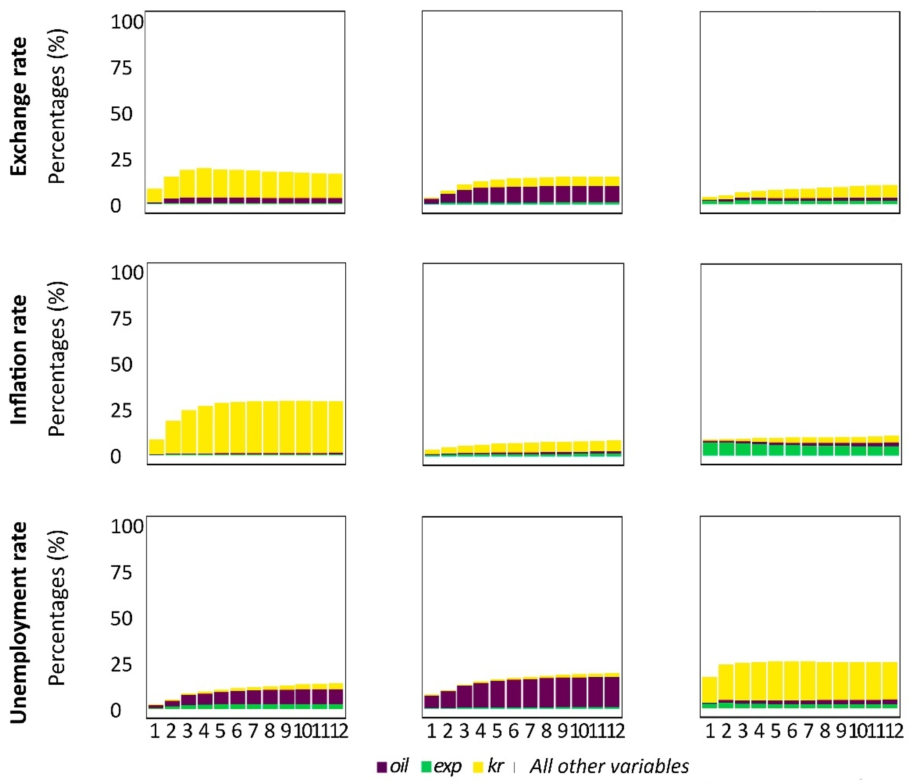
This section uses FEVD to quantify the importance of different structural shocks and to answer three key questions: (i) to what extent do crude oil revenue shocks drive fluctuations in the macroeconomy and macroeconomic policy? (ii) how significant are macroeconomic policy shocks in explaining the variance of macroeconomic indicators? (iii) did the relative contribution of these shocks shift following the 2014 structural break?

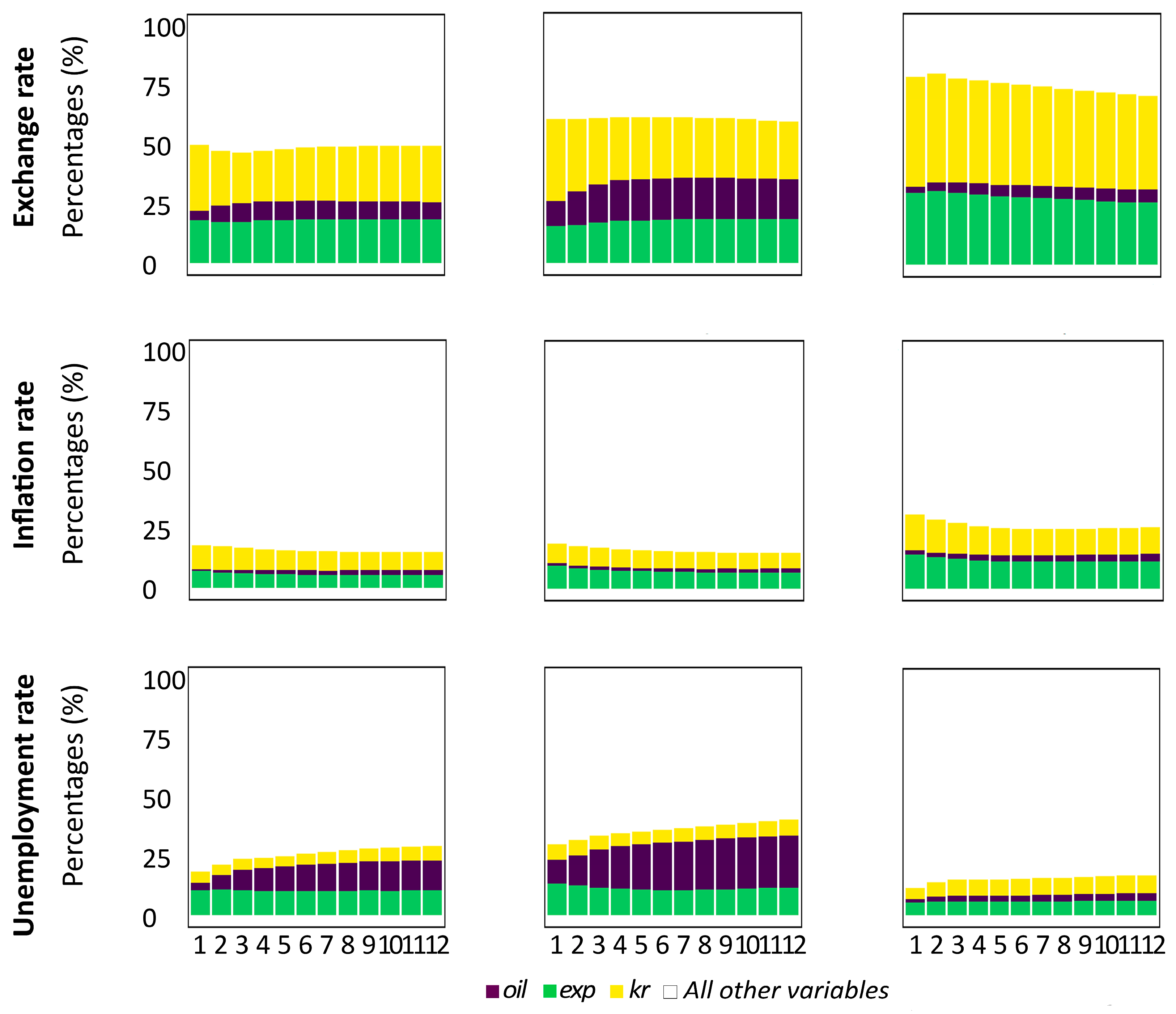
Figure 7 presents the FEVD for macroeconomic and policy variables, highlighting the contributions from crude oil revenue, government expenditure, and the key interest rate.

Table 3. Average forecast error variance decomposition among the full (2005–2019), pre-2014 (2005–2013), and post-2014 (2015–2019) BVAR models. The numbers in parentheses indicate the 68% respective PPBs, based on 90,000 draws after a burn-in of 25,000 and thinning by 13. (The table reports the average aggregate contribution of the variables over the forecast horizon under the Cholesky identification strategy. The disaggregated results for each period are presented in Figure 7 (Cholesky identification) and Figure 8 (sign and zero restrictions). A complete table with contributions for all 12 horizons is available from the authors upon request.).

The Percentage Contribution (%)
	oil	exp	kr	cur	i	u
exp (2005–2019)	0.77 [0.47, 1.23]	95.13 [97.03, 92.37]	1.55 [1.09, 2.16]	0.43 [0.22, 0.77]	1.64 [0.91, 2.62]	0.50 [0.28, 0.85]
exp (2005–2013)	1.27 [0.68, 2.25]	96.54 [98.19, 93.71]	0.56 [0.29, 1.04]	0.16 [0.08, 0.31]	0.87 [0.45, 1.57]	0.60 [0.31, 1.12]
exp (2015–2019)	2.34 [1.63, 3.27]	85.63 [90.19, 80.21]	1.30 [0.79, 2.09]	1.35 [0.76, 2.20]	8.30 [5.94, 10.53]	1.09 [0.69, 1.69]
kr (2005–2019)	1.71 [0.88, 2.81]	0.79 [0.47, 1.27]	94.24 [96.73, 90.85]	1.99 [1.27, 2.74]	0.71 [0.35, 1.32]	0.57 [0.31, 1.01]
kr (2005–2013)	6.90 [4.75, 9.25]	0.78 [0.42, 1.37]	89.16 [93.19, 84.13]	0.15 [0.07, 0.29]	2.32 [1.20, 3.70]	0.69 [0.36, 1.27]
kr (2015–2019)	1.80 [1.12, 2.92]	1.60 [0.94, 2.62]	88.18 [92.72, 82.16]	5.36 [3.64, 7.12]	2.00 [1.01, 3.34]	1.06 [0.56, 1.83]
cur (2005–2019)	2.35 [1.40, 3.50]	0.78 [0.39, 1.35]	13.19 [11.14, 15.02]	82.25 [86.33, 77.65]	0.63 [0.35, 1.07]	0.79 [0.39, 1.41]
cur (2005–2013	7.61 [5.42, 9.65]	1.09 [0.58, 1.90]	3.98 [2.39, 5.77]	85.15 [90.47, 79.06]	1.41 [0.74, 2.32]	0.76 [0.39, 1.31]
cur (2015–2019)	1.47 [0.86, 2.43]	1.96 [1.26, 2.93]	4.59 [2.53, 6.95]	87.60 [92.93, 80.95]	1.43 [0.77, 2.45]	2.95 [1.67, 4.29]
i (2005–2019)	0.56 [0.27, 1.05]	0.62 [0.30, 1.11]	25.21 [23.59, 26.26]	0.55 [0.28, 1.00]	72.18 [75.13, 69.07]	0.88 [0.43, 1.51]
i (2005–2013)	0.92 [0.47, 1.64]	1.33 [0.62, 2.42]	4.72 [2.76, 6.90]	0.52 [0.24, 1.00]	90.81 [95.04, 85.27]	1.70 [0.88, 2.77]
i (2015–2019)	1.40 [0.74, 2.39]	5.95 [3.77, 8.14]	2.50 [1.30, 4.17]	4.18 [2.35, 6.21]	82.98 [90.00, 74.90]	2.99 [1.85, 4.19]
u (2005–2019)	5.92 [4.32, 7.46]	2.34 [1.42, 3.40]	1.81 [0.97, 2.91]	0.76 [0.47, 1.19]	1.02 [0.57, 1.72]	88.16 [92.25, 83.32]
u (2005–2013)	14.00 [11.60, 16.15]	0.77 [0.41, 1.36]	1.16 [0.64, 1.97]	0.95 [0.54, 1.56]	1.54 [0.90, 2.54]	81.58 [85.90, 76.43]
u (2015–2019)	2.09 [1.15, 3.37]	2.31 [1.43, 3.51]	20.11 [17.94, 21.32]	1.57 [0.95, 2.51]	3.96 [2.53, 5.64]	69.96 [76.00, 63.65]

shows the aggregate FEVD for macroeconomic and macropolicy variables. In the FEVD analysis, the forecast error variance for each variable is predominantly explained by its own shocks, a standard result in a BVAR model with a Minnesota prior, where the variable’s own lags largely determine short-term forecasts; however, the study focuses on the combined contribution of crude oil revenue, government expenditure, and key interest rate shocks. (While the main analysis refers to the results shown in Figure 7 and Table 3, the findings based on the sign and zero restrictions are presented separately in Figure 8).

In the full sample, the combined contribution accounts for approximately 16.32% of the exchange rate’s forecast-error variance. Within this, the key interest rate alone accounts for 13.2%. The contribution declines to 12.68% in the pre-2014 period, with crude oil revenue shocks accounting for the largest share at 7.6%. In the post-2014 period, the aggregate explanatory power of these three shocks diminishes further to around 8%.

For inflation, the contribution of crude oil revenue, government expenditure, and key interest rate shocks accounts for roughly 26.4% of the forecast error variance in the full sample, with the key interest rate exerting a powerful influence. This aggregate contribution, however, declines to about 7% in the pre-2014 model (with the key rate accounting for 4.7%). Post-2014, the driver shifts as public expenditure becomes more prominent, explaining roughly 6% of the variance.

The decomposition for unemployment shows the combined contribution of about 10% in the full sample, dominated by crude oil revenue shocks. The dynamics shift markedly across sub-periods. In the pre-2014 model, the aggregate contribution is higher, at approximately 16%, with crude oil revenue accounting for 14% of this share. After 2014, the aggregate contribution rises substantially to 24.5%, but the primary driver changes: the role of crude oil revenues diminishes, while the key interest rate becomes predominant, explaining about 20% of unemployment’s variance.

In summary, the post-2014 period shows reduced oil dependency and a growing importance of fiscal and monetary factors, particularly for inflation and unemployment rate dispersion, suggesting a structural shift in Russia’s macroeconomic transmission mechanisms in 2014.

3.6. Robust Check

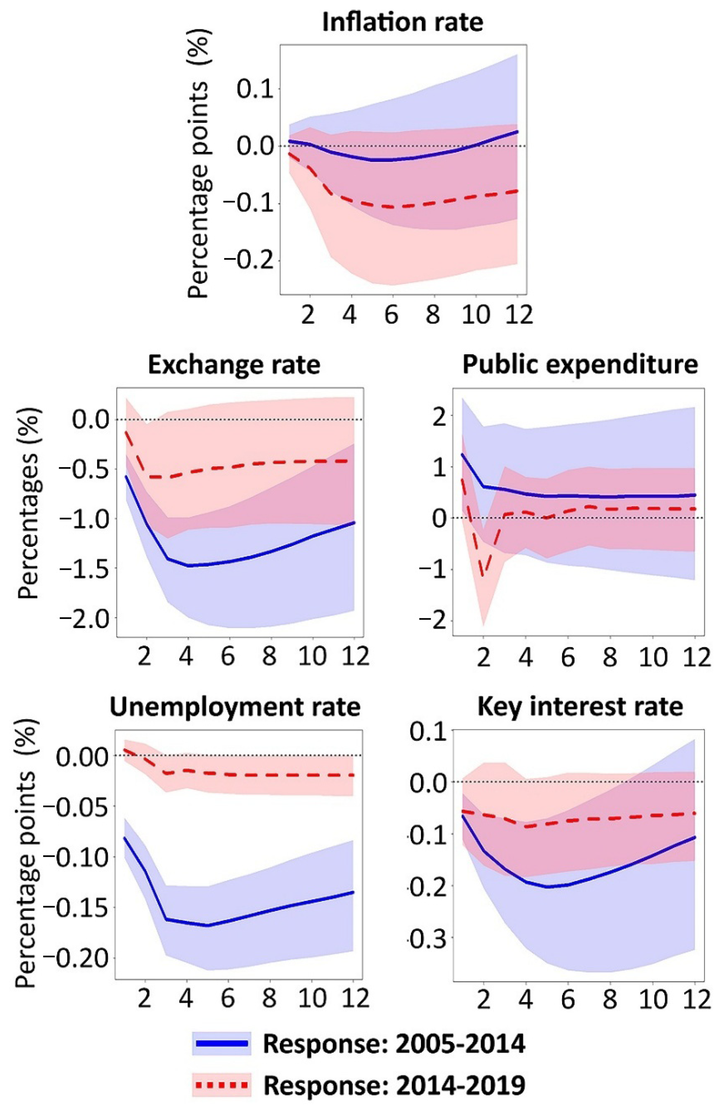
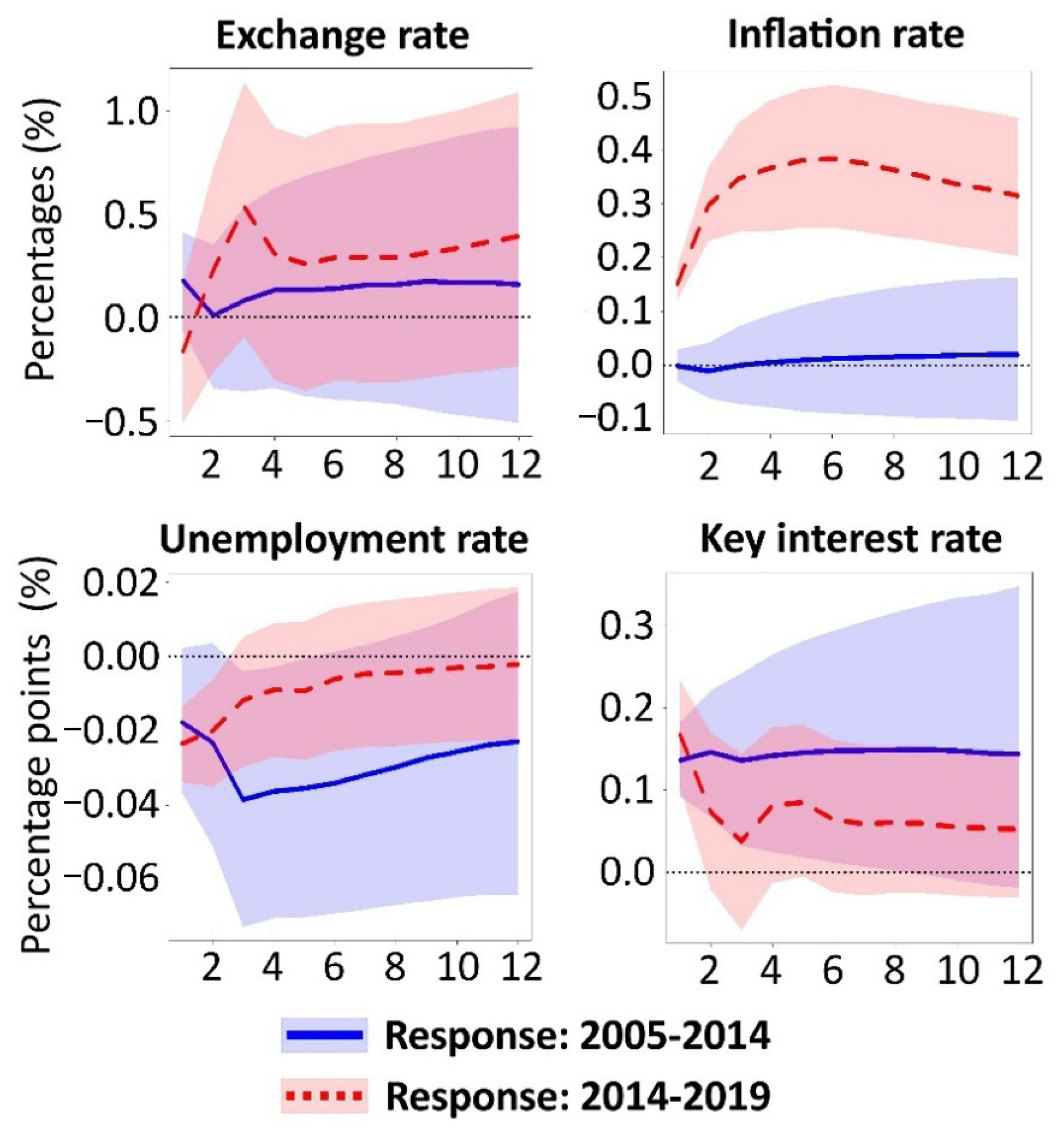
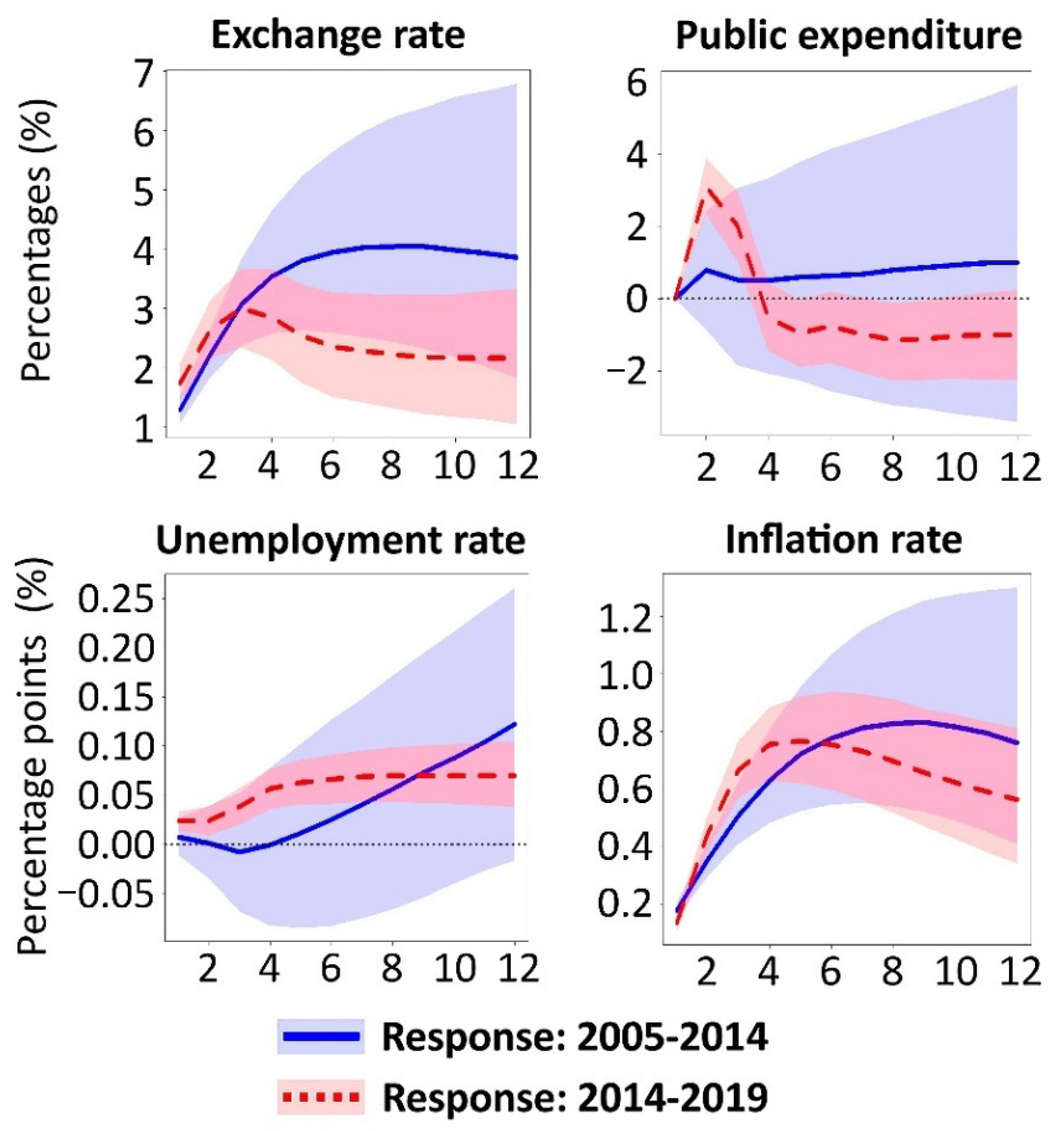
In this section, the study expands the subsample analysis to test whether the structural break alters the results for the periods (1) 2005–2014 and (2) 2014–2019. We also separately conduct a relative analysis for the period prior to 2014, isolating the global financial crisis, and test the BVAR model on the 2009–2013 sample. It is worth noting that all additional models showed poorer chain convergence and a significantly lower marginal likelihood score compared with the base subsample BVAR models that exclude 2014 (see

Table A6. MCMC convergence and numerical stability diagnostics for the full (2005–2019), pre-2014 (2005–2013), and post-2014 (2015–2019) BVAR Models.

Parameters	BVAR (2005–2019)	BVAR (2005–2013)	BVAR (2015–2019)
$\lambda$	0.552	0.344	0.742
$\mu$	0.199	0.321	0.220
$\sigma$	0.071	0.108	0.280
Max autocorrelation of $\lambda$	0.046	0.019	0.022
Accepted draws	0.246	0.289	0.249
ESS	5065.83	5000	4907.643
Coefficients convergence (Gelman–Rubin on three independent chains)	Point $\widehat{R}$ = 1	Point $\widehat{R}$ = 1	Point $\widehat{R}$ = 1
ML	31.295	86.213	84.383

and

Table A7. MCMC Convergence and numerical stability diagnostics for the (2009–2013), (2005–2014), and (2014–2019) BVAR models.

Parameters	BVAR (2009–2013)	BVAR (2005–2014)	BVAR (2014–2019)
$\lambda$	0.315	0.416	0.642
$\mu$	0.689	0.352	0.175
$\sigma$	0.549	0.089	0.087
Max autocorrelation of $\lambda$	0.076	0.0244	0.023
Accepted draws	0.246	0.255	0.314
ESS	3768.533	5011.513	5127.79
Coefficients convergence (Gelman–Rubin on three independent chains)	Point $\widehat{R}$ = 1	Point $\widehat{R}$ = 1	Point $\widehat{R}$ = 1
ML	74.129	19.396	1.139

). Furthermore, the impulse response functions and forecast-error variance decompositions from these additional subsample BVAR models are presented in Appendix B.

3.6.1. 2014–2019 Additional BVAR Model

The effects of oil shocks on government spending and unemployment are consistent with the baseline 2015–2019 BVAR model. In contrast, the key interest rate shows a more procyclical response to oil revenue shocks. Similarly, the ruble appreciates significantly. A notable deviation is observed in inflation, which shows a declining trend in response to oil shocks in the 2014–2019 model specification.

The responses of unemployment, inflation, and the exchange rate to a government spending shock are generally consistent with those from the 2015–2019 BVAR model. Moreover, the 2014–2019 BVAR model reveals a more profound inflationary impact of government spending and a more procyclical response of the key interest rate following a positive government spending shock.

Finally, the responses of all variables to the key interest rate shocks are nearly identical to those in the full 2005–2019 model, which also included the exchange rate and interest rate puzzles—effects similarly observed in developing countries following monetary tightening [32]. Furthermore, Tyunova’s study for Russia, covering the same time frame, confirmed these findings [21].

Therefore, the results largely mirror those of the baseline 2015–2019 and full 2005–2019 BVAR models, with three key exceptions in the robust periods: the key rate is more procyclical, oil shocks are anti-inflationary, and government expenditure shocks are more pro-inflationary.

3.6.2. 2005–2014 Additional BVAR Model

The 2005–2014 BVAR model produces impulse responses to oil revenue shocks that are primarily aligned with the baseline 2005–2013 model, albeit with increased uncertainty, especially regarding the exchange rate and key interest rate response.

Positive government spending shocks lead to a significant decline in both the key interest rate and unemployment. The responses of the exchange rate and inflation are insignificant. We argue that isolating an expenditure expansion shock and the corresponding macroeconomic reactions is statistically difficult for the transformative year of 2014. Consequently, averaging the impulse responses over the entire 2005–2014 period yields an insignificant result; therefore, the result is inconsistent with the 2005–2013 baseline model.

Shocks to the key rate transmit to other macroeconomic indicators in the same way as in the baseline (2005–2013) model.

Therefore, the results of the extended 2005–2014 BVAR model are mainly robust, except for government expenditure shocks, which affect inflation and exchange rates statistically indistinguishably from zero compared with the baseline 2005–2013 model.

3.6.3. 2009–2013 Additional BVAR Model

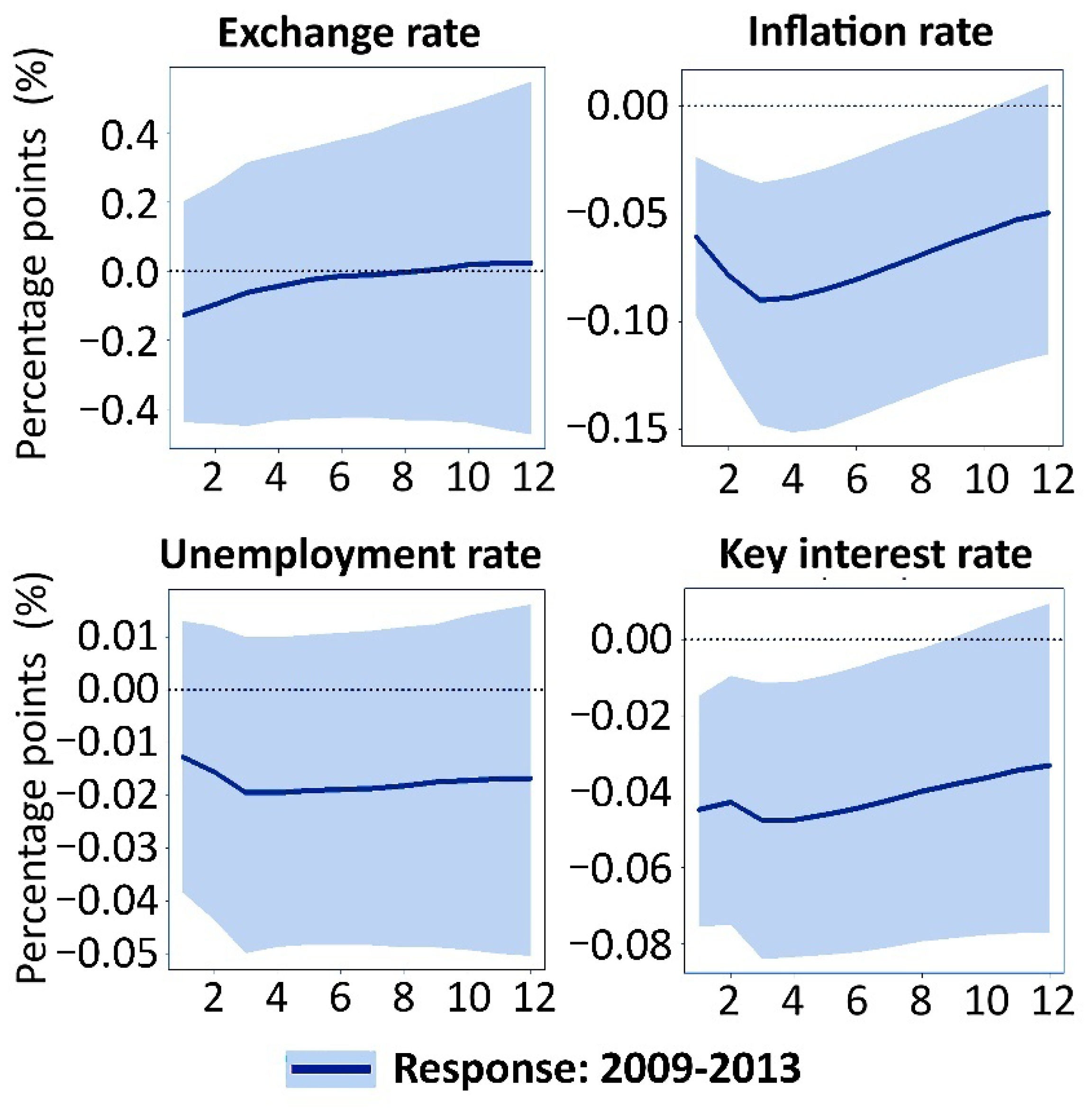
An analysis of data for the 2009–2013 period shows that the unemployment rate rises in response to oil revenue shocks, rather than falling as in the baseline 2005–2013 model. The responses of the key interest rate, exchange rate, and unemployment rate to positive oil shocks are less pronounced than in the baseline BVAR model over the entire 2005–2013 period.

During this same period, the ruble exchange rate is insensitive to positive shocks from government spending. Inflation responds to increases in government spending with a decline, as in the 2005–2013 baseline model. An increase in government spending leads to a clear decline in the key rate.

Furthermore, robust analyses of the 2009–2013 model support the results of the 2005–2013 baseline model, indicating that increases in government spending continue to have an anti-inflationary effect on the economy, while tightening the key rate has a pro-inflationary effect. However, including data from the 2007 crisis in the sample strengthens the measured impact of oil revenues on these macroeconomic indicators in the baseline 2005–2013 model. This result is consistent with Lomonosov, who argued that the impact of oil shocks increases during periods of global economic turmoil [8].

3.6.4. 2005–2013 Additional BVAR Extended Model

This paper reports counterintuitive findings for the pre-2014 period, showing that fiscal expansion reduces inflation while monetary tightening increases it and claims these results are robust, including in an additional subsample from 2009 to 2013.

Given that these findings contradict standard transmission mechanisms, we undertake a stronger validation to rule out omitted variable bias. We introduce an extended comparator specification to the model, designed to incorporate potential biases that might shed light on these anomalous results.

The comparator specification additionally includes Russian retail sales (${ret}_t$), which are seasonally adjusted in billions of rubles, sourced from the Russian Federal State Statistic service. We use its natural logarithm. We added manufacturing production index (${man}_t$) which are seasonally adjusted data from the OECD database (https://stats.oecd.org/viewhtml.aspx?datasetcode=MEI_REAL&lang=en, accessed on 22 January 2026). We also take its natural logarithm to stabilize variance and align its scale with other variables. Finally, we added inflation expectations proxy (${iex}_t$) calculated as the deposit rate (for non-financial organizations, up to one year, excluding demand deposits) minus the key policy rate. This spread serves as a proxy for banking-sector inflation expectations. While ${iex}_t$→ 0 suggests banks anticipate higher inflation and are raising deposit rates accordingly. The deposit rate data were collected from the Central Bank’s official website. (https://cbr.ru/statistics/b_sector/interest_rates_05/, accessed on 22 January 2026). The shocks are identified using a Cholesky factorization, with the following variable order:

$$y_t= \left[\begin{array}{c}\begin{array}{c}\begin{array}{c}{oil}_t\\ {exp}_t\\ {kr}_t\\ {iex}_t\\ {man}_t\\ {ret}_t\end{array}\\ {cur}_t\\ i_t\end{array}\\ u_t\end{array}\right]$$

(11)

The impulse responses of key macroeconomic variables to crude oil revenue, public expenditure, and policy rate shocks are broadly consistent with the baseline model estimates for the pre-2014 period (The IRF results for the extended model are presented in Appendix B (Figure A9, Figure A10 and Figure A11)). However, a positive government expenditure shock is associated with high and persistent inflation expectations and a decline in the manufacturing index. Similarly, hikes in the key policy rate reduces inflation expectations, retail sales, and manufacturing output. Crucially, the core counterintuitive finding remains: policy rate increases continue to exhibit a positive effect on inflation, while government spending expansions appear to be disinflationary.

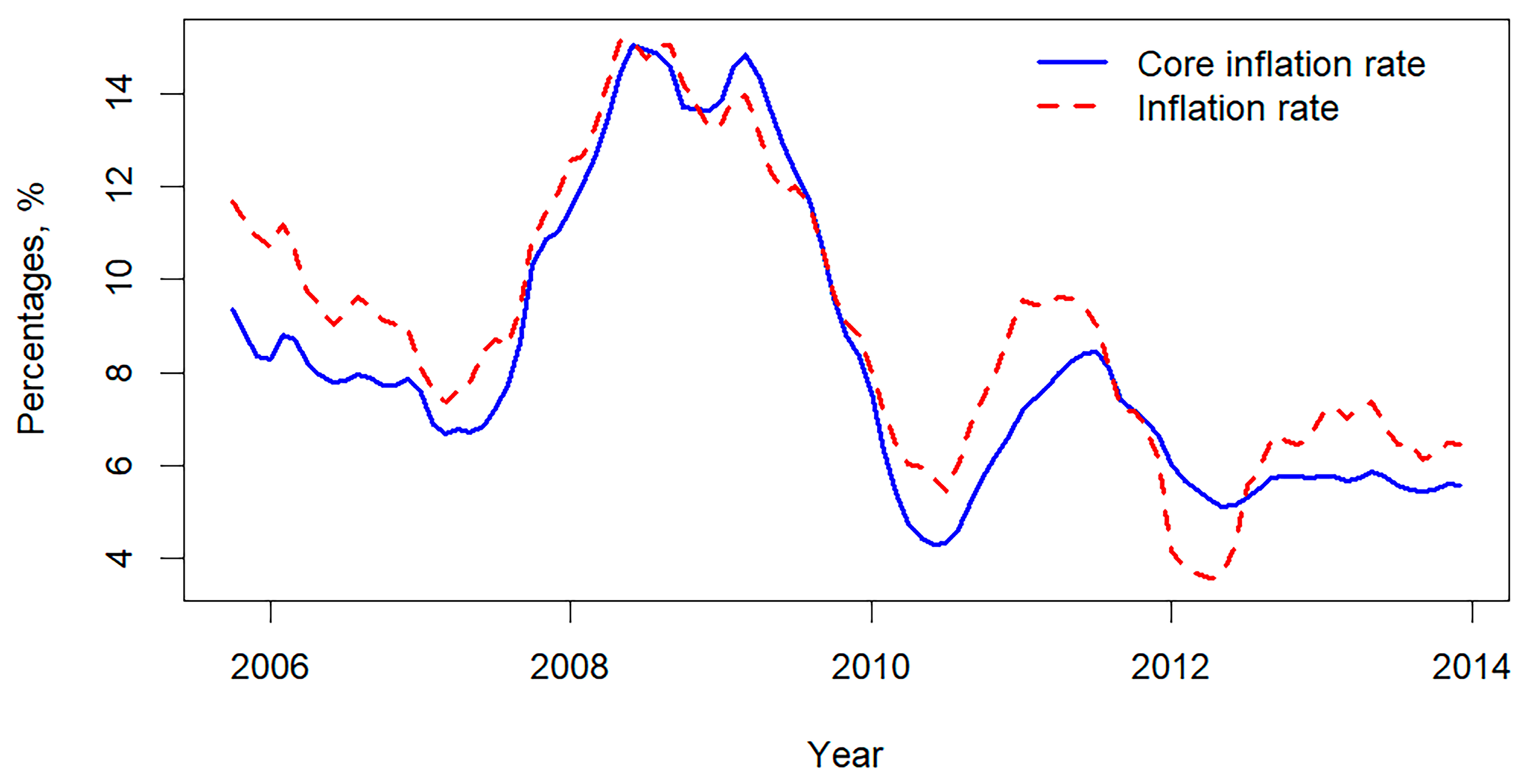
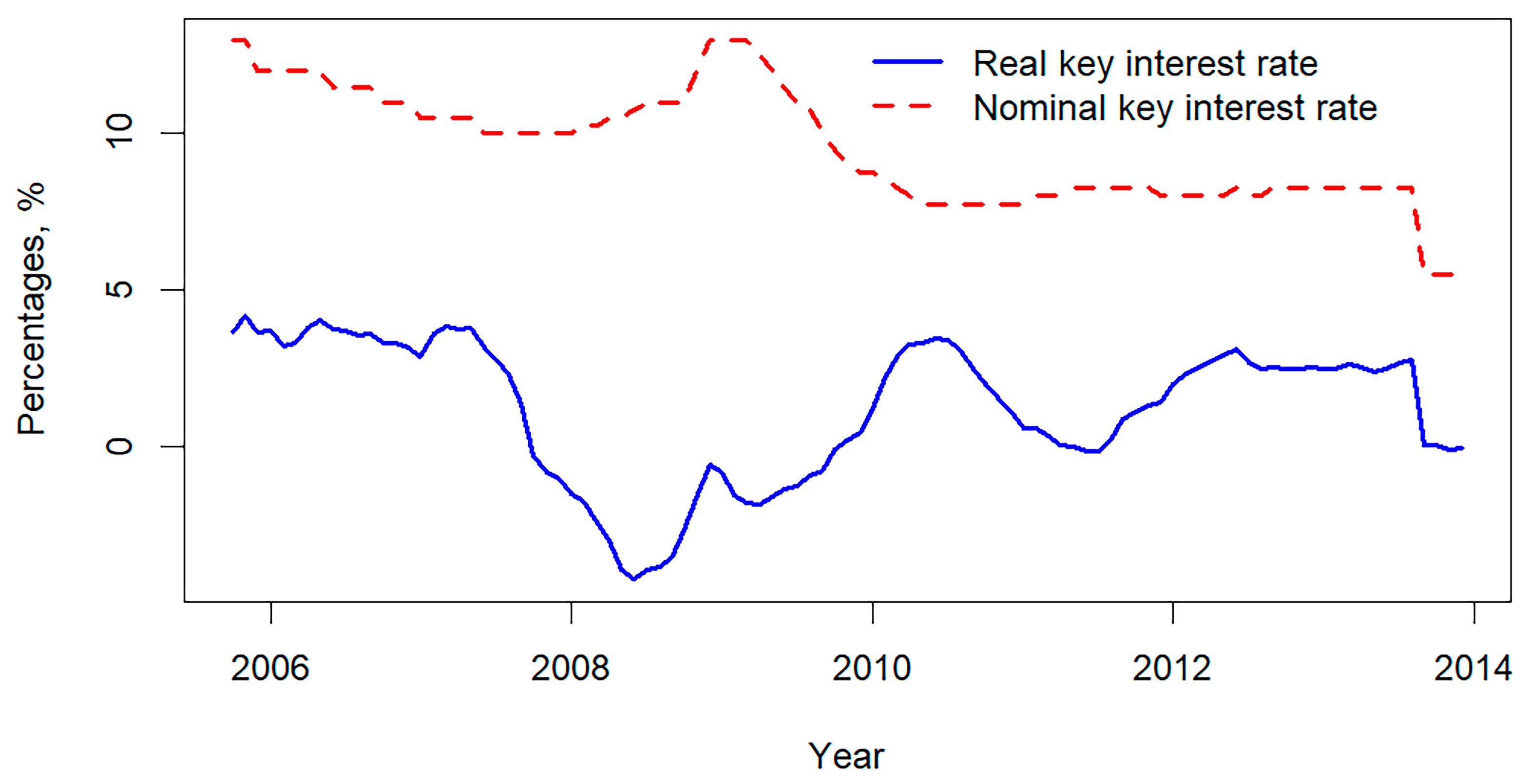
To assess the robustness of the transmission mechanism and to distinguish between nominal policy actions and the realized monetary stance, we replace headline inflation with core inflation (see Figure 9) and the nominal policy rate with the ex post real policy rate (see Figure 10). Importantly, the ex post real policy rate is not interpreted as a structural monetary policy instrument but rather as a measure of realized monetary tightness that incorporates inflation outcomes.

The results indicate that, in the pre-2014 period, innovations to the ex post real policy rate remain procyclical with respect to positive crude oil revenue shocks, suggesting that commodity-driven expansions are not systematically offset by effective real monetary tightening. At the same time, core inflation exhibits a more pronounced and persistent decline following positive crude oil revenue shocks.

In contrast, the response of core inflation to government expenditure shocks is not statistically significant, while innovations associated with higher realized real policy rates are followed by a statistically significant decline in inflation. This pattern suggests that inflation reduction occurs primarily when nominal policy actions translate into effective real monetary restraint, highlighting the role of inflation dynamics and ex post realizations in shaping the strength of monetary transmission.

These findings imply that the government spending shock’s disinflationary effect, evident in headline inflation, vanishes for core inflation. This suggests the transmission operates primarily through the exchange rate channel. Finally, the specification using the nominal policy rate likely captures a typical price puzzle. When the real policy rate is employed instead, the puzzle disappears, and a standard monetary transmission mechanism is restored: a monetary tightening effectively reduces inflation.

4. Discussion

The evolution of the Russian economy since 2014 has demonstrated substantial shifts.

• After 2014, fiscal expansion shifted from an anti-inflationary tool to an inflationary driver and a depreciating force on the national currency.

Before 2014, the anti-inflationary nature of expanding government expenditure, which also had appreciated the national currency, was revealed. Such exchange rate and price puzzles are rare for fiscal expansion. Therefore, we hypothesize that the pre-2014 government expenditure shock may have been interpreted as a signal of improved fiscal sustainability, especially when combined with external financing. This perception could have induced capital inflows and led to currency appreciation. A stronger currency would hurt the price competitiveness of the domestic manufacturing sector and increased imports leading to lower headline inflation. Conversely, inflation expectations of the banking sector could have risen because economic agents might have extrapolated the increase in government spending as potentially inflationary.

Perhaps after 2014, government spending overheated aggregate demand, leading to inflation. Consequently, the significant decline in oil revenues after 2014 and the resulting budget deficit were financed primarily through domestic borrowing and monetary expansion.

• After 2014, the monetary policy’s tight stance became explicitly anti-inflationary.

Although hikes in the key policy rate lowered banking sector inflation expectations before 2014, their overall disinflationary effect may be attributed to a broader information shock. The central bank’s reactive use of the key rate—adjusting it after crises emerged—signaled a failure of monetary policy. This approach may fuel panic, leading to immediate price surges as the market prices in future risks. It is possible that the ruble devaluation in response to monetary policy tightening had financial consequences, as did the key rate increase. This result aligns with prior literature documenting adverse effects of monetary tightening in emerging economies. For instance, the “exchange rate puzzle”—where interest rate hikes lead to currency depreciation—has been observed in 73% of 72 developing countries [32]. The dominant explanation is that in such economies, underdeveloped financial markets amplify the contractionary effect of higher rates on the real sector. This domestic slowdown undermines currency confidence, and the resulting negative impact outweighs the potential stabilizing inflow of foreign capital. Consequently, the net effect of monetary tightening can be a depreciation of the national currency.

Ultimately, the result is robust across different specifications and is unlikely to be a technical or identification artifact, as similar findings are reported in other studies [21,33]. Finally, the traditional monetary transmission channel remains valid, as the analysis of a positive ex-post real key interest rate shock shows a decrease in inflation.

After 2014, the central bank began operating more transparently, switching to an inflation-targeting policy. The signal sent by rate hikes has shifted. Rather than being interpreted as a desperate reaction to lost control, the monetary tightening became seen as a credible, preemptive measure to maintain price stability. However, the response to a key interest rate shock was not statistically significant under the alternative (sign and zero restrictions) strategy, which left the inflation response unrestricted. This insignificance may imply that the effect of interest rates on inflation is heterogeneous and varies over time.

• Post-2014, fiscal policy became increasingly constrained by the central bank’s more dominant inflation targeting regime.

After 2014, the dominance of the key rate and inflation targeting was firmly established. A new hierarchy of policy instruments emerged: fiscal expansion triggered an automatic monetary tightening, which in turn constrained budgetary ambitions. As a result of the structural transformations of Russia’s macroeconomic policy after 2014, and by analyzing the Russian economy’s oil dependence before and after 2014, the research came to the conclusion that:

• Russia’s economic dependence on oil diminished after 2014, as evidenced by the exchange rate of its domestic currency and the unemployment rate.

Notably, the IRF in the pre-2014 period shows amplification of crude oil’s impact on national currency appreciation and a reduction in the unemployment rate. In contrast, the effect of crude oil decreases after 2014. The FEVD analysis also points to a pronounced decline after 2014 in the role of crude oil shocks in explaining the variance in the exchange rate and the unemployment rate, alongside a growing influence of macroeconomic policy on these indicators. The notion contributes to the following literature [1,2,3,4,5,6,7]. The analysis also finds a reduced influence of crude oil revenues on macroeconomic indicators during the 2009–2013 period, when the structural break from the 2007 financial crisis is excluded, consistent with [8].

• Macroeconomic policy (government expenditure and key interest rate) shifted from procyclical to countercyclical in response to oil revenue shocks after 2014.

The macroeconomic policy framework has transformed. During 2005–2013, the central bank pursued a more procyclical monetary policy in response to oil revenue growth, likely aiming to mitigate ruble appreciation. While this approach may have stimulated aggregate demand and fostered economic expansion, it also exacerbated the adverse effects of the subsequent oil revenue windfalls, making the Economy more oil-dependent. Following 2014, however, sensitivity to crude oil shocks declined markedly, with the magnitude and duration of the reactions substantially reduced. This decline in key interest rate dependence is concurrent with the implementation of inflation targeting, supporting the theoretical frameworks of Drygalla [3] and Idrisov [7], and aligning with the practical findings of Tyunova [21]. Government expenditure followed a similar pattern, with a countercyclical response to crude oil positive shocks. Finally, the results contribute to the understanding of the cyclical nature of macroeconomic policy in the following literature [6,17,18,20,21,22,33].

Thus, the analysis confirms a statistically significant difference in how oil revenues, government spending, and the key interest rate affect the economy before (2005–2013) and after (2015–2019) the structural break in 2014. Crucially, the superiority of splitting the 2005–2019 period into pre- and post-2014 intervals is supported by the Bayesian model comparison metric, the marginal likelihood, which favors the partitioned specification (Table A6). In addition, the full-sample model fails to capture the distinct structural differences revealed in the subsamples, particularly in the impact of crude oil revenue and the transmission of policy shocks from government expenditure and the key interest rate. The comparative analysis shows that these factors had fundamentally different effects on core Russian macroeconomic indicators—the exchange rate, inflation, and unemployment rates—before and after 2014.

5. Conclusions

This paper reconsiders two key areas using structural Bayesian vector autoregression subsample models: potential differences in macroeconomic policy and the effects of crude oil revenue shocks on the Russian macroeconomy. We analyzed and compared six samples spanning from 2005 to 2019, accounting for the policy structural shift in 2014 in the Russian context. The study documented macroeconomic policy as procyclical before and more countercyclical after 2014. The paper found an increased role for fiscal and monetary factors and a reduced influence of crude oil revenues after 2014. Using the Russian Federation as a pivotal case study, it demonstrates that an inflation-targeting regime is a viable strategy for commodity-reliant nations seeking to reduce oil dependence and insulate their domestic economies. Moreover, fiscal policymakers began to give greater consideration to the institutional objective of monetary policy, namely inflation targeting. Thus, our key recommendation for further insulating the economy from oil shocks is to strengthen institutional quality and coordination between monetary and fiscal authorities. The core objective of this framework should be to uphold and periodically reassess the fiscal rule as the primary buffer against oil revenue volatility, thereby safeguarding the Central Bank’s ability to focus on price stability. A critical element is aligning fiscal expansion goals with the monetary policy stance to avoid conflicting stimuli, as exemplified by the post-2022 experience. During that period, expansive fiscal measures, insufficiently offset by monetary tightening, contributed to inflationary pressures, ultimately necessitating sharper interest rate hikes and currency appreciation—a painful adjustment for a weakened economy. Therefore, in an era of constrained external financing, close cooperation on public debt management and systemic liquidity is essential to prevent fiscal actions from translating into excessive inflationary pressure.

Notably, this study proves that the linear full-sample model fails to capture divergent responses in macroeconomic variables, while including the 2014 structural break data reduces interpretability. These findings underscore the need to account for structural breaks in BVAR models when analyzing macroeconomic policy in the Russian context.

While this study provides a comparative analysis of transmission mechanisms, several avenues for future research could extend and refine its findings. First, our linear framework does not capture potential non-linearities in how oil dependence shapes Russia’s economic and policy dynamics; a non-linear approach could better identify structural shocks and heterogeneous effects. Second, certain counterintuitive results in the pre-2014 period—such as fiscal expansion reducing inflation and monetary tightening increasing it—warrant further investigation, especially since similar paradoxical effects have been documented in other studies on emerging countries. Third, alternative identification strategies could be employed to explore different nuances of macroeconomic policy dynamics. Finally, although we confirm the challenge of isolating crude oil tax revenue shocks (which may originate from fiscal, production, or price channels), future work could pursue a decomposition of oil revenues to achieve purer identification. We encourage further research in these directions to build upon the present analysis.

References

1. Alekhina, V.; Yoshino, N. Exogeneity of World Oil Prices to the Russian Federation’s Economy and Monetary Policy. Eurasian Econ. Rev. 2019, 9, 531–555. [Google Scholar] [CrossRef]
2. Nyangarika, A.M.; Tang, B. Influence oil price towards economic indicators in Russia. In Proceedings of the IOP Conference Series: Earth and Environmental Science, Xiamen, China, 3–5 September 2018; Volume 192, p. 012066. [Google Scholar] [CrossRef]
3. Drygalla, A. Monetary policy in an oil-dependent economy in the presence of multiple shocks. Rev. World Econ. 2023, 159, 185–214. [Google Scholar] [CrossRef]
4. Ito, K. Dutch disease and Russia. Int. Econ. 2017, 151, 66–70. [Google Scholar] [CrossRef]
5. Balashova, S.; Serletis, A. Oil Price Shocks and the Russian Economy. J. Econ. Asymmetries 2020, 21, e00148. [Google Scholar] [CrossRef]
6. Benedictow, A.; Fjærtoft, D.; Løfsnæs, O. Oil Dependency of the Russian Economy: An Econometric Analysis. Econ. Model. 2013, 32, 400–428. [Google Scholar] [CrossRef]
7. Idrisov, G.; Kazakova, M.; Polbin, A. A theoretical interpretation of the oil prices impact on economic growth in contemporary Russia. Russ. J. Econ. 2015, 1, 257–272. [Google Scholar] [CrossRef]
8. Lomonosov, D.; Polbin, A.; Fokin, N. The Impact of Global Economic Activity, Oil Supply and Speculative Oil Shocks on the Russian Economy. HSE Econ. J. 2021, 25, 227–262. [Google Scholar] [CrossRef]
9. Wang, K.H.; Liu, L.; Li, X.; Oana-Ramona, L. Do oil price shocks drive unemployment? Evidence from Russia and Canada. Energy 2022, 253, 124107. [Google Scholar] [CrossRef]
10. Su, C.W.; Qin, M.; Tao, R.; Umar, M. Does oil price really matter for the wage arrears in Russia? Energy 2020, 208, 118350. [Google Scholar] [CrossRef]
11. Yang, J.; Rizvi, S.K.A.; Tan, Z.; Umar, M.; Koondhar, M.A. The Competing Role of Natural Gas and Oil as Fossil Fuel and the Non-Linear Dynamics of Resource Curse in Russia. Resour. Policy 2021, 72, 102100. [Google Scholar] [CrossRef]
12. Lopez-Murphy, P.; Villafuerte, M. Fiscal policy in oil producing countries during the recent oil price cycle. Int. Monet. Fund 2010, 2010, 1–24. [Google Scholar] [CrossRef]
13. Erbil, N. Is fiscal policy procyclical in developing oil-producing countries? Int. Monet. Fund 2011, 2011, 1–32. [Google Scholar] [CrossRef]
14. Cologni, A.; Manera, M. Exogenous Oil Shocks, Fiscal Policies and Sector Reallocations in Oil Producing Countries. Energy Econ. 2013, 35, 42–57. [Google Scholar] [CrossRef]
15. Ayivodji, G.F.; Essl, S.M.; Galego, M.A.; Matta, S.N.; Richaud, C.M. Fiscal Vulnerabilities in Commodity Exporting Countries and the Role of Fiscal Policy; MTI Discussion Paper; World Bank: Washington, DC, USA, 2019; Volume 1. [Google Scholar]
16. Coutinho, L.; Georgiou, D.; Heracleous, M.; Michaelides, A.; Tsani, S. Limiting Fiscal Procyclicality: Evidence from Resource-Dependent Countries. Econ. Model. 2022, 106, 105700. [Google Scholar] [CrossRef]
17. Sohag, K.; Sokhanvar, A.; Belyaeva, Z.; Mirnezami, S.R. Hydrocarbon prices shocks, fiscal stability and consolidation: Evidence from Russian Federation. Resour. Policy 2022, 76, 102635. [Google Scholar] [CrossRef]
18. Gurvich, E.; Vakulenko, E.; Krivenko, P. Cyclicality of Fiscal Policy in Oil-Producing Countries. Probl. Econ. Transit. 2009, 52, 24–53. [Google Scholar] [CrossRef]
19. Tuzova, Y.; Qayum, F. Global oil glut and sanctions: The impact on Putin’s Russia. Energy Policy 2016, 90, 140–151. [Google Scholar] [CrossRef]
20. Çiçekçi, C.; Gaygısız, E. Procyclicality of fiscal policy in oil-rich countries: Roles of resource funds and institutional quality. Resour. Policy 2023, 85, 103675. [Google Scholar] [CrossRef]
21. Tyunova, M. The Impact of Modern Monetary Policy on the Dynamics of Key Macroeconomic Indicators in Russia. Ph.D. Dissertation, Lomonosov Moscow State University, Moscow, Russia, 17 December 2019. [Google Scholar]
22. Jin, H.; Xiong, C. Fiscal Stress and Monetary Policy Stance in Oil-Exporting Countries. J. Int. Money Financ. 2021, 111, 102302. [Google Scholar] [CrossRef]
23. Yildirim, Z.; Guloglu, H. Macro-financial transmission of global oil shocks to BRIC countries—International financial (uncertainty) conditions matter. Energy 2024, 306, 132297. [Google Scholar] [CrossRef]
24. The Central bank of Russian Federation. Available online: https://cbr.ru/content/document/file/87372/on_2015(2016-2017).pdf (accessed on 11 January 2026).
25. Giannone, D.; Lenza, M.; Primiceri, G.E. Prior Selection for Vector Autoregressions. Rev. Econ. Stat. 2015, 97, 436–451. [Google Scholar] [CrossRef]
26. Kuschnig, N.; Lukas, V. BVAR: Bayesian Vector Autoregressions with Hierarchical Prior Selection in R. J. Stat. Softw. 2021, 100, 1–27. [Google Scholar] [CrossRef]
27. Kilian, L.; Lütkepohl, H. Bayesian VAR Analysis. In Structural Vector Autoregressive Analysis; Cambridge University Press: Cambridge, UK, 2017. [Google Scholar] [CrossRef]
28. Sims, C.A.; Stock, J.H.; Watson, M.W. Inference in linear time series models with some unit roots. Econom. J. Econom. Soc. 1990, 58, 113–144. [Google Scholar] [CrossRef]
29. Litterman, R.B. Forecasting with Bayesian vector autoregressions—Five years of experience. J. Bus. Econ. Stat. 1986, 4, 25–38. [Google Scholar] [CrossRef]
30. Knotek, E.S., II; Zaman, S. Asymmetric responses of consumer expenditure to energy prices: A threshold VAR approach. Energy Econ. 2021, 95, 105127. [Google Scholar] [CrossRef]
31. Sims, C.; Zha, T. Bayesian Methods for Dynamic Multivariate Models. Int. Econ. Rev. 1998, 39, 949–968. [Google Scholar] [CrossRef]
32. Hnatkovska, V.; Lahiri, A.; Vegh, C.A. The exchange rate response to monetary policy innovations. Am. Econ. J. Macroecon. 2016, 8, 137–181. [Google Scholar] [CrossRef]
33. Tyunova, M. The Impact of Central Bank Policy on Production Dynamics and Inflation in Russia. Audit. Financ. Anal. 2018, 2, 185–195. Available online: https://istina.ipmnet.ru/publications/article/152182811/ (accessed on 11 January 2026).
Figure 1. The cyclical dynamics of key macroeconomic indicators and policy variables in Russia. Note: the cyclical components were extracted from quarterly data using the Hodrick–Prescott (HP) filter.
Systems 14 00133 g001
Figure 2. The comparison of macroeconomic variable responses to a positive oil revenue shock: (a) Cholesky factorization identification strategy; (b) sign and zero restrictions identification strategy. The grey line represents the variable responses during 2005–2019, the blue line represents the variable responses during 2005–2013, while the red line corresponds to 2015–2019. The shaded regions indicate the 68% respective PPBs, based on 90,000 draws after a burn-in of 25,000 and thinning by 13.
Systems 14 00133 g002
Figure 3. The comparison of macroeconomic policy variable responses to a positive oil revenue shock: (a) Cholesky factorization identification strategy; (b) sign and zero restrictions identification strategy. The grey line represents the variable responses during 2005–2019, the blue line represents the variable responses during 2005–2013, while the red line corresponds to 2015–2019. The shaded regions indicate the 68% respective PPBs, based on 90,000 draws after a burn-in of 25,000 and thinning by 13.
Systems 14 00133 g003
Figure 4. Comparison of macroeconomic variable responses to a public expenditure positive shock: (a) Cholesky factorization identification strategy; (b) sign and zero restrictions identification strategy. The grey line represents the variable responses during 2005–2019, the blue line represents the variable responses during 2005–2013, while the red line corresponds to 2015–2019. The shaded regions indicate the 68% respective PPBs, based on 90,000 draws after a burn-in of 25,000 and thinning by 13.
Systems 14 00133 g004
Figure 5. Comparison of macroeconomic variable responses to a key policy interest rate positive shock: (a) Cholesky factorization identification strategy; (b) sign and zero restrictions identification strategy. The grey line represents the variable responses during 2005–2019, the blue line represents the variable responses during 2005–2013, while the red line corresponds to 2015–2019. The shaded regions indicate the 68% respective PPBs, based on 90,000 draws after a burn-in of 25,000 and thinning by 13.
Systems 14 00133 g005
Figure 6. Comparison of the impulse responses of government spending and the key interest rate to one-standard-deviation positive shocks in one another: (a) Cholesky factorization identification strategy; (b) sign and zero restrictions identification strategy. The grey line represents the variable responses during 2005–2019, the blue line represents the variable responses during 2005–2013, while the red line corresponds to 2015–2019. The shaded regions indicate the 68% respective PPBs, based on 90,000 draws after a burn-in of 25,000 and thinning by 13.
Systems 14 00133 g006
Figure 7. Decomposition of forecast error variance under Cholesky factorization identification strategy. (Left) full model (2005–2019), (middle) pre-2014 sub-period model (2005–2013), (right) post-2014 sub-period model (2015–2019). Cholesky factorization identification strategy.
Systems 14 00133 g007
Figure 8. Decomposition of forecast error variance under sign and zero identification strategy. (Left) full model (2005–2019), (middle) pre-2014 sub-period model (2005–2013), (right) post-2014 sub-period model (2015–2019).
Systems 14 00133 g008
Figure 9. A comparison of the dynamics of headline inflation and core inflation between 2005 and 2013.
Systems 14 00133 g009
Figure 10. A comparison of the dynamics of nominal key interest rate and real key interest rate between 2005 and 2013. (The ex post real policy rate is approximated as the nominal key interest rate minus core inflation).
Systems 14 00133 g010