The Thermodynamic Cliff: Pricing the Climate Adaptation Gap in Digital Infrastructure

Abstract

Conventional climate-risk frameworks, ranging from ESG ratings to Integrated Assessment Models (IAMs), systematically underestimate physical risks by overlooking the non-linear physics that govern infrastructure failure. These top-down models perceive climate change as a manageable operational expense, thereby obscuring the substantial capital requirements necessary to sustain system reliability as global temperatures escalate. This study proposes a physics-first framework to quantify the “Adaptation Gap”—a measurable, unaccounted-for capital liability representing the additional cost needed to upgrade assets to maintain fault tolerance. Within this specific geographic and asset context, it has been determined that restoring fault tolerance for new equipment necessitates a 19.7% (95% CI: 16.5–22.9%) increase in capital expenditure, which increases the Adaptation Gap to 28.7% for typical in-service assets, potentially increasing the true cost for aging assets to between 25% and 30%. Although the quantitative findings are specific to the case study, the methodological framework—assessed as superior to traditional risk metrics—is designed for global application in pricing the Adaptation Gap across all infrastructure sectors with thermal constraints. Our methodology provides a blueprint for establishing a new standard of climate-adjusted valuation, transforming abstract physical risks into a tangible, auditable capital liability.

1. Introduction

Recent analyses indicate that exceeding certain climate thresholds often leads to catastrophic failures in cooling systems, power networks, and site hydrology. In mission-critical digital infrastructure, such failures lead to outages costing millions of dollars, as extreme heat causes an abrupt loss of fault tolerance that far surpasses incremental degradation [1,2]. Despite this physical reality, traditional risk assessment frameworks—such as ESG ratings and Integrated Assessment Models (IAMs)—tend to misprice this risk by treating it as a linear operational challenge rather than a nonlinear systemic threat [3,4,5]. This mispricing occurs at multiple levels; just as physical failure thresholds are overlooked at the asset level, the systemic financial instability caused by climate volatility is often unaccounted for in conventional risk models [6]. Consequently, infrastructure owners and investors are currently facing a ‘Global Adaptation Gap.’ While projections estimate this gap to surpass US$310–365 billion annually by 2035, it represents not merely a funding shortfall but a fundamental failure in pricing, rooted in the structural limitations of conventional models to properly value thermodynamic boundaries [7,8,9,10,11].

The foundational flaw in the prevailing approach is its reliance on linear assumptions. Top-down models that link warming to economic loss often assume a smooth, incremental relationship, effectively treating climate change as a marginal increase in operating expenditure ($OpEx$). This assumption is invalidated not only by empirical studies demonstrating that economic activity is non-linearly coupled to climate [12,13], but also by critiques highlighting the inadequacy of linear damage functions in capturing systemic risks [10,14]. More fundamentally, the laws of thermodynamics dictate that for mission-critical infrastructure, the primary threat is not a gradual erosion of performance but a sudden, non-linear breakdown once physical limits are breached [15].

This distinction shifts the perspective from probabilistic risk management to deterministic liability accounting, which necessitates quantifying the precise capital premium required to avert failure. Conventional frameworks regard climate impacts as a ‘tail risk’—an event characterized by low probability but high severity [16]. Nonetheless, the laws of thermodynamics specify that for an engineered system subjected to a known future thermal stressor exceeding its design parameters, failure is not a matter of probability; rather, it is an inevitable event [17]. Although the probability of such a scenario occurring remains probabilistic, conditioned upon that scenario, failure is certain [18]. Consequently, this transforms the ‘risk’ into a deterministic future liability that, under established principles of financial prudence, necessitates valuation today [19].

To operationalize the valuation of this future liability, this study addresses two central questions: (1) How do non-linear thermodynamic limits render existing probability-based risk models obsolete? (2) What is the precise capital premium required to engineer out these deterministic failures?

While these thermodynamic limits apply to any engineered system—from power turbines to industrial manufacturing—this vulnerability is most immediate in mission-critical digital infrastructure, which we use here as an ideal laboratory for analysis. Power Usage Effectiveness (PUE), the dominant industry metric for preparedness, dangerously misleads by ignoring deterministic capital risks in its focus on historical efficiency [20]. Nowhere is this vulnerability more acute than in the sector’s reliance on continuous cooling, which creates a direct, financially material exposure to the non-linear thermodynamic failures analyzed in this study [1,2].

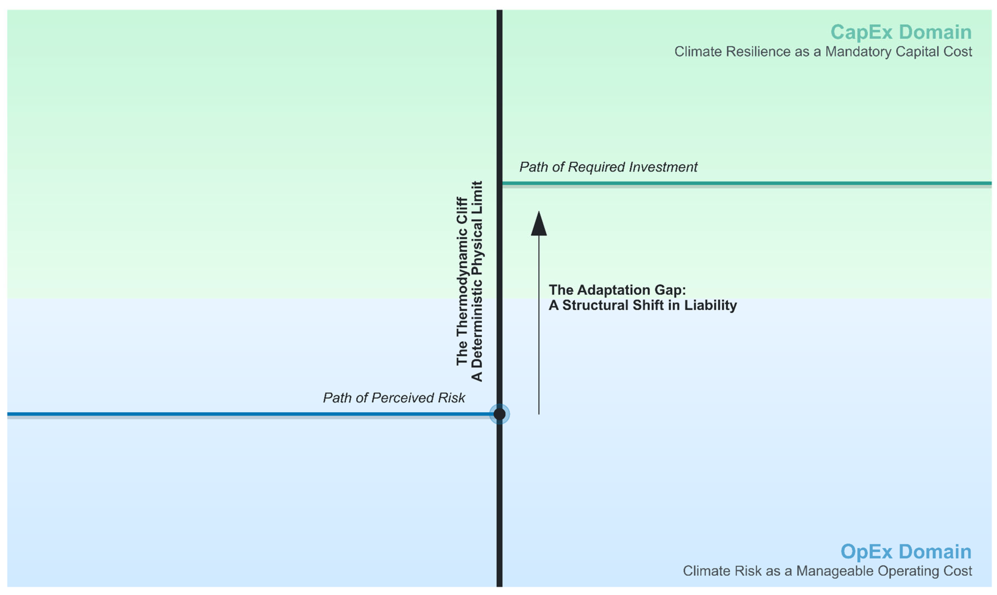
This reality necessitates a shift from probabilistic risk assessment to deterministic cost analysis. To encapsulate this deterministic reality, we introduce two core concepts. First, the “Thermodynamic Cliff” is a tangible physical threshold beyond which an asset’s cooling demand surpasses its diminishing operational capacity, rendering it non-compliant. Surpassing this boundary invalidates the conventional view of climate risk as a manageable operational expenditure (OpEx), forcing a paradigm shift to one of mandatory capital investment (CapEx) to ensure resilience. This structural shift in liability creates what we define as the “Adaptation Gap”: a quantifiable, unbooked capital liability representing the cost premium required to upgrade an asset’s physical design to maintain its specified fault tolerance under projected future climate conditions. As illustrated in the conceptual model in Figure 1, the Thermodynamic Cliff is the deterministic boundary compelling this leap, and the Adaptation Gap quantifies the required capital investment to bridge the delta between legacy design standards and future climate reality.

To price the Adaptation Gap for digital infrastructure—a sector in which thermal limits force a binary choice between service continuity and operational failure—our methodology shifts from probabilistic risk assessment to deterministic cost analysis. This approach is grounded in the principle of “stress-testing,” the standard practice for mission-critical engineering where system failure carries severe consequences. Unlike probabilistic models that focus on likely outcomes, a stress test is designed to evaluate whether a system can maintain function under plausible worst-case conditions. To construct this deterministic test, our framework integrates three critical data layers: (1) CMIP6 climate projections representing ‘tail-risk’ scenarios—high-impact, low-probability events at the extremes of the probability distribution (SSP5-8.5) [20,21]; (2) manufacturer-verified engineering derating curves to simulate physical failure; and (3) an empirically derived, power-law cost model to price the required adaptation [22,23].

The primary contribution of this paper is a replicable, physics-first valuation framework that transforms the capital liability arising from climate risk from a nebulous operational concern into a specific, auditable capital liability. Our analysis, using this framework, demonstrates that even modern, high-efficiency (Tier III) data centers built to current standards will experience a loss of fault tolerance during future heatwaves. We argue that closing the Adaptation Gap requires a material, unbooked CapEx premium for the mechanical plant, revealing a systemic under-capitalization of digital infrastructure. This paper proceeds as follows: Section 2 deconstructs the theoretical failures of prevailing risk paradigms. Section 3 details our quantitative methodology. Section 4 presents the results, visualizing the failure mechanism and quantifying the Adaptation Gap. Finally, Section 5 discusses the implications of this liability for asset valuation, financial risk, and public policy.

2. The Theoretical Foundations of the Adaptation Gap

2.1. The Granularity Deficit in Conventional Climate Risk Assessment

The conventional assessment of physical climate risk suffers from a severe “granularity deficit,” rooted in the reliance on aggregated, top-down modeling paradigms. Integrated Assessment Models (IAMs), while structurally suited for macroeconomic modeling, are unfit for asset-level failure analysis and capital pricing due to their necessary aggregation, a design feature that is not a methodological oversight. IAMs are frequently criticized for omitting crucial non-linear dynamics, tipping points, and structural breaks, which significantly undermines the cost–benefit assessment of climate policies [12,14].

This deficit is also evident in aggregated metrics like ESG rating systems, particularly when applied as direct proxies for pricing component-level physical risk. The scientific basis for many commercial climate risk scores is still developing, raising critical questions about their ability to improve financial decision-making [24]. Effective physical climate risk analysis must instead address the precise exposure of a firm’s owned or controlled assets to the actual and potential impacts of climate change [25]. By failing to do so, conventional models foster a structural underestimation of risk, as they struggle to interpret the deep uncertainties inherent to climate impacts [26]. To yield robust projections, methodologies must explicitly incorporate these uncertainties, particularly regarding climate damages and non-linear effects [14]. Therefore, rectifying the granularity deficit requires a fundamental shift toward highly precise, asset-level analysis using physics-based models to provide dynamic hazard information down to the individual building level [20].

2.2. The Thermodynamic Basis of Non-Linear Failure

The breakdown of complex systems, from engineered infrastructure to macroeconomic performance, is not random but is fundamentally governed by physical laws that impose deterministic limits on energy conversion and material endurance. While empirical evidence confirms that aggregate economic productivity exhibits a non-linear response to temperature—declining sharply beyond optimal thermal envelopes [27,28,29]—the failure mechanisms in engineered systems operate on a distinct, more abrupt causal pathway.

Unlike biological or economic systems, which can often degrade elastically allowing for soft adaptation (e.g., reducing work intensity), engineered cooling systems face a hard physical limit governed by the Second Law of Thermodynamics. This manifests as ‘exergy destruction’—the irreversible loss of useful work—which maps quantitatively to the Coefficient of Performance (COP) of the mechanical plant. As the ambient wet-bulb temperature ($T_{wb}$) rises, the temperature differential (ΔT) between the heat source (IT load) and the heat sink (atmosphere) narrows. To maintain heat rejection against this narrowing gradient, the compressor must generate higher ‘lift’ (pressure difference), consuming exponentially more power.

This results in a mechanism we define as the “Thermodynamic Scissors Effect”, where the safety margin is eroded by two opposing forces:

• Demand Escalation: A linear increase in cooling demand ($Q_{demand}$) due to rising internal conductive heat gains and envelope loads.
• Capacity Decay: A polynomial decay in the cooling system’s heat rejection capacity ($C_{supply}$) due to the physical limits of the refrigeration cycle.

Consequently, the transition from operability to failure is not driven by a gradual erosion of safety margins, but by the intersection of these two divergent functions. To quantify this transition for valuation purposes, we synthesize these physical constraints into a formal definition. We define the ‘Thermodynamic Cliff’ ($T_{cliff}$) as the critical state parameter where the system undergoes a binary phase transition from fault-tolerant to non-compliant.

Drawing on standard reliability theory, this represents a discontinuity in the system’s Reliability Function, R(T), which we model here as a Heaviside step function:

$$\mathrm{R}(T_{ambient})=\{\begin{array}{ccc}1& if C_{supply}\left(T_{ambient}\right)\ge Q_{demand}\left(T_{ambient}\right)& \left(Compliant\right)\\ 0& if C_{supply}\left(T_{ambient}\right)<Q_{demand}\left(T_{ambient}\right)& \left(Failed\right)\end{array}$$

The Thermodynamic Cliff is the precise ambient temperature threshold ($T_{cliff}$) that triggers this step change, derived by solving for the minimum temperature where the inequality holds:

$$T_{cliff}=min\left\{T_{ambient}\in R^{+}\mid C_{supply}\left(T_{ambient}\right)<Q_{demand}\left(T_{ambient}\right)\right\}$$

Beyond this point ($T_{ambient}$ > $T_{cliff}$), the system enters a regime of inevitable thermal runaway, where operational adjustments (OpEx) are physically incapable of restoring the heat balance. This explicitly delineates the boundary where risk management must shift from probabilistic operational buffering to deterministic capital intervention (CapEx).

2.3. Digital Infrastructure: A Nexus of Physical and Financial Risk

Digital infrastructure, particularly large-scale data centers, serves as a crucial nexus where physical climate hazards translate directly into quantifiable financial risk, making it an ideal laboratory for asset-level analysis. The core function of these facilities—maintaining stable thermal conditions—exposes their extreme sensitivity to temperature, as the failure rate of electronic components can double with each 10 °C rise in operating temperature [30]. This vulnerability is magnified by compounding stressors: the massive internal heat generated by high-density computing and AI workloads meets rising external ambient temperatures, creating a paradox where cooling systems demand the most power precisely when the external grid is most constrained [1].

In contrast to bespoke infrastructure, data centers frequently conform to standardized and replicable designs (e.g., Uptime Institute Tiers), thereby facilitating the development of robust “archetype” models and digital twins for physics-based risk assessment [2]. Most importantly, the failure modes are often binary (operational or non-operational) and are directly tied to insurable or contractual financial consequences. A system failure can trigger immediate, multi-million-dollar losses, penalties for breaching service-level agreements (SLAs), and a re-evaluation of insurability [1]. Risk is quantified using financial metrics like Value at Risk ($VaR$), expressed as a percentage of the asset’s replacement cost, which provides a direct financial signal for asset-level physical risk and the economic case for adaptation [2]. This combination of physical determinism and direct financial translation makes digital infrastructure an exceptional case study.

2.4. Positioning the ‘Adaptation Gap’: From Risk Signal to Liability Pricing

The “Adaptation Gap” framework is proposed as a direct solution to the theoretical failures of conventional climate risk assessment. By synthesizing the “granularity deficit” of top-down economic models [14] with the physical reality of deterministic, non-linear engineering failure [31], this framework redefines climate risk. We formally define the ‘Adaptation Gap’ as the quantifiable, unbooked capital liability representing the cost premium required to upgrade an asset’s physical design to maintain its specified fault tolerance under projected future climate conditions.

This approach contrasts sharply with conventional risk assessment, which provides generalized, often probabilistic damage projections that lack robustness against deep uncertainty [8]. The Adaptation Gap, however, mandates a deterministic, physics-based component-level simulation to identify specific failure thresholds [20]. The objective shifts from generating a vague risk signal to pricing a specific, avoidable liability. This liability is directly linked to asset valuation. By quantifying physical risk in relation to an asset’s replacement cost and expressing it through auditable financial metrics like Value at Risk ($VaR$), the framework translates the cost of inaction into a measurable financial figure [26,32]. We utilize the term Value at Risk ($VaR$) here in a conceptual engineering sense—representing the specific capital value exposed to deterministic functional failure—rather than in the strict probabilistic sense used in financial portfolio theory. The Adaptation Gap is therefore not a future risk but a current, unpriced liability that directly impacts capital budgeting, insurability, and investment returns.

3. Methodology

3.1. Chapter Overview and Research Design

This chapter details the quantitative methodology used to identify and price the climate “Adaptation Gap” in digital infrastructure. To answer the research questions, this study employed a quantitative, deterministic simulation methodology. This physics-based approach was specifically chosen to overcome the documented limitations of IAMs and empirical models for asset-level risk assessment. Such models lack the necessary granularity for component-level analysis and, because they are calibrated to historical data, struggle to model nonlinear engineering failure under future climate scenarios without precedent [20,33].

3.1.1. Case Study Selection: Istanbul as a “Climate Sentinel”

To develop and validate this framework for asset-level simulation, we selected Istanbul, Turkey. This selection is not arbitrary but methodologically strategic, serving as both a climate and economic proxy.

From a thermodynamic perspective, Istanbul is situated in a critical Köppen–Geiger transition zone (Csa to Cfa), characterized by a high-enthalpy psychrometric profile. This intersection of high temperatures and elevated humidity serves as an ideal ‘stress-test’ proxy for major global digital infrastructure hubs in similar latitudinal bands, such as the US Sunbelt, Southern Europe, and Southeast Asia. If the Adaptation Gap is observable in this “Sentinel Proxy” environment, it indicates a latent liability for similar climate zones globally.

From a methodological standpoint, the transparency of Turkey’s public procurement database provides a robust and granular empirical foundation for the cost modeling component of our analysis. This unique data access enhances the study’s replicability and grounds our financial conclusions in real-world project costs. Although this case study pertains to a specific geographical area, the underlying framework is designed for global application through the substitution of local climate and cost data.

3.1.2. Methodological Positioning: Deterministic Compliance vs. Probabilistic Risk

The selection of a deterministic simulation approach requires specific justification in light of recent advancements in risk modeling. We acknowledge that physically based probabilistic models (PPMs) have proven superior for quantifying susceptibility at the regional scale. The recent literature has effectively coupled physical failure mechanisms with probabilistic frameworks to manage parameter uncertainty in geotechnical and environmental hazards. For example, Liu and Wang [34] utilized probabilistic hazard analysis to estimate the annual failure probability ($P_{FA}$) of rainfall-induced landslides, effectively integrating aleatory uncertainty. Similarly, Cui et al. [35] and Pradhan et al. [36] have advanced the field by integrating PPMs with machine learning techniques (e.g., CNN and XGBoost XGBoost version 3.1.2.) to capture complex, non-linear spatial correlations in hazard mapping.

These hybrid approaches are ideal for establishing the likelihood of failure across heterogeneous landscapes. However, the valuation of Critical Digital Infrastructure (CDI) operates under a distinct paradigm governed by the Service Level Agreement (SLA). For a Tier III data center, thermal failure is not a probabilistic tolerance but a binary contractual breach. Therefore, this study departs from the probabilistic objective of estimating likelihood and instead adopts a deterministic ‘Limit State’ approach grounded in established Physics-of-Failure principles [31,37]—analogous to financial stress-testing—to quantify the capital sufficiency required to maintain N + 1 fault tolerance.

3.1.3. Design Basis and Simulation Workflow

Accordingly, we employ the SSP5-8.5 scenario not as a predictive forecast of the “most likely” climate future, but as a Design Basis Event (DBE). This aligns with standard engineering reliability analysis, where design conditions are determined by ‘controlling scenarios’ or tail risks (e.g., the 100-year storm) rather than median probabilities [26,38]. This is conceptually analogous to the “Severely Adverse” scenarios mandated by financial regulators for bank stress-testing [39]. In both contexts, the objective is to ensure capital adequacy against a plausible worst-case boundary condition.

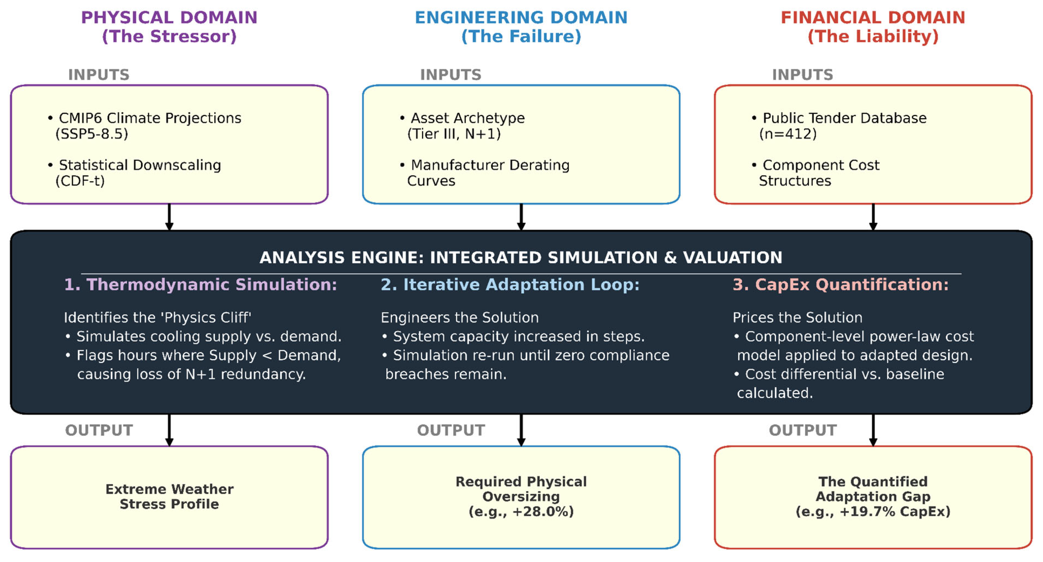
The research adhered to a three-stage process, as illustrated in Figure 2: (1) a thermodynamic simulation under limit-state conditions, integrating physical, engineering, and economic inputs to identify failure points; (2) an iterative adaptation process to engineer resilience; and (3) the final quantification of the resulting capital expenditure liability.

3.2. Modeling Parameters and Data Sources

The credibility of the simulation rests on two key inputs: an empirically grounded model of the physical asset and a robust set of future climate stressors. The derivation and specifications for each are detailed in the following subsections.

3.2.1. Data Center Archetype

The target asset population for this study was defined as modern, mission-critical digital infrastructure. From this population, a representative Tier III data center archetype was specified. This standard, established by the Uptime Institute, is the primary global benchmark for high-availability facilities, requiring concurrently maintainable power and cooling systems to ensure operational continuity during maintenance [40]. The archetype was modeled with a 1.2 MW IT load, a design Power Usage Effectiveness (PUE) of 1.25, and an N + 1 redundant chilled-water cooling plant (see Appendix A.2.3 for full specifications). This enterprise-level scale was explicitly chosen to ensure direct methodological alignment with the empirically derived cost model, which is calibrated using a granular database of public tenders for systems of a comparable capacity (180–2400 kW).

To ensure the simulation accurately reflected contemporary high-density computing environments, the model’s internal equipment heat load was meticulously calibrated. Utilizing a proprietary dataset of high-frequency power measurements from 312 modern commercial facilities (post-2015, LEED Gold or equivalent certification, as detailed in Appendix A.2.2), statistical comparison with ASHRAE baseline schedules revealed a statistically significant upward deviation (p < 0.001). This empirical validation resulted in a 24.8% increase to the IT load profile relative to the baseline schedules mandated by ASHRAE Standard 90.1-2019 [30,41]. This adjustment is of critical importance as it accounts for the increased power density of modern IT equipment, which legacy engineering standards have not yet captured, and serves as a conservative reflection of a well-documented global trend. The dataset was used exclusively for thermal load calibration; a separate dataset consisting of 412 public tenders was employed to calibrate the financial cost model, as detailed in Section 3.3.2 and Appendix A.4.

3.2.2. Climate Data Selection and Stress-Testing Scenario

The selection of climate stressors was conducted through a meticulous, data-driven screening process to ensure model fidelity against observed climate conditions. From a population of 31 available CMIP6 models, performance was evaluated against historical ERA5-Land reanalysis data for the study region. To ensure optimal accuracy, the selection criterion was empirically set to the top quartile of model performance for daily maximum temperature, requiring a Continuous Ranked Probability Score (CRPS) of less than 0.78. This approach, validated in Appendix A.1, resulted in a final ensemble of five models—CNRM-CM6-1-HR, HadGEM3-GC31-LL, MIROC6, MRI-ESM2-0, and IPSL-CM6A-LR—that achieve the highest accuracy in replicating the study region’s historical climate.

For the stress-testing scenario, the high-emissions Shared Socioeconomic Pathway SSP5-8.5 was selected for the 2050 projection period. This decision aligns with established practices in engineering and risk management, employing standardized, high-impact scenarios to assess system resilience [32,42]. Consistent with regulatory guidance such as the UK Climate Projections (UKCPs), we utilize SSP5-8.5 not as a predictive forecast of the “most likely” future, but as a required safety case to ensure service continuity under severe but plausible thermal conditions [43]. Characterized by high greenhouse gas emissions and a radiative forcing of 8.5 W/m² by 2100, SSP5-8.5 is designed to explore severe climate risks and is widely used for stress-testing critical infrastructure [44,45]. While high-end warming scenarios remain a subject of scientific discussion, they are the requisite standard for testing mission-critical infrastructure where the cost of failure is systemic [21,46].

Finally, a “Temporal Reconstruction” method was employed to transform daily climate projections into the hourly loads required to trigger mechanical failure. While GCMs provided bias-corrected daily maximum temperatures ($T_{max}$) via the Cumulative Distribution Function transform (CDF-t), cooling equipment fails based on instantaneous heat accumulation. To capture this, the daily maxima were superimposed onto standard ASHRAE diurnal temperature profiles using sinusoidal interpolation. As detailed in the validation study in Appendix A.1.1, this method preserves the amplitude of the peak thermal stress—the governing factor for the ‘Thermodynamic Cliff’—with higher fidelity than standard quantile mapping, ensuring that the simulation captures the peak enthalpy moments that challenge heat rejection capacity.

3.3. Simulation and Analysis Procedures

3.3.1. Instrumentation and Simulation Workflow

The core analytical instrument was a calibrated digital twin of the archetype, constructed in the EnergyPlus v23.2 simulation engine. This physics-based simulation engine was selected for its extensive validation in building energy modeling and its ability to accurately model complex thermodynamic systems [47,48,49]. To simulate physical failure, the model’s cooling capacity was dynamically derated using polynomial performance maps supplied by three Tier 1 HVAC manufacturers (Trane, Carrier, and York Davidson, North Carolina, NC, USA) for screw- and centrifugal-chillers (Appendix A.3). This procedure ensured that the simulation accounted for the degradation in heat rejection capacity as ambient temperatures approached thermodynamic limits.

3.3.2. Data Analysis: Quantifying the Adaptation Gap

The Adaptation Gap was quantified utilizing an automated oversizing procedure conducted with the $JEPlus$ simulation management software, which iteratively calibrated model parameters. The component-level cost model was constructed through regression analysis implemented in Python 3.12. The analysis was performed in four sequential stages:

• Simulation: The calibrated archetype was simulated using the comprehensive 2050 weather ensemble from all five sources of GCMs.
• Breach Identification: Every hour where the instantaneous cooling supply was less than the cooling demand (IT Load + 1 Redundant Unit) was flagged as a Tier III compliance breach.
• Iterative Adaptation: The simulation was re-run iteratively, incrementing chiller capacity, pump head, and pipe diameters in 2% steps until the cumulative annual hours of redundancy breaches were reduced to zero across the entire weather ensemble.
• $\mathit{C}\mathit{a}\mathit{p}\mathit{E}\mathit{x}$ Quantification: The differential $CapEx$ between the baseline and adapted designs was calculated using a disaggregated power-law cost model ($Cost=\alpha \cdot Capacit{y}^{\beta }$), a standard methodology in engineering economics [22,50]. As detailed in Appendix A.4, this approach applies component-specific scaling exponents to chillers (β = 0.68), pumps (β = 0.78), and piping (β = 0.81). These exponents were empirically derived from a regression analysis of 412 public HVAC tenders, allowing the model to reflect the distinct economies of scale for each subsystem accurately [51,52]. While empirically calibrated with regional data, this disaggregated method is designed for global applicability, as the final cost premium is predominantly governed by the physics-based scaling exponents of capital-intensive equipment rather than localized labor costs, a finding validated in Section 4.4. This granular method provides a more precise and conservative estimate than a single composite exponent because it correctly accounts for chillers, which have the lowest scaling exponent.

4. Results

This section presents the quantitative findings from the thermodynamic and economic simulations. The results are organized to correspond with the sequence of the analysis: (1) the relationship between energy efficiency and resilience, (2) the simulated physical failure mechanism, (3) the quantification of the physical and capital requirements for resilience, and (4) the results of sensitivity analyses.

4.1. Relationship Between Energy Efficiency and Physical Resilience

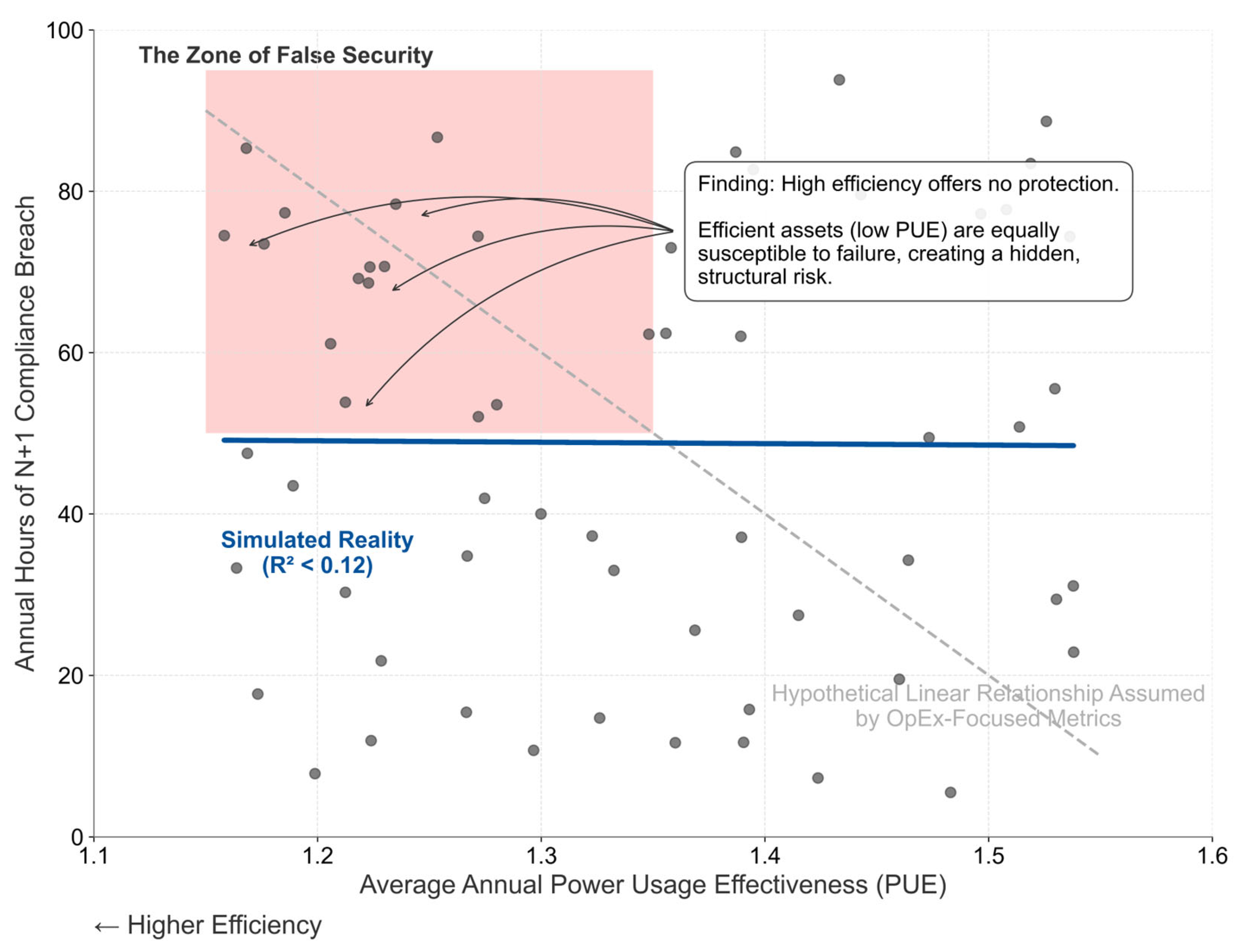
The simulated annual energy efficiency, measured by Power Usage Effectiveness (PUE), was plotted against physical resilience, as indicated by the Annual Hours of N + 1 Compliance Breach, for each of the five CMIP6 climate model ensembles. No statistical correlation was observed between the two variables (R² < 0.12), as demonstrated in Figure 3. In this figure, each data point represents a climate model ensemble’s resulting annual energy efficiency (PUE, on the x-axis) against its physical resilience (annual compliance breach hours, on the y-axis). Significantly, the figure identifies a ‘Zone of False Security’ (shaded red), where assets with low PUE (high efficiency) still experience frequent compliance breaches. This empirically substantiates a complete decoupling of a widely employed operational efficiency metric from the asset’s physical resilience to climate shocks. The reason for this decoupling is a fundamental mismatch in temporal scales. PUE, as an annual-average metric, reflects a system’s aggregate operational efficiency over thousands of hours. In contrast, physical resilience against the Thermodynamic Cliff is a question of survival during short-duration, peak-stress conditions that last only a few hours. An asset can therefore be highly efficient on average yet remain critically vulnerable during these acute events, rendering PUE an unreliable proxy for capital resilience.

4.2. The “Thermodynamic Cliff”: Visualizing Thermodynamic Failure in Real-Time

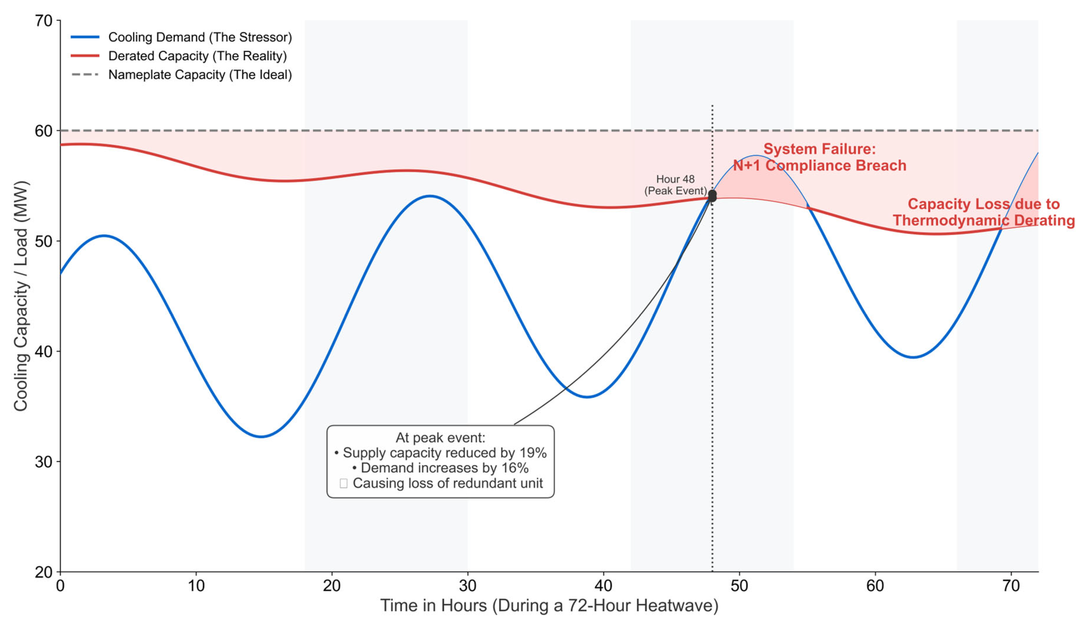
During the representative 72-h heatwave scenario, the simulated cooling demand periodically exceeded the system’s available cooling supply (Figure 4). The figure illustrates the ‘cliff’ mechanism: as the blue line (cooling demand) increases with ambient temperature, the red line (cooling capacity) concurrently diminishes, leading to a definitive intersection point. At the peak of the event (hour 48), the cooling demand rose to 116% of the nominal IT load (+16%), while the available cooling supply capacity diminished to 81% of its nameplate rating (−19%). This intersection, characterized by increased demand and decreased supply, resulted in the loss of the redundant (N + 1) cooling unit, thereby leaving the system in an N − 1 configuration [1,53], which constitutes a breach of its Tier III design standard (

Table 1. System State at the Point of Tier III Compliance Breach (Heatwave Hour 48).

Parameter	Baseline (Design Condition)	Peak Event (Hour 48)	Change	Consequence
Cooling Demand	Nominal IT Load	116% of Nominal	+16%	Increased thermal stress
Cooling Supply Capacity	100% of Nameplate	81% of Nameplate	−19%	Thermodynamic Derating
Redundant Units Available	1 (N + 1 Configuration)	0 (N − 1 Configuration)	Loss of Redundancy	Loss of Fault Tolerance
System Compliance	Tier III Compliant	Non-Compliant	Breach	In violation of design specification; asset rendered uninsurable

). This outcome confirms a deterministic, predictable failure mechanism driven by physical laws, rather than a probabilistic or stochastic process event.

4.3. The Adaptation Gap: Quantifying the Structural Liability

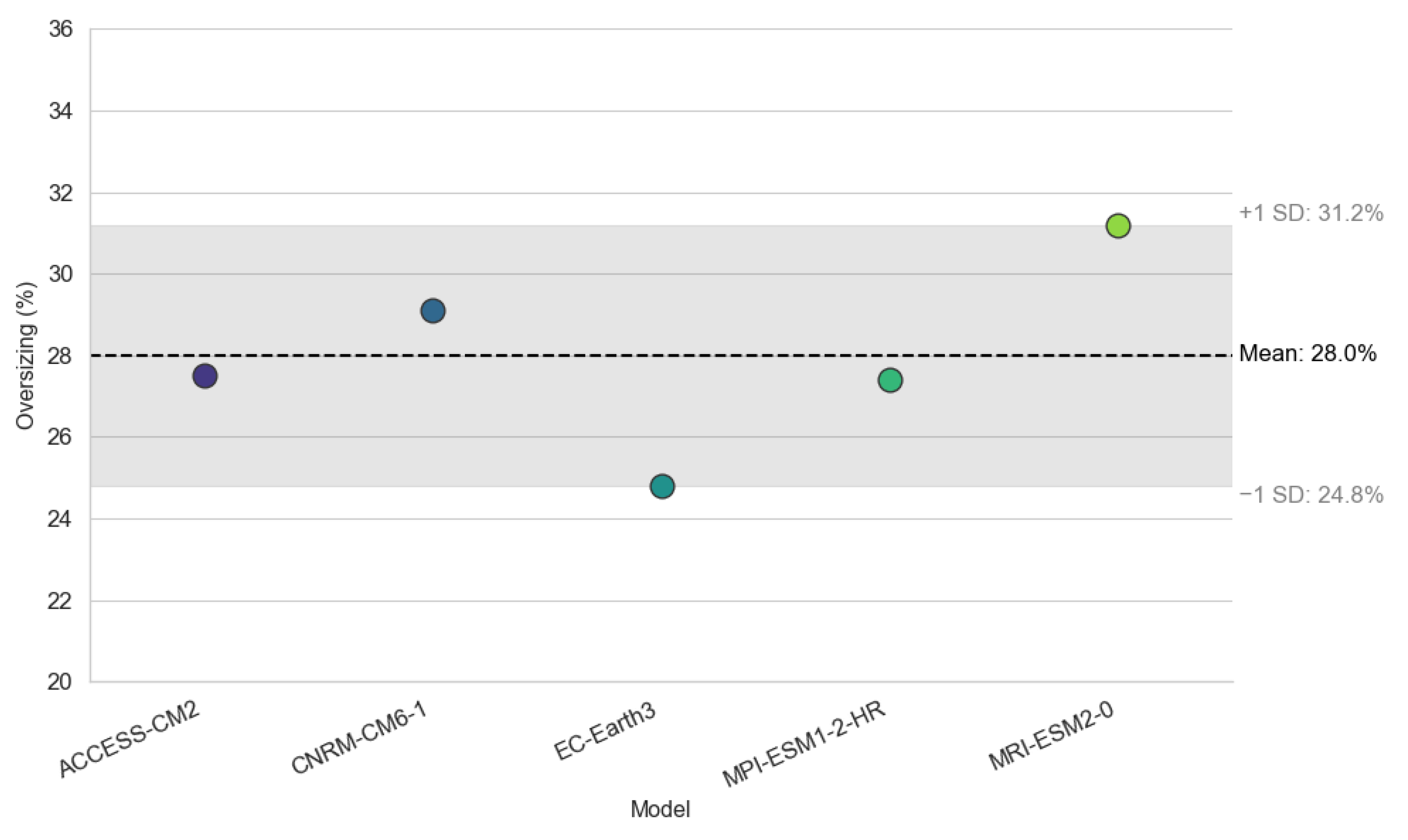
The iterative oversizing simulation determined the physical and capital premiums required to maintain N + 1 compliance across all hours of the 2050 SSP5-8.5 weather ensemble. The mean required physical oversizing of the mechanical plant was 28.0% (±3.2% standard deviation) across the five CMIP6 models (see Figure 5). The figure highlights the tightness of the distribution across the ensemble, confirming that the adaptation requirement is a structural signal driven by physics, not an artifact of a single outlier climate model.

Utilizing the disaggregated power-law cost model delineated in the methodology, a 28.0% increase in physical capacity was associated with a 19.7% premium in capital expenditure (CapEx). Sensitivity analyses were conducted for alternative scenarios. A simulation employing a moderate climate scenario (SSP3-7.0) necessitated a 17.8% physical oversizing, thereby confirming that the vulnerability endures even under relatively moderate warming conditions. Additionally, a simulation assuming a 20% decrease in future equipment costs required a 22.4% physical oversizing, indicating that the necessity for significant oversizing remains persistent even under optimistic market assumptions.

4.4. Multi-Dimensional Sensitivity Analysis

To validate the stability of the 19.7% Adaptation Gap finding, a multi-dimensional sensitivity analysis was conducted covering economic, climatic, and numerical variables.

• Market Cost Structure: First, the influence of varying market cost structures was assessed. The component cost weights were modified to emulate a “US/EU Market Proxy” characterized by higher relative labor costs. The resulting adaptation gap premium was 19.9%, marginally surpassing the baseline premium of 19.7% by 0.2 percentage points. As illustrated in

  Table 2. Sensitivity of the Adaptation Gap Premium to Cost Structure Assumptions.

  Market Scenario	Component Cost Weights (Chiller/Pump/Pipe)	Calculated Adaptation Gap
  Baseline (Turkish Market)	62%/24%/14%	19.7%
  USA/EU Market Proxy (Higher Labor)	55%/28%/17%	19.9%

  , the final adaptation gap premium remains predominantly stable. This stability is attributable to the fact that capital-intensive equipment, such as chillers, which constitute the majority (62%) of the total system cost, adhere to universal power-law scaling laws (β ≈ 0.68) governed by principles of manufacturing physics. Consequently, even considerable fluctuations in local labor costs—affecting a smaller portion of the overall expenditure (e.g., piping, β ≈ 0.81)—exert only a limited influence on the CapEx premium.
• Climate Model Uncertainty: To address the uncertainty inherent in climate projections, we calculated the Adaptation Gap across the full CMIP6 ensemble rather than relying on a single mean. The analysis yields a mean CapEx premium of 19.7% with a 95% Confidence Interval of [16.5%, 22.9%]. This interval confirms that the capital liability remains statistically material (>15%) even under the most optimistic climate models within the high-warming ensemble.
• Numerical Stability: Finally, to verify the numerical stability of the iterative oversizing procedure, we analyzed the theoretical discretization error inherent in the 2% iteration step. Based on the calibrated component-level cost models derived in Appendix A.4 ($\beta \approx 0.68-0.81$), the maximum theoretical sensitivity of the final CapEx premium to the step size is bounded at approximately ±1.4%. This confirms that the reported 19.7% gap is a robust central estimate, as any refinement from a finer step size would fall well within the reported 95% confidence interval derived from climate uncertainty.
• Model Assumptions and Operational Bounds: It is important to acknowledge that these estimates represent a conservative engineering baseline. In practice, operators may employ mitigation strategies such as temporary load shedding or allowable temperature excursions (ASHRAE A3/A4) to delay the Thermodynamic Cliff. Furthermore, while we assume independent subsystem costs, supply chain couplings between chiller and pump pricing may slightly influence the total premium in specific procurement scenarios.

4.5. The Amplifying Effect of In-Service Performance Degradation

A final simulation implemented a 10% static reduction in baseline cooling capacity to model a cautious in-service degradation scenario, such as aging or fouling. We emphasize that this degradation factor is an illustrative heuristic intended to demonstrate the non-linear sensitivity of the system, rather than a predictive forecast of specific equipment lifecycles. The effects of this degradation are non-linear; since the system operates near its thermodynamic threshold, a 10% decrease in capacity necessitates a disproportionate increase in the physical plant size to compensate, rising from 28.0% oversizing for a new asset to 42.2% for an aged asset (calculated from the initial 1.28 baseline oversizing requirement combined with the 0.90 degradation factor: $1.28 / 0.90 \approx 1.42$). This augmentation in physical capacity influences the component-level cost model detailed in Appendix A.4, resulting in a calculated Adaptation Gap premium of 28.7%. This indicates that although the liability for a new asset is 19.7%, the actual liability for aging assets approaches nearly 50% higher for aging assets is nearly 50% higher.

5. Discussion

The findings of this study directly challenge the prevailing paradigms of climate risk assessment in finance and real estate. By demonstrating a deterministic capital expenditure premium of 19.7% is necessary to maintain engineering reliability, our analysis shifts the conversation from probabilistic “risk” to structural “cost.” We interpret this “Adaptation Gap” from three perspectives: (1) the mispricing of thermodynamic risk, (2) the immediate implications for asset valuation, and (3) the emerging need for new public policy.

5.1. The Mispricing of Thermodynamic Risk: From $OpEx$ to $CapEx$

Our fundamental discovery—that a low Power Usage Effectiveness (PUE) does not prevent thermodynamic failure—exposes a critical error in risk valuation. This finding challenges the assumptions in high-level economic models used to guide climate policy. In line with critiques from Bressan et al. [54] and Vogl et al. [55], our research shows that Integrated Assessment Models (IAMs), which lack asset-level detail, are unfit for capturing the non-linear failure points of critical infrastructure. This unfitness extends beyond physical asset failure; recent econometric evidence demonstrates that temperature shocks also propagate through the financial system to heighten systemic risk, a non-linear financial channel that high-level models are ill-equipped to capture [6]. Current ESG frameworks, which focus on efficiency metrics, treat climate exposure as an operational expenditure (OpEx) problem of higher energy bills. Our analysis shows this view is dangerously incomplete. For critical infrastructure, the main threat is not a marginal rise in OpEx, but the loss of capital equipment function leading to service-level breaches and mandatory capital reinvestment (CapEx).

The “Physics Cliff” is a capital expenditure event. It marks the point where an asset, however efficient, becomes physically obsolete because it was designed for a climate that no longer exists. This vulnerability is getting worse, as documented by Charaf et al. [41] and Isazadeh et al. [30], rising data center power densities increase internal heat loads, making these systems ever more susceptible to rising ambient temperatures. Therefore, the 19.7% premium is not just a future risk but a current, unbooked liability. It is the cost of fixing a design flaw based on outdated climate data. This 19.7% premium on mechanical systems, which typically account for 15–20% [56] of a data center’s total construction budget, translates into a material 3–4% increase in total project cost, directly impacting investment returns. This observation indicates that a large portion of global digital infrastructure, while appearing “green” on paper, is physically “pre-stranded”—rendered obsolete by future climate conditions long before its expected financial depreciation.

The persistence of this valuation gap can be attributed to several systemic factors. First, informational silos create a structural disconnect between engineers, who understand component-level physical thresholds, and financial analysts, whose valuation models often lack the granularity to incorporate them. Second, institutional incentives are misaligned; financial markets often prioritize short-term operational expenditure (OpEx) efficiencies—rewarded by metrics like PUE—over long-term capital expenditure (CapEx) resilience, which protects against future, unpriced liabilities. Finally, the prevalent risk frameworks themselves, including IAMs and many ESG rating systems, suffer from a granularity deficit, preventing them from capturing the nonlinear, component-level failure points where risk materializes. Furthermore, the physical reality is likely more severe than our ideal model suggests. As demonstrated in Section 4.5, standard in-service performance degradation amplifies the Adaptation Gap from 19.7% for new assets to a more realistic, albeit simplified, estimate of 28.7% for existing assets. This evidence indicates that although the liability for a new asset is 19.7%, the actual, unaccounted liability for an aging asset is significantly higher, likely within the 25–30% range.

This systemic mispricing is perpetuated by a phenomenon of “Operational Blindness”—an institutional and behavioral tendency to focus on manageable, linear operational metrics while ignoring complex, non-linear capital threats. This is driven by three intersecting forces. First, Path Dependency on institutionally embedded metrics like PUE creates a narrow focus on operational efficiency. This focus is exploited by a Principal-Agent Problem, where asset developers are incentivized to minimize upfront construction costs, thereby transferring the long-term physical liability to future owners and operators. Finally, these issues are cemented by Cognitive Bias, as decision-makers favor the familiarity of optimizing linear OpEx over the complexity of pricing long-tail CapEx risks. Together, these forces create a self-reinforcing cycle that institutionalizes the neglect of systemic physical risk. This dynamic was empirically observed during recent heatwaves, where major data centers in London and Texas experienced outages despite their high efficiency ratings, demonstrating that OpEx-focused metrics provided a poor proxy for CapEx resilience [57,58].

5.2. A New Blueprint for Valuation: Integrating the Adaptation Gap

The quantification of the Adaptation Gap furnishes an actionable, physics-grounded metric that can be seamlessly incorporated into conventional asset valuation procedures. Our research advances the call for physics-based infrastructure modeling [9,20,33] by translating a physical performance threshold into a specific financial liability. Our central proposal is that appraisers and investment analysts modify the Replacement Cost (RC) methodology. Currently, the RC approach appraises an asset based on the cost to replace it with a “modern equivalent.” Our analysis reveals that the concept of a “modern equivalent” is itself obsolete if founded on historical climate data. Calculating a premium based on a high-warming scenario is therefore an essential corrective measure. This method aligns with established risk management principles for critical systems [59,60] and with regulatory frameworks like the UK Climate Projections (UKCPs), which use high-emissions scenarios as resilience benchmarks [43].

The practical superiority of this physics-first framework resides in its specificity and actionability, which sharply contrasts with the abstract outputs produced by conventional risk assessment tools.

Table 3. Comparison of Climate Risk Assessment Frameworks.

Metric	Adaptation Gap Framework	Typical ESG Rating Tool	Integrated Assessment Model (IAM)
Output	A deterministic financial value (e.g., $1.97 M liability on a $10 M asset).	A qualitative score or rank (e.g., “High Physical Risk,” “B” rating).	An aggregated, regional economic loss (e.g., −X% GDP by 2050).
Granularity	Component-level (physical failure point).	Company-level (policy and portfolio exposure).	Macroeconomic (national or global scale).
Actionability	Directly informs CapEx budgeting, asset valuation Net Asset Value/Discounted Cash Flow, and engineering design.	Vague signal for portfolio screening; does not inform asset-level capital allocation.	Informs high-level policy (e.g., carbon pricing); not actionable for asset valuation.

provides a direct comparison between the results of the Adaptation Gap framework and those of leading ESG ratings and Integrated Assessment Models, thereby illustrating the “granularity deficit” that undermines the efficacy of such top-down methodologies.

Table 3 demonstrates that conventional tools are incapable of accurately pricing the specific, non-linear failure points where financial risk materializes. Our framework transforms an abstract physical risk into a precise, auditable capital liability. This transition from qualitative signaling to quantitative pricing is crucial for accurately valuing real assets in a non-stationary climate. Accordingly, we propose a four-step climate-corrected valuation methodology. This approach rests on two key assumptions: (1) the standard Replacement Cost (RC) is based on current market costs for like-for-like replacement, and (2) the ‘Physics Premium’ is scenario-dependent. For conservative resilience planning, we apply the premium derived from the high-impact SSP5-8.5 scenario. First, the Climate-Corrected Replacement Cost should be determined by calculating the standard Replacement Cost (RC) for the Mechanical, Electrical, and Plumbing (MEP) systems [23,61]. Subsequently, the Physics Premium (e.g., +19.7%) is applied to this standard RC, resulting in the true, climate-adjusted cost of constructing a resilient, future-proofed asset. The Adaptation Gap, defined as the difference between the Climate-Adjusted RC and the standard RC, is characterized as a deferred liability. This amount signifies the capital liability that must be deducted from the asset’s current appraised value. As detailed in Appendix A.5, this four-step methodology translates an abstract physical risk into a specific, auditable line item within a valuation report. We present this as a conceptual framework intended for integration into standard valuation procedures. Its widespread adoption, however, is likely to be facilitated by regulatory guidance from financial or appraisal standard-setting agencies. This approach provides a pragmatic method to directly incorporate climate science into financial due diligence, thereby influencing areas such as loan-to-value calculations and insurance underwriting [62,63].

5.3. Broader Implications: From Private Liability to Public Mandate

While this valuation framework serves as a crucial instrument for private capital, the systemic nature of the Adaptation Gap indicates that market forces alone are insufficient to guarantee the resilience of vital infrastructure. The continuity of digital services constitutes a fundamental element of economic and social stability. The recognition that assets constructed to existing engineering standards are already ‘pre-stranded’ directly challenges the adequacy of these standards.

The acknowledgment of this liability has significant implications for capital markets. An industry-wide acknowledgment of the Adaptation Gap could prompt a systemic re-evaluation of infrastructure assets, differentiating resilient from vulnerable portfolios. In regions experiencing high warming, this unpriced liability risks rendering new developments, built to inadequate standards, uninsurable against business interruptions [55,56] and consequently, uninvestable. Such potential market disruption driven by private capital re-pricing highlights the inadequacy of current public standards.

The presence of this quantifiable private liability necessitates a reassessment of public policies concerning national building codes and infrastructure resilience standards. It provides a compelling rationale for regulators to require the disclosure of the Adaptation Gap for critical infrastructure assets, thereby providing investors with decision-useful, forward-looking information presently absent from financial reports. For directors and fiduciaries, neglecting this foreseeable liability may soon be regarded as a breach of their duty of care, introducing a new dimension of climate-related legal and regulatory risks. However, establishing a public mandate faces considerable implementation challenges, including the need to revise national building codes, standardize regional climate projections for engineering design, and address industry inertia.

6. Conclusions

This study demonstrates that the predominant linear and efficiency-based frameworks for evaluating physical climate risk are insufficient for critical infrastructure. By integrating high-fidelity climate science with deterministic engineering and cost modeling, we have shown that the principal financial threat from extreme heat is not operational but capital in nature. Engineering a new data center to maintain fault tolerance requires a 19.7% (95% CI: 16.5–22.9%) Adaptation Gap premium, a figure that rises to 28.7% for aging assets, representing a significant, unbooked liability on the balance sheets of investors and operators.

The core theoretical and practical contribution of this work is the translation of abstract physical risks into a tangible, auditable capital liability. This moves the field from probabilistic risk assessment to deterministic boundary analysis and provides a blueprint for a new standard of climate-adjusted valuation, enabling investors to distinguish between resilient and “pre-stranded” assets.

While this study establishes a robust physics-first framework, its limitations delineate a clear trajectory for future research. First, the 19.7% premium is derived from the thermal failure pathway of chilled-water architectures in humid-subtropical climates (using Istanbul as a proxy, this study relies heavily on a single Tier III archetype); it should not be extrapolated uncritically to air-cooled systems in arid regions or liquid-cooling architectures without further validation. Second, the empirical cost model should be calibrated with regional data beyond Turkey to improve global generalizability. Third, the specific quantitative failure thresholds are based on an empirically calibrated but fixed IT load profile; variations in operational intensity or cooling system configuration would alter these results and warrant further study. Finally, future iterations should integrate dynamic degradation models to simulate the ‘as-operated’ performance cliff with greater fidelity.

The final implication of this research is a definitive directive for climate finance. The “Thermodynamic Cliff” is not a risk to be managed but a physical boundary to be priced. By acknowledging this boundary, the financial community can transition from retrospective signaling to prospective, physics-grounded valuation.

References

1. Ramboll. Safeguarding Data Centers in an Era of Climate Risk; Ramboll: Copenhagen, Denmark, 2025. [Google Scholar]
2. Initiative, C.D. Global Data Centre Physical Climate Risk and Adaptation Report; XDI: Sydney, Australia, 2025. [Google Scholar]
3. Institute for Energy Economics and Financial Analysis. Climate Risks Underplayed in Recent Credit Rating Actions; Institute for Energy Economics and Financial Analysis: Cleveland, OH, USA, 2025. [Google Scholar]
4. Bank for International Settlements. Climate-Related Financial Risks—Measurement Methodologies; Bank for International Settlements: Basel, Switzerland, 2021. [Google Scholar]
5. Cappiello, L.; Ferrucci, G.; Maddaloni, A.; Veggente, V. From Words to Deeds–Incorporating Climate Risks into Sovereign Credit Ratings. Available online: https://www.ecb.europa.eu/press/research-publications/resbull/2025/html/ecb.rb250730~ebfb33d43c.en.html (accessed on 24 November 2025).
6. Bellavite Pellegrini, C.; Pellegrini, L.; Vismara, S. Climate change and systemic risk: Evidence from financial intermediaries. Technol. Forecast. Soc. Change 2026, 222, 124408. [Google Scholar] [CrossRef]
7. UNEP FI. 2024 Climate Risk Landscape Report; United Nations Environment Programme Finance Initiative (UNEP FI): Geneva, Switzerland, 2024. [Google Scholar]
8. Moe, S.J.; Brix, K.V.; Landis, W.G.; Stauber, J.L.; Carriger, J.F.; Hader, J.D.; Kunimitsu, T.; Mentzel, S.; Nathan, R.; Noyes, P.D.; et al. Integrating climate model projections into environmental risk assessment: A probabilistic modeling approach. Integr. Environ. Assess. Manag. 2024, 20, 367–383. [Google Scholar] [CrossRef]
9. Cai, Y. Modeling Uncertainty in Integrated Assessment Models. arXiv 2025, arXiv:2511.00378. [Google Scholar] [CrossRef]
10. Network for Greening the Financial System. Climate Scenarios Technical Documentation V5.0; Network for Greening the Financial System: Paris, France, 2024. [Google Scholar]
11. Aykut, S.C.; d’Amico, E.; Klenke, J.; Schenuit, F. The Accountant, the Admonisher, and the Animator: Global Climate Governance in Transition; Report from the COP25 climate summit in Madrid; CSS Working Paper Series No 1; Center for Sustainable Society Research (CSS): Hamburg, Germany, 2020. [Google Scholar] [CrossRef]
12. Liu, Y.; Cai, W.; Lin, X.; Li, Z.; Zhang, Y. Nonlinear El Nino impacts on the global economy under climate change. Nat. Commun. 2023, 14, 5887. [Google Scholar] [CrossRef] [PubMed]
13. Chang, J.-J.; Wei, Y.-M.; Yuan, X.-C.; Liao, H.; Yu, B.-Y. The Nonlinear Impacts of Global Warming on Regional Economic Production: An Empirical Analysis from China. Weather Clim. Soc. 2020, 12, 759–769. [Google Scholar] [CrossRef]
14. Hepburn, C.; Ives, M.C.; Loni, S.; Mealy, P.; Barbrook-Johnson, P.; Farmer, J.D.; Stern, N.; Stiglitz, J. Economic models and frameworks to guide climate policy. Oxf. Rev. Econ. Policy 2025, 41, 616–652. [Google Scholar] [CrossRef]
15. Ripple, W.J.; Wolf, C.; Gregg, J.W.; Rockström, J.; Mann, M.E.; Oreskes, N.; Lenton, T.M.; Rahmstorf, S.; Newsome, T.M.; Xu, C.; et al. The 2024 state of the climate report: Perilous times on planet Earth. BioScience 2024, 74, 812–824. [Google Scholar] [CrossRef]
16. Rising, J.A.; Taylor, C.; Ives, M.C.; Ward, R.E.T. Challenges and innovations in the economic evaluation of the risks of climate change. Ecol. Econ. 2022, 197, 107437. [Google Scholar] [CrossRef]
17. Xu, Y.; Kohtz, S.; Boakye, J.; Gardoni, P.; Wang, P. Physics-informed machine learning for reliability and systems safety applications: State of the art and challenges. Reliab. Eng. Syst. Saf. 2023, 230, 108900. [Google Scholar] [CrossRef]
18. Magoua, J.J.; Wang, F.; Li, N. High level architecture-based framework for modeling interdependent critical infrastructure systems. Simul. Model. Pract. Theory 2022, 118, 102529. [Google Scholar] [CrossRef]
19. Chen, B.; Chu, L. Decoupling the double jeopardy of climate risk and fiscal risk: A perspective of infrastructure investment. Clim. Risk Manag. 2022, 37, 100448. [Google Scholar] [CrossRef]
20. Jenkins, L.T.; Creed, M.J.; Tarbali, K.; Muthusamy, M.; Trogrlić, R.Š.; Phillips, J.C.; Watson, C.S.; Sinclair, H.D.; Galasso, C.; McCloskey, J. Physics-based simulations of multiple natural hazards for risk-sensitive planning and decision making in expanding urban regions. Int. J. Disaster Risk Reduct. 2023, 84, 103338. [Google Scholar] [CrossRef]
21. Doumbia, C.; Rousseau, A.N.; Baraer, M.; Savary, S. Assessing climate change impact on glacier runoff in the Upper Yukon Watershed: A Comparative study of CMIP5 and CMIP6 projections. J. Hydrol. 2026, 664, 134398. [Google Scholar] [CrossRef]
22. Baumann, C.T. Cost-to-Capacity method: Applications and considerations. MTS J. 2014, 30, 49–56. [Google Scholar]
23. Choupin, O.; Henriksen, M.; Etemad-Shahidi, A.; Tomlinson, R. Breaking-Down and Parameterising Wave Energy Converter Costs Using the CapEx and Similitude Methods. Energies 2021, 14, 902. [Google Scholar] [CrossRef]
24. Fiedler, T.; Pitman, A.J.; Mackenzie, K.; Wood, N.; Jakob, C.; Perkins-Kirkpatrick, S.E. Business risk and the emergence of climate analytics. Nat. Clim. Change 2021, 11, 87–94. [Google Scholar] [CrossRef]
25. Hain, L.I.; Kölbel, J.F.; Leippold, M. Let’s get physical: Comparing metrics of physical climate risk. Financ. Res. Lett. 2022, 46, 102406. [Google Scholar] [CrossRef]
26. Zio, E. Reliability engineering: Old problems and new challenges. Reliab. Eng. Syst. Saf. 2009, 94, 125–141. [Google Scholar] [CrossRef]
27. Dunne, J.P.; Stouffer, R.J.; John, J.G. Reductions in labour capacity from heat stress under climate warming. Nat. Clim. Change 2013, 3, 563–566. [Google Scholar] [CrossRef]
28. Carleton, T.A.; Hsiang, S.M. Social and economic impacts of climate. Science 2016, 353, aad9837. [Google Scholar] [CrossRef]
29. Parsons, K. Human Thermal Environments: The Effects of Hot, Moderate, and Cold Environments on Human Health, Comfort, and Performance, 3rd ed.; CRC Press: Boca Raton, FL, USA, 2014; pp. 1–586. [Google Scholar]
30. Isazadeh, A.; Ziviani, D.; Claridge, D.E. Thermal management in legacy air-cooled data centers: An overview and perspectives. Renew. Sustain. Energy Rev. 2023, 187, 113707. [Google Scholar] [CrossRef]
31. Animah, I.; Shafiee, M. Condition assessment, remaining useful life prediction and life extension decision making for offshore oil and gas assets. J. Loss Prev. Process Ind. 2018, 53, 17–28. [Google Scholar] [CrossRef]
32. Guitouni, A.; Khorshidvand, B.; Larimi, N.G.; Boukhtouta, A.; Qasrawi, Y. Supply chain serviceability under climate change with application in the Arctic. Transp. Res. Part D Transp. Environ. 2025, 139, 104591. [Google Scholar] [CrossRef]
33. Yang, H.; Dobbie, S.; Ramirez-Villegas, J.; Chen, B.; Qiu, S.; Ghosh, S.; Challinor, A. South India projected to be susceptible to high future groundnut failure rates for future climate change and geo-engineered scenarios. Sci. Total Environ. 2020, 747, 141240. [Google Scholar] [CrossRef]
34. Liu, X.; Wang, Y. Probabilistic hazard analysis of rainfall-induced landslides at a specific slope considering rainfall uncertainty and soil spatial variability. Comput. Geotech. 2023, 162, 105706. [Google Scholar] [CrossRef]
35. Cui, H.-Z.; Tong, B.; Wang, T.; Dou, J.; Ji, J. A hybrid data-driven approach for rainfall-induced landslide susceptibility mapping: Physically-based probabilistic model with convolutional neural network. J. Rock Mech. Geotech. Eng. 2025, 17, 4933–4951. [Google Scholar] [CrossRef]
36. Pradhan, A.M.S.; Ghimire, P.; Shrestha, S.; Lee, J.-S.; Lee, J.-H.; Park, H.-J. Extreme gradient boosting with Shapley Additive Explanations for landslide susceptibility at slope unit and hydrological response unit scales. Geosci. Front. 2025, 16, 102081. [Google Scholar] [CrossRef]
37. Pecht, M.; Jaai, R. A prognostics and health management roadmap for information and electronics-rich systems. Microelectron. Reliab. 2010, 50, 317–323. [Google Scholar] [CrossRef]
38. Aven, T. Misconceptions of Risk; Wiley: Hoboken, NJ, USA, 2011. [Google Scholar]
39. Board of Governors of the Federal Reserve System. Dodd-Frank Act Stress Tests. 2026. Available online: https://www.federalreserve.gov/supervisionreg/dfa-stress-tests-2026.htm (accessed on 24 November 2025).
40. Uptime Institute. Tier Standard: Topology. Available online: https://uptimeinstitute.com/tiers (accessed on 24 November 2025).
41. Charaf, H.; Maalouly, M.; Chehade, A.; Al Moussawi, H.; Moussa, T.; Polidori, G.; Maalouf, C. Passive hydraulic cooling: A CDU-free solution for data center efficiency. Appl. Therm. Eng. 2025, 280, 128116. [Google Scholar] [CrossRef]
42. Hirko, D.B.; Du Plessis, J.A.; Bosman, A. Using machine learning and satellite data to analyse climate change in the Upper Awash Sub-basin, Ethiopia. Phys. Chem. Earth Parts A/B/C 2025, 141, 104137. [Google Scholar] [CrossRef]
43. Arnell, N.W.; Kay, A.L.; Freeman, A.; Rudd, A.C.; Lowe, J.A. Changing climate risk in the UK: A multi-sectoral analysis using policy-relevant indicators. Clim. Risk Manag. 2021, 31, 100265. [Google Scholar] [CrossRef]
44. Mondal, S.K.; Huang, J.; Wang, Y.; Su, B.; Kundzewicz, Z.W.; Jiang, S.; Zhai, J.; Chen, Z.; Jing, C.; Jiang, T. Changes in extreme precipitation across South Asia for each 0.5 °C of warming from 1.5 °C to 3.0 °C above pre-industrial levels. Atmos. Res. 2022, 266, 105961. [Google Scholar] [CrossRef]
45. Wu, S.; Zhou, X.; Reyns, J.; Yamazaki, D.; Yin, J.; Li, X. Climate change and urban sprawl: Unveiling the escalating flood risks in river deltas with a deep dive into the GBM river delta. Sci. Total Environ. 2024, 947, 174703. [Google Scholar] [CrossRef] [PubMed]
46. Shenkut, A.; Alemayehu, G.; Tesfaye, K.; Getnet, M.; Alemayehu, Y.; Mamo, G. Analysis of Observed and Projected Climate Change and Trends in Extreme Rainfall and Temperature in the Tana and North Gojjam Sub-basins, Upper Blue Nile Basin, Northwestern Ethiopia. Environ. Sustain. Indic. 2025, 28, 100904. [Google Scholar] [CrossRef]
47. Crawley, D.B.; Lawrie, L.K.; Winkelmann, F.C.; Buhl, W.F.; Huang, Y.J.; Pedersen, C.O.; Strand, R.K.; Liesen, R.J.; Fisher, D.E.; Witte, M.J.; et al. EnergyPlus: Creating a new-generation building energy simulation program. Energy Build. 2001, 33, 319–331. [Google Scholar] [CrossRef]
48. Crawley, D.B.; Pederson, C. Software tools for building envelopes: EnergyPlus: New, capable and linked. In Proceedings of the Conference Proceedings for ASTM, Performance of Exterior Envelopes of Whole Buildings VIII: Integration of Building Envelopes, Clearwater, FL, USA, 2–7 December 2001. [Google Scholar]
49. Crawley, D.; Lawrie, L.; Winkelmann, F.; Buhl, W.; Pedersen, C.; Strand, R.; Liesen, R.; Fisher, D.; Witte, M.; Henninger, R.; et al. EnergyPlus: New, Capable, and Linked; Florida Solar Energy Center: Cocoa, FL, USA, 2002; Volume 21. [Google Scholar]
50. Huynh, D.; Ierapetritou, M. Biorefinery superstructure optimization under carbon pricing policies using stochastic programming. Appl. Energy 2024, 376, 124283. [Google Scholar] [CrossRef]
51. Bahlawan, H.; Poganietz, W.-R.; Spina, P.R.; Venturini, M. Cradle-to-gate life cycle assessment of energy systems for residential applications by accounting for scaling effects. Appl. Therm. Eng. 2020, 171, 115062. [Google Scholar] [CrossRef]
52. Marín, O.A.; Kraslawski, A.; Cisternas, L.A. Estimating processing cost for the recovery of valuable elements from mine tailings using dimensional analysis. Miner. Eng. 2022, 184, 107629. [Google Scholar] [CrossRef]
53. Rathnayaka, B.; Robert, D.; Adikariwattage, V.; Siriwardana, C.; Meegahapola, L.; Setunge, S.; Amaratunga, D. A unified framework for evaluating the resilience of critical infrastructure: Delphi survey approach. Int. J. Disaster Risk Reduct. 2024, 110, 104598. [Google Scholar] [CrossRef]
54. Bressan, G.; Duranovic, A.; Monasterolo, I.; Battiston, S. Asset-level assessment of climate physical risk matters for adaptation finance. Nat. Commun. 2024, 15, 5371. [Google Scholar] [CrossRef]
55. Vogl, M.; Kojić, M.; Schlüter, S. Decrypting the triad of climate policies, macroeconomic interdependencies and quantitative modelling: A literature review on quantifying climate risks. Reg. Sci. Policy Pract. 2025, 17, 100229. [Google Scholar] [CrossRef]
56. Marx, G. Cost of Data Center. Available online: https://www.bluecapeconomicadvisors.com/post/cost-of-datacenter#:~:text=When%20considering%20data%20centers%2C%20which,of%20the%20overall%20construction%20budget (accessed on 24 November 2025).
57. Swinhoe, D. Google’s London Data Center Outage During Heatwave Caused by Simultaneous Failure of Multiple Redundant Cooling Systems. Available online: https://www.datacenterdynamics.com/en/news/googles-london-data-center-outage-during-heatwave-caused-by-simultaneous-failure-of-multiple-redundant-cooling-systems/ (accessed on 24 November 2025).
58. Austin, F. Texas Power Grid Under High Demand as Heatwave Strains Data Centers. Available online: https://www.fox7austin.com/news/texas-power-grid-winter-readiness (accessed on 24 November 2025).
59. Gupta, R.; Gregg, M. Using UK climate change projections to adapt existing English homes for a warming climate. Build. Environ. 2012, 55, 20–42. [Google Scholar] [CrossRef]
60. Sabzpoosh Saravi, V.; Kalantar, M.; Anvari-Moghaddam, A. A cooperative resilience-oriented planning framework for integrated distribution energy systems and multi-carrier energy microgrids considering energy trading. Sustain. Cities Soc. 2024, 100, 105039. [Google Scholar] [CrossRef]
61. Hamdy, M.; Hasan, A.; Siren, K. A multi-stage optimization method for cost-optimal and nearly-zero-energy building solutions in line with the EPBD-recast 2010. Energy Build. 2013, 56, 189–203. [Google Scholar] [CrossRef]
62. Elnashai, A.S. A very brief history of earthquake engineering with emphasis on developments in and from the British Isles. Chaos Solitons Fractals 2002, 13, 967–972. [Google Scholar] [CrossRef]
63. Cameron, I.T.; Raman, R. Process Systems Risk Management; Academic Press: Cambridge, MA, USA, 2005. [Google Scholar]
64. ANSI/ASHRAE/IES Standard 90.1-2019; Energy Standard for Buildings Except Low-Rise Residential Buildings. American Society of Heating, Refrigerating and Air-Conditioning Engineers (ASHRAE.): Atlanta, GA, USA, 2019.
65. EN 16798-1:2019; Energy Performance of Buildings—Ventilation for Buildings—Indoor Environmental Input Parameters for Design and Assessment of Energy Performance of Buildings Addressing Indoor Air Quality, Thermal Environment, Lighting and Acoustics. European Committee for Standardization (CEN): Brussels, Belgium, 2019.
66. ISO 13256-1:1998; Water-Source Heat Pumps—Testing and Rating for Performance—Part 1: Water-to-Air and Brine-to-Air Heat Pumps. International Organization for Standardization (ISO): Geneva, Switzerland, 1998.
67. Remer, L.; Kleidman, R.; Levy, R.; Kaufman, Y.; Tanré, D.; Mattoo, S.; Martins, V.; Ichoku, C.; Koren, I.; Yu, H.; et al. Global aerosol climatology from MODIS satellite sensors. J. Geophys. Res. 2008, 113, D14S07. [Google Scholar] [CrossRef]
Figure 1. Conceptual Model—The Thermodynamic Cliff as a Necessary Paradigm Shift from Operational to Capital Liability. This model illustrates the transition from the conventional view of climate risk (OpEx Domain) to a reality grounded in physical limits (CapEx Domain). The Thermodynamic Cliff represents a deterministic physical boundary that invalidates the “Path of Perceived Risk,” thereby compelling a structural leap to the “Path of Required Investment.” The vertical distance of this leap constitutes the quantifiable “Adaptation Gap”.
Systems 14 00034 g001
Figure 2. Master Framework for Pricing the Adaptation Gap. This diagram illustrates how the methodology integrates three data domains. It uses inputs from climate science (Physical) and engineering specifications (Engineering) to simulate failure, then applies an economic cost model (Financial) to translate the physical resilience requirement into a specific, auditable capital liability.
Systems 14 00034 g002
Figure 3. The Decoupling of Efficiency and Resilience. Each data point represents the simulated annual outcome for the Tier III data center archetype under one of the five CMIP6 climate model ensembles. The plot shows the relationship between the asset’s annual energy efficiency (Average Annual PUE) and its physical resilience (Annual Hours of N + 1 Compliance Breach). The lack of statistical correlation (R2 < 0.12) invalidates the common assumption, represented by the hypothetical dashed line, that higher operational efficiency implies greater resilience to physical climate shocks. The red “Zone of False Security” highlights where assets with low PUE (high efficiency) are nonetheless highly vulnerable to failure. The dashed grey line illustrates a commonly assumed negative correlation between efficiency and resilience, which is not supported by the data. Arrows within the red zone highlight efficient assets (low PUE) that nonetheless experience high compliance breach hours, emphasizing the decoupling of efficiency from resilience.
Systems 14 00034 g003
Figure 4. The ‘Thermodynamic Cliff’—Visualizing Thermodynamic Failure in Real-Time. The chart illustrates the relationship between fluctuating cooling demand (blue line) and the available derated cooling capacity (red line). The system’s ideal design capacity (“Nameplate Capacity”) is shown by the dashed line. The red shaded area represents the loss of capacity due to thermodynamic derating caused by high ambient temperatures. The alternating light blue and white background shading indicates approximate daytime (peak demand) and nighttime (off-peak demand) periods, respectively. At Hour 48, the peak demand converges with the derated capacity, resulting in the loss of the redundant unit and a breach of N + 1 compliance.
Systems 14 00034 g004
Figure 5. Adaptation Gap Robustness Across Climate Scenarios. The mean oversizing across all models is 28.0% (dashed line). The grey shaded area represents the range of one standard deviation from the mean (24.8% to 31.2%). Point colors correspond to the oversizing value, with cooler colors (blue) indicating lower values and warmer colors (yellow-green) indicating higher values.
Systems 14 00034 g005