Article

Cascading Failure Modeling and Resilience Analysis of Coupled Centralized Supply Chain Networks Under Hybrid Loads

by
Ziqiang Zeng
*,
Ning Wang
,
Dongyu Xu
and
Rui Chen
Uncertain Decision Making Laboratory, Business School, Sichuan University, Chengdu 610065, China
*
Author to whom correspondence should be addressed.
Systems 2025, 13(9), 729; https://doi.org/10.3390/systems13090729
Submission received: 16 July 2025 / Revised: 8 August 2025 / Accepted: 20 August 2025 / Published: 22 August 2025
(This article belongs to the Section Complex Systems and Cybernetics)

Abstract

As manufacturing and logistics-oriented supply chains continue to expand in scale and complexity, and the coupling between their physical execution layers and information–decision layers deepens, the resulting high interdependence within the system significantly increases overall fragility. Driven by key technological barriers, economies of scale, and the trend toward resource centralization, supply chains have increasingly evolved into centralized structures, with critical functions such as decision-making highly concentrated in a few focal firms. While this configuration may enhance coordination under normal conditions, it also significantly increases dependency on focal nodes. Once a focal node is disrupted, the intense task, information, and risk loads it carries cannot be effectively dispersed across the network, thereby amplifying load spillovers, coordination imbalances, and information delays, and ultimately triggering large-scale cascading failures. To capture this phenomenon, this study develops a coupled network model comprising a Physical Network and an Information and Decision Risk Network. The Physical Network incorporates a tri-load coordination mechanism that distinguishes among theoretical operational load (capacity), actual production load (production output), and actual delivery load (order fulfillment), using a load sensitivity coefficient to describe the asymmetric propagation among them. The Information and Decision Risk Network is further divided into a communication subnetwork, which represents transmission efficiency and delay, and a decision risk subnetwork, which reflects the diffusion of uncertainty and risk contagion caused by information delays. A discrete-event simulation approach is employed to evaluate system resilience under various failure modes and parametric conditions. The results reveal the following: (1) under a centralized structure, poorly allocated redundancy can worsen local imbalances and amplify disruptions; (2) the failure of a focal firm is more likely to cause a full network collapse; and (3) node failures in the Communication System Network have a greater destabilizing effect than those in the Physical Network.

1. Introduction

Manufacturing and logistics-oriented supply chains networks are structured chains composed of a limited number of distinct business entities—suppliers, manufacturers, distributors, and retailers—designed to carry out the flow from raw material procurement to final product delivery and sale [1]. As complex adaptive systems, all components within the network are interconnected and coordinated, such that fluctuations in any part can rapidly propagate throughout the entire system [2]. Cascading failure has been recognized as a fundamental cause of supply chain disruptions, especially when key nodes fail and disturbances spread through structural paths, triggering systemic shocks [3]. For example, the global outbreak of COVID-19 caused severe supply chain disruptions, with 94% of Fortune 1000 companies experiencing interruptions during the pandemic—primarily due to their reliance on single points of failure [4,5]; similarly, the 2021 blockage of the Suez Canal revealed how decisions to reroute heavily loaded shipping networks could result in cascading delays that persisted across global container systems for several months. From a broader data perspective, the Resilinc report once again highlights the high frequency of supply chain disruptions. In 2024, a total of 22,522 disruption alerts were recorded globally, representing a 38% increase compared to 2023. Among them, factory fires remained the leading cause for the sixth consecutive year, with significant impact. Labor-related disruptions surged by 47% year-on-year, becoming the second-largest cause. Notable examples include the ILA port strike in the United States affecting more than 47,000 workers, the Canadian railway shutdown, and large-scale layoffs at major companies such as Intel, Dell, and Amazon. Disruptions caused by leadership changes saw the highest growth rate, rising by 95% compared to 2023, with significant disturbances to supply chain coordination in companies like Boeing, Nestlé, and Pfizer. In addition, disruptions caused by extreme weather increased sharply by 119% year-on-year, with flood-related alerts rising by 214%, wildfire alerts by 88%, and hurricane and typhoon alerts by 101%. Alerts triggered by labor violations also surged by 146% [6].
These phenomena can be abstracted as load-induced cascading failures: when a node fails due to capacity overload, logistics blockage, or inventory exhaustion, its task load is redistributed to neighboring nodes along the supply chain topology. If these substitutes lack capacity or coordination, multi-tiered chain disruptions may result.
Against this backdrop, the robustness and resilience of supply chains have become focal points of research. Existing literature based on ER/BA networks has shown that the correlation between initial load and capacity threshold plays a critical role in cascading behavior [7]. Lower-bound parameters often determine the scope of failure, while upper bounds help slow propagation, offering insights into control strategies [8]. Other studies show that configuring backup suppliers and inventory buffers can enhance resilience, while a lack of recovery mechanisms may result in phase transitions or abrupt collapse. In particular, demand shocks often cause greater damage than internal load fluctuations [9]. Cost-driven resilience models suggest that agility is key to enhancing robustness [10]. As supply chains evolve into cyber–physical systems, changes in network topology increasingly influence overall stability, with mismatches between information and physical layers becoming a key source of system fragility [11,12]. More recent approaches incorporate multi-state node modeling to assess the reliability contributions of redundant suppliers under uncertain capacity, offering quantitative insights into system-level reinforcement strategies [13]. Under worst-case disruption scenarios, optimization frameworks combining mean-CVaR indicators have been used to design network structures with enhanced risk tolerance [14]. In parallel, resilience is also viewed through the lens of supply network coordination, where loosely coupled relationships, information sharing platforms, and digital trust mechanisms play a critical role in supporting adaptive responses to cascading shocks [15]. In parallel, the issue of risk propagation in supply chains has gained significant attention. Some research, grounded in group decision-making theory, has assessed firms’ risk exposure under uncertainty [16]. In assembly-type networks, cascade models have been developed to represent different disruption scenarios using probabilistic equations, with capacity loss serving as a robustness index. Simulations demonstrate that node thresholds and connection strength significantly affect system stability [17]. For agricultural supply chains, SIR models have been used to analyze risk diffusion paths, indicating that improving the system’s resistance to perturbations helps contain the spread [18]. Other studies incorporate behavioral factors such as risk preference and herd behavior to examine how risk spreads under asymmetric information, finding that critical thresholds are significantly affected by cognitive coupling mechanisms [19]. Although such studies have contributed to the understanding of risk propagation, there remains a lack of comprehensive frameworks addressing multi-structural coupling and load interactions across heterogeneous network layers.
Meanwhile, the organizational structure of supply chains is undergoing structural transformation, with centralized configurations becoming increasingly prevalent. The term “centralization” in this context refers to a structural feature in which a focal node maintains explicit or implicit one-way dependency relationships with multiple non- focal nodes within the supply chain network. Specifically, centralization typically denotes a configuration where a few focal firms dominate upstream and downstream decision-making and resource allocation, aiming to enhance operational efficiency and reduce system-level friction through the integration of control and coordination weights [20]. In centralized supply chain structures, communication is vertical in nature and information is passed from those who have relevant information (i.e., customers and suppliers) to the focal firm with decision-making rights [21]. For example, Apple plays a leading role in the electronics supply chain by controlling core technologies and production capacity layouts, while Huawei serves as an ecosystem integrator and standard-setter in the new energy vehicle (NEV) supply chain, both exemplifying the ability of focal firms to govern and configure key nodes across the industrial chain. In Huawei’s automotive supply network, the focal enterprise not only determines supply sources in areas such as chips and intelligent systems but also grants selected Tier-2 suppliers limited decision-making autonomy through contractual arrangements, thereby forming a hierarchical yet flexible multi-tiered coordination mechanism.
Centralized management not only facilitates multi-agent coordination in complex systems [22] but is also viewed as a key strategy to reduce decision-making risk in uncertain environments [23]. However, over-centralization may induce single-point failure risk. Under extreme disruptions or systemic shocks, centralized control may limit information acquisition, amplify cognitive bias, and weaken decision quality [24]. For example, centralized supply chains may aggravate the negative impacts of JIT systems on customer satisfaction [25]. From the sense-making perspective, as supply chain firms rely on a hierarchical structure of information and decision flows, they are hampered in taking timely response action [26]. Moreover, centralized supply chains increase the likelihood of risk propagation across the entire network [27]. A comparative summary of our methodological contributions and related literature is presented in Table 1. In terms of model structure, although Huang et al. and Mu et al. proposed coupled models integrating the physical and information layers, the interlayer interaction was limited to a simplistic symmetric failure mechanism, lacking sufficient structural granularity. To address this gap, our study refines the modeling of the information layer by introducing a congestion-based overload mechanism that more accurately reflects the operational characteristics of real-world communication networks. Additionally, we incorporate the propagation of decision-making risks within the information layer under centralized conditions and formulate asymmetric failure pathways between network layers, thereby capturing more realistic cross-layer dependencies.
Regarding load representation, while Huang et al. and Mu et al. considered two types of loads, most existing studies are confined to a single type. Our model advances this by defining five distinct load types and introducing a tri-load representation within the production layer, enhancing the internal granularity of node-level dynamics. Moreover, we adopt a capacity-constrained failure mechanism that accounts for both overload and underload conditions, enabling finer-grained simulation of cascading disruptions in centralized supply chains.
Concerning the modeling of centralization, prior research—such as Ye’s work on JIT vulnerability in centralized contexts and Giannoccaro’s discussion on managerial dominance—relies primarily on empirical or qualitative analysis. By contrast, this study formalizes the structural attributes of centralized supply chains through physical modeling, allowing for a more systematic and mechanistic examination.
In summary, this study develops a coupled model integrating a Physical Network and an Information and Decision Risk Network to systematically examine the evolution of cascading paths under multi-load interactions, identify vulnerable structural links, and reveal the process of risk accumulation and cascading failures under centralized configurations. Furthermore, the model evaluates system robustness and resilience dynamics across various failure scenarios, offering theoretical guidance for supply chain modeling, structural optimization, and decision-making under centralization.
The main contributions of this study can be summarized as follows:
(1) This study develops a cascading failure and resilience analysis framework for centralized supply chain networks. It is the first to adopt a complex network modeling approach to quantitatively describe the coupling mechanism between the Physical Network and the Information and Decision Risk Network. This framework helps systematically reveal the sources of vulnerability and the paths of risk propagation in highly coupled systems. (2) This study expands node load types, characterizes internal load transformation for the first time, and refines the information network into a Communication System Network and a Decision Risk Network with asymmetric coupling. These improvements enhance the model’s ability to represent supply chain complexity and failure paths, supporting modeling and resilience analysis across various supply chain types. (3) This paper develops a multi-scenario simulation mechanism for load failures by integrating both overload and underload conditions. It introduces various failure types, including delivery constraints, capacity limits, minimum outputs, information congestion, and decision risks, to reflect real world triggering patterns. This approach helps identify how parameter settings influence the onset and spread of cascading failures in coupled supply chains. (4) This paper reveals the nonlinear relationship between redundancy and system resilience in centralized structures. Simulation results show that in centralized configurations, improperly allocated redundant resources may not improve system stability. Increasing redundancy does not necessarily enhance resilience.
The remainder of this paper is organized as follows: Section 2 introduces the modeling framework of the centralized coupled supply chain network. Section 3 presents numerical simulations, including load failure scenarios, parameter settings, and simulation procedures. Section 4 provides a comprehensive analysis of the simulation results, focusing on the dynamics of cascading failures and resilience performance under different configurations. Section 5 presents the theoretical and practical implications of the findings and outlines the study’s limitations as well as directions for future research.

2. Coupled Model Construction

In highly centralized supply chain systems oriented towards modern manufacturing and logistics, core enterprises are typically deeply involved in the coordination and operation of both upstream and downstream activities. For example, in the new energy vehicle industry chain, automakers often serve as core entities. These enterprises not only dominate production planning, platform architecture, and control of downstream channels but also implement tightly bound collaborative management with upstream suppliers of batteries, motors, and electronic control modules through their information management systems. Taking BYD as an example, the company plays a leading role in key raw material procurement (such as lithium iron phosphate), powertrain integration, and intelligent manufacturing. If BYD misjudges market demand—such as through overexpansion or failing to respond in time to declining sales—it may lead upstream raw material suppliers to blindly expand production capacity, while downstream distributors suffer from inventory buildup. The resulting risks are quickly transmitted through the information feedback network and the physical delivery network, leading to cascading failures. Moreover, in centralized supply chains, the physical and information networks are highly coupled. This multi-layered structure significantly increases both the complexity and the fragility of the system.
To explore the impact of such multi-layer interactions on the evolution of cascading disruptions, this study proposes a coupled model comprising a Physical Network and an Information and Decision Risk Network, designed to simulate cascading failure propagation in centralized supply chains. The model follows a four-tier supply chain structure—suppliers, manufacturers, distributors, and retailers. The Physical Network represents the physical layer, where node failures may result from equipment breakdowns, transportation disruptions, or capacity constraints. The Information and Decision Risk Network consists of two subnetworks: the Communication System Network, which simulates performance degradation, congestion, and time delays during information transmission; and the Decision Risk Network, which describes the feedback effects and risk propagation paths triggered by decision-making failures under centralized structures.
Within this framework, we distinguish between two types of nodes: focal nodes and regular nodes. Focal nodes are not merely defined by static attributes but are components that have a structural impact on the network, typically exhibiting higher functional load, greater interconnectivity, and a broader control range. Regular nodes, on the other hand, undertake basic supply chain operations and interact with other nodes under the coordination of focal nodes. Specifically, focal nodes tend to (1) coordinate critical decisions and system-wide responses; (2) handle heavier logistical and informational traffic; (3) and occupy hub-like positions with significantly more connections than peripheral entities. Examples of such nodes include large-scale contract manufacturers with highly concentrated customers (e.g., Foxconn), regional distribution centers acting as logistics hubs (e.g., JD’s smart warehouses), and dominant brand orchestrators such as Apple in the consumer electronics sector and Huawei in the automotive domain. Figure 1 shows a schematic diagram of the overall structure of the centralized coupled supply chain network proposed in this paper.

2.1. Physical Network Model

2.1.1. Load and Constraint Model

In the Physical Network of a supply chain, nodes correspond to physical entities such as manufacturers or distributors, while edges represent supply–demand relationships among these entities. Enterprises at the same hierarchical level typically share similar core business functions and competitive environments. We define the time-varying weighted Physical Network as G t P ( V t P , E t P , W t P ) , where V t P = ( V 1 P , V 2 P V n P ) denotes the set of physical nodes at time t , which consists of regular nodes set N t P ( r e g u l a r ) and focal nodes set N t P ( f o c a l ) . E t P = { ( V i P , V j P , e i j P ( t ) ) | e i j P = { 0,1 } , i , j = 1 , 2 , 3 n , i j } is the set of directed edges, where e i j P = 1 indicates a directed connection from node V i P to node V j P , and e i j P = 0 otherwise. W t P = { w i , j P ( t ) | i , j = 1 , 2 , 3 n } denotes the set of edge weights at time t , where w i , j P ( t ) represents the strength of the connection from node V i P to node V j P at time t . The relevant symbols can be found in Table A1 of Appendix A.1, and the same applies to the other symbols below, and no further explanations will be made thereafter.
In most existing studies, node load in supply chains is typically determined based on node degree, betweenness centrality, or actual production volume, as seen in degree-based methods [28] and betweenness-based methods [29]. For example, Wang and Rong defined the initial load of a node as the product of its degree and the sum of the degrees of its neighboring node [30]. However, methods relying solely on node degree or centrality tend to overlook the operational realities of supply chains, while approaches based only on production volume fail to capture the complex interdependencies introduced by network connections. Moreover, betweenness centrality requires global knowledge of the network, which is often difficult to obtain in practical applications.
To align with the structural characteristics of centralized supply chain networks, this study defines node load by integrating both structural and functional dimensions, specifically in-degree, out-degree, and initial production capacity. The in-degree and out-degree, respectively, represent a node’s ability to receive and transmit, and their sum is used to quantify the overall connectivity in bidirectional interactions. The initial production capacity reflects the node’s processing capability and serves as the basis for initializing node loads in simulation.
The edge weight formulation follows the method proposed by Barrat et al. [31], who analyzed real-world networks and found that nodes with higher degrees tend to exhibit stronger mutual connections. Accordingly, the link weight between nodes V i P and V j P at time t is defined as:
w i , j P ( t ) = ( ( d i ( in ) P ( t ) + d i ( out ) P ( t ) ) × ( d j ( in ) P ( t ) + d j ( out ) P ( t ) ) ) σ
where d i ( i n ) P ( t ) and d i ( o u t ) P ( t ) denote in-degree and out-degree, respectively. Their sum is used to represent the overall degree of a node, which is a widely adopted approach in modeling directed networks. This definition captures the heterogeneity of link strength and connectivity in supply chain systems. The parameter σ = 0.5 follows the neutral setting proposed in the original study to preserve structural consistency and ensure simulation stability. To comprehensively characterize node attributes, we define the attribute vector of node V i P at time t = 0 as A i :
A i = { d i ( in ) P ( 0 ) , d i ( out ) P ( 0 ) , P i } .
Here, P i denotes the initial production capacity of node V i P (i.e., the starting quantity of logistics), which reflects the node’s capability to process orders or respond to material demands at the initial stage of simulation. The value of P i is determined based on the four-layer synthetic network initialization scheme described in Section 3.2, where initial production volumes are assigned to retail-layer nodes and then propagated upstream according to the predefined edge weight allocation rule. By arranging the attribute vectors A i of all nodes in sequence, the node feature matrix V P is constructed as follows:
V p = d i ( in ) ( 0 ) d i ( out ) ( 0 ) P i d j ( in ) ( 0 ) d j ( out ) ( 0 ) P j d n ( in ) ( 0 ) d n ( out ) ( 0 ) P n .
To eliminate dimensional differences across these features, Min-Max normalization is applied to each column of V P , resulting in a normalized matrix V P . Specifically, each element x in the matrix is normalized as:
x = x x min x max   x min      
where x denotes an original attribute value in the matrix V P , and x m i n , x m a x represent the minimum and maximum values, respectively, of that attribute column. These scaling maps each attribute to the range [0, 1], ensuring that features such as degree and production capacity are on a comparable scale.
To better characterize node load levels, we apply matrix factorization methods to perform dimensionality reduction on node attributes. Among the commonly used techniques such as Principal Component Analysis (PCA) and Singular Value Decomposition (SVD), we select Non-negative Matrix Factorization (NMF) due to its superior interpretability in physical network-based systems. It has been extensively applied in complex network analysis to jointly capture topological and attribute-based node characteristics [32,33].
Unlike PCA and SVD, NMF preserves non-negativity in both resulting factor matrices, which is essential for maintaining the physical meaning of node attributes in supply chain networks. Moreover, NMF produces a parts-based representation, where each node’s latent load feature is expressed as an additive combination of non-negative attribute contributions. This enables a direct and interpretable mapping between original node attributes and the derived load levels, which is particularly valuable for modeling overload and underload mechanisms during cascading failure processes. Therefore, NMF offers both methodological suitability and theoretical consistency for low-dimensional embedding of structural–functional attributes within our coupled network framework.
In this study, we employ the standard NMF model to factorize the normalized attribute matrix V P R 0 n × 3 , which encodes each node’s in-degree, out-degree, and initial production capacity. This yields a low-dimensional embedding for node loads.
We set the latent feature dimension r = 1 , indicating that each node retains only one dominant latent feature to represent its overall load. This latent feature jointly reflects the structural connectivity (i.e., in-degree and out-degree) and functional capacity (i.e., production volume) of the node, providing a balance between interpretability and compactness. The NMF decomposition results in matrices W P R 0 n × 1 and H P R 0 1 × 3 , where each element in W P is set as F e a t u r e i P , representing the latent feature of node V i P , and H P represents the contribution of each original feature to the latent dimension. For a numerical demonstration of the decomposition process, please refer to Appendix A.2.
We further define the initial comprehensive load of node V i P as the following:
S L i = F e a t u r e i P     .
Given that this study focuses on production-oriented supply chain networks, we innovatively model the flow of production-related materials between nodes as a mechanism for load propagation. Unlike traditional static capacity models, load is treated as a dynamic variable that can propagate across upstream and downstream nodes. Any change in the load of a single node may trigger corresponding adjustments in neighboring nodes, enabling cross-node load response throughout the supply chain. Furthermore, this study enhances analytical granularity by incorporating the impact of internal operational efficiency Y i t on effective delivery. It is assumed that each node experiences production loss or efficiency variance during processing, resulting in a significant deviation between the theoretical workload received from upstream and the actual output deliverable to downstream nodes.
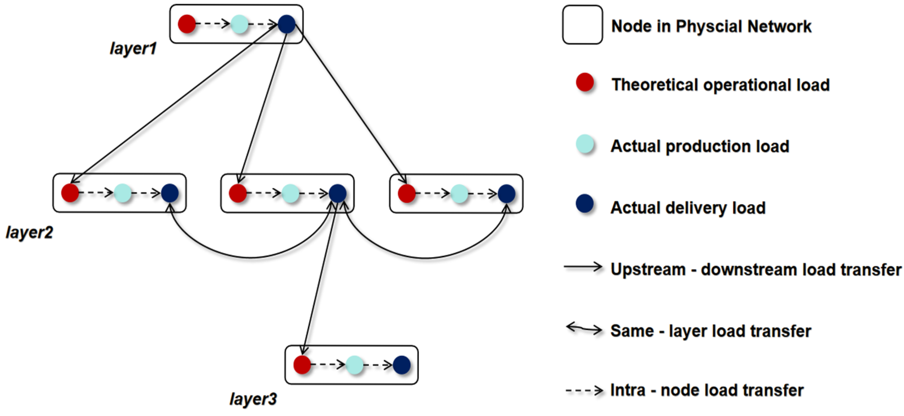
We define S L i α ( t ) as the theoretical operational load representing the load received by node V i P from its upstream nodes at time t ; this also corresponds to the production load under normal conditions. S L i β ( t ) denotes the actual production load, reflecting the actual output of node V i P at time t after accounting for its internal operational efficiency. S L i N ( t ) is the transferred load, representing the amount of load passed to node V i P from other nodes at the same tier at time t . S L i γ ( t ) denotes the actual delivery load, representing the load transmitted from node V i P to its downstream nodes at time t .
Figure 2 takes three randomly selected layers from the Physical Network to simply demonstrate the flow relationships between different types of loads. Specifically, the transferred load, as it represents a relative quantity relationship of transfer (and reception) and is already embedded in the actual delivery load within the calculation logic, is not visualized separately in the figure.
The relationship between load and operational efficiency is described as follows:
Y i ( t ) = S L i β ( t ) / S L i α ( t ) S L i β ( t ) + S L i N ( t ) = S L i γ ( t ) .
Here, we define the initial operational efficiency as Y i 0 = 100 % . For any pair of nodes with an upstream–downstream business relationship, the edge weight is used as the proportional basis for load allocation. Specifically, the edge weight reflects the strength of the business relationship between the entities, and this relationship corresponds to the logistics flow in production-oriented supply chains.
Let Q i , j ( t ) denote the load mapping term from node V i P to node V j P at time t , and Q j , i ( t ) denote the corresponding mapping from node V j P to node V i P . These quantities reflect the structural association of loads between business-related nodes, rather than a conserved physical flow. Here, V j P is an upstream node of V i P with an established business relationship. Let φ i U and ϕ i U denote the sets of upstream and downstream nodes of node V i P , respectively. Let o 1 and o 2 be index variables such that V o 1 P φ i U and V o 2 P ϕ i U . Other set notations follow similar definitions.
To determine the numerical values of Q i , j ( t ) and Q j , i ( t ) , we adopt a proportional allocation mechanism based on the structural connection weights and the relative load level of each node.
Specifically, the mapping from a node to its upstream or downstream neighbors is distributed in proportion to their respective connection weights w i , j P ( t ) and the normalized structural loads. This allocation framework captures how business-related loads are structurally transmitted across the network, and is formally expressed as follows:
Q i , j ( t ) = w i , j P ( t ) V o 1 P φ i U w o 1 , i P ( t ) S L i α ( t ) Q j , i ( t ) = w i , j P ( t ) V o 4 P ϕ j U w j , o 4 P ( t ) S L j γ ( t ) .
This study introduces the concept of relative resistance to load fluctuation, which captures the asymmetric capacity of interconnected nodes to absorb propagated disturbances. In supply chain networks, fluctuations in load between business-related nodes are inherently transmissible, yet the ability to resist such fluctuations is often uneven. Generally, nodes with heavier loads tend to have more suppliers and customers, diversified resource channels, and greater redundancy, enabling stronger buffering and load dispersion. In contrast, lightly loaded nodes typically have limited resources and higher dependency, making them more vulnerable to upstream fluctuations and more likely to amplify cascading effects.
To quantify this disparity, we define R i , j ( t ) as the resistance capacity of node V j P against load fluctuation from node V i P at time t . This reflects the relative load-bearing relationship between the two connected nodes and is expressed as follows:
Q i , j ( t ) = Q j , i ( t ) × R i , j ( t ) Q j , i ( t ) = Q i , j ( t ) × R j , i ( t ) .
The initial Physical Network at this stage satisfies the following relationship:
S L i α ( 0 ) = S L i S L i γ ( 0 ) = S L i β ( 0 ) = S L i S L i α ( 0 ) = V o 1 P φ i U w o 1 , i P ( t ) R i , o 1 ( t ) V o 6 P ϕ o 1 U w o 1 o 6 P ( t ) S L o 1 γ ( 0 ) S L i γ ( 0 ) = V o 2 P ϕ i U w i , o 2 P ( t ) R i , o 2 ( t ) V o 7 P φ o 2 U w o 7 , o 2 P ( t ) S L o 2 α ( 0 ) .
In the physical layer of the supply chain network, node load capacity is limited. Specifically, each node has functional constraints such as supply capacity, manufacturing capability, or sales volume, which result in a defined upper bound for processing or output. These constraints typically show a linear relationship with the node’s initial load level. Meanwhile, the core goal of supply chain nodes is to operate profitably. When product demand declines, raw material supply is disrupted, or profit margins fall below the break-even point, a node may experience operational difficulties and ultimately withdraw from the network.
Therefore, the lower bound of node load reflects the economic feasibility threshold determined by market demand, supply conditions, and cost–revenue balance. If a node’s business volume falls below this threshold, it is more economical to suspend operations. Based on this, nodes must maintain at least a minimum level of load to ensure sustainable operations and to support the overall stability of the supply chain network. We define the upper and lower bounds of node load as S L i ( m a x ) and S L i ( m i n ) , respectively, which are expressed as follows:
S L i ( max ) = α × S L i S L i ( min ) = β × S L i .
Here, the parameter α ( α 1 ) represents the upper bound coefficient of node load, while β ( 0 β 1 ) denotes the lower bound coefficient. Theoretical operational load, actual production load, and final delivery load are all required to remain within the specified load bounds.

2.1.2. Physical Network Cascading Failure Process

In the physical network of a supply chain, the load status of nodes plays a critical role in determining overall system stability and operational efficiency. Node failures are typically categorized into underload and overload failures, which often interact in real-world operations to form complex feedback loops. Underload failure refers to economic or efficiency disruptions caused when a node’s load falls below its lower threshold, often due to production halts or resource shortages. This may prevent the node from receiving materials or fulfilling deliveries, thereby affecting upstream and downstream nodes. Overload failure, on the other hand, occurs when a node’s load exceeds its maximum capacity, potentially leading to decreased efficiency, delayed deliveries, or even system breakdown. These two failure types are often interlinked through load redistribution, forming a chain-reaction mechanism of “failure–redistribution–subsequent failure.” For example, during the COVID-19 pandemic, some contract manufacturers were forced to shut down due to a sudden drop in orders (underload), causing a surge in demand at core enterprises (overload). Similarly, during major e-commerce sales events, some nodes experienced underload due to overstocking, while subsequent changes in product flow led to overloading and failure in other nodes—an illustrative case of interactive failure dynamics.
When overload occurs, the excess load must be redistributed [34]. Prior research shows this process can escalate failures across the system. This study focuses on two redistribution strategies. For underload failure, load transfer typically occurs vertically—toward upstream or downstream nodes—rather than horizontally across peer nodes. This is because vertical transfer allows other stages of the supply chain to absorb the imbalance more flexibly through adjustments in production, inventory, or order levels. Horizontal redistribution, in contrast, tends to induce instability, increase coordination costs, and challenge system balance. As a result, vertical underload redistribution better supports supply chain resilience and operational continuity while minimizing resource disruption and inefficiency. Specifically, when a node fails due to underload, the resulting load deficiency is propagated both upstream and downstream. Taking node V i P as an example, we first examine the upstream propagation process of the underload. This transmission mechanism not only helps alleviate the pressure on the failed node but also enables rational redistribution of the load across hierarchical tiers of the supply chain, thereby maintaining overall system stability and efficiency. The propagation process is as follows:
Stage One: The underload generated at node V i P is propagated upstream:
Δ S L i α ( t ) =   S L i α ( t ) S L i α ( t 1 ) = V o 1 P φ i U Q i , o 1 ( t ) Q i , o 1 ( t 1 ) = V o 1 P φ i U ( R o 1 , i ( t ) × Δ S L o 1 , i γ ( t ) ) Δ S L u 1 , i γ ( t ) = Δ S L i α ( t ) × R i , u 1 ( t ) × Q i , u 1 ( t 1 ) / V o 1 P φ i U Q i , o 1 ( t 1 ) = Δ S L i α ( t ) × R i , u 1 ( t ) × w i , u 1 ( t ) V o 1 P φ i U w i , o 1 ( t ) S L u 1 γ ( t ) = S L u 1 γ ( t 1 ) Δ S L u 1 , i γ ( t ) = S L u 1 γ ( t 1 )   Δ S L u 1 γ ( t ) S L u 1 β ( t ) = S L u 1 β ( t 1 ) + Δ S L u 1 , i γ ( t ) S L u 1 α ( t ) = S L u 1 β ( t ) / Y u 1 ( t ) Δ S L u 1 α ( t ) = S L u 1 α ( t ) S L u 1 α ( t 1 ) Q i , u 1 ( t ) = Q i , u 1 ( t 1 ) Δ S L u 1 , i γ ( t ) × R u 1 , i ( t ) .
Here, all alphabetic symbols follow a consistent notation convention. For example, Δ S L i α ( t ) represents the change in theoretical operational load of node V i P at time t , while Δ S L o 1 , i γ ( t ) denotes the actual load variation received by node V o 1 P from node V i P at time t .
Stage Two: We model the impact of the failed node V i P on its directly connected downstream node V d 1 P as follows:
Δ S L i β ( t ) × S L i γ ( t 1 ) S L i β ( t 1 ) = Δ S L i γ ( t ) Δ S L i γ ( t ) = S L i γ ( t ) S L i γ ( t 1 ) = V o 2 P ϕ i U Q i , o 2 ( t ) Q i , o 2 ( t 1 ) = V o 2 P ϕ i U ( Δ S L o 2 , i α ( t ) × R o 2 , i ( t ) ) Δ S L d 1 , i α ( t ) = Δ S L i γ ( t ) × R i , d 1 ( t ) × Q i , d 1 ( t 1 ) / V o 2 P ϕ i U Q i , o 2 ( t 1 ) = Δ S L i γ ( t ) × R i , d 1 ( t ) × w d 1 , i P ( t ) V o 2 P ϕ i U w o 2 , i P ( t ) S L d 1 α ( t ) = S L d 1 α ( t 1 ) Δ S L d 1 , i α ( t ) = S L d 1 α ( t 1 ) Δ S L d 1 α ( t ) S L d 1 β ( t ) = S L d 1 α ( t ) × Y d 1 ( t ) S L d 1 γ ( t ) = S L d 1 β ( t ) × S L i γ ( t 1 ) S L i β ( t 1 ) Δ S L d 1 γ ( t ) = S L d 1 γ ( t ) S L d 1 γ ( t 1 ) Q i , d 1 ( t ) = Q i , d 1 ( t 1 ) Δ S L d 1 , i α ( t ) × R d 1 , i ( t ) .
Here, all variables follow consistent notation conventions. For example, Δ S L O 2 , i α ( t ) denotes the theoretical operational load variation at node V o 2 P at time t , as influenced by node V i P .
In real-world supply chain systems, node anomalies are not always localized; under the influence of internal and external factors, they may trigger large-scale anomaly propagation. In traditional load–capacity models, load variations are typically assumed to be linearly additive. However, in load propagation models based on actual logistics networks, the transmissibility of logistics volume can lead to more complex forms of load superposition or conflict. Specifically, these phenomena can be categorized into two types:
1. Load Fluctuation Superposition
When two adjacent upstream and downstream nodes experience simultaneous anomalies, the process of load propagation may exhibit an additive effect. For instance, let Q j , i ( t ) represent the load flow between node V i P and its neighboring node V j P at time t . When node V i P fails, the flow received by V j P decreases, leading to a reduction in Q j , i (t). If node V j P also undergoes a reduction in its own load level Q j , i ( t ) , the effect of the failure at node V i P aligns with the load reduction at node V j P , and the two effects reinforce one another.
Once the propagation caused by the failure of V i P is completed, the influence of both V i P and V j P on the entire network is fully realized, allowing the system to reach a coordinated state. From a systemic perspective, the failure-induced load propagation from node V i P and the concurrent reduction in load at node V j P can be considered as a unified response. This integrated effect completes the redistribution process automatically by the end of the propagation phase.
2. Load Fluctuation Contention
In some scenarios, simultaneous load-increasing and load-reducing demands may create adjustment conflicts. Load-reducing demands, often due to capacity limits or market fluctuations, are reactive and hard to adjust. In contrast, load-increasing demands aim to enhance efficiency and provide greater flexibility. When both occur along the same path, load-increasing demands are often suppressed due to limited resources or a slow system response, which complicates load redistribution and challenges system stability. Under such superposition and conflict conditions, centralized supply chain structures can coordinate load balancing more effectively during multi-failure fluctuations, allowing conflicting objectives among supply chain participants to be reconciled through integrated mechanisms [35,36]. The following section outlines the steps of the propagation process:
Step 1: Node-Level Load Self-Balancing
When the load of a node fluctuates within the network, the system first performs a structural adjustment based on the internal coupling relationships among multiple types of loads within that node (see Equation (6)). These load types are subject to fixed proportions or internal balancing mechanisms; therefore, when one type of load changes, the others will automatically adjust in response according to the established relationship.
Step 2: Propagation of Load Variation from Supplier Nodes
For simplification, let S L i N t = 0 , and assume S L i β t = S L i γ t . All nodes within the Physical Network are internally coordinated.
After coordination, suppose that at time t , there are n supplier nodes experiencing a reduction in S L i γ t , with variation magnitudes denoted as S L i γ t . According to Equation (12), the load variation propagates downstream to the manufacturing tier (M), the distribution tier (D), and the retail tier (R).
For the downstream node V j P , we consider the variations in S L j α t and S L j γ t . Since S L j γ t = S L j β t , we focus only on the changes in S L j γ t .
The variation in node V j P caused by the fluctuation in the supplier node V i P is represented by two virtual load variation terms, denoted as V S L j , i α t and V S L j , i γ t , where the α , β and γ correspond to different load types as defined earlier (representing theoretical operational load, actual production load, and actual delivery load, respectively). These virtual terms are used for intermediate calculations during the load adjustment process and do not actually alter the real-time load values of the nodes.
X j α ( t ) = V i P φ j U Δ V S L j , i α ( t ) X j γ ( t ) = V i P φ j U Δ V S L j , i γ ( t ) .
Here, X j α ( t ) and X j γ ( t ) are cumulative intermediate metrics that quantify the aggregated effect of upstream virtual load variations on the downstream node V j P . They serve as key inputs for the subsequent load adjustment equations, helping to systematically translate upstream disturbances into actionable load change signals for the node.
Step 3: Load Adjustment Rule for the Manufacturing tier
In the manufacturing tier, the load fluctuation of each node’s S L j γ t is denoted as Δ V S L j γ t , representing the level of disturbance experienced by the manufacturing node at time t . According to the load propagation rule, we have X j γ ( t ) < 0 . The temporal transition equations for Δ V S L j γ t and X j γ ( t ) are as follows:
  ( X j γ ( t )   , Δ V S L j γ ( t ) ) =   ( X j γ ( t ) Δ V S L j γ ( t ) , 0 ) , Δ V S L j γ ( t ) > 0 ( 0 , Δ V S L j γ ( t ) X j γ ( t ) ) , Δ V S L j γ ( t ) < X j γ ( t ) 0   ( X j γ ( t ) Δ V S L j γ ( t ) , 0 ) , X j γ ( t ) < Δ V S L j γ ( t ) < 0 ( 0 , 0 ) , X j γ ( t ) = Δ V S L j γ ( t ) .
Step 4: Upstream and Downstream Load Propagation
After adjustment, if the load fluctuation Δ V S L i γ t of any node in the manufacturing tier is nonzero, the internal coupling mechanism will trigger changes in Δ V S L i α t , propagating the disturbance upstream to the supplier tier (S) and directly downstream to the distribution tier (D) and retail tier (R). Once propagation is completed, similar to Equation (13), the cumulative values of X j α ( t ) and X j γ ( t ) for all nodes in the network are computed.
Step 5: Load Adjustment in the Distribution and Retail Tier
For load variations occurring at nodes in the distribution tier (D) and the retail tier (R), the system continues the iterative propagation–adjustment process by repeating Steps 2 and 3. This process iterates continuously and propagates across the entire network until all nodes reach a new steady-state load distribution.
Step 6: Update of All Node Loads
After the above propagation process, the load of each node is finally adjusted based on the aggregated load variation. For each node, its final load value is calculated using the following equation:
S L j α ( t + 1 ) = S L j α ( t ) + X j α ( t ) S L j γ ( t + 1 ) = S L j γ ( t ) + X j γ ( t ) .
Through the above propagation and adjustment process, the load states of all nodes are synchronously updated, and the resulting values represent the final system state under the current round of disturbance propagation.

2.1.3. Overload Reallocation Mechanism for Nodes in Centralized Supply Chain Physical Networks

In centralized supply chain environments, intra-tier reallocation remains the priority strategy for rapid system stabilization when a node experiences load overload. These nodes, being similar in function, enable fast adjustment with minimal loss. If that fails, the system escalates the excess to downstream nodes, forming a secondary chain of failure. In a centralized supply chain structure, rapid intra-tier reallocation is the optimal strategy for responding to abnormal disruptions. When a node becomes overloaded or nears shutdown, excess load is swiftly transferred to peer nodes within the same tier—nodes that share similar equipment, logistics processes, and resource configurations—minimizing overall impact and ensuring continued operation. If that tier’s reallocation capacity is exhausted, surplus load cascades downstream, risking further failures.
In centralized supply chain structures, when a node experiences severe overload—such as due to labor shortages, equipment limitations, or physical bottlenecks—its processing capacity may significantly decline, potentially leading to production interruptions. The subsequent state of the node is characterized by three probabilistic outcomes: with probability P 1 , the node collapses completely; with probability P 2 , the node remains functional but operates at reduced efficiency, quantified by λ ( 0 , 1 ) , where a bigger λ indicates greater capacity loss; with the remaining probability 1 P 1 P 2 , the overloaded node remains stable within its capacity boundary. When load is redistributed within the same tier, the nodes are assumed to be homogeneous, and their load tolerance coefficient is set to 1.
Let the set of overloaded nodes be defined as V 1 = V i P i 1 ,   2 ,   3 ,   n , and the set of redundant nodes capable of absorbing excess load be defined as V 2 = V j P j n + 1 ,   n + 2 , n + 3 ,   m . Here, Δ D S L i ( t ) denotes the actual delivery load required by node V i P , and Δ R S L i ( t ) denotes the actual delivery load output by redundant node V j P . The corresponding formulation is given as follows:
Δ D S L i ( t ) = ( S L i α ( t ) S L i ( max ) ) × Y i ( t ) Δ R S L j ( t ) = ( S L j ( max ) S L j α ( t ) ) × Y j ( t ) .
The state transition equation for the redundant node V j P is given as follows:
Δ S L i , j γ ( t ) = Δ R S L j ( t ) j = n + 1 m Δ R S L j ( t ) × Δ D S L i ( t ) Y j   ( t + 1 ) = Y j   ( t ) S L j α ( t + 1 ) = τ S L j ( max ) , i = 1 n Δ D S L i ( t ) > τ j = n + 1 m Δ R S L j ( t ) S L j α ( t ) + Δ S L i , j γ ( t ) Y j ( t + 1 ) , i = 1 n Δ D S L i ( t )   τ j = n + 1 m Δ R S L j ( t ) S L j γ ( t + 1 ) = S L j γ ( t ) S L j β ( t + 1 ) = S L j α ( t + 1 ) Y j   ( t + 1 ) S L j γ ( t + 1 ) = S L j β ( t + 1 ) + S L j N ( t + 1 ) .
Here, S L i , j γ ( t ) represents the load received by node V i P from node V j P at time t , while S L j , i γ ( t ) denotes the load transferred from node V j P to node V i P . These two terms form a pair of forward and reverse reflections of the load transfer, satisfying the conservation relationship:
Δ S L i , j γ ( t ) = Δ S L j , i γ ( t ) .
The received load is recorded as a positive value, while the transmitted load is recorded as negative. To prevent instability during resource reallocation, a resource redundancy safety threshold τ is set. When the total requested load exceeds this threshold, the system prioritizes proportional allocation based on maximum tolerance. In this study, τ is set to 95%.
S L i α ( t + 1 ) = 0   , with   probability   P 1   S L i ( max )   , with   probability   1 P 1   Y i ( t + 1 ) = 0   , with   probability   P 1 Y i ( t ) ( 1 λ )   , with   probability   P 2 Y i ( t )   , with   probability   1 P 1 P 2 S L i γ ( t + 1 ) = 0 , with   probability   P 1 f i ( t + 1 ) , with   probability   1 P 1 f i ( t + 1 ) = S L i γ ( t ) , i = 1 n Δ D S L i ( t ) τ j = n + 1 m Δ R S L j ( t ) S L i α ( t + 1 ) × Y i ( t + 1 ) + ( S L i α ( t ) S L i ( max ) ) × τ j = n + 1 m Δ R S L j ( t ) i = 1 n Δ D S L i ( t ) , otherwise S L i β ( t + 1 ) = S L i α ( t + 1 ) Y i ( t + 1 ) S L i γ ( t + 1 ) = S L i β ( t + 1 ) + S L i N ( t + 1 ) .
The state transition equation for the overloaded node V i P is given as Equation (19). The equation describes the dynamic load adjustment mechanism under centralized control when node overload occurs in the network. After load reallocation is completed, if any new node exceeds its upper bound or falls below its lower bound, the system will repeat the above process until the load of all nodes stabilizes within the predefined threshold range. Parameter explanations are as follows: the operational efficiency degradation coefficient is denoted by λ = 20 % ; the complete failure probability of a node is set as P 1 = 30 % ; and the threshold for operational efficiency degradation is defined as P 2 = 30 % .

2.2. Information and Decision Risk Network

In the coupled network constructed in this study, the Information and Decision Risk Network comprises two functionally complementary subnetworks: the Communication System Network, which characterizes the communication structure for information acquisition, transmission, and response among nodes, with its topology determining propagation efficiency through edge weights (bandwidth/latency/reliability); and the Decision Risk Network, which captures the propagation of decision uncertainty arising from information asymmetry, delays, or prediction biases. These subnetworks, while structurally independent, are functionally interconnected: the Communication System transmits information while the Decision Risk Network propagates uncertainty. By modeling these two categories of non-physical pathways, this research allows for a comprehensive analysis of cascading failure mechanisms under complex disturbances.

2.2.1. Communication System Network Load and Constraint Model

The Communication System Network, as a complex system involving multi-component collaboration, carries key functions such as information collection, input, transmission, and feedback. These components work in coordination to support the generation, storage, processing, transformation, transmission, and reception of signals and data [37]. This network encompasses not only the physical layer of communication infrastructure—such as storage devices, routers, switches, and base stations—but also the protocol layer mechanisms for scheduling and optimization, which together ensure the high efficiency and reliability of data transmission.
In the supply network model, all functional communication devices are represented as nodes, and the data transmission media between devices are modeled as links. Let the Communication System Network at time t be denoted as G t C ( V t C , E t C , W t C ) , where V t C = ( V 1 C , V 2 C V n C ) represents the set of communication nodes. Among them, N t C ( r e g u l a r ) is the set of regular nodes, and N t C ( f o c a l ) is the set of focal nodes. The edge set is defined as E t C = ( V i C , V j C , e i j C ( t ) | e i j C { 0,1 } , i , j = 1 , 2 , 3 n } , which indicates the presence of communication links between devices at time t . Specifically, if e i j C ( t ) = 1 , it means that node V i C and node V j C are connected; otherwise, if e i j C ( t ) = 0, they are not connected. The weight set is defined as w t C = { w i , j ( t ) | i , j = 1 , 2 , 3 n } , where w i , j C ( t ) represents the communication delay, cost, or path difficulty between node V i C and node V j C at time t . In distributed network systems, each node continuously generates and receives data packets at a constant rate while simultaneously executing routing functions. To ensure high network transmission efficiency, routing protocols often require that data be transmitted along the shortest paths—meaning that the shorter the path length, the higher the transmission efficiency.
To assess the burden and information flow within the network, the concept of betweenness centrality (BC) is commonly used [38]. One approach is to link a node’s load to its betweenness centrality, based on the assumption that nodes lying on shorter paths between other nodes tend to bear more traffic [39,40]. Under this centrality-based modeling framework, a node’s load capacity is typically proportional to its initial betweenness centrality. When a node fails, it may cause the redistribution of traffic across the network. Importantly, this redistribution does not necessarily affect the node’s immediate neighbors but can impact any node that lies along new rerouted shortest paths.
Based on this modeling rationale, we define the initial load of a network node. Let D i , j ( t ) denote the shortest path length from node V i C to node V j C at time t , expressed by the following formula:
D i , j ( t ) = min { w i , k 1 C ( t ) + w k 1 , k 2 C ( t ) + + w k n , j C ( t ) } .
The sequence { k 1 , k 2 , k 3 k n } represents the indices of intermediate nodes along a valid path from node V i C to node V j C ; the edge weight w i , j C ( t ) is defined as follows:
w i , j C ( t ) = [ d i C ( t ) × d j C ( t ) ] σ .
The weight parameter is set as σ = 0.5 . Further based on the theory of dynamic betweenness centrality, the information load M L i ( t ) of node V i C is defined as equal to its dynamic betweenness centrality B C i ( t ) :
M L i ( t ) = B C i ( t ) = V i C ( t ) , V j C ( t ) , V k C ( t ) V t C , i j k θ i , j k ( t ) θ i , j ( t ) .
Under this definition, θ i , j ( t ) represents the total number of shortest paths from node V i C to node V j C , while θ i , j k ( t ) denotes the number of shortest paths from node V i C to node V j C that pass through node V k C . Unlike traditional assumptions where all initial edge weights are set to 1, this study considers edge heterogeneity in the initial state to better reflect the actual operating conditions of equipment and the underlying structure of routing.
The maximum buffer capacity for information at a node operating at normal efficiency is defined as M L i ( m a x ) , and the external decision request volume that can be temporarily stored is M L i m a x M L i ( 0 ) , where M L i ( 0 ) is the initial information load of the node. Furthermore, it is assumed that the maximum buffer capacity is proportional to the initial load, as follows:
M L i ( max ) = α 2 M L i ( 0 ) .
The parameter α 2 represents the information buffering capacity of the node.

2.2.2. Communication System Network Cascading Failure Process

When a node V i C satisfies M L i ( t ) > M L i ( m a x ) at time t , buffer overflow occurs. In most prior studies, such nodes are usually directly removed. However, this study presents a different viewpoint: node overload does not directly lead to node failure. Instead, it manifests as localized congestion. This is because the data transmission load of enterprise equipment does not propagate between nodes but results in internal queuing. Specifically, when the load M L i ( t ) of node V i C exceeds its maximum capacity M L i ( m a x ) , it manifests in practice as information loss or decision delay. This further appears in the network as increased transmission latency. Congestion affects neighboring nodes by slowing their processing rates, thus indirectly increasing their buffer pressure and forming a feedback loop. Specifically, when the load of node V i C exceeds the threshold, the edge weight w i , j C ( t ) between node V i C and V j C increases relative to its initial weight w i , j C ( 0 ) , indicating greater transmission difficulty. The edge weight update rule is defined as follows:
w i , j C ( t ) = w i , j C ( 0 ) M L i ( t ) M L i ( max ) .
If at time t , the load of node V i C satisfies M L i ( t ) M L i ( m a x ) , then the weight of the edge between nodes V i C and V j C remains unchanged. Based on this condition, we derive the following expression:
w i , j C ( t + 1 ) = w i , j C ( 0 ) M L i ( t ) M L i ( max ) , M L i ( t ) > M L i ( max ) w i , j C ( 0 ) , otherwise .
When a node in the communication network fails, the network load is redistributed. The evolution of the shortest path is a direct result of dynamic changes in edge weights. During each round of propagation iteration, the system updates the shortest paths d i , j ( t ) between all node pairs based on the current w t C , using algorithms such as Dijkstra or Floyd–Warshall. It then recalculates the shortest path count θ i , j ( t ) , path occupancy θ i , j K ( t ) , and adjusts the evolving betweenness centrality B C i ( t ) of nodes to reallocate node loads.
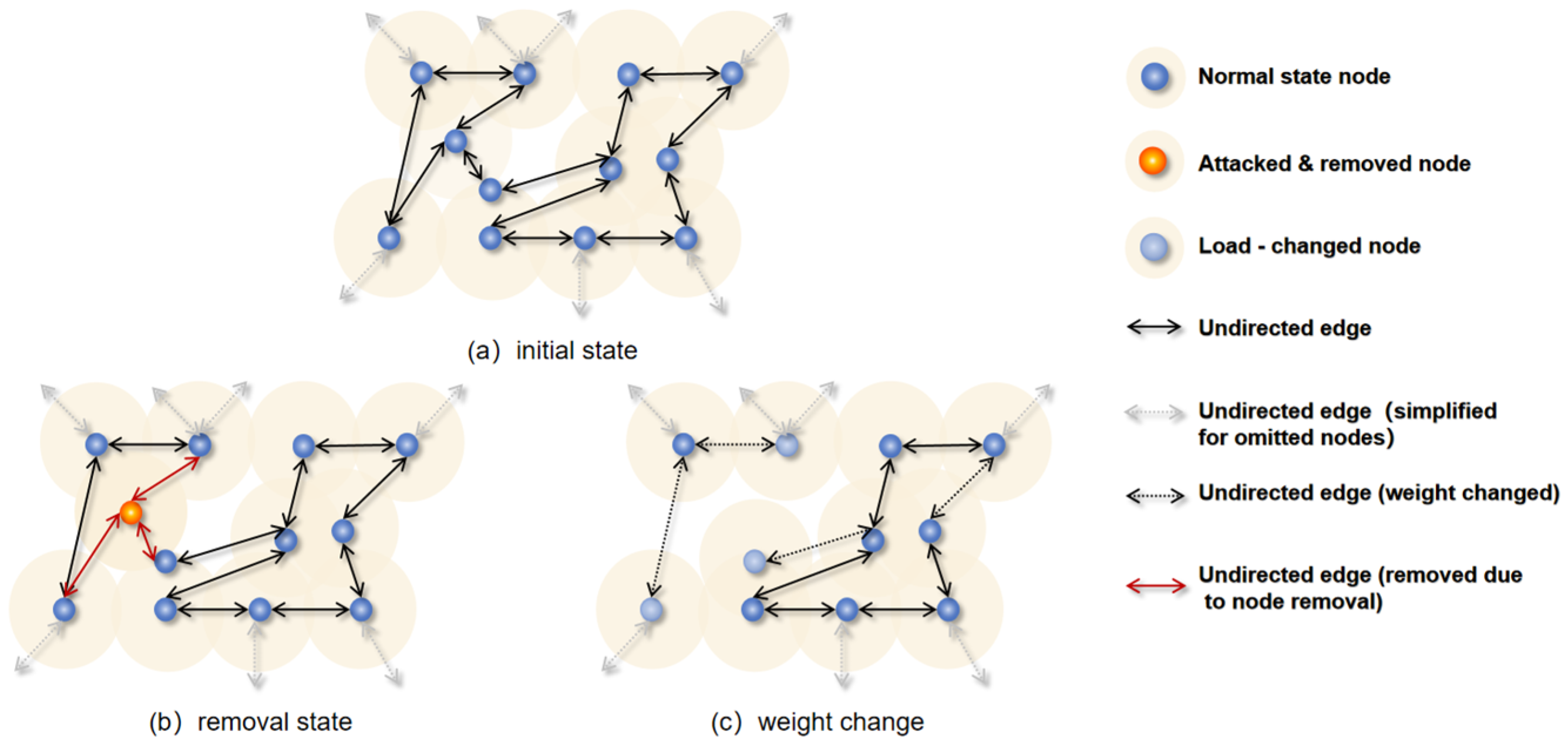
Figure 3 illustrates the evolution process during a single round of weight adjustment.
Specifically, changes in edge weights increase the instability of the network, potentially causing failures to propagate across the system. This type of diffusion may trigger cascading failures where the failure of a node or edge causes additional nodes or edges to fail, initiating a new round of dynamic load adjustments. This process may continue until the network reaches a new steady state or triggers a system-wide cascading breakdown.

2.2.3. Decision Risk Network Load and Constraint Model

In traditional supply chain information networks, enterprise decisions are often treated as isolated actions, with little attention paid to how decision risks spread. However, in today’s highly collaborative supply chains, decisions are interdependent, and risks propagate along information chains. This study proposes the Decision Risk Network, a novel model that captures how enterprise decisions are shaped by others’ inputs and how decision risks propagate dynamically.
Each firm’s decision-making relies on the quality of the received information. Factors like source complexity, completeness, timeliness, decision-makers’ capabilities, frameworks, and external uncertainties contribute to risk formation and transmission [41]. This networked view transforms supply chain decision-making into a dynamic risk propagation process.
1. Network Characteristics of Decision Risk
Decision risk propagation structurally mirrors information diffusion models [42]. In the network, nodes represent firms, and weighted edges reflect business dependency. Risks spread bidirectionally—affected by both upstream suppliers and downstream clients—necessitating undirected weighted networks to capture symmetric transmission. Unlike material flows, decision risks follow paths shaped by collaboration, requiring models that combine directional information flow with reciprocal risk dynamics.
2. Centralization in Decision Risk Network
Decision risk networks often show high centralization. Focal nodes—such as strategic suppliers—hold top positions in centrality metrics and influence capacity planning, standard-setting, and order dispatching. This creates a star-shaped structure where core failures can reduce system efficiency by 30–50% [43] and trigger cross-domain collapses. Given their high influence, uncontrolled risks at these nodes can destabilize the entire supply chain.
3. Cascading Failure of Decision Risk
Lack of timely, accurate decisions increases information asymmetry and uncertainty, impairing coordination and causing cascading failures. Nodes that fail to share reliable forecasts disrupt downstream planning, while delayed logistics responses create mismatches between material and information flows.
This study models this cascade: focal node failures lead to exponential decision delays at connected nodes, potentially triggering further breakdowns. The spillover risk is proportional to the core node’s network control scope. Accumulated distortions may cause a domino effect, destabilizing the supply chain. Unlike classical rumor or virus models—which assume instantaneous spread—this study, grounded in energy release theory, adopts a capacity–load framework combined with disaster dynamics modeling, treating risk as quantifiable energy to simulate its gradual accumulation and propagation.
The Decision Risk Network is defined as G t D ( V t D , E t D , w t D ) , where V t D = V 1 D , V 2 D V n D denotes the set of virtual nodes in the network, with N t D r e g u l a r representing the set of regular nodes and N t D f o c a l representing the focal nodes. The edge set is given by E t D = ( V i D , V j D , e i j D t e i j D 0,1 , i , j = 1 , 2 , 3 n , where e i j D = 1 indicates a connection between V i D and V j D , and e i j D = 0 otherwise. The weight set is defined as w t D = w i , j t i , j = 1 , 2 , 3 n , where w i , j D t denotes the connection weight at time t between nodes V i D and V j D , quantifying their decision risk propagation capacity in terms of business association intensity (such as order ratio, technological dependence, and contractual constraint strength). In supply chain networks, there exists a positive correlation between the initial decision risk load and decision-making strength, which is determined by three key dimensions: the number of information sources, the complexity of business operations at production nodes, and the burden of communication; more specifically, (1) Information Resource Quantity: Decision-making capability is positively correlated with the amount of information resources and can be quantified by the degree metric of nodes in the Decision Risk Network. (2) Production Business Complexity: Represented through the initial comprehensive load in the Physical Network. (3) Communication Load: Determined by the load capacity of all nodes in the Communication System Network connected to the given node.
To maintain consistency with the production load calculation method, this study adopts a matrix construction approach similar to that used in the Physical Network and builds a non-negative matrix factorization model. We obtain the matrix V D :
V D = d i D ( 0 ) S L i V o 9 D ε i U M L o 9 ( 0 ) d j D ( 0 ) S L j V o 10 D ε j U M L o 10 ( 0 ) d n D ( 0 ) S L n V o 11 D ε n U M L o 11 ( 0 ) .
Here, all alphabetic symbols follow a consistent notation convention. Let d i D t represent the degree value of decision processing node V i D at time t in the decision processing network. The set ε i U represents all nodes in the Decision Risk Network that are connected to node V i D , and M L o 9 0 denotes the initial load value of node V o 9 C in the Communication System Network corresponding to node V o 9 D .
To ensure uniform contribution values of all elements to the matrix, the data has been normalized. The matrix is now decomposed, with the latent feature dimension set as r = 1 to extract the latent feature value of the nodes, where
V D = W D × H D .
Each value of W D , denoted as F e a t u r e i D , represents a latent feature value. We define the self-imposed decision risk load of a node as S H L i ( t ) . When its connected nodes fail, the node receives additional decision risk load A H L i ( t ) . The total decision risk load of each node is denoted as H L i ( t ) , which is expressed as
H L i ( t ) = S H L i ( t ) + A H L i ( t ) .
At the initial moment, the self-imposed decision risk load of node S H L i ( 0 ) = F e a t u r e i D , and the initially received decision risk load is A H L i ( 0 ) = 0 . The upper limit of the load at a decision network node represents the enterprise’s risk preference. The maximum load capacity is defined as
H L i ( max ) = α 3 H L i ( 0 ) .
Here, α 3 represents the risk tolerance coefficient of the network node. The larger the coefficient, the more aggressive the enterprise’s risk preference, and α 3 > 1 .

2.2.4. Decision Risk Network Cascading Failure Process

Based on the disaster propagation dynamics model [44], this study constructs a decision risk propagation model by incorporating the structural characteristics and behavioral mechanisms of risk transmission in supply chains. The model assumes that when a node’s risk load exceeds its maximum tolerance threshold, it will trigger a functional disruption, and the risk load of the failed node will be transferred to its neighboring nodes. If the accumulated load of the receiving node continues to exceed its threshold, it will lead to cascading failures. This model not only retains the logical foundation of disaster models but also integrates real-world features of supply chains such as information delays, risk amplification, and structural coupling. The model is as follows:
A H L j ( t + 1 ) = A H L j ( t ) + ψ ( H L i ( t ) × w i , j D ( t ) × Θ ( d i D ( t ) ) × e μ Δ t V o 9 D ε i U w i o 9 D ( t ) ) + ξ j ( t ) H L j ( t + 1 ) = S H L j ( t + 1 ) + A H L i ( t ) .
The expression for w i , j D ( t ) is given as
w i , j D ( t ) = [ d i D ( t ) × d j D ( t ) ] σ
where σ = 0.5 .
The transmission of risk between enterprises is influenced not only by the strength of inter-enterprise relationships but also by the total number of partners each enterprise has. Therefore, the risk ultimately received by an enterprise is not merely the sum of the risks from all transmitting enterprises. In this paper, the second term on the left-hand side of the first line of Equation (30) quantifies the variation in the risk burden of enterprise node V j D caused by its neighboring infected enterprises transmitting risk. The function ψ x , analogous to an S-shaped function used in neural networks, is introduced to model the portion of risk transmitted by neighboring enterprises and received by enterprise V j D . Its mathematical expression is given by
ψ ( x ) = 1 e γ x 1 + e γ ( x H L i ( max ) ) .
As shown in Equation (32), the function attenuates the influence of external risk on V j D . Specifically, when x = 0 , regardless of the values of γ and H L i ( m a x ) , it results in ψ x = 0 . This implies that a normal enterprise node does not transmit risk to others. In this paper, the parameter is set as γ = 10 , which provides a reasonable trade-off between the smoothness of response and the sharpness of transition around the risk threshold.
The function Θ ( d j D t ) represents the degree function of node V i D , reflecting the extent to which an infected node impacts its neighboring enterprises. The expression is given as
Θ ( d j D ( t ) ) = 1 + b × d j D ( t ) a × d j D ( t ) .
The higher the degree, the more connections node V i D has within the network, which means it transmits risk to more neighboring enterprises. Consequently, the amount of risk it can receive also increases. Here, a and b are constants in the function Θ ( d j D t ) , and for the simulation, based on relevant prior research, we take a = 4 , b = 3 .
e μ is the risk amplification factor during the transmission process, originally expressed as e μ t , representing the exponential increase in risk as it spreads from node V i D to V j D . When node V j D faces long-term uncertainty or lacks confirmed information, it is more prone to panic-driven decisions, thereby increasing the amount of risk it receives from node V i D . Since this paper adopts a time-discrete approach to simulate the propagation of risk, we set t = 1 , indicating that one unit of time is required to complete a round of transmission. Additionally, μ represents the intensity of risk amplification: the larger the value, the more susceptible the enterprise is to long-term uncertainty, indicating higher potential risk impact. In this paper, we set μ = 1 to simplify the analysis of trends in other variables. This setting does not affect the model’s relative response patterns and helps highlight the dominant role of structural characteristics in system behavior.
In the process of inter-enterprise risk propagation, random changes in internal and external environments may also impact the affected node. These factors may arise from internal business processes within the node’s enterprise, or externally from market fluctuations or environmental volatility, which are often irregular and unpredictable. Therefore, the first term on the right-hand side of the first line of Equation (30) represents the influence of these factors on node V j D during risk propagation and is denoted using the random variable ξ j ( t ) . This variable is typically assumed to follow a normal or uniform distribution. In this paper, it is assumed to follow a uniform distribution:
ξ j ( t ) ~ U ( 0 , Δ u )
where Δ u = 0.001 .

2.3. Asymmetrically Coupled Centralized Supply Chain Network Model

In 2010, Buldyrev et al. first proposed the concept of interdependent networks (referred to as “coupled networks” in this paper) and applied network models [45] to illustrate that mutually dependent networks exert reciprocal impacts. The failure of a node in one network may cause the failure of its corresponding node in the other. A prominent phenomenon is that with changes in the network’s topological parameters, the maximum connected component in the network undergoes a discontinuous phase transition. Such abrupt changes lead to sudden system collapse, and as the number of fully coupled sub-networks increases, this abrupt phase transition becomes more difficult to predict [46].
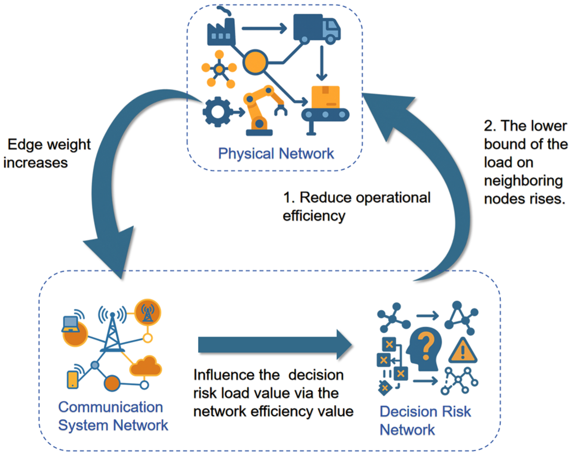
When a disruption or node failure occurs, the delay in information transmission, spread of decision bias, and uncertain responses from production nodes may interact with each other and propagate along the structural dependency paths across the dual-layered networks, triggering systemic cascading failures. To systematically describe this coupling mechanism, this paper treats the Communication System and the Decision Risk Network as a unified functional network, which forms a corresponding coupling relationship with the physical production network. To provide an intuitive overview of the interaction pathways among multi-layer coupled networks, a schematic illustration is presented in Figure 4, which will be elaborated in the following subsection.
Here, we assume that each node in a given layer has a strict one-to-one correspondence with nodes in other networks, denoted as V i P , V i C , V i D .

2.3.1. Coupling Mechanism of Physical Network with Information and Decision Risk Network

When a node in the Physical Network experiences a sudden failure, its load and production status directly affect the load of the Communication System Network. For example, when the load of a production node falls below a threshold and it can no longer plan production, it will increase the communication burden on the equipment network. Specifically, this manifests as having to urgently transmit updated production schedule information downstream, delaying notifications, or adjusting order quantities. Therefore, we set the weight of the corresponding node’s adjacent edges in the Communication System Network to be expanded by a factor of η 1 .
w i , j C ( t ) = η 1 w i , j C ( 0 )
where η 1 represents the coupling coefficient between the Physical Network and the Communication System Network, reflecting the degree of interconnection between them.
When a node in the Decision Risk Network is removed due to risk of overload failure, the interruption of its decision-making function can trigger a system-wide chain reaction. Specifically, this is manifested in the fact that the node’s ability to process real-time information is lost, leading to a significant decline in overall production efficiency indicators (such as response speed and resource allocation accuracy). For the removed node V i D , the efficiency indicator Y i ( t ) of its corresponding node V i P in the Physical Network is reduced to 75% of its original value. Due to the disruption of decision information transmission paths between neighboring nodes, upstream nodes are unable to obtain dynamic demand data to generate production plans in time. As a result, downstream nodes fall into a passive decision-making state due to the lack of inventory adjustment instructions. This increase in information interruption layers raises production risks and expected production costs for upstream and downstream nodes. Consequently, the risk mitigation mechanism is triggered between them to avoid greater losses by increasing production redundancy. The specific formula is as follows:
H E F i ( t ) = H L i ( t ) H L i ( max ) S L j ( min ) = η 2 × S L j ( min ) × H E F i ( t )   , V i D N t D ( regular ) S L j ( min ) = η 2 × η 3 × S L j ( min ) × H E F i ( t ) , V i D N t D ( focal )
where H E F i ( t ) represents the decision risk panic coefficient of the removed node V i D , which measures the extent to which the decision risk status of the node affects the stability of the coupled network system. η 2 is the coupling strength coefficient, used to quantify the coupling intensity between networks; η 3 is the focal node impact multiplier, used to quantify the relative impact of focal nodes compared to ordinary nodes.

2.3.2. Intrinsic Coupling Dynamics of Information and Decision Risk Network

When nodes in the Communication System Network become overloaded, the decision-processing burden of associated nodes in the Decision Risk Network increases. This is because when a node in the Communication System Network is overloaded, its communication efficiency decreases, which in turn raises the decision-processing intensity of its associated nodes. As a result, these nodes must rely on less or inaccurate information to make decisions, thereby increasing decision risk. We define
E j ( t ) = 1 N 1 V i C , V j C V t C , i j 1 d i , j ( t ) S H L i t + 1 = η 4 o 11 ε i U ( E o 11 ( t ) E o 11 ( 0 ) 1 ) × S H L i ( t )
where E j ( 0 ) represents the initial communication efficiency of node V j C in the Communication System Network, and E j ( t ) represents the communication efficiency of node V j C in the Communication System Network at time t . N denotes the number of nodes in the network. η 4 is the coupling coefficient between the Communication System Network and the Decision Risk Network, reflecting the closeness of the connection between the two networks.

3. Numerical Simulation

3.1. Experimental Conditions

The experimental environment in this study is configured as follows: the operating system is Windows 11, the programming language is Python 3.13.0, the CPU used is an AMD Ryzen 7 6800HS with Radeon Graphics at 3.20 GHz, and the memory used is 929 GB.

3.2. Synthetic Networks

Due to the confidential and proprietary nature of most supply chain data, reconstructing complete real-world supply chain networks is highly challenging. Consequently, research from the perspective of complex networks often relies on representative network models, among which random networks and scale-free networks are the most commonly used. This study adopts these two models to construct the Physical Network and the Communication Network, respectively.
Hernández and Pedroza-Gutisamrrez [47] constructed a theoretical Physical Network using a random network model in a bipartite graph. Similarly, for the Physical Network in this study, a synthetic network approach is adopted to construct a four-tier supply chain Physical Network model. Network nodes consist of suppliers, manufacturers, distributors, and retailers, totaling 400 nodes, evenly divided into four tiers. Each enterprise node belongs to only one tier. Links are randomly established between adjacent tiers with a connection probability of 0.1, which represents the likelihood of business relationships between nodes in adjacent tiers.
We assume that the initial production volume (logistics volume) at the retail layer nodes is 60,000. Based on the weight ratios with neighboring business nodes, the initial production volume is assigned to the upstream nodes. For a retail tier node V i P and its upstream neighboring nodes V u 1 P , the allocation P u 1 satisfies the following formula:
P u 1 = V o 12 P ϕ u 1 U w u 1 , o 12 ( 0 ) V o 12 P ϕ u 1 U w u 1 , o 12 ( 0 ) P O 12 .
According to Equation (38), the production volume (logistics volume) of all nodes in the Physical Network is assigned.
For the equipment communication network, we use the Barabási-Albert (BA) model [43] to generate the Communication System Network. In the BA model, nodes are connected based on the principle of preferential attachment—new nodes tend to connect to already well-connected nodes rather than randomly. As a result, the generated network follows a power-law degree distribution. Under this mechanism, some nodes in the network become “hub nodes,” playing important roles in connectivity and information propagation. This characteristic effectively simulates real-world communication networks, making the BA model a suitable choice for communication network simulation in this study. We generate a scale-free network with 400 nodes and an average degree of 2.
For the Decision Risk Network, since decision-making typically targets business relationship entities, we set the topology of the decision-processing network to be identical to that of the Physical Network. However, due to the unique role of focal enterprises, whose decisions impact every node in the supply chain, we modify the original topology by adding edges from the focal node to all other nodes. This simulates the direct influence of the focal enterprise on all nodes in the supply chain during decision-making processes.

3.3. Defining Focal Node in a Centralized Multi-Layer Network

Under a centralized structure, the supply chain is typically coordinated by a single decision-maker, who is usually the largest enterprise leading the chain. For modeling simplicity, we select the node with the highest hidden feature value in the Physical Network as the focal node—namely, V 85 P in the Physical Network, V 85 C in the Communication System Network, and V 85 D in the Decision Risk Network.

3.4. Attack Mechanisms and Perturbation Scenarios

Percolation theory is undoubtedly one of the most direct and intuitive frameworks for addressing network fragmentation, and thus it has attracted extensive research attention. In this experiment, we follow predefined rules (also referred to as attacking protocols) to remove nodes or edges and then calculate various statistical and geometric properties of the remaining network. This approach allows us to track the structural responses of the system when specific components (e.g., due to malfunction, maintenance, or attack) fail [41]. In our model, we define six types of attacks (e.g., fluctuations or anomalies). These modes are not intended to exhaust all possible disruptions, but rather to reflect scenarios that are structurally representative, analytically tractable, and practically relevant.
The six types of attack modes are as follows:
(1) Demand contraction at retail tier nodes; (2) demand surge at retail tier nodes; (3) node overload due to decreased operational efficiency; (4) node failure caused by Physical Network attack; (5) node overload caused by information network attack; and (6) node failure caused by decision-making network attack.
These attack modes span from external demand-side shocks to internal efficiency degradation, as well as structural failures across different network layers, forming a representative set of disruptions that supports a systematic analysis of centralized supply chain responses under various perturbations. First, the two demand-side disruptions—demand contraction and demand surge at retail tier nodes—are frequently observed in real-world contexts such as public emergencies, policy shifts, or abnormal consumer behavior. These scenarios have also been extensively examined in prior supply chain disruption studies, offering strong empirical grounding and modeling consistency. Second, node overload due to decreased operational efficiency typically manifests in manufacturing nodes, where yield deterioration leads to reduced throughput capacity. Common causes include process instability, equipment failure, or environmental fluctuations, which may induce upstream load shifts and secondary overloads. This class of disruption is rarely modeled explicitly in existing studies, and its incorporation requires higher-resolution representations of system structure and process logic—thus reflecting the model’s enhanced capacity to capture micro-level mechanisms. Finally, the last three attack modes simulate structural failures of nodes within the Physical, the Communication System, and the Decision Risk Networks, corresponding respectively to facility shutdowns, information system outages, and planning response interruptions. These disruptions are mapped to the Physical Network, the Communication System Network and the Decision Risk Network of the proposed coupled network, aligning with theoretical perspectives in complex network research. They provide a systematic framework for investigating how localized disruptions propagate through multi-layer structures and trigger cascading failures.
In the simulation presented in the next section, all results under attack scenarios involving normal nodes are derived by averaging the outcomes of 10 randomly selected regular nodes for each specified attack mode, ensuring statistical consistency across simulations.

3.5. Resilience Evaluation Index for Supply Chain Networks

Cascading failures can lead to significant performance degradation. Several indicators have been developed to quantify the damage caused by cascading failures, such as the size of the largest connected component and the average degree of the largest subgraph [48]. In this study, we use the average ratio R B of non-overloaded (surviving) nodes in the Physical Network and the Decision Risk Network to represent a robustness metric of the coupled network system [49]:
R B = 1 3 ( N P N P + E ( e n d ) E ( 0 ) + N D N D ) .
Here, N P and N H represent the initial number of nodes in the Physical Network and the Decision Risk Network, respectively. N P and N H denote the number of nodes that remain (i.e., have not failed) after stabilization. E ( e n d ) is the efficiency of the Communication System Network after the network cascading failure ends and the system stabilizes, and E ( 0 ) is the initial efficiency of the Communication System Network.
The resilience evaluation index proposed in this study integrates both structural and functional dimensions, providing a comprehensive reflection of cascading failure impacts on coupled supply chain networks. The proportion of surviving nodes captures structural resilience, while the recovery ratio of communication efficiency reflects functional resilience. This combined approach avoids one-sided assessments. Compared with traditional single-layer network metrics, it is better suited to evaluating the resilience performance of multi-layer systems in centralized supply chains, offering greater explanatory power and applicability.

4. Numerical Simulation Results

In this section, we conducted a two-variable local sensitivity analysis to examine the robustness and response characteristics of the model under perturbations of key structural parameters. Specifically, within a predefined range, two core parameters were perturbed simultaneously while keeping all others constant, in order to assess the joint impact of parameter pairs on system performance metrics. These pairs include the following: (1) combinations of redundancy variables, aimed at revealing the complementarity and substitution effects of different redundancy mechanisms in resisting disruptions; and (2) combinations of redundancy variables with multi-network coupling strength, aimed at analyzing how redundancy mechanisms regulate cascading failure propagation and system resilience under varying cross-layer dependencies.
Redundancy variables were selected because they directly influence the system’s substitution capacity after node or link failures; multi-network coupling strength was selected because changes in coupling strength can significantly alter cross-layer disturbance propagation characteristics and failure modes. Through this two-variable perturbation design, we can maintain analytical interpretability while revealing the interactions between key structural parameters, thereby providing more targeted evidence for understanding resilience evolution in centralized supply chains under multi-network coupling conditions.

4.1. The Cascading Process of One Node Failure

4.1.1. Node Failure in the Physical Network

This section simulates the failure response of single nodes (focal and regular) under fluctuations in Physical Network load tolerance. For focal nodes (Figure 5a), R B shows a threshold effect: when β < 0.7 , R B drops sharply, indicating a critical loss in buffering capacity and triggering cascading failures. When β > 0.7 , R B remains stable, showing insensitivity to load limits. Near α 1.4 , the system bifurcates: with α 1.4 , R B is stable; with α 1.4 , R B drops sharply (avg ≈ 0.72), indicating sensitivity to imbalance. This aligns with the known vulnerability of hub nodes in complex networks. No clear α β interaction is observed, suggesting additive rather than synergistic effects. For regular nodes (Figure 5b), R B remains above 0.9 even when α = 1.6 or β = 0.4 , indicating lower failure propagation risk.

4.1.2. Node Failure in the Communication System Network

As shown in Figure 6, regardless of whether the failed node is a focal node or a regular node, the extent of cascading failures in the network is solely influenced by the coupling parameter η 2 . When this parameter reaches a critical threshold, a phase transition occurs, causing the network to quickly collapse into a full cascading failure state. Moreover, compared to regular nodes, attacks on focal nodes lead to significantly lower network resilience.

4.1.3. Node Failure in the Decision Risk Network

Firstly, Figure 7a,b presents the simulation results under the centralized scenario. Within the centralized supply chain mechanism, both types of node attacks show high sensitivity to parameter variations. A closer examination reveals that attacks on focal nodes (Figure 7a) exert a more pronounced impact on system performance compared to attacks on ordinary nodes (Figure 7b). This effect is particularly evident when the coupling strength η 3 is 1.5 or 1.75, where the system requires a higher α3 value to reach R B = 1 (indicating that cascading failures are nearly eliminated).
Notably, under the centralized scenario, the robustness index R B drops sharply when α 3 approaches 1.3. This phenomenon may result from intra-layer load transfer mechanisms in the centralized structure, which trigger more severe cascading effects.
To validate this mechanism, a set of comparison experiments was conducted under decentralized conditions (Figure 7c,d). The results show that the sudden drop disappears under decentralization, confirming that the vulnerability around α 3 = 1.3 primarily stems from overload accumulation caused by centralization. Moreover, similar to the centralized case, attacks on focal nodes (Figure 7c) still have a greater impact on system resilience than attacks on ordinary nodes (Figure 7d), especially when η 3 = 1.5 or 1.75, further indicating the criticality of focal nodes in a coupled environment.
Comparing centralized and decentralized scenarios, excluding the abnormal phase-transition behavior near α 3 = 1.3 , it is evident that under the same α 3 conditions, the centralized system tends to exhibit higher R B values at lower α 3 levels. This suggests that, regardless of the attack target (focal or ordinary node), the centralized mechanism helps maintain resilience when redundancy is low. As α 3 increases, the robustness of both structures tends to converge.
In addition, regardless of centralization level, the coupling coefficient η 3 consistently plays a key role in cross-layer failure propagation: when η 3 is high, the system is more prone to amplifying local disturbances and triggering cascading effects. Conversely, lowering η 3 helps buffer cross-layer shocks and enhances overall system robustness.

4.1.4. Node Failures in the Communication System and Decision Risk Networks (Under Physical Network Load Boundary Fluctuation)

To evaluate how different network attacks impact the supply chain system, as shown in Figure 8, we conducted attack experiments under α and β fluctuation scenarios, targeting both focal and ordinary nodes in the Communication System and Decision Risk Networks. In comparison with the analysis of physical network attacks in Section 4.1.1, it is evident that under the same disturbance conditions and parameter settings, attacks on focal nodes in both the Physical and Communication System Networks have a more pronounced impact on system performance than attacks on ordinary nodes. However, in the case of the Decision Risk Network, even attacks on ordinary nodes can lead to complete systemic cascading failure.

4.2. The Cascading Process of Several Node Failures

To further investigate the system’s stability under high-pressure scenarios, this study simulates simultaneous multi-type attacks on multiple nodes (including both focal and ordinary nodes) and analyzes the variation pattern of R B under parameter fluctuations. Compared to single-node attacks, multi-node attacks more accurately reflect the cascading impact characteristics of systems during catastrophic events.

4.2.1. Node Failure and Operational Efficiency Reduction in the Physical Network

As shown in Figure 9, under the attack scenario defined in this section, the cascading failures in the supply chain network are influenced by both parameters α and β . For both focal and ordinary nodes, when α is approximately 1.3 to 1.5 and β is about 0.3 to 0.5, the system’s R B reach their peak, indicating relatively stable performance across these parameter intervals. However, compared to ordinary nodes, the R B of focal nodes is relatively lower in this interval, suggesting their failures have a greater impact on system stability. Additionally, the system’s sensitivity to β is more evident, and a phase transition is observed when β approaches 0.5.
Interestingly, similar to the findings in Section 4.1.3, a turning point appears as α continues to increase, where the system’s R B begins to decline.
To verify whether this phenomenon is caused by the centralized structure, we conducted comparative simulations under decentralized scenarios. The results show that under decentralized conditions, the system exhibits the expected characteristics, confirming that the phenomenon is indeed induced by centralization.

4.2.2. Load Decrease at Retail Tier Nodes in the Physical Network

In this section, we simulate a market demand contraction scenario by reducing the actual delivery load of retail tier nodes in the Physical Network. The reduction levels (denoted as D R L , Demand Reduction Level) are set to 20%, 30%, 40%, 50%, and 60%, respectively, to construct a tiered demand contraction environment. Experimental results show that the variation of R B is not significantly correlated with parameter α ; thus, this study focuses on investigating the impact of parameter β on R B . As shown in Figure 10, a clear phase transition occurs during the cascading failure process. When β reaches the critical threshold of 1 D R L , the system suddenly undergoes a complete cascading failure. This phase transition characteristic reveals a nonlinear dependence of R B on β .

4.2.3. Load Increase at Retail Tier Nodes in the Physical Network

In this section, we simulate market demand growth by increasing the actual delivery load of retail tier nodes in the Physical Network. As shown in Figure 11, the analysis reveals that the system robustness indicator ( R B ) exhibits different sensitivity characteristics with respect to parameters α and β . Specifically, the results show that under conditions where the upper bound of load increases, although R B generally decreases, its response to changes in α is weak, indicating that α has a limited impact on the redundancy of the Physical Network. In contrast, β exhibits a strong nonlinear influence, especially when β approaches a critical threshold, causing a sharp drop in R B and revealing high sensitivity of the system to β . This phenomenon is particularly evident under low load tolerance conditions, further confirming that under load stress, the stability of the Physical Network is primarily controlled by β.

4.3. Results and Discussion

This study conducts simulation-based assessments of cascading failure dynamics and resilience performance in a centralized coupled supply chain network under various hybrid load perturbation scenarios. The main findings are summarized as follows:
(1) Regardless of whether failures occur in the Physical Network, the Communication System Network, or the Decision Risk Network, the failure of focal nodes consistently leads to significantly more severe cascading effects. This highlights the structural vulnerability concentrated around key nodes in centralized architectures. (2) The Decision Risk Network exhibits the highest sensitivity to perturbations. Even the failure of ordinary nodes can rapidly degrade system performance and easily trigger failure propagation across layers. (3) Under attack perturbations in the Decision Risk Network, centralized structures demonstrate superior resilience in low-redundancy conditions. (4) In centralized scenarios, the strength of inter-layer coupling plays a decisive role in determining system stability. Strong coupling tends to amplify the propagation of cross-layer disturbances, while loose coupling helps buffer systemic shocks. (5) Under multi-node and hybrid perturbation scenarios, the system displays pronounced phase transition behavior: once key parameters exceed critical thresholds, cascading failures evolve rapidly into large-scale, irreversible collapses. (6) In multiple failure scenarios, centralized supply chains exhibit a “resilience reversal” phenomenon: increasing redundancy or node load tolerance beyond a critical point not only fails to improve robustness but instead undermines it. This phenomenon aligns to some extent with existing network robustness theories. Buldyrev et al., in their Nature publication, pointed out that when the proportion of removed nodes in the largest connected component exceeds a certain threshold, a global collapse of the network may occur. In interdependent networks, highly heterogeneous degree distributions further increase vulnerability to instability under local perturbations [45]. In the centralized network model constructed in this study, although increased redundancy improves connection probability, it also simultaneously expands node degree distribution and cluster size. Under certain parameter settings, this disrupts the dynamic balance between network structure and load, ultimately causing a sharp drop in resilience. This finding resonates with Bar-Yam’s proposition in complexity theory, which highlights a nonlinear trade-off between system functionality and complexity—where excessive structural redundancy may result in “functional breakdown” [50]. In our model, such redundancy-induced structural overload could similarly trigger adverse dynamics, aligning with the “redundancy backlash” phenomenon observed in our simulations. Ozel et al. also emphasized that the effect of redundancy on robustness is not always positive; it depends on the redundancy allocation strategy, network hierarchy, and load distribution mechanisms [51], which further supports the nonlinear relationship between redundancy and resilience observed in our model. Additionally, we propose a potential explanatory mechanism: while redundancy strategies may initially help distribute loads and buffer localized disruptions, sustained load accumulation could lead to multiple nodes becoming overloaded simultaneously, thereby accelerating cascading failures and resulting in a sudden decline of the R B indicator.

5. Conclusions and Future Research

This study constructs a coupled model integrating the physical, communication system, and decision risk layers of a centralized supply chain system, with a focus on analyzing cascading failure behaviors under hybrid load disturbances. At the Physical Network level, a tri-load–capacity model incorporating a load sensitivity coefficient is introduced to capture inter-node interactions and overlapping conflicts during load redistribution. A same-layer dynamic load transfer mechanism is designed under centralized control. At the level of the Communication System Network, a non-failure-state interaction model is adopted to more accurately reflect real-world communication behaviors. In the Decision Risk Network, a dynamic risk propagation model is established to reveal the asymmetrical, cross-layer transmission paths of decision uncertainties. Unlike existing studies that focus on isolated failure types, this research simulates hybrid load fluctuations and multi-layer coupling failure scenarios, thereby identifying critical threshold windows and nonlinear system responses. Furthermore, this study uncovers a critical “resilience reversal” phenomenon: increasing redundancy or node load tolerance beyond a certain threshold does not enhance, but instead undermines, system resilience by accelerating load aggregation and triggering systemic collapse. This challenges the traditional assumption of a positive correlation between redundancy and resilience.
Based on these findings, three key policy recommendations are proposed. First, centralized supply chain systems should establish redundancy configuration mechanisms, carefully evaluating the trade-off between redundancy costs and system resilience. At the same time, a redundancy coordination mechanism should be established to optimize scheduling priorities, allocation rules, and information sharing. Threshold-based critical indicator points should be set to dynamically assess redundancy configurations and identify “resilience reversal” risks in advance through simulations. Second, efforts should be made to strengthen the protection of core enterprises. In addition to enhancing their fault tolerance and recovery capabilities, measures such as decentralized redundancy backups, traffic diversion at critical links, and improved information transparency should be adopted to reduce excessive dependence on core enterprises and prevent the spread of failures. Third, firms are encouraged to develop loosely coupled coordination mechanisms that effectively weaken strong inter-layer dependencies, thereby improving overall system resilience.
Despite the contributions of this study, several limitations remain. First, the model assumes node homogeneity, failing to capture differences among firms in scale, redundancy, and risk-handling capacity. Future work could introduce heterogeneity parameters (e.g., firm size weights, resource elasticity coefficients) to examine how variations in capacity distribution or functional role asymmetry affect the speed, scope, and threshold conditions of cascading failures, thereby supporting differentiated risk mitigation strategies. Second, the resilience reversal phenomenon is currently only hypothesized based on the model, and further experiments are needed to validate its causes. Third, the study does not incorporate functional performance metrics such as delivery time, operating cost, or customer satisfaction, which, while improving theoretical generalizability, limits quantitative evaluation of real-world operations. Future work will introduce node-level functional metrics to assess operational performance under different disturbance scenarios, bridging the gap between theory and practice. In addition, model parameters are primarily derived from the literature and assumptions, without fully accounting for node heterogeneity in capacity, redundancy, and risk-handling, which may affect evaluation accuracy under specific disturbance conditions. To improve adaptability, future research will assign differentiated parameters via probability distributions to capture cross-layer propagation effects of heterogeneous features in multi-layer networks and integrate heuristic optimization to enhance interpretability and policy relevance. Finally, the sensitivity analysis is based on bivariate perturbations of redundancy-related variables and coupling strength, which, while revealing key parameter interactions, remains a local analysis and does not fully capture nonlinear and higher-order effects from global multi-parameter changes (e.g., λ , p 1 , p 2 , τ ). Follow-up experiments on resilience reversal have already begun with wider-range, multi-factor perturbations. Future research will adopt global sensitivity analysis methods (e.g., Sobol indices, Latin hypercube sampling) and expand the parameter space to systematically evaluate the impact of input uncertainty on model outputs, providing more generalizable decision support for supply chain design and optimization.

Author Contributions

Conceptualization, Z.Z.; methodology, Z.Z.; software, N.W.; validation, Z.Z.; formal analysis, D.X. and N.W.; investigation, R.C.; resources, N.W.; data curation, D.X.; writing—original draft preparation, N.W. and D.X.; writing—review and editing, Z.Z. and D.X.; visualization, R.C.; supervision, Z.Z.; project administration, Z.Z.; funding acquisition, Z.Z. All authors have read and agreed to the published version of the manuscript.

Funding

This research was funded by the National Natural Science Foundation of China (Grant No. 71971150), the Project of Research Center for System Sciences and Enterprise Development (Grant No. Xq16B05), and the Fundamental Research Funds for the Central Universities of China (Grant No. SXYPY202313).

Data Availability Statement

No data was used for the research described in the article.

Acknowledgments

The authors would like to thank the editors for their encouragement, and the reviewers for their valuable comments and suggestions.

Conflicts of Interest

The authors declare no conflicts of interest.

Appendix A

Appendix A.1

Table A1. Nomenclature.
ConceptSymbol *Description
Physical Network
Set G t P ( V t P , E t P , W t P ) Physical Network graph
Set V t P = ( V 1 P , V 2 P V n P )Set of nodes
Set N t P ( f o c a l ) Set of focal nodes
Set N t P ( r e g u l a r ) Set of regular nodes
Set E t P Set of directed edges
Variable e i j P The connection relationship between node V i P and node V j P
Set W t P Set of edge weights
Variable w i , j P ( t ) The weight of the link e i j P
Variable d i ( i n ) P ( t ) In-degree value of node V i P
Variable d i ( o u t ) P ( t ) Out-degree value of node V i P
Parameter σ Tunable parameter used to adjust the weight
Variable A i Attribute vector of node V i P
Variable P i The initial production capacity of node V i P
Variable V P Nodes feature matrix
Variable V P Normalized nodes feature matrix
Variable x Original attribute value in the matrix V P
Variable x m i n Min value of a column in the matrix V P
Variable x m a x Max value of a column in the matrix V P
Variable x Normalized value of x
Parameter r Latent feature dimension
Variable W P Basis matrix from NMF of V P
Variable H P Coefficient matrix from NMF of V P
Variable F e a t u r e i P Latent load feature of node V i P
Variable S L i Initial comprehensive load of node V i P
Variable Y i t Internal operational efficiency of node V i P
Variable S L i α ( t ) Theoretical operational load of node V i P
Variable S L i β ( t ) Actual production load of node V i P
Variable S L i γ ( t ) Actual delivery load of node V i P
Variable S L i N ( t ) Transferred load of node V i P
Variable Q i , j ( t ) Load mapping term from node V i P to node V j P
Set φ i U Sets of upstream nodes of node V i P
Set ϕ i U Sets of downstream nodes of node V i P
Variable R i , j ( t ) The resistance capacity of node V j P against load fluctuation from node V i P
Variable S L i ( m a x ) Upper bounds of node load
Variable S L i ( m i n ) Lower bounds of node load
Parameter α The upper bound coefficient of node load
Parameter β The lower bound coefficient of node load
Variable Δ S L i α ( t ) Change in theoretical operational load of node V i P
Variable Δ S L o 1 , i γ ( t ) Actual load variation received by node V o 1 P from node V i P
Variable Δ V S L i α ( t ) Virtual load variation of V i P caused by fluctuations of theoretical operational load ( α can be replaced by β and γ ; refer to previous definitions for load types)
Variable Δ V S L i , j α ( t ) Virtual load variation of V j P caused by fluctuations of theoretical operational load from upstream V i P   ( α can be replaced by β and γ ; refer to previous definitions for load types)
Variable X j α ( t ) Cumulative virtual load variation of theoretical opera-tional load aggregated on V j P   ( α can be replaced by β and γ ; refer to previous definitions for load types)
Parameter P 1 Probability that the node collapses completely
Parameter P 2 Probability that the node remains functional but operates at reduced efficiency
Parameter λ Efficiency loss coefficient
Set V 1 Set of overloaded nodes within the same tier
Set V 2 Set of redundant nodes capable of absorbing excess load within the same tier
Variable Δ D S L i ( t ) The actual delivery load required by node V i P
Variable Δ R S L j ( t ) The actual delivery load output by redundant node V j P
Parameter τ Resource redundancy safety threshold
Communication System Network
Set G t C ( V t C , E t C , W t C ) Communication System Network graph
Set V t C = ( V 1 C , V 2 C V n C ) Set of nodes
Set N t C ( r e g u l a r ) Set of focal nodes
Set N t C ( f o c a l ) Set of regular nodes
Set E t C Set of directed edges
Variable e i j C ( t ) The connection relationship between node V i C and node V j C
Set w t C Set of edge weights
Variable w i , j C ( t ) The weight of the link e i j C
Variable D i , j ( t ) The shortest path length from node V i C to node V j C at time t
Variable M L i ( t ) Load of node V i C
Variable B C i ( t ) Dynamic betweenness centrality of node V i C
Variable θ i , j ( t ) The total number of shortest paths from node V i C to node V j C
Variable θ i , j k ( t ) The number of shortest paths from node V i C to node V j C that pass through node V k C
Parameter α 2 Information buffering capacity coefficient
Variable M L i ( m a x ) Upper bounds of node load
Decision Risk Network
Set G t D ( V t D , E t D , w t D ) Decision Risk Network graph
Set V t D = V 1 D , V 2 D V n D Set of nodes
Set N t D f o c a l Set of focal nodes
Set N t D r e g u l a r Set of regular nodes
Set E t D Set of directed edges
Variable e i j D The connection relationship between node V i D and node V j D
Set w t D Set of edge weights
Variable w i , j D ( t ) The weight of the link e i j D
Variable V D Normalized nodes feature matrix
Variable W D Basis matrix from NMF of V D
Variable H D Coefficient matrix from NMF of V D
Set ε i U Set of all nodes in the Decision Risk Network that are connected to node V i D
Variable d i D t The degree value of decision processing node V i D
Variable F e a t u r e i D Latent load feature of node V i D
Variable S H L i ( t ) The self-imposed load of a node
Variable A H L i ( t ) The node receives additional load
Variable H L i ( t ) Total load of each node
Variable H L i ( m a x ) Upper bounds of node load
Parameter α 3 The risk tolerance coefficient
Variable ψ x The function used to model the risk transmission between nodes
Parameter γ Parameter of ψ x
Variable Θ ( d j D t ) Degree function of node V i D
Parameter a Constant of Θ ( d j D t )
Parameter b Constant of Θ ( d j D t )
Parameter μ Intensity of risk amplification
Variable ξ j ( t ) Risk random variable
Variable Δ u Variable defining the upper bound of the uniform distri-bution for ξ j ( t )
Coupled Network
Parameter η 1 The coupling coefficient between the Physical Network and the Communication System Network
Parameter η 2 The coupling coefficient between the Physical Network and the Decision Risk Network
Parameter η 3 The focal node impact multiplier
Parameter η 4 The coupling coefficient between the Communication System Network and the Decision Risk Network
Variable H E F i ( t ) The decision risk panic coefficient of the removed node V i D
Variable E j ( t ) Represents the communication efficiency of node V j C
Variable R B Robustness metric of the coupled network system
Parameter N P The initial number of nodes in the Physical Network
Parameter N D The initial number of nodes in the Decision Risk Network
Variable N P The number of nodes that remain after stabilization
Variable N D The number of nodes that remain after stabilization
Parameter E ( 0 ) The initial efficiency of the Communication System Network
Parameter E ( e n d ) The efficiency of the Communication System Network after stabilization
Variable D R L Demand reduction level
* All sets, variables, parameters in this paper have no units of measurement.

Appendix A.2

We provide a simple NMF illustrative example, where we solve the following optimization problem using the multiplicative update rule:
min W P , H P V P W P H P F 2 ,   s . t . W P 0 , H P 0 .
Let the original node feature matrix V P at time t = 0 be:
V P = d A ( in ) ( 0 ) d A ( out ) ( 0 ) P A d B ( in ) ( 0 ) d B ( out ) ( 0 ) P B d C ( in ) ( 0 ) d C ( out ) ( 0 ) P C = 2 3 5 4 1 6 3 2 4 .
Let: V P 3 × 3 be the normalized feature matrix:
V P = 0 1 0.5 1 0 1 0.5 0.5 0
W P 3 × 1 , H P 1 × 3 .
We initialize: W P ( 0 ) = 0.5 0.5 0.5 ,   H P ( 0 ) = 0.5 0.5 0.5 .
The multiplicative update rules are: H j P ( t + 1 ) H P j ( t ) ( ( W P ) V P ) j ( ( W P ) W P H P ) j ,   j = 1 , 2 , 3 W P ( t + 1 ) i W P i ( t ) ( V P ( H P ) ) i ( W P H P ( H P ) ) i ,   i = 1 , 2 , 3 .
Iteration:
Compute
( W P ) V P = 0.5 0.5 0.75 ,   ( W P ) W P H P = 0.75 0.75 0.75 H P ( 1 ) = 0.5 0.5 0.75 0.5 0.5 0.75 0.5 0.75 0.75 = 0.33 0.33 0.5 ,
then update W P
V P ( H P ) = 0.665 0.665 0.33 ,   W P H P ( H P ) = 0.415 0.415 0.415 W P ( 1 ) = 0.5 0.665 0.415 0.5 0.665 0.415 0.5 0.33 0.415 = 0.80 0.80 0.40 .
After several iterations, convergence yields:
W P 0.63 1.00 0.39 ,   H P 0.83 0.83 0.88

References

  1. Klibi, W.; Martel, A.; Guitouni, A. The design of robust value-creating supply chain networks: A critical review. Eur. J. Oper. Res. 2010, 203, 283–293. [Google Scholar] [CrossRef]
  2. Levalle, R.R.; Nof, S.Y. Resilience in supply networks: Definition, dimensions, and levels. Annu. Rev. Control 2017, 43, 224–236. [Google Scholar] [CrossRef]
  3. Valdez, L.D.; Shekhtman, L.; La Rocca, C.E.; Zhang, X.; Buldyrev, S.V.; Trunfio, P.A.; Braunstein, L.A.; Havlin, S.; Estrada, E. Cascading failures in complex networks. J. Complex Networks 2020, 8, cnaa013. [Google Scholar] [CrossRef]
  4. Chowdhury, P.; Paul, S.K.; Kaisar, S.; Moktadir, M.A. COVID-19 pandemic related supply chain studies: A systematic review. Transp. Res. Part E Logist. Transp. Rev. 2021, 148, 102271. [Google Scholar] [CrossRef]
  5. Fortune. 94% of the Fortune 1000 Are Seeing Coronavirus Supply Chain Disruptions: Report. Fortune. 21 February 2020. Available online: https://fortune.com/2020/02/21/fortune-1000-coronavirus-china-supply-chain-impact/ (accessed on 20 June 2025).
  6. Resilinc. Top 5 Manufacturing Supply Chain Disruptions in 2024. Resilinc. 2024. Available online: https://resilinc.ai/blog/top-manufacturing-supply-chain-disruptions-h1-2024/ (accessed on 20 June 2025).
  7. Liu, H.; Han, Y.; Ni, J.; Zhu, A.; Pereira, A.M.B. Modelling Underload Cascading Failure and Mitigation Strategy of Supply Chain Complex Network in COVID-19. Math. Probl. Eng. 2022, 2022, 3965720. [Google Scholar] [CrossRef]
  8. Wang, Y.; Zhang, F. Modeling and analysis of under-load-based cascading failures in supply chain networks. Nonlinear Dyn. 2018, 92, 1403–1417. [Google Scholar] [CrossRef]
  9. Yang, Q.; Scoglio, C.M.; Gruenbacher, D.M. Robustness of supply chain networks against underload cascading failures. Phys. A Stat. Mech. Appl. 2021, 563, 125466. [Google Scholar] [CrossRef]
  10. Chen, L.; Dui, H.; Zhang, C. A resilience measure for supply chain systems considering the interruption with the cyber-physical systems. Reliab. Eng. Syst. Saf. 2020, 199, 106869. [Google Scholar] [CrossRef]
  11. Huang, Z.; Wang, C.; Stojmenovic, M.; Nayak, A. Characterization of cascading failures in interdependent cyber-physical systems. IEEE Trans. Comput. 2014, 64, 2158–2168. [Google Scholar] [CrossRef]
  12. Mu, D.; Yue, X.; Ren, H. Robustness of cyber-physical supply networks in cascading failures. Entropy 2021, 23, 769. [Google Scholar] [CrossRef]
  13. Lin, K.Y.; Lin, Y.K. An algorithm for assessing a multistate resilience supply chain network in terms of system reliability. Ann Oper Res. 2025. [Google Scholar] [CrossRef]
  14. Wang, Y.; Liu, Y.; Bai, X. Designing a new robust resilience supply chain network under partial distribution information. Comput. Ind. Eng. 2024, 190, 110028. [Google Scholar] [CrossRef]
  15. Cinti, C.; Golini, R.; Moretto, A. Enhancing supply chain resilience through the supply network approach. J. Bus. Ind. Mark. 2025, 40, 858–876. [Google Scholar] [CrossRef]
  16. Chaudhuri, A.; Mohanty, B.K.; Singh, K.N. Supply chain risk assessment during new product development: A group decision making approach using numeric and linguistic data. Int. J. Prod. Res. 2013, 51, 2790–2804. [Google Scholar] [CrossRef]
  17. Tang, L.; Jing, K.; He, J.; Stanley, H.E. Robustness of assembly supply chain networks by considering risk propagation and cascading failure. Phys. A Stat. Mech. Appl. 2016, 459, 129–139. [Google Scholar] [CrossRef]
  18. Li, Y.; Du, Z.; Zhang, L. Agri-Food supply chain network risk propagation research based on complex network. In Proceedings of the 6th International Asia Conference on Industrial Engineering and Management Innovation: Core Theory and Applications of Industrial Engineering, Munich, Germany, 7–9 January 2025; Atlantis Press: Dordrecht, The Netherlands, 2016; Volume 1, pp. 985–994. [Google Scholar] [CrossRef]
  19. Huo, L.; Guo, H.; Cheng, Y. Supply chain risk propagation model considering the herd mentality mechanism and risk preference. Phys. A Stat. Mech. Appl. 2019, 529, 121400. [Google Scholar] [CrossRef]
  20. Davis-Sramek, B.; Germain, R.; Krotov, K. Examining the process R&D investment–performance chain in supply chain operations: The effect of centralization. Int. J. Prod. Econ. 2015, 167, 246–256. [Google Scholar] [CrossRef]
  21. Pertusa-Ortega, E.M.; Zaragoza-Sáez, P.; Claver-Cortés, E. Can formalization, complexity, and centralization influence knowledge performance? J. Bus. Res. 2010, 63, 310–320. [Google Scholar] [CrossRef]
  22. Giannoccaro, I. Assessing the influence of the organization in the supply chain management using NK simulation. Int. J. Prod. Econ. 2011, 131, 263–272. [Google Scholar] [CrossRef]
  23. Duan, Q.; Liao, T.W. Optimization of replenishment policies for decentralized and centralized capacitated supply chains under various demands. Int. J. Prod. Econ. 2013, 142, 194–204. [Google Scholar] [CrossRef]
  24. Katsikopoulos, K.V.; Gigerenzer, G. Behavioral operations management: A blind spot and a research program. J. Supply Chain. Manag. 2013, 49, 3–7. [Google Scholar] [CrossRef]
  25. Ye, Y.; Suleiman, M.A.; Huo, B. Impact of just-in-time (JIT) on supply chain disruption risk: The moderating role of supply chain centralization. Ind. Manag. Data Syst. 2022, 122, 1665–1685. [Google Scholar] [CrossRef]
  26. Giannoccaro, I. Centralized vs. decentralized supply chains: The importance of decision maker’s cognitive ability and resistance to change. Ind. Mark. Manag. 2018, 73, 59–69. [Google Scholar] [CrossRef]
  27. Ellis, S.C.; Shockley, J.; Henry, R.M. Making sense of supply disruption risk research: A conceptual framework grounded in enactment theory. J. Supply Chain. Manag. 2011, 47, 65–96. [Google Scholar] [CrossRef]
  28. Duan, D.-L.; Wu, X.-Y. Cascading failure of scale-free networks based on a tunable load redistribution model. Acta Phys. Sin. 2014, 63, 030501. [Google Scholar] [CrossRef]
  29. Wang, J.W.; Rong, L.L. A model for cascading failures in scale-free networks with a breakdown probability. Phys. A Stat. Mech. Appl. 2009, 388, 1289–1298. [Google Scholar] [CrossRef]
  30. Motter, A.E. Cascade control and defense in complex networks. Phys. Rev. Lett. 2004, 93, 098701. [Google Scholar] [CrossRef]
  31. Barrat, A.; Barthelemy, M.; Pastor-Satorras, R.; Vespignani, A. The architecture of complex weighted networks. Proc. Natl. Acad. Sci. USA 2004, 101, 3747–3752. [Google Scholar] [CrossRef]
  32. Kong, Q.; Sun, J.; Xu, Z. Joint orthogonal symmetric non-negative matrix factorization for community detection in attribute network. Knowl.-Based Syst. 2024, 283, 111192. [Google Scholar] [CrossRef]
  33. Zhang, W.; Yu, S.; Wang, L.; Guo, W.; Leung, M.-F. Constrained symmetric non-negative matrix factorization with deep autoencoders for community detection. Mathematics 2024, 12, 1554. [Google Scholar] [CrossRef]
  34. Afrin, T.; Yodo, N. A concise survey of advancements in recovery strategies for resilient complex networks. J. Complex Netw. 2019, 7, 393–420. [Google Scholar] [CrossRef]
  35. Galar, D.; Goebel, K.; Sandborn, P.; Kumar, U. Prognostics and Remaining Useful Life (rul) Estimation: Predicting with Confidence; CRC Press: Boca Raton, FL, USA, 2021. [Google Scholar] [CrossRef]
  36. Simchi-Levi, D.; Kaminsky, P.; Simchi-Levi, E. Designing and Managing the Supply Chain: Concepts, Strategies, and Cases; McGraw-hill: New York, NY, USA, 1999. [Google Scholar]
  37. Guo, H.; Yu, S.S.; Iu, H.H.C.; Fernando, T.; Zheng, C. A complex network theory analytical approach to power system cascading failure—From a cyber-physical perspective. Chaos Interdiscip. J. Nonlinear Sci. 2019, 29, 053111. [Google Scholar] [CrossRef]
  38. Rong, Z.; Pan, L. Load analysis in correlated scale-free networked systems. In Proceedings of the 2010 8th World Congress on Intelligent Control and Automation, Jinan, China, 7–9 July 2010; IEEE: New York, NY, USA, 2010; pp. 1986–1990. [Google Scholar] [CrossRef]
  39. Yang, C.; Lee, Y.; Lee, C. Data-Driven Order Consolidation with Vehicle Routing Optimization. Sustainability 2025, 17, 848. [Google Scholar] [CrossRef]
  40. Foumani, M. Adaptation of a Collaborative Truck and Robotic Vehicle for Sustainable Supply Chain Operations. In Proceedings of the International Conference on Robot Intelligence Technology and Applications, Taicang, China, 6–8 December 2023; Springer Nature: Cham, Switzerland, 2023; pp. 289–301. [Google Scholar] [CrossRef]
  41. Letsholo, R.G.; Pretorius, M.P. Investigating managerial practices for data and information overload in decision making. J. Contemp. Manag. 2016, 13, 767–792. Available online: https://hdl.handle.net/10520/EJC195601 (accessed on 20 June 2025).
  42. Huo, L.; Guo, H.; Cheng, Y.; Xie, X. A new model for supply chain risk propagation considering herd mentality and risk preference under warning information on multiplex networks. Phys. A Stat. Mech. Appl. 2020, 545, 123506. [Google Scholar] [CrossRef]
  43. Albert, R.; Jeong, H.; Barabási, A.L. Error and attack tolerance of complex networks. Nature 2000, 406, 378–382. [Google Scholar] [CrossRef] [PubMed]
  44. Buzna, L.; Peters, K.; Helbing, D. Modelling the dynamics of disaster spreading in networks. Phys. A Stat. Mech. Appl. 2006, 363, 132–140. [Google Scholar] [CrossRef]
  45. Buldyrev, S.V.; Parshani, R.; Paul, G.; Stanley, H.E.; Havlin, S. Catastrophic cascade of failures in interdependent networks. Nature 2010, 464, 1025–1028. [Google Scholar] [CrossRef]
  46. Artime, O.; Grassia, M.; De Domenico, M.; Gleeson, J.P.; Makse, H.A.; Mangioni, G.; Perc, M.; Radicchi, F. Robustness and resilience of complex networks. Nat. Rev. Phys. 2024, 6, 114–131. [Google Scholar] [CrossRef]
  47. Hernández, J.M.; Pedroza-Gutiérrez, C. Estimating the influence of the network topology on the agility of food supply chains. PLoS ONE 2019, 14, e0218958. [Google Scholar] [CrossRef]
  48. Cui, P.; Zhu, P.; Wang, K.; Xun, P.; Xia, Z. Enhancing robustness of interdependent network by adding connectivity and dependence links. Phys. A Stat. Mech. Appl. 2018, 497, 185–197. [Google Scholar] [CrossRef]
  49. Sun, J.; Tang, J.; Fu, W.; Chen, Z.; Niu, Y. Construction of a multi-echelon supply chain complex network evolution model and robustness analysis of cascading failure. Comput. Ind. Eng. 2020, 144, 106457. [Google Scholar] [CrossRef]
  50. Bar-Yam, Y. Making Things Work: Solving Complex Problems in a Complex World; New England Complex Systems Institute: Cambridge, MA, USA, 2004; Available online: https://www.necsi.edu/making-things-work (accessed on 20 June 2025).
  51. Ozel, O.; Sinopoli, B.; Yağan, O. Uniform redundancy allocation maximizes the robustness of flow networks against cascading failures. Phys. Rev. E 2018, 98, 042306. [Google Scholar] [CrossRef]
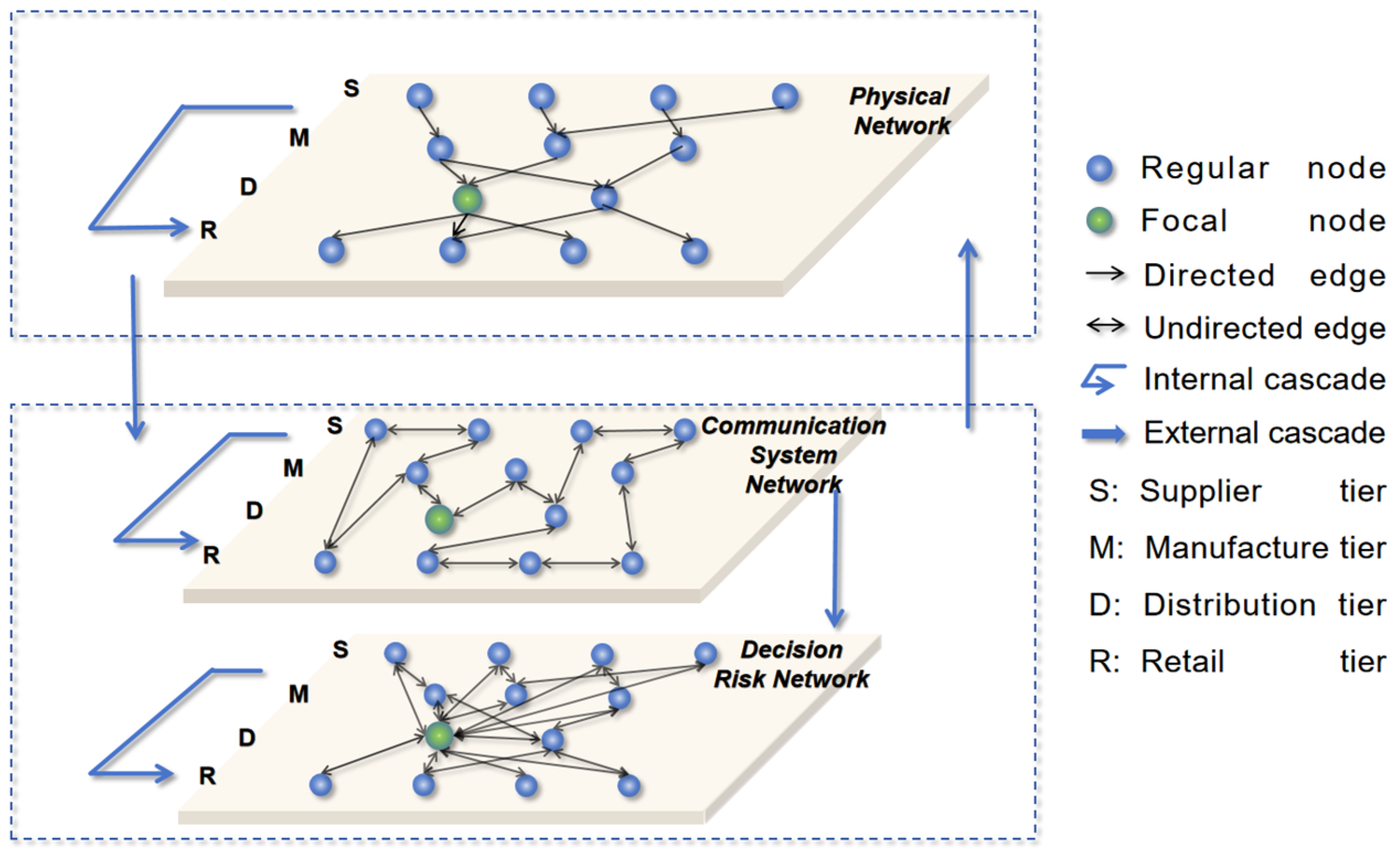
Figure 1. Coupled supply chain multi-tier network cascading failure model diagram.
Systems 13 00729 g001
Figure 2. Simplified schematic diagram of multi-load flow in Physical Network.
Systems 13 00729 g002
Figure 3. Communication System Network weight adjustment mechanism.
Systems 13 00729 g003
Figure 4. Illustration of the interactions among multi-layer coupled networks.
Systems 13 00729 g004
Figure 5. Results of RB analysis for the failure of a single Physical Network node (including both focal and regular nodes) under Physical Network load boundary fluctuation. (a) represents a focal node; (b) represents a regular node.
Systems 13 00729 g005
Figure 6. Failure of a single node in the Communication System Network under η 2 and α 2 fluctuation scenarios and its impact on R B . (a) represents the failure of a focal node; (b) represents the failure of a regular node.
Systems 13 00729 g006
Figure 7. Impact of single Decision Risk Network node failure on R B and under η 3 and α 3 fluctuation conditions. (a) Focal node failure under centralized conditions; (b) ordinary node failure under centralized conditions; (c) focal node failure under decentralized conditions; (d) ordinary node failure under decentralized conditions.
Systems 13 00729 g007aSystems 13 00729 g007b
Figure 8. Impact on R B under α and β fluctuation scenarios when a single node in the Communication System Network or Decision Risk Network fails. (a) Failure of a focal node in the Communication System Network; (b) failure of a regular node in the Communication System Network; (c) failure of a focal node in the Decision Risk Network; (d) failure of a regular node in the Decision Risk Network.
Systems 13 00729 g008
Figure 9. Impact of Physical Network node failure and operational efficiency drop in Physical Network nodes on R B under α and β perturbation scenarios. (a) Under centralized control, when a focal node fails, the operational efficiency of ordinary nodes drops to 70%; (b) under centralized control, when an ordinary node fails, the operational efficiency of other ordinary nodes drops to 70%; (c) under decentralized control, when a focal node fails, the operational efficiency of ordinary nodes drops to 70%; (d) under decentralized control, when an ordinary node fails, the operational efficiency of other ordinary nodes drops to 70%.
Systems 13 00729 g009
Figure 10. The effect of β on R B under α , β perturbations when the demand reduction level ( D R L ) for all retail tier nodes in the Physical Network is set to 60%, 50%, 40%, 30%, and 20%.
Systems 13 00729 g010
Figure 11. The effect of α and β perturbations on R B when the actual delivery load of all retail tier nodes in the Physical Network is increased to 125%, 150%, 175%, and 200%. (a) Actual delivery load increases to 125%; (b) actual delivery load increases to 150%; (c) actual delivery load increases to 175%; (d) actual delivery load increases to 200%.
Systems 13 00729 g011aSystems 13 00729 g011b
Table 1. Comparison of domestic and international related studies.
Related StudyMulti-layer Coupled NetworkLoad Recovery StrategyMulti-Load Failure ModeMulti-Attack ScenarioCentralized Supply Chain Research Focus
Liu [7]×××/
Wang [8]×××/
Huang [11]××/
Mu [12]×/
Ye [25]××××Relationship with JIT
Giannoccaro [26]××××The importance of decision-maker
This studyCascading failure
Disclaimer/Publisher’s Note: The statements, opinions and data contained in all publications are solely those of the individual author(s) and contributor(s) and not of MDPI and/or the editor(s). MDPI and/or the editor(s) disclaim responsibility for any injury to people or property resulting from any ideas, methods, instructions or products referred to in the content.