A Systematic Study on Embodied Carbon Emissions in the Materialization Phase of Residential Buildings: Indicator Assessment Based on Life Cycle Analysis and STIRPAT Modeling

Abstract

Against the backdrop of intensifying global climate change and advancing the goal of the “dual-carbon” strategy, the built environment is being viewed as a complex socio-technical system in which technological, economic, demographic and institutional subsystems are coupled and evolving at different scales. As a core node in this system, residential buildings not only carry infrastructural functions, but are also deeply embedded in energy flows, material cycles and behavioural structures, which have a significant impact on carbon emissions. Given the high volume of residential buildings in China and the significant differences between urban and rural construction, there is an urgent need to systematically identify and analyse the implicit carbon emissions during the materialisation phase. In this paper, from the perspective of systems engineering, we selected 30 urban and rural residential buildings in provinces and cities from 2005 to 2020 as the research objects, adopted the life cycle assessment (LCA) method to account for the implied carbon emissions in the materialisation stage, and systematically identified the driving factors of carbon emissions based on the Stochastic Impacts by Regression on Population, Affluence and Technology (STIRPAT) model. From this study, we made the following conclusions: (1) the total carbon emissions of residential buildings in urban and rural areas in China continue to rise during the materialisation stage, showing a spatial pattern of “high in the south-east and low in the north-west”, with a significant trend of structural transformation in urban and rural areas and with steel–concrete structures dominating in towns and cities, and bricks and steel being used in rural areas. (2) Resident population and disposable income are generally positive driving factors, while the influence of industrial structure and energy intensity is heterogeneous between urban and rural areas. For overall residential buildings, every 1% increase in resident population and income will lead to a 1.055% and 0.73% increase in carbon emissions, respectively. The study shows that life-cycle-oriented carbon accounting and the identification of multidimensional driving mechanisms are of great policy value in developing urban–rural differentiated emission reduction paths and enhancing the effectiveness of carbon management in the building sector.

1. Introduction

As the global climate change situation becomes increasingly serious, reducing carbon emissions has become a strategic issue for the whole world [1,2]. Global carbon emissions from the building sector account for about 33 per cent of total greenhouse gas emissions, with CO₂ dominating; at the same time, energy consumption in the building sector exceeds 40 per cent of total global energy consumption [3]. Against this background, China, as one of the world’s largest carbon emitters, has actively responded to international emission reduction initiatives, put forward the goals of “carbon peaking” and “carbon neutrality”, and issued policy documents including the 14th Five-Year Plan, the Action Programme for Carbon Peaking by 2030, and the Implementation Programme for Carbon Peaking in Urban and Rural Construction (2023). It has also issued policy documents including the “14th Five-Year Plan”, the “Peak Carbon Action Programme by 2030” and the “Peak Carbon Implementation Programme for Urban and Rural Construction (2023)”, stressing the importance of green and low-carbon development and energy saving and emission reduction in the urban and rural construction sectors.

Residential buildings occupy an important position in building carbon emissions. Globally, the building sector accounts for approximately 39% of energy-related CO₂ emissions, of which operational carbon constitutes about 28% and embodied carbon about 11%, with the latter having become a critical focus for whole-life-cycle emission reductions [4]. In China, embodied carbon emissions from the building industry exhibited a marked upward trend between 2005 and 2020; in 2020, for instance, embodied carbon emissions reached approximately 2.28 GtCO₂—around one quarter of the nation’s energy-related emissions for that year—with upstream material production as the dominant contributor [5,6]. These facts indicate that, beyond the operational phase, the materialization stage (encompassing pre- and post-construction materials and building processes) is likewise a key area for achieving the “dual-carbon” targets and should be advanced in coordination with macro-level factors such as urbanization and industrial structure adjustment. The rapid expansion of residential construction further highlights the urgency of carbon emission research in the residential building sector. In the life cycle of residential construction, the implied carbon emissions in the physical phase (i.e., building material production, transport and construction phases) are particularly important [7]. Although the physicalisation phase accounts for a relatively low proportion of the total carbon emissions of the whole life cycle of a building (about 20%), it has a short construction cycle and high emission intensity, accounting for about 14–21% of the carbon emissions of the whole process of construction, with obvious short-term environmental impacts [8,9]. In addition, with the updating of construction technology and materials in embodied carbon emissions in recent years, the structure of urban and rural dwellings has changed markedly, with urban dwellings gradually being dominated by reinforced concrete structures, while rural dwellings have diversified and coexisted (e.g., brick–concrete, steel–concrete, and traditional timber structures) [10]. However, the systematic differences in implied carbon emissions at the stage of residential building construction between urban and rural areas and the factors influencing them have not been sufficiently explored in existing studies, and the spatial heterogeneity between provinces and cities has not been sufficiently paid attention to. Therefore, it is necessary to carry out a systematic study on implied carbon emissions at the stage of residential building construction at the urban–rural, provincial and municipal scales.

In order to effectively support the realisation of China’s “dual-carbon” strategy, this paper focuses on the implied carbon emissions of urban and rural residential buildings at the stage of building construction, and proposes targeted emission reduction measures by clarifying the current status of urban and rural residential buildings’ carbon emissions in each province and city, and by exploring the key driving factors and their spatial differences. The significance of this study is as follows: Firstly, it provides a more detailed database for the carbon emission accounting of urban and rural residential buildings at the stage of building construction in various provinces and cities in China. Although some studies have been conducted on the accounting of carbon emissions during the building construction stage, most of them are limited to a single building or a specific type of building, and few studies have analysed the implied carbon emissions of residential buildings in each province and city from the urban–rural differences and spatial dimensions. Secondly, the key factors affecting carbon emissions from residential buildings should be explored in depth, and a practical policy basis should be provided. Although existing studies generally agree that population, economic income, energy intensity and industrial structure are important drivers of carbon emissions, systematic exploration of urban–rural and inter-provincial differences is still limited. By identifying and analysing the impacts of these factors at different spatial scales and in different urban and rural contexts, this paper will help local governments to formulate more precise energy-saving and emission reduction policies.

Based on the above research background and significance, this paper specifically seeks to answer the following two research questions: (1) What is the current status of implied carbon emissions at the stage of urban/rural residential building construction and how do they differ in China’s provinces and cities in 2005 and 2020? (2) What are the key factors affecting the implied carbon emissions of urban and rural residential building construction stages, and what are the spatial differences in the performance of these factors?

Overall, numerous studies have confirmed that population size, income level, industrial structure, and energy intensity are closely associated with building-related carbon emissions, including embodied carbon. National- and provincial-scale research over the past five years has further revealed the spatial correlations and spillover effects of embodied carbon emissions, and quantified the differentiated impacts of various drivers at both local and neighboring scales; however, fine-grained identification of urban–rural disparities remains insufficient [11,12]. Accordingly, this study conducts embodied carbon accounting and driver identification from a dual provincial–urban–rural perspective, thereby addressing existing gaps in the literature concerning spatial heterogeneity and urban–rural differences. This paper firstly applies the life cycle assessment (LCA) methodology to account for the implied carbon emissions of urban and rural residential building construction phases in 2005 and 2020 in Chinese provinces and cities, and then analyses the key factors affecting the implied carbon emissions of urban and rural residential building construction phases through the extended the Stochastic Impacts by Regression on Population, Affluence and Technology (STIRPAT). A panel data fixed-effects model and a systematic GMM model are used to improve the robustness and accuracy of the study. Compared with existing studies, the innovative and expected contributions of this paper are reflected in the following aspects: (1) Focusing on urban–rural differences and spatial heterogeneity, a systematic accounting model of carbon emissions in the physical phase of residential buildings covering urban and rural areas in 30 provinces and cities is constructed to provide data support for an in-depth understanding of urban–rural differences. (2) For the first time, the extended STIRPAT model and the fixed-effects model are used to systematically explore the spatial heterogeneity of carbon emission drivers in urban and rural residential buildings, which makes up for the lack of spatial and urban-rural differentiation analyses in the current literature. (3) Based on the findings of the study, more targeted and operable emission reduction measures and policy recommendations are proposed to promote more effective energy saving and emission reduction actions in urban and rural residential buildings.

The specific arrangement of this paper is as follows: Part I is the introduction; Part II is the current status of domestic and international research and literature review; Part III describes the theoretical foundation and methodology, and explains in detail the applicability of the LCA Method and the STIRPAT model; Part IV carries out the accounting of implied carbon emissions at the stage of residential building construction; Part V carries out empirical analyses of the influencing factors; and Part VI puts forward the policy recommendations and future research directions. The sixth part proposes policy recommendations and future research directions.

2. Literature Review

2.1. Methods and Targets for Carbon Emission Accounting in the Building Fabrication Phase

The physical phase is an important part of the whole life cycle of a building, which mainly includes the production of building materials and the construction phase. Although the physical phase accounts for about 20% of the full cycle carbon emissions, its construction cycle is concentrated, only 2–3 years, which is shorter than that of the use and recycling phase (about 70 years); and in the process of China’s rapid urbanisation, the construction scale is huge, and the intensity of short-term carbon emissions is high, so it can be seen that the importance of researching the carbon emissions of the physical phase is self-evident. Existing domestic and international research on carbon emissions in the physical phase of construction mainly focuses on the following aspects: accounting methods for building carbon emissions, carbon emissions from building materials, and carbon emission characteristics of buildings of different structures.

2.1.1. Methodologies for Accounting for Carbon Emissions from Buildings

Carbon emissions accounting is the primary task before formulating carbon reduction policies. Domestic and international scholars have conducted extensive research on building carbon emissions accounting, primarily employing methods such as LCA, input-output analysis (IO), the IPCC inventory method, and direct measurement methods. Most studies have focused on calculating carbon emissions from buildings using LCA for specific stages or the entire life cycle of different objects, with the research subjects primarily being single buildings or single building types. Buildings can be categorised by their use into commercial buildings, residential buildings, public buildings, etc., with distinct carbon emission characteristics across different types. Dong Kairong (2018) noted that the entire life cycle of large-scale complexes includes four stages: building material production, construction, use, and demolition [13]. Taking residential buildings as an example, significant carbon emissions and energy consumption occur during the stages of building material production, construction, operation, and disposal [3]. Studies at the single-building level can more accurately consider the building’s own structure and material usage. For example, Feng Guohui et al. (2022) [14] used LCA to disaggregate and calculate carbon emissions across all stages of the life cycle of a near-zero energy building in Shenyang. The results showed that the cumulative carbon emissions from material production and transportation and construction accounted for 52.6% of total carbon emissions, exceeding half of the total, indicating that these two stages are critical in emission reduction efforts [14]. In contrast, macro-level studies on carbon emissions across the entire building industry value chain are limited, primarily relying on the input–output method to estimate carbon emissions in the construction sector. Jonas et al. (2007) assessed carbon emissions in Sweden’s construction sector using a top-down input–output approach, finding that indirect carbon emissions—those generated by other sectors (such as transportation)—constituted the primary component of the sector’s carbon emissions [15]. Liu Jing (2018) studied the carbon emissions of the entire building industry chain from a carbon footprint perspective, further confirming that indirect carbon emissions account for the vast majority (98–99%) of building carbon emissions [16]. Complementing these approaches, Wiik (2025) compiled 186 Norwegian building LCA case studies to develop harmonised whole-life carbon benchmark values by typology and performance level, providing reference ranges that support cross-project comparisons and policy limit-setting [17].

In terms of specific calculation methods, many scholars have conducted comparative studies on various methods and achieved results. Liu Mingda et al. (2014) compared the advantages, disadvantages, and applicability of the emission factor method, mass balance method, and measurement method [18]. The emission factor method originates from the IPCC methodology, and its conclusions are authoritative and applicable to macro, meso, and micro levels; however, it is difficult to adapt to complex and dynamic emission systems. The mass balance method is suitable for macro and meso-level analysis and can adapt to system changes; however, its methodology and operational details are not yet standardized, and research conclusions vary significantly. The measurement method yields precise results but faces challenges in data acquisition and is limited to small-scale micro-level calculations. Shen Liyin et al. (2015) summarised the system boundaries and data characteristics of the life cycle process method and the input–output method: the input–output method is based on energy balance tables and yields relatively coarse results; the process method provides precise data but has unclear system boundaries and suffers from truncation errors, which affect the accuracy of results [19]. Huang Zhi-jia et al. (2014) analysed carbon emissions from six stages of building material production, transportation, construction, decoration, operation, and demolition and recycling, proposing a method of multiplying ‘activity factors × emission coefficients’ to achieve a more comprehensive carbon emission calculation for the building life cycle [20]. Additionally, beyond static carbon accounting, Wu et al. (2017) conducted dynamic life cycle carbon emission calculations for green buildings and non-green buildings [21]. Extending the methodological discussion from accounting to implementation, Moghayedi and Awuzie (2025) propose a practical framework for delivering low-income net-zero energy housing in developing countries—emphasising the integration of technical design with financing, governance and stakeholder coordination—which complements LCA/IO choices by embedding whole-life carbon monitoring into delivery and operation [22].

2.1.2. Building Carbon Accounting Objects

Researchers have also focused on the carbon footprint of building materials and the differences in carbon emissions among various types of building materials. Carbon emissions during the production stage account for the highest proportion of total carbon emissions across the entire life cycle of building materials, exceeding 70% in the four stages of raw material acquisition, raw material transportation, building material production, and building material transportation [23]. Even when upstream energy production stages are included in the evaluation scope, the results still indicate that the production stage accounts for the largest proportion of carbon emissions [24]. Regarding the differences in carbon emissions among various building materials, scholars have studied the carbon emissions of cement, concrete, wood, aluminium, insulation materials, and other building materials during the construction stage of residential buildings. The results consistently show that the combined carbon emissions of major building materials such as steel, wood, and cement account for over 80%, with steel having the largest proportion [25,26,27]. This finding aligns with national-level analyses indicating that material production contributes over 80% of total building-sector carbon emissions [6]. Differences in building structural systems influence carbon emissions by affecting building material usage and construction methods. Studies indicate that traditional wooden structures have lower energy consumption and carbon emissions over their entire life cycle compared to light steel structures and reinforced concrete structures [28,29]; green buildings reduce carbon emissions by approximately 20% compared to conventional buildings [30]; and building shape coefficients also significantly impact energy consumption and carbon emissions [31].

Generally speaking, the current accounting of carbon emissions in the physical phase is mostly based on LCA, combined with methods such as emission factor method, input–output method and relevant statistics. There are more micro-level studies than macro-level studies, and there are relatively few studies that account for carbon emissions of urban and rural buildings separately. Carbon emissions in the physical phase of different types of buildings show some common characteristics: carbon emissions in the production phase of building materials account for a large proportion, and carbon emissions from various types of building materials are mainly concentrated in steel, concrete, wood, cement, etc., which show an obvious inclination; different structural systems also affect the intensity of carbon emissions. Since the carbon emission in the materialisation stage is implicit carbon and does not involve the whole industrial chain, life cycle evaluation method is usually adopted in carbon accounting, and carbon emission accounting is carried out in the whole process of the materialisation stage from the production and transportation of building materials to the construction of a single type of building.

2.2. Factors Affecting Carbon Emissions from Buildings

At the macro level, academic research on the factors influencing carbon emissions from buildings mainly focuses on factor decomposition analyses and corresponding emission reduction measures. Commonly used methods include Kaya’s Constant Equation, Logarithmic Mean Dee’s Index Decomposition (LMDI), STIRPAT model, IPAT model, and Granger causality test, etc., and the examination of demographic, economic, energy structure, industrial structure and other factors is more concentrated. Due to the different research objects and methods, there are some differences in the conclusions drawn by the studies. In addition, regarding embodied carbon, scholars have begun to pay attention to the impact of institutional and financial factors other than traditional factors on building carbon emissions. On the one hand, some studies have found that the degree of decentralisation of environmental governance in China has a significant impact on carbon emissions, and that excessive environmental decentralisation may exacerbate carbon emissions when a certain threshold is exceeded [32]. On the other hand, financial innovations such as digital inclusive finance have been shown to promote inclusive green development at the city level, which indirectly contributes to carbon emission reductions [33]. Financial support policies targeting rural areas have likewise been shown to help reduce carbon emissions [34].

In factor modelling, we used Kaya’s constant equation to analyse the drivers of carbon emissions from residential buildings, which can be classified into four categories: energy mix, population size, economic output and energy intensity, with economic output being the main driver and energy intensity being the most significant inhibiting factor [35,36]. Based on this, we further applied the LMDI decomposition method to decompose the carbon emission changes into the pre-determined factors and found that the growth of GDP per capita and the expansion of the population size will significantly push the carbon emission increase [37]. The LMDI decomposition combined with the Tapio decoupling theory allows further exploration of the relationship between building carbon emissions and output value and the factors influencing it [14]. In addition, Yu et al. (2019) empirically analysed the relationship between overall carbon emissions and economic growth in China by combining the Tapio decoupling model with the Environmental Kuznets Curve (EKC), assessing the state of decoupling of carbon emissions at the national level as well as at the provincial level, which provides a reference to understand the relationship between carbon emissions and economic development at the macro level [38]. Zhang Xiaohou, by using the IPAT model, found that there is a high correlation between building energy consumption and the completed area at the end of the year and per capita living energy use [39]. From the perspective of the whole life cycle of buildings, analysis using the STIRPAT model shows that the population urbanisation rate, per capita income and per capita living space are important factors influencing carbon emissions from buildings in Beijing [40]. Further research based on the STIRPAT model found that building carbon emissions are positively correlated with drivers such as per capita living space, building footprint, household consumption level, and carbon intensity per unit of building area in different climate zones, but the extent of the correlation varies depending on the climatic conditions [41]. The results show that residential building area and resident population have the greatest influence on carbon emissions. Liu Xinghua et al. analysed the factors affecting carbon emissions from residential buildings in Guangzhou based on the STIRPAT model and combined with ridge regression, and the results showed that residential floor area and resident population had the greatest impact on carbon emissions [42]. In addition, some scholars studied the relationship between the gross output value of the construction industry and carbon emissions with the help of the Granger causality test. In addition, some scholars have studied the relationship between the gross output value of the construction industry and carbon emissions with the help of the Granger causality test, and have found that the gross output value of the construction industry has a significant contribution to carbon emissions, and vice versa [43].

Aiming at the main influencing factors of carbon emissions from buildings at different stages, some studies proposed corresponding emission reduction countermeasures accordingly. Qi Shenjun et al. focus on the fact that the use stage of buildings and the production stage of building materials account for a high proportion of carbon emissions, and propose that attention should be paid to the application of new emission reduction technologies in the process of architectural design, and that the service life of buildings should be reasonably determined [44]. Lai et al. (2017) analysed the drivers and influencing factors of low-carbon development in the construction sector, pointing out that there should not be an over-reliance on a single driver, as the strength of a single factor in pulling emission reductions is more limited in the long term [45]. Ma et al. constructed an optimisation model to measure carbon emissions and intensity after disaggregating carbon emissions, and found that the rapid development of China’s economy and urbanisation is not conducive to carbon emission reduction, and that reducing energy consumption and optimising the industrial structure are important measures to promote low-carbon green development [46]. There are also studies that use the system dynamics (SD) approach to comprehensively assess the mechanisms of the influencing factors and construct simulation models, which are conducive to considering the interrelationships among the components from a holistic perspective of the system [16]. Overall, there is a lack of a standardised and nationally appropriate evaluation system for carbon reduction policies in buildings, and there are fewer empirical studies with large samples, so the emission reduction paths and their effects still need to be further verified.

In general, most of the existing studies on the influencing factors of carbon emissions from buildings focus on factors such as population, economy, energy structure, industrial structure, etc. A variety of factor decomposition methods are applied, especially LMDI decomposition, STIRPAT model, etc., and corresponding emission reduction measures are proposed in combination with the results of the analyses. In terms of research objects, most of the studies on residential buildings focus on the overall carbon emissions or the use phase, and there are relatively few studies on the influencing factors of the implied carbon emissions in the materialisation phase. In terms of research methodology, compared with the LMDI decomposition based on Kaya’s constant equation and the IPAT model, the STIRPAT model is more flexible in its use, can incorporate more complex and diverse factors, and is conducive to revealing the drivers of carbon emissions, and is therefore more suitable for the analysis of such issues.

2.3. Literature Evaluation

The above summarises the current status of domestic and international research on building carbon emission accounting and its influencing factors. In terms of carbon emission accounting at the stage of building construction, a large number of studies have used LCA, IPCC inventory method, input–output method and so on to account for building carbon emissions, but there are more studies at the micro level than at the macro level, and there are still fewer studies that have separately accounted for urban and rural residential buildings in various provinces and cities of China and made comparisons of spatial differences. In terms of influencing factors, most of the studies have used models such as Kaya’s Constant Equation, LMDI, STIRPAT, IPAT, and Granger to explore the driving factors of carbon emissions from buildings, focusing on the impacts of population, economic development, urbanisation, and technological advancement, etc. Over the past five years, research on embodied carbon in residential and building sectors has made substantial advances in terms of accounting boundaries, data tools, and benchmark development. National-scale series covering 2005–2020 have delineated the temporal trajectories, sectoral composition, and the “material-dominated” structural characteristics of embodied carbon emissions in the building industry [5]. At the methodological and tool level, systematic reviews have compared LCA databases and assessment tools, and synthesized empirical evidence on emission-reduction strategies such as structural system selection, material substitution, resilient design, and structural retrofitting [47]. For residential buildings, methods and empirical studies for establishing embodied-carbon benchmarks and reference ranges are emerging [48]. At the urban and building-stock level, integrated frameworks combining high-resolution building-stock data with urban-scale simulations have been developed to quantify the impact of city-level policies on embodied carbon emissions [49]. Meanwhile, spatial correlation and spillover effects of embodied carbon at national and regional scales have been further substantiated, yet more fine-grained evidence is still needed to support analyses of urban–rural heterogeneity [11,12]. Many existing research objects belong to the micro level, and different methods sometimes lead to divergent conclusions. In addition, the exploration of the influencing factors of implied carbon emissions in the construction (materialisation) stage is clearly insufficient. For example, a recent national-scale study reported that China’s building embodied carbon emissions reached 2.28 billion tCO₂ in 2020 (about 25% of national emissions) [5]. However, many of the existing research objects belong to the micro level, and there are some differences in the conclusions reached by different methods. In addition, the exploration of the influencing factors of implied carbon emissions in the physicalisation stage is obviously insufficient. Overall, there is a gap in research that distinguishes between carbon emissions at the physicalisation stage of urban and rural residential buildings and analyses their drivers at the macro level.

This paper aims to address these gaps by, on the one hand, taking into account the differences between urban and rural buildings in different regions of China, accounting for the implied carbon emissions at the residential building construction stage by urban and rural areas and comparing the regional differences; and, on the other hand, analysing the drivers of carbon emissions at the physical stage by applying the STIRPAT model, which is a more inclusive model. By combining macro-statistical analysis with life-cycle carbon accounting, the research in this paper will help to make up for the shortcomings of the existing literature in accounting for carbon emissions and analysing the influencing factors in the physical building phase at the macro level, and thus provide a new empirical basis and research perspective for the formulation of targeted building carbon reduction policies.

3. Research Design

3.1. Theoretical Foundation

3.1.1. Life Cycle Theory Foundation

Life cycle theory emphasises the assessment of the environmental impact of a product or system from cradle to grave, i.e., a comprehensive accounting of the impacts of the entire process of raw material acquisition, production and manufacturing, use and operation, and disposal at the end of life. This idea first sprouted from the exploration of the environmental impact of packaging containers by the Midwest Research Institute in the 1960s, and has since been gradually developed into the LCA methodology. In the mid-1990s, LCA began to be applied to the field of construction, realising the expansion of environmental impact assessment from a single product to a complex building system [50]. The International Organisation for Standardisation (ISO) issued a series of LCA standards in 1997, which clearly define the principles and framework of LCA, including four phases: objective and scope definition, life cycle inventory analysis, impact assessment and result analysis. In the construction field, LCA can be classified into “cradle to grave”, “cradle to site” and “cradle to end of construction” according to the different scopes of study [51]. “From cradle to grave” is the complete life cycle, while “from cradle to end of construction” covers the physical stages of building material production, transport and construction. This study focuses on the carbon emissions of urban and rural residential buildings during the physicalisation phase, which is the upstream process from raw material production to the completion of the building, as part of the life cycle of residential buildings. Adopting the life cycle theory as the basis of the study ensures that the implied carbon emissions in the process of residential construction are fully included in the scope of accounting, which theoretically meets the requirements of the whole-process control of carbon emissions in the construction field.

3.1.2. Theoretical Basis of the STIRPAT Model

The STIRPAT model is a classic theoretical model for analysing the impacts of human activities in environmental sciences, the core of which is derived from the IPAT model, which was proposed by Ehrlich and Holdren in the 1970s to express the multiplicative relationship between the environmental impact (Impact, I) and the population (Population, P), the affluence (Affluence, A) and the technology level (Technology, T) in a simple constant equation. The IPAT model describes quantitatively the impact of a single factor change on environmental pressures in a multiplicative form, but its applicability is limited by the assumption of linear year-on-year changes in the factors, which does not reflect the non-linear effects of multiple factors and statistical significance [52]. To overcome the shortcomings of the IPAT model, York et al. proposed the STIRPAT stochastic regression model in 1993, which extends and improves the IPAT formulation [53]. STIRPAT retains the framework of population-affluence-technology impacts on the environment, but introduces exponential power parameters to be estimated and random perturbation terms, transforming the model from a constant equation to a regressively estimable nonlinear form. Its general form is expressed as follows.

$$I=a\times P^b\times A^c\times T^d\times e$$

(1)

a is the model coefficient, the constant term; b, c, and d are the elasticity coefficients corresponding to the population factor (P), the wealth factor (A), and the technology factor (T), respectively; and e is the error term. In order to facilitate data processing and analysis, both sides of the equation are logarithmised and the converted expression is as follows:

$$lnI=a+blnP+clnA+dlnT+e$$

(2)

Compared with IPAT, the STIRPAT model has significant theoretical advantages: firstly, the elasticity coefficient reflects the non-proportional rate of change of the 1% change of each factor on the environmental impact, portraying the elasticity of the factor impact rather than a simple year-on-year relationship; secondly, the model allows for the addition of new driving factors according to the needs of the study (e.g., urbanisation rate, industrial structure, etc.), which breaks through the limitations of the IPAT’s fixed triad of factors, and has stronger expandability and applicability [53]. For this reason, the STIRPAT model has been widely used in the field of carbon emission driver analysis to explain the influence of demographic, economic, technological and other social factors on carbon emissions. In summary, the life cycle theory and STIRPAT model provide theoretical support for this paper from the emission accounting and driver analysis levels: the former ensures the scientific integrity of the carbon emission accounting of the urban and rural residential construction process, and the latter provides a reliable analytical framework for exploring the influencing factors and mechanisms of carbon emission. The combination of the two fits the complexity of the research object of this paper, and lays a solid theoretical foundation for the study of carbon emission and its influencing factors in the building process of urban and rural housing.

3.2. Research Methodology and Modelling

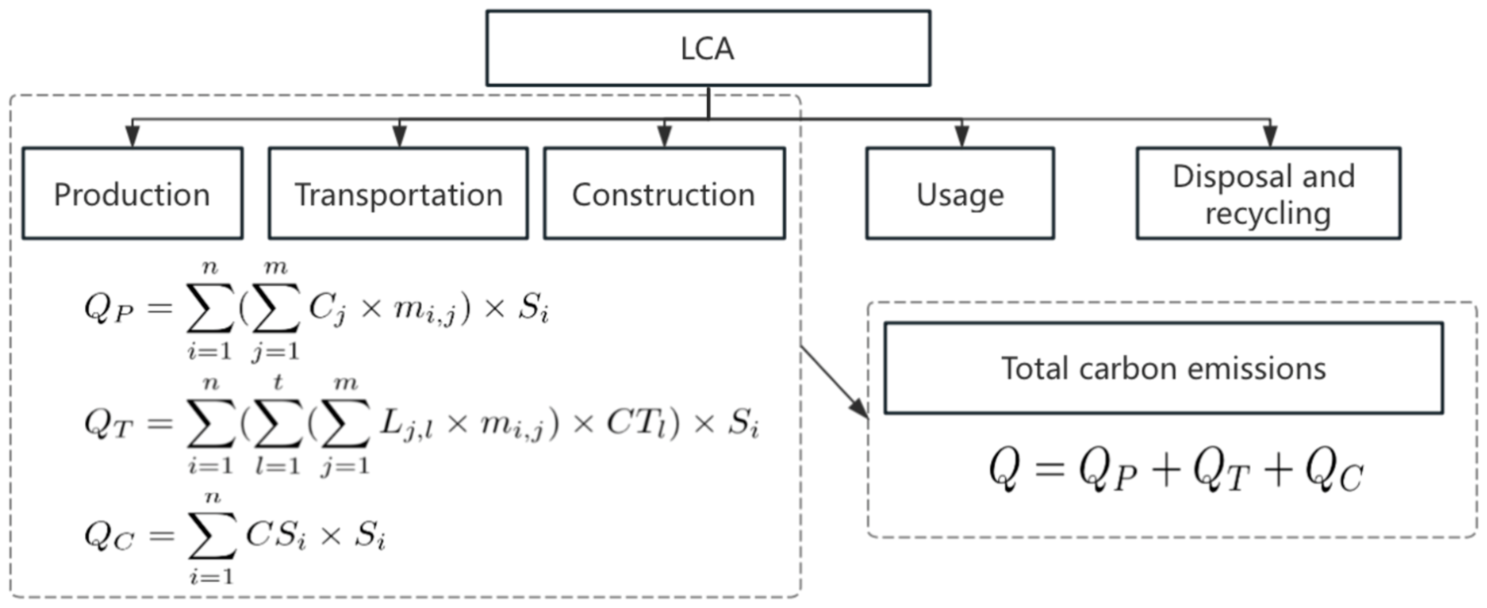
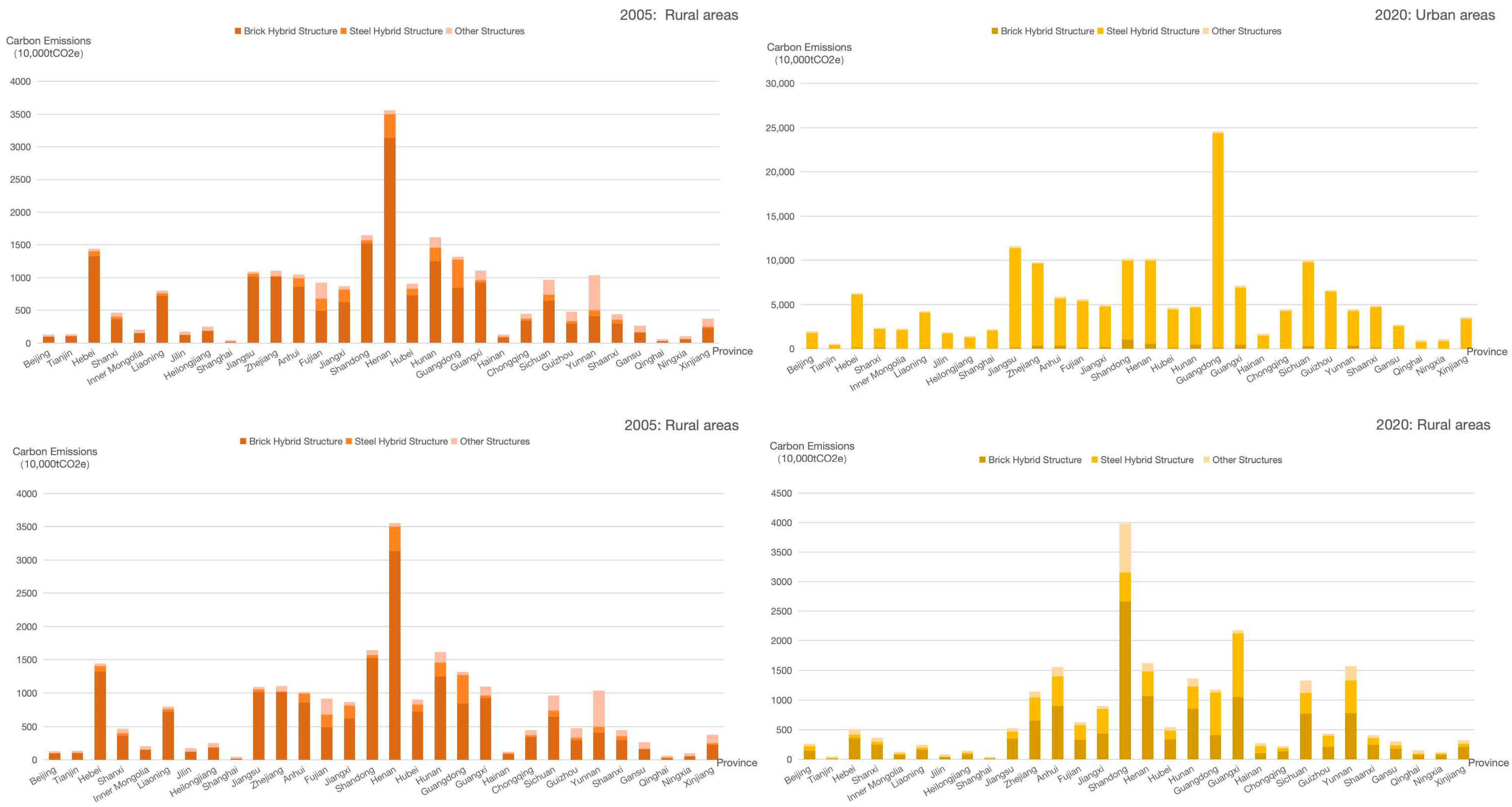
Based on the above theoretical framework, the research methodology of this paper includes two parts: carbon emission accounting and impact factor analysis, corresponding to the LCA method and the STIRPAT model regression analysis method, respectively. In terms of method selection, it is necessary to ensure both the comprehensiveness and accuracy of carbon emission measurement and the scientific and effective analysis of driving factors. In view of this, this paper adopts the process analysis idea in the LCA method in carbon emission accounting, and calculates the carbon emission of the residential building construction stage by the emission coefficient method; and adopts the STIRPAT model extension regression method in the analysis of the influencing factors, and demonstrates its applicability by comparing with other models. The specific contents of these two parts of the method are introduced separately below.

3.2.1. LCA Approach to Accounting for Carbon Emissions

System boundaries and functional units: The first step in LCA is to define the system boundaries and functional units of the study. The system boundary refers to the delineation of the scope of processes included in carbon accounting. The whole life cycle of a residential building consists of five phases: production of building materials, transport, construction, use and operation, and dismantling and recycling. This study focuses on carbon emissions from the physical phase, so the system boundary is limited to the three upstream processes of building materials production, building materials transport and construction, excluding emissions from residential use and dismantling and recycling phases. This choice of boundary is equivalent to the “cradle to construction end” in the LCA category, which covers all the carbon-containing activities that occur before the house is put into use. Within this scope, the carbon emissions from the production of building materials mainly come from the energy consumption and process emissions of raw material extraction, processing and manufacturing of building materials; the emissions from the transport of building materials come from the fuel consumption of transport vehicles and losses in the transport process; and the emissions from the construction process come from the operation of construction machinery and equipment and the energy consumption at the construction site. In terms of functional units, in order to facilitate the horizontal comparison of carbon emissions under different scenarios, it is necessary to select a unified reference benchmark. In view of the large differences in the scale of residential buildings in different regions and the lack of comparability in directly comparing the total carbon emissions, this paper adopts the carbon dioxide equivalent emissions per unit of building area (kg CO₂e/m²) as the functional unit. This functional unit is commonly used in the study of building carbon emissions, which can effectively improve the comparability of carbon emission indicators of different regions and different types of buildings.

Accounting method and selection of emission coefficients: This paper adopts the process analysis method of life cycle assessment to account for carbon emissions in the materialisation phase of urban and rural housing. Specifically, the emission factor method is used to establish a carbon emission calculation model, i.e., multiplying the activity level data with the corresponding carbon emission factor and adding them up. This method is equivalent to combining the “activity factor” and “emission factor” of construction activities, which can be detailed to different materials and processes, and has a higher accuracy for carbon accounting of complex systems. In contrast, macro-accounting methods such as the input–output method have relatively rough results because they are based on input–output tables or energy balance tables, while the traditional process method uses fine data but the system boundary is not easy to be clarified, and it is prone to truncation errors, which affects the accuracy of the results. Therefore, this paper draws on the research ideas of Huang Zhijia et al. (2014) [20] to improve the life cycle carbon accounting of residential buildings by multiplying the activity level by the emission factor. The accounting model is constructed according to the three sub-processes of the materialisation stage, respectively:

At the building material production stage, carbon emissions are calculated using the energy consumed in the production of various types of building materials and emission factors. The calculation formula is as follows:

$$Q_P=\sum _{i=1}^n\left(\sum _{j=1}^m{C}_j\times m_{i,j}\right)\times S_i$$

(3)

Q_P is the carbon emissions from the production process of building materials; S_i is the floor area of the ith residential structure; C_j is the carbon emission factor of the jth building material in the production process of building materials; m_i,j is the consumption of the jth building material per unit floor area of the ith residential structure.

In the building material transport stage, the transport emissions are calculated using the transport distance of building materials and the emission factor of transport means. The calculation formula is as follows:

$$Q_T=\sum _{i=1}^n\left(\sum _{l=1}^t\left(\sum _{j=1}^m{L}_{j,l}\times m_{i,j}\right)\times C{T}_l\right)\times S_i$$

(4)

Q_T is the carbon emissions from the transport of building materials; S_i is the floor area of the ith residential structure; L_j,l is the distance of the jth building material transported by the lth mode; m_i,j is the consumption of the jth building material per unit of floor area of the ith residential structure; and CT_l is the carbon emission factor of the lth mode of transport.

In the building construction stage, construction emissions are calculated using construction energy consumption and construction equipment emission factors. The calculation formula is as follows:

$$Q_C=\sum _{i=1}^{n}C{S}_i\times S_i$$

(5)

Q_C is the carbon emission of the building construction process; S_i is the floor area of the ith residential structure; CS_i is the unit carbon emission corresponding to the construction stage of the ith residential structure.

The total carbon emissions of the residential building construction stage can be obtained by adding the results of the above three parts. The calculation formula is as follows:

$$Q=Q_P+Q_T+Q_C$$

(6)

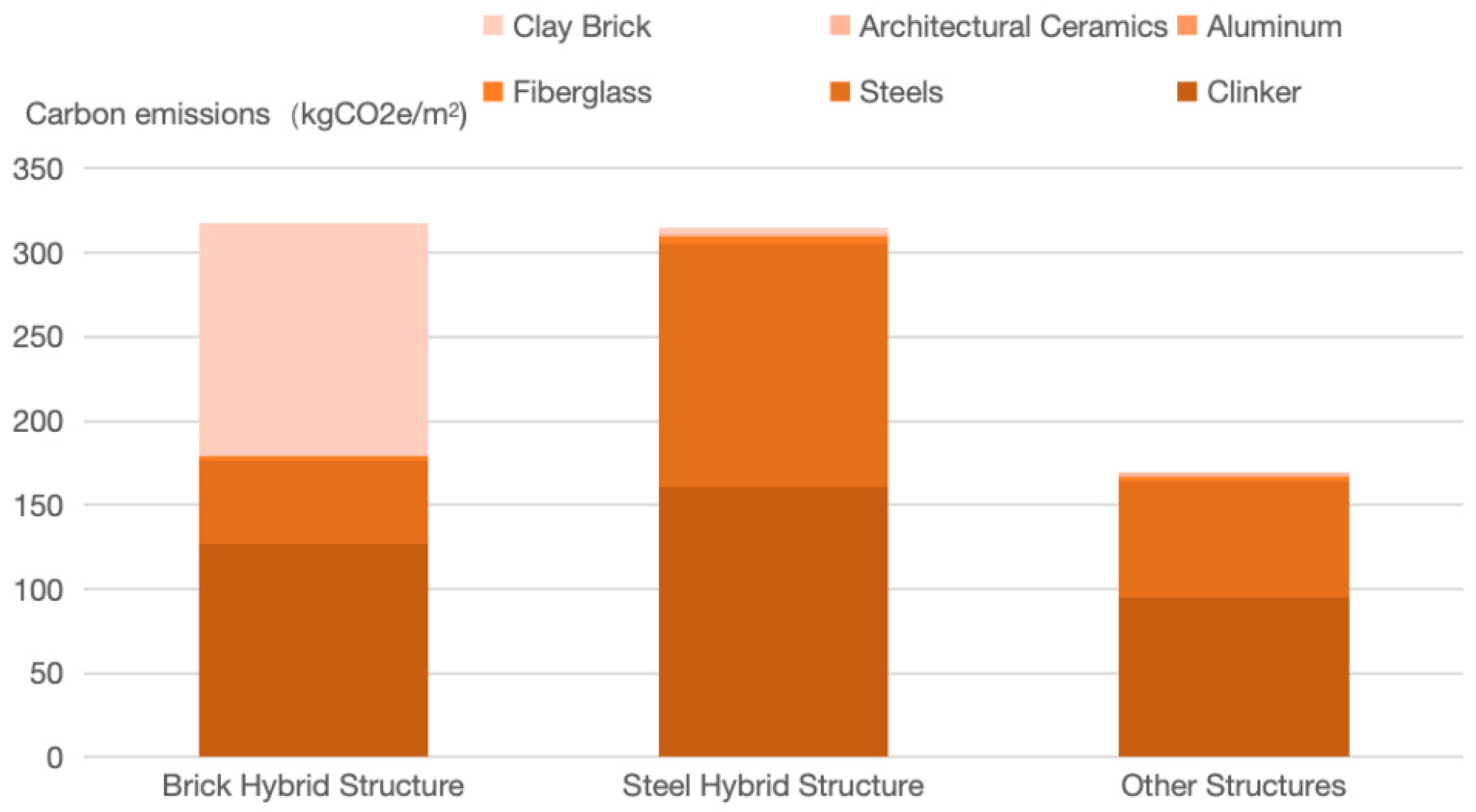
In order to improve the accuracy of accounting, this paper calculates carbon emissions separately according to the differences in residential building structure types. The study shows that the significant difference in the amount of building materials used and the level of energy consumption per unit area of residential buildings of different structural types is a key factor affecting the intensity of physical and chemical carbon emissions [28,29]. Accordingly, this paper further subdivided urban and rural dwellings into major structural types, and estimated the carbon emissions per unit area of different structural dwellings, such as reinforced concrete and brick and wood concrete, during the materialisation stage, and then combined the value with the completed area of dwellings in each province and city to obtain the total regional emissions. The calculation framework is shown in Figure 1.

In terms of data acquisition, the construction area of residential buildings by structural type is obtained from authoritative statistics such as the China Construction Industry Statistical Yearbook, and the unit consumption of building materials refers to the relevant engineering quotas and literature [28,29]. Carbon emission factors are preferred to values provided by authoritative studies and databases at home and abroad, such as the IPCC Greenhouse Gas Inventory Guidelines and the China Life Cycle Database [54]. The selection of emission coefficients follows the principle of higher rather than lower, i.e., taking the higher value when data from multiple sources are available to avoid underestimating carbon emissions. Through the above methodology and boundary setting, the comprehensiveness and comparability of carbon emission accounting in the urban and rural residential building construction stage are ensured.

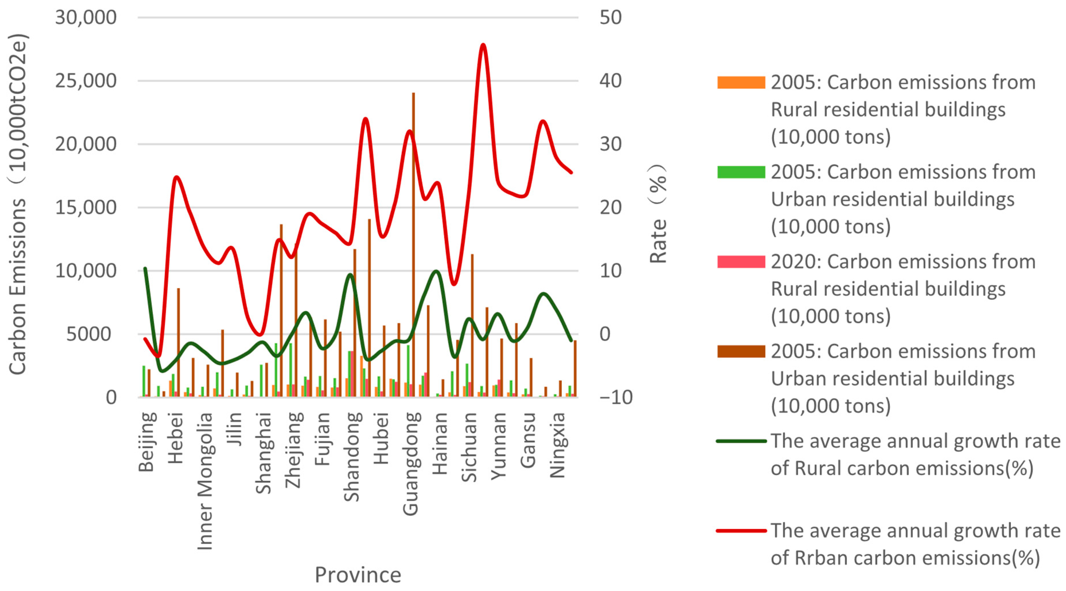
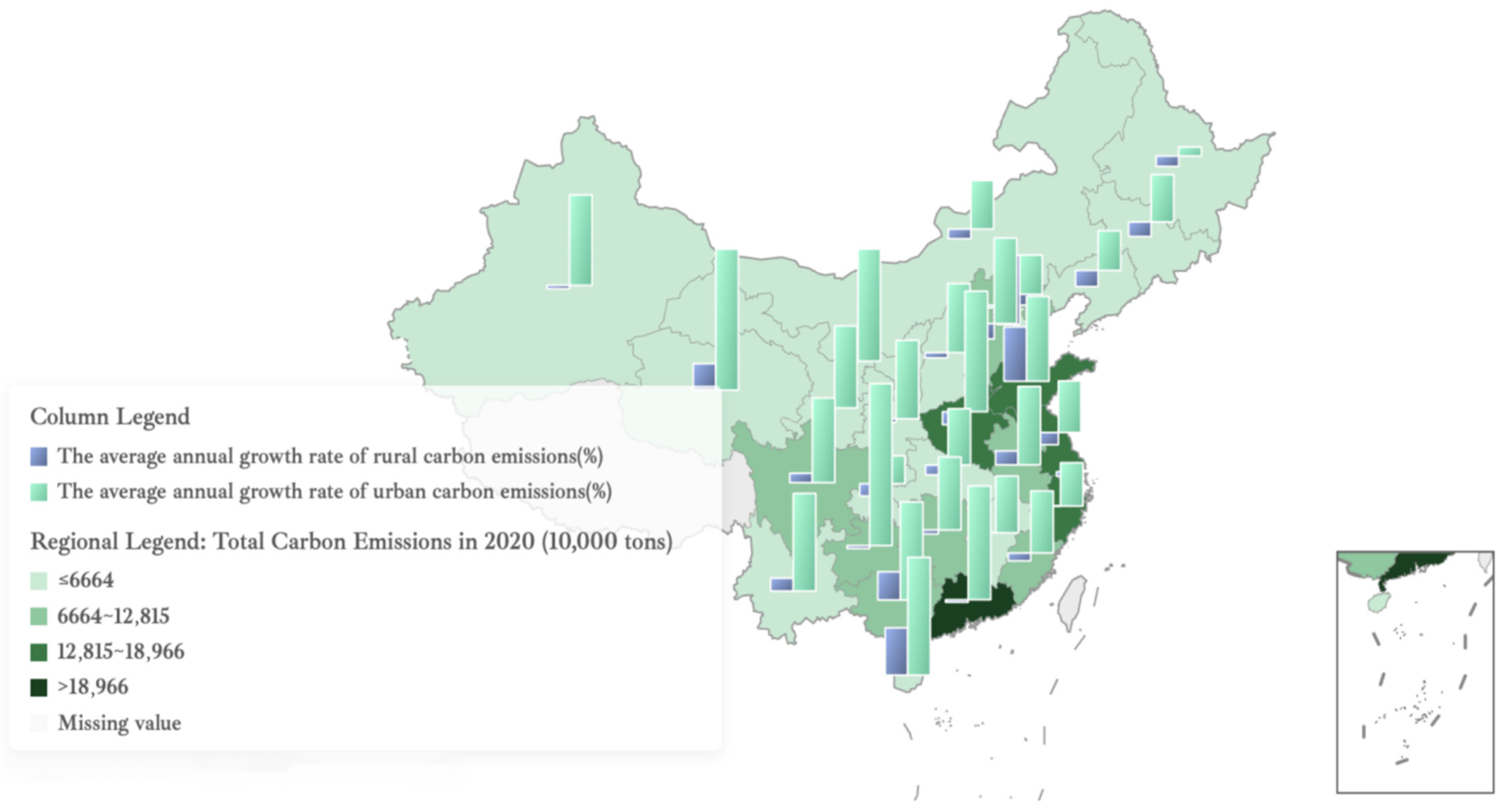
Specifically, in order to quantitatively evaluate the impact of physical carbon emissions due to the development and spatial differences between urban and rural residential buildings, this paper selects urban and rural residential buildings constructed in 2005 and 2020 in 30 provinces and cities in China (except Tibet, Hong Kong, Macao, and Taiwan), which are capable of reflecting the carbon emissions brought by the phase of residential building construction in those years. The data on the construction area of urban and rural residential buildings in each province and city are taken from the China Statistical Yearbook, China Rural Statistical Yearbook, and China Construction Industry Yearbook, and are quantified by the annual construction area of urban and rural residential buildings. The annual residential construction area includes all the buildings constructed in that year, including those that had been started or stopped before and then started again in that year, as well as the construction area of new buildings started in that year.

At present, China has not made public detailed and specific statistics on residential building structures in urban and rural areas. This paper is based on a case study on the distribution of building structures in China from 2003 to 2005 [55]. The main data from the 2005 National 1% Population Sample Survey and the relevant data from the Seventh National Population Census in 2020 were used to study China’s main residential structures and their share of the total, which, in keeping with the calibre of the Population Census, can be divided into three specific categories, namely, steel–concrete, brick–concrete and other structures. Accordingly, the proportion of urban and rural residential structures of various types in China’s provinces and cities in 2005 and 2020 was calculated, totalling 120 sets of weighted data for 30 provinces and cities, divided into urban and rural areas for each year.

Corresponding to the various types of residential structures, six types of building materials, including cement, steel, glass, aluminium, building ceramics and clay bricks, which mainly affect carbon emissions in the physical and chemical stages, were identified, and the consumption of the corresponding building materials was analysed in conjunction with the relevant literature (e.g.,

Table 1. Consumption of major building materials per unit area for different residential structures (per 100 m²).

Materials		Clinker (t)	Steels (t)	Fiberglass (t)	Aluminium (m2)	Architectural Ceramics (m2)	Clay Brick (m3)
Residential Structures	Brick Hybrid Structure	16.34	2.38	0.22	0.1	1.27	47.71
	Steel Hybrid Structure	20.71	6.95	0.34	0.18	1.95	1.24
	Other Structures	12.3	3.3	0.22	0.1	1.27	0

) [18,56].

Carbon emission factors for the production and transportation of various building materials (as shown in

Table 2. Carbon emission factors for each construction material or mode of transportation.

Materials	Carbon Emission Factors
Clinker (kgCO2e/t)	735
Steels (kgCO2e/t)	2050
Fiberglass (kgCO2e/t)	1130
Aluminium (kgCO2e/m2)	194
Architectural Ceramics (kgCO2e/m2)	19.5
Clay Brick (kgCO2e/m3)	250
Diesel Truck Transportation (kgCO2e/(t·km))	0.078

) are derived from the ‘Building Carbon Emission Calculation Standard’ issued by the Ministry of Housing and Urban-Rural Development of China and relevant literature [57,58,59], with the average values used. Carbon emissions from the production and transportation of building materials are primarily calculated from the consumption end. The default transportation distance is 500 km (in accordance with the relevant provisions of the ‘Building Carbon Emission Calculation Standard’ GB/T51366-2019) and transportation is assumed to be by diesel trucks [58]. The unit carbon emissions during the construction process of various residential building structures (as shown in

Table 3. Carbon emission factors of different residential structures during building construction stage.

Residential Structures	Brick Hybrid Structure	Steel Hybrid Structure	Other Structures
Carbon Emission (kg/m2)	24.31	45.38	14.32

) are derived from the research results of Bai Jing et al. [56,60,61], with the average values taken.

3.2.2. Comparative Analysis of the STIRPAT Model and Model Selection

Model applicability and comparative analysis: Before selecting the STIRPAT model, it is necessary to compare and evaluate it with other commonly used models. Common methods for analysing macro-level carbon emission factors include the Kaya identity and its extended LMDI decomposition method, the IPAT/STIRPAT model, and econometric regression models. The Kaya identity equation, derived from the IPAT concept, expresses carbon emissions as a constant relationship between population, economic output, energy intensity, and carbon intensity. It can be used to decompose the sources of carbon emission changes. Its improved LMDI (logarithmic mean Dice index) decomposition method fully decomposes emission increases and decreases across different time periods based on the identity equation, quantitatively assessing the contributions of various factors. Previous studies have used the Kaya/LMDI method to identify the primary drivers of building carbon emissions, such as economic growth and population expansion, which have been proven to be the main factors driving carbon emissions, while reductions in energy intensity help mitigate carbon emissions [35,36]. The advantage of this method lies in its intuitive decomposition results, where factor contributions can be summed to represent the total change in emissions. However, the Kaya identity predefines fixed decomposition factor categories, making it difficult to incorporate additional potential factors. Additionally, the decomposition analysis is a post hoc attribution approach, unable to test the statistical significance or causal relationships between factors. In contrast, the STIRPAT model, as an extension of IPAT, offers greater flexibility and applicability. First, the STIRPAT model appears in the form of a regression model, allowing the introduction of any number of independent variables, not limited to the four factors of population, GDP, energy consumption, and emissions in the Kaya identity. When the focus of the study changes (e.g., considering urbanisation rates, industrial structure, or climate factors), the model can be expanded accordingly to avoid omitting important influencing variables. Second, the STIRPAT model allows factors to influence the dependent variable through elasticity coefficients, breaking the assumption of proportional changes in factors and reflecting nonlinear effects and inconsistent returns to scale. Third, since STIRPAT is based on regression analysis, it can provide statistical measures such as significance tests and goodness-of-fit, which are more helpful for assessing the reliability of factor effects and the explanatory power of the model. These advantages have led to the widespread application of STIRPAT in the environmental field. For example, Yu et al. employed an extended STIRPAT model to incorporate climate factors into carbon emissions driver analysis, demonstrating the significant impact of temperature changes on regional carbon emissions, thereby showcasing the STIRPAT model’s applicability in complex scenario [54]. Overall, compared to methods such as the Kaya identity/LMDI decomposition, the STIRPAT model can integrate more diverse influencing factors and reveal their elasticity mechanisms, making it suitable for investigating issues such as carbon emissions from urban and rural residential buildings, which are driven by multiple socio-economic factors. For the aforementioned reasons, this study selects the STIRPAT model as the primary econometric analysis tool. During model construction and empirical analysis, we strictly adhere to econometric norms, conducting tests and controls for variable selection, data stationarity, and multicollinearity, and referencing relevant representative research results to validate the model’s rationality, ensuring the scientific validity of the conclusions. By integrating LCA results with STIRPAT regression analysis, this study comprehensively characterises the carbon emissions characteristics and underlying causes of urban and rural residential buildings across Chinese provinces and municipalities during the building phase from both quantitative and causal perspectives, providing a robust foundation for developing differentiated building emissions reduction strategies.

Model Construction and Variable Selection: After clarifying the carbon emission calculation results, this study employs the STIRPAT model to conduct a quantitative analysis of the influencing factors of carbon emissions during the materialisation phase of urban and rural residential buildings. The rationality of variable selection is determined based on existing literature findings: on the one hand, population size and economic level are widely recognised as drivers of carbon emissions [35,36]. As population urbanisation accelerates and residents’ income increases, this often leads to an expansion in residential construction scale and carbon emissions [40]. On the other hand, technical factors such as industrial structure and energy intensity influence carbon emissions per unit of output and are important sources of carbon emission differences [37]. For example, Yang et al. found through STIRPAT model analysis that Beijing’s building carbon emissions are significantly positively correlated with urbanisation rate and per capita income [40]; Cong et al.’s research indicates that building carbon emissions are positively correlated with per capita living area and household consumption levels across different climate zones [41]; Liu Xinghua et al.’s study on Guangzhou’s residential buildings also noted that residential area and population size are the drivers with the highest carbon emission elasticity coefficients [42]. Drawing on these studies, this paper adopts an extended STIRPAT framework, incorporating population size (P), per capita income (A), industrial structure (S), and energy intensity per unit of GDP (T) as the core explanatory variables, and conducts separate estimations for the overall, urban, and rural samples to identify urban–rural heterogeneity. This specification is consistent with the latest national- and provincial-scale studies on embodied carbon, which generally find that P and A exhibit robust positive elasticities, whereas the sign and magnitude of S and T vary according to regional structural characteristics and stage-specific conditions [5,11]. Moreover, the integration of process-based LCA with econometric modelling (including spatial econometrics) has been demonstrated in recent reviews and guidelines to provide a closed-loop evidence chain linking measurement, interpretation, and policy formulation [47]. It should be noted that, given the differences in structural forms and energy use between urban and rural residential buildings, this study will establish separate regression models for the overall, urban, and rural residential sectors in the analysis to compare the differences in the effects of various factors under different residential forms. Model parameters are estimated using panel data fixed-effects regression, employing parallel data from 30 provinces and municipalities in mainland China from 2005 to 2020 (time dimension: year; spatial dimension: provincial-level regions) for fitting. The reliability of the regression results is ensured through VIF value tests and significance tests on the variables [54]. The fixed effects model controls for the influence of unobservable regional characteristics across provinces and municipalities on carbon emissions, making the estimated coefficients more meaningful in practical terms. After regression, the direction and strength of the effects of each influencing factor are determined based on the magnitude and significance of the elasticity coefficients, thereby providing a basis for subsequent discussions on the mechanisms through which these factors influence carbon emissions.

Considering that the impact of the differences in economic structure among Chinese regions on carbon emissions cannot be ignored, this paper adds structural factors to the classical STIRPAT framework to construct an extended STIRPAT model. Specifically, the physical carbon emission I of urban and rural dwellings is set as the dependent variable, the number of permanent residents (P) is selected as the demographic factor, the disposable income per capita (A) as the affluence factor, the proportion of the secondary industry or the urbanisation rate, etc., as a proxy for the structural factor (S), and the energy consumption per unit of GDP (energy intensity) as a proxy for the technological progress factor (T). The exponential form of the model is as follows:

$$I=a\times P^b\times A^c\times S^d\times T^e\times u$$

(7)

I is the environmental pressure; P is a demographic factor; A is a wealth factor; S is a structural factor; and T is a technological factor. From the influencing factor identification section above, P, A, S, and T are characterised using resident population, disposable income per capita, industrial structure, and energy consumption intensity, respectively.

A is the model coefficient, the constant term; b, c, d, and e are the elasticity coefficients corresponding to the demographic, wealth, structural, and technological factors, respectively; and u is the error term.

The STIRPAT extended model is transformed into a linear equation with logarithms on each side, with the following structure:

$$lnI=a+blnP+clnA+dlnS+elnT+u$$

(8)

Among them, b, c, d and e represent the elasticity coefficients of population, affluence, structure and technology factors, respectively, reflecting the degree of elasticity influence of the changes of each factor on carbon emissions.

For the identified key factors, this paper collects the relevant data of 30 provinces and cities in 2005 and 2020 from China Statistical Yearbook and China Energy Statistical Yearbook, among which the industrial structure and energy consumption intensity are calculated based on the original data. The variables and their data sources are summarised in

Table 4. Selection of variables and data sources.

	Variant	Symbol	Source of Data
Demographic factors	Resident population (10,000)	P	China Statistical Yearbook
Wealth factors	Per capita disposable income (yuan)	A	China Statistical Yearbook
Structural factors	Industrial structure (value added of secondary industry in GDP, %)	S	China Statistical Yearbook
Technological factors	Energy consumption intensity (energy consumption/GDP, tonnes of standard coal/ten million yuan)	T	China Energy Statistics Yearbook

Note: Dependent variable I—carbon emissions at the stage of residential building construction, data from the carbon accounting results in this paper.

, and the factors are treated as disinflation at constant 2005 prices, totalling 120 sets of weights for the 30 provinces and municipalities, divided into urban and rural areas for each year.

4. Embodied Carbon Emissions Accounting in the Materialization Stage

Residential buildings play an important role in addressing the world energy crisis and climate change due to increased energy consumption and carbon emissions. Residential buildings account for about 20 per cent of full-cycle carbon emissions in the physical phase, and the importance of conducting physical phase carbon accounting is self-evident, given the large scale of the buildings and the short construction cycle, and the high intensity of carbon emissions in the physical phase. Due to the large differences in the overall residential structures and types between urban and rural areas in China, it is necessary to calculate the implied carbon emissions from the physicalisation phase of residential buildings in urban and rural areas in each province and city separately. With the development of the times, the economic construction has been vigorously developed, the construction technology has been gradually improved, and the building area of urban and rural dwellings and the structure of urban and rural dwellings have also changed greatly; therefore, this chapter will select the implied carbon emissions of urban and rural dwellings at the stage of building construction in each province and city of China in 2005 and 2020 for carbon accounting. Using LCA, the emission factor method is chosen to measure carbon emissions, i.e., the activity levels of different structural residential building phases are multiplied by the carbon emission factor, and then the total carbon emissions are summed up to obtain the total carbon emissions.

4.1. Comparative Analysis of Embodied Carbon Emissions per Unit for Different Residential Structures

Comparing the carbon emissions per unit area of different residential structures at the materialisation stage (e.g.,

Table 5. Carbon emissions per unit area at different stages of materialisation of residential structures Residential Structure.

	Brick Hybrid Structure	Steel Hybrid Structure	Other Structures
Carbon emissions (kgCO2e/m2)	342	365	182

), the carbon emissions per unit area of steel mix are the largest, followed by brick mix, while other structures (e.g., timber frame, kiln, etc.) emit less carbon, which is about 1/2 of the carbon emissions of steel mix.

Comparing the carbon emissions from the production of building materials, transport and construction of building materials at different stages of the physicalisation of the housing structure (Figure 2), overall, the production of building materials contributes the largest share of carbon emissions in all three types of housing structures.

Comparing the carbon emissions corresponding to each type of building material in different residential structures at the stages of production and transport of building materials (Figure 3), the contribution of each type of building material to carbon emissions per unit area of different residential structures varies. In brick–concrete structures, clay bricks (43.4%) account for the largest share of carbon emissions, followed by cement (39.8%); steel (15.6%) also contributes a certain proportion, while other building materials contribute less. In steel–concrete structures, cement (51.0%) and steel (46.1%) contribute equally, accounting for a majority of emissions; in other structures, cement (56.8%) and steel (41.1%) also contribute the majority of carbon emissions. Generally speaking, the carbon emissions of clay bricks and cement materials have a greater impact in brick–concrete structures, while cement and steel materials have a greater impact in the remaining two types of structures. Reducing the carbon emission factors of clay bricks, cement and steel materials through technological upgrading, or appropriately reducing the consumption of their building materials while taking into account their performance may be an effective means of lowering the carbon emissions of residential buildings.

4.2. Overall Situation Analysis

According to the life cycle evaluation method and the calculation model determined in this paper, descriptive statistical analysis of the accounting data of the implied carbon emissions of urban and rural residential buildings in the materialisation stage of residential buildings in China’s provinces and cities in 2005 and 2020 (

Table 6. Descriptive statistics of carbon emissions (million tonnes of CO₂e) at the stage of residential building fabrication.

Variable Name	Sample Size	Maximum Values	Minimum Value	Average Value	(Statistics) Standard Deviation	Median
2005: Rural	30	3288.80	16.79	704.10	668.49	581.47
2005: Urban	30	4299.89	141.08	1734.02	1166.97	1594.89
2020: Rural	30	3667.08	13.60	679.16	773.39	366.68
2020: Urban	30	24,067.35	494.32	6184.92	5108.04	5282.02

), there are obvious temporal and regional differences in the carbon emissions of the materialisation stage of residential buildings. In 2005, the maximum carbon emissions in rural areas and towns were 32,888,800 and 42.9989 million tonnes, and the minimum values were 16.79 and 1.4108 million tonnes; in 2020, the maximum and minimum values in rural areas did not change significantly, which were 3667.08 and 13.60 million tonnes, respectively, whereas the carbon emissions in towns and cities increased significantly, with the maximum value jumping to 240.6735 million tonnes, and the minimum value climbing to 4.9432 million tonnes. From the mean and median values, it is evident that carbon emissions in rural areas have steadily declined, while carbon emissions in towns have changed by nearly four times, and the gap between urban and rural carbon emissions at the stage of residential building construction has further widened.

4.3. Inter-Provincial Comparative Analysis

In order to compare the differences in carbon emissions at the stage of physicalisation of residential buildings in urban and rural areas in various provinces and cities, Figure 4 shows the implied carbon emissions and average annual growth rates of urban and rural residential buildings at the stage of physicalisation in 2005 and 2020 in various provinces and cities in China.

As can be seen from Figure 4, carbon emissions from urban residential construction in most provinces and cities show a rising trend, while rural residential construction shows a negative growth in most provinces and cities, which may be related to the increasing rate of urbanisation and the continuous development of the economy and technology, the increase in the urban population, and the rapid expansion of the scale of housing. From the value of carbon emissions, whether in 2005 or 2020, it is evident that urban carbon emissions are much greater than rural carbon emissions: on the one hand, this is related to the residential building area constructed in that year, and in most provinces and cities and the whole country, comparing urban to rural areas in that year, the scale of residential construction is larger, and the area of constructed residential buildings is larger. On the other hand, although the structure of rural dwellings has changed somewhat with the development of time, other structures (e.g., wood, bamboo, grass structures, kilns, etc.) still account for 20–30 per cent of residential construction in rural areas at the national level, and their carbon emissions are relatively low, while the proportion of other structures in cities and towns has remained below 3 per cent for a long time.

Comparing the differences among provinces and cities (Figure 5), the carbon emissions in the stage of residential building construction are affected by various factors such as socio-economic conditions, geographic location, industrial level, etc., and show spatial heterogeneity, with “more in the south-east and less in the north-west”, and “higher in populous provinces and the western region” in the growth rate of emissions. In terms of emission rate, it is “higher in populous provinces and western regions”. In terms of carbon emissions from rural residential buildings, only five provinces and cities, namely Beijing, Shandong, Guangxi, Hainan and Qinghai, have an average annual growth rate of more than 5%, and except for Beijing, the other four provinces and cities have a growth rate of more than 10% in carbon emissions from urban residential buildings, thus achieving double growth. Beijing’s urban residential building development has become more saturated, while the resident population is still increasing to expand the construction of rural residential buildings. Shandong, Guangxi and Hainan are near the sea and rapid development, economic development and population increase have maintained a high rate in recent years; Qinghai is located in inland Northwest China, and has been affected by the national “Western Development” strategy and other rapid development in recent years. Qinghai is located in the inland northwestern region and has been developing rapidly in recent years under the influence of the national “Western Development” strategy. In terms of carbon emissions from urban residential construction, all 28 provinces and cities show growth, with Tianjin being the only region to maintain a double reduction in carbon emissions from both urban and rural residential construction, with economic and industrial levels remaining relatively stable at a high level. Guizhou, as a representative of the Southwest region, shows an average annual growth rate of 45% in carbon emissions from urban residential buildings, which may be closely related to the accelerated urbanisation and strategic development of the Southwest region over the years.

Meanwhile, comparing the carbon emissions contributed by different residential structures in the materialisation stage in different provinces and cities (Figure 6), there are obvious temporal changes and heterogeneity between urban and rural areas, showing a carbon emission pattern from “urban and rural brick-concrete structures are dominant” to “steel-concrete structures are dominant in cities and towns, while brick and steel structures are also dominant in rural areas”. In 2005, except for some provinces and cities such as Guangdong, all other provinces and cities in the physical stage of carbon emissions are mainly contributed by brick–concrete residential buildings, while other structures (e.g., wood, earth, stone, kiln, etc.) in rural areas in Southwest China, such as Yunnan, Sichuan, Guizhou, etc., also contribute to a certain extent due to geographic factors and socio-economic conditions. In 2020, the physical stage of the construction of residential buildings in the countryside showed a large contribution of brick–concrete structures, with a combination of steel–concrete or other structures. In 2020, residential buildings in rural areas will also demonstrated a large contribution from brick–concrete structures and a combination of steel–concrete and other structures, while carbon emissions from urban residential buildings in the physicalisation stage were dominated by steel–concrete structures, with brick–concrete contributing a small portion of the carbon emissions. Since carbon emissions are related to the structure and size of dwellings, and technological and economic improvements may lead to a preference for more stable steel–concrete structures, an increase in the size of the population may also lead to a need for new dwellings and a shift in the structure of dwellings, as brick–concrete and other structures are generally suited to low-rise buildings, while an increase in the density of the population is more oriented towards the construction of high-rise buildings (e.g., steel–concrete structures).

In summary, the above section accounts for the implied carbon emissions in 2005 and 2020 at the stage of urban and rural residential building construction in China’s provinces and cities, and provides the results of a descriptive statistical analysis and a qualitative analysis of its influencing factors in combination with the literature and the national situation. It is demonstrated that there exists spatial and temporal heterogeneity in the carbon emissions of each province and city.

5. Analysis of Factors Influencing Embodied Carbon Emissions

In order to explore the influencing factors of implied carbon emissions at the stage of urban and rural residential building construction in each province and city, it is necessary to identify the influencing factors first, and then construct a model on the basis of which regression analyses can be carried out. On this basis, this paper considers the heterogeneity of urban and rural areas, and conducts regression analyses from the implied carbon emissions in the overall residential building construction stage, the implied carbon emissions in the urban residential building construction stage, and the implied carbon emissions in the rural residential building construction stage of each province and city, in order to put forward the corresponding emission reduction measures and policy recommendations for the reduction in the implied carbon emissions in the overall, urban and rural stages of building construction.

5.1. Overall Residential Construction in the Provinces and Municipalities

5.1.1. Descriptive Statistics

Overall, the descriptive statistics for overall residential building (

Table 7. Descriptive statistics: overall.

Variable Name	Maximum Value	Minimum Value	Average Value	(Statistics) Standard Deviation	Median
Resident population (10,000)	12,601.25	542.50	4475.84	2801.00	3904.56
Per capita disposable income (yuan)	72,232.40	3625.00	19,615.78	15,893.16	19,036.56
Industrial structure (%)	58.58	15.97	40.43	8.50	40.00
Energy intensity	4162.83	228.18	1317.55	816.49	1065.83
(tonnes of standard coal/ten million yuan)	25,118.07	197.32	4651.10	4622.30	2750.70

) show that there is a large amount of heterogeneity within the variables, and this variation mainly stems from time (across 15 years) and space (across provinces and cities). During the residential building phase, the highest carbon emissions in a single year in a single province or city can be about 250 million tonnes of CO₂e, with an average value of about 470 million tonnes of CO₂e.

5.1.2. Analysis of Regression Results

To reduce the error in the regression, the variables first need to be tested for multicollinearity. Multicollinearity means that there is a linear correlation between the independent variables, and if there is multicollinearity, the regression coefficients will have a large error [62]. Multiple covariance test is conducted for the four independent variables (as shown in

Table 8. Multicollinearity diagnostics: overall.

Variant	VIF
lnP	1.632
lnA	2.130
lnS	1.696
lnT	2.809

), and if their variance inflation factors (VIFs) are less than 5, there is no obvious covariance problem, and they can be regressed using the panel model. Referring to Li Yuan’s approach, the F-test was conducted and its p-value was 0.005, which was significant at the 1% significance level, so the fixed-effects model was chosen for analysis [63].

Table 9. Regression results: overall.

Variant	Ratio	Standard Error	t	p
const	−9.626	3.16	−3.046	0.004 ***
lnP	1.055	0.092	11.464	0.000 ***
lnA	0.723	0.215	3.358	0.001 ***
lnS	0.128	0.294	0.437	0.664
lnT	0.236	0.174	1.358	0.18
R2	0.817
F	F = 67.147, p = 0.000 ***

Note: ***, **, * represent 1 per cent, 5 per cent and 10 per cent significance levels, respectively.

demonstrates the regression results of the analysis of the factors affecting carbon emissions in the overall residential building construction stage in each province and city. The R² of the model is 0.817, which is a good fit; the p value of the F test is significant, so the model is more effective. It can be seen that the resident population and per capita disposable income have a significant positive effect on carbon emissions. For every 1% increase in resident population, the carbon emission of the overall residential building stage will increase by 1.005%; for every 1% increase in disposable income, the carbon emission of the overall residential building stage will increase by 0.092%. The effects of industrial structure and energy consumption intensity are positive but not significant.

Based on the regression results, the following expression can be listed:

$$lnI=-9.626+1.055lnP+0.723lnA+0.128lnS+0.236lnT$$

(9)

5.2. Residential Buildings in Urban in the Provinces

5.2.1. Descriptive Statistics

In the study towns, the internal heterogeneity of the variables originating from spatio-temporal differences is similarly large. The results of descriptive statistics (

Table 10. Descriptive statistics: urban.

Variable Name	Maximum Value	Minimum Value	Average Value	Standard Deviation	Median
Urban population (10,000 people)	9343.80	212.90	2424.80	1727.20	2130.10
Urban per capita disposable income (yuan)	72,232.40	3625.00	19,615.78	15,893.16	19,036.56
Industrial structure (%)	58.58	15.97	40.43	8.50	40.00
Energy intensity (tonnes of standard coal/ten million yuan)	4162.83	228.18	1317.55	816.49	1065.83
Urban carbon emissions (tonnes CO2e)	24,067.35	141.08	3959.47	4304.75	2411.93

) show that the highest carbon emissions in a single year in a single province or city can reach about 240 million tonnes of CO₂e during the building-up phase of the residence, with a mean value of about 396 million tonnes of CO₂e.

5.2.2. Analysis of Regression Results

The four independent variables were tested for multiple covariance (

Table 11. Multiple covariance analysis: urban.

Variant	VIF
lnP	2.261
lnA	2.087
lnS	1.911
lnT	3.079

) and their variance inflation factors (VIF) were less than 5, there was no significant covariance problem and the panel model could be used for regression. The F-test was then carried out and its p-value was 0.011, which is significant at the 5% significance level, so the fixed effects model was chosen for the analysis.

Table 12. Regression results: towns.

Variant	Ratio	Standard Error	t	p
const	−13.867	3.672	−3.776	0.001 ***
lnP	1.11	0.612	1.815	0.081 *
lnA	0.708	0.234	3.032	0.005 ***
lnS	0.946	0.54	1.753	0.091 *
lnT	0.438	0.352	1.244	0.225
R2	0.909
F	F = 64.707, p = 0.000 ***

Note: ***, **, * represent 1 per cent, 5 per cent and 10 per cent significance levels, respectively.

shows the regression results of analysing the factors affecting carbon emissions at the stage of urban residential building construction in each province and city. The R2 of the model is 0.909, which is a good fit; the p value of F test is significant, so the model is more effective. It can be seen that the resident population, per capita disposable income, and industrial structure have a significant positive impact on carbon emissions. For every 1% increase in resident population, the carbon emission of urban residential construction stage will increase by 1.11%; for every 1% increase in per capita disposable income, the carbon emission of urban residential construction stage will increase by 0.708%; for every 1% increase in industrial structure (the proportion of secondary industry in GDP), the carbon emission of urban residential construction stage will increase by 0.946%. The effect of energy consumption intensity is positive but not significant.

Based on the regression results, the following expression can be listed:

$$lnI=-13.867+1.11lnP+0.708lnA+0.946lnS+0.438lnT$$

(10)

5.3. Rural Residential Construction in the Provinces and Municipalities

5.3.1. Descriptive Statistics

The internal heterogeneity of the variables originating from spatio-temporal differences is similarly large in the study countryside. The results of descriptive statistics (

Table 13. Descriptive statistics: rural.

Variable Name	Maximum Value	Minimum Value	Average Value	Standard Deviation	Median
Rural population (10,000 people)	6498.79	193.98	2051.02	1460.53	1801.78
Rural per capita disposable income (yuan)	34,911.28	1971.00	10,772.59	8384.85	9343.15
Industrial structure (%)	58.58	15.97	40.43	8.50	40.00
Energy intensity (tonnes of standard coal/ten million yuan)	4162.83	228.18	1317.55	816.49	1065.83
Urban carbon emissions (tonnes CO2e)	3667.08	13.60	691.63	716.80	436.19

) show that the highest carbon emissions in a single year in a single province or city can reach about 3.7 MtCO₂e during the residential building phase, with a mean value of about 6.9 MtCO₂e.

5.3.2. Analysis of Regression Results

The four independent variables were tested for multiple covariance (

Table 14. Multicollinearity analysis: rural.

Variant	VIF
lnP	1.362
lnA	2.118
lnS	1.53
lnT	2.225

), and their variance inflation factors (VIFs) were less than 5. There was no significant covariance problem, and the panel model could be used for regression. The F-test was then carried out and its p-value was 0.005, which is significant at 1% level of significance, so the fixed effect model was chosen for analysis.

Table 15. Regression results: rural.

Variant	Ratio	Standard Error	t	p
const	−20.735	10.078	−2.057	0.050 **
lnP	1.916	0.77	2.489	0.020 **
lnA	0.635	0.273	2.322	0.028 **
lnS	0.226	0.756	0.298	0.768
lnT	0.89	0.511	1.739	0.094 *
R2	0.266
F	F = 2.353, p = 0.080 *

Note: ***, **, * represent 1 per cent, 5 per cent and 10 per cent significance levels, respectively.

shows the regression results of analysing the factors affecting carbon emissions at the stage of rural residential building construction in each province and city. The R² of the model is 0.266; the p value of F test is significant, so the model is more effective. It can be seen that the resident population, per capita disposable income, and energy consumption intensity all have a significant positive effect on carbon emissions. For every 1% increase in resident population, the carbon emission of rural residential building stage will increase by 1.916%; for every 1% increase in disposable income, the carbon emission of rural residential building stage will increase by 0.635%; for every 1% increase in energy consumption intensity, the carbon emission of rural residential building stage will increase by 0.89%. The effect of industrial structure is positive but not significant.

Based on the regression results, the following expression can be listed:

$$lnI=-20.735+1.916lnP+0.635lnA+0.226lnS+0.89lnT$$

(11)

5.4. Summary of Results

Table 16. Regression results.

Variables	Total	Towns	Countryside
lnP	1.055 *** (0.092)	0.708 *** (0.234)	1.916 ** (0.77)
lnA	0.723 *** (0.215)	1.11 * (0.612)	0.635 ** (0.273)
lnS	0.128 (0.294)	0.946 * (0.54)	0.226 (0.756)
lnT	0.236 (0.174)	0.438 (0.352)	0.89 * (0.511)
R2	0.817	0.909	0.266
F-test	67.147 ***	64.707 ***	2.353 *

Note: (1) ***, **, and * represent 1%, 5%, and 10% significance levels, respectively; (2) standard errors are in parentheses.

summarises the regression results for overall, urban and rural. All three pass the F-test, but the regression results for the rural-related physical stage influences have a slightly poorer fit and F-value significance. This may be related to the fact that the industrial structure does not differentiate between urban and rural areas, and may not properly and accurately reflect rural specifics due to the relatively greater concentration of the secondary sector in towns within the province and cities, and the fact that the economic performance of towns tends to contribute more to GDP.

Analysing the influencing factors, all of the above factors play a positive role, with resident population and disposable income being the most common influencing factors on carbon emissions at the residential building stage, while the influence of industrial structure and energy consumption intensity needs to be judged on a case-by-case basis, and the degree of influence of the various influencing factors varies from case to case. For overall residential buildings, the influence of resident population size (1.055) is greater than that of disposable income (0.723); for urban residential buildings, the influences are, in descending order, disposable income of urban residents (1.11), industrial structure (0.946) and resident population size (0.708); and for rural residential buildings, the influences are, in descending order, resident population size (1.916), energy consumption intensity (0.89), and disposable income (0.635).

In order to test the robustness of the empirical results, this paper further validates the core conclusions using the dynamic panel system GMM method on the basis of the fixed effects (FE) model as the benchmark regression. Since the explanatory variable industrial structure (S) in the model may have endogeneity problems, considering that the urbanisation rate is related to industrial structure and relative carbon emissions are exogenous, the urbanisation rate is used as an instrumental variable for industrial structure. The model variables are set as shown in

Table 17. Selection of variables and data sources.

	Variables		Data Source
Demographic factors	Resident population (10,000)	P	China Statistical Yearbook
Wealth factors	Disposable income per capita (yuan)	A	China Statistical Yearbook
Structural factors	Industrial structure (value added of secondary industry in GDP, %)	S	China Statistical Yearbook
Technological factors	Energy consumption intensity (energy consumption/GDP, tonnes of standard coal/ten million yuan)	T	China Energy Statistics Yearbook
Instrumental variables	Urbanisation rate (share of urban population in total population, %)	IV	China Statistical Yearbook
Dependent Variables	Carbon emissions at the stage of residential building construction (tonnes CO2e)	I	Carbon Accounting Results

, and the estimation results are shown in

Table 18. Summary of dynamic panel GMM regression results.

Variant	Population (Statistics)	Urban	Rural
lnP	1.078 *** (0.130)	1.387 *** (0.223)	1.233 *** (0.119)
lnA	0.631 *** (0.058)	0.409 *** (0.097)	0.123 (0.114)
lnS	−0.087 (0.555)	−1.652 * (0.972)	−0.445 (0.741)
lnT	0.242 (0.183)	0.718 ** (0.296)	0.033 (0.218)
R2	0.8696	0.7832	0.7846
Underidentification test	8.077 **	4.888 **	10.434 ***
Cragg–Donald Wald F statistic	16.58	8.525	21.264
Hansen J statistic	0.000	0.000	0.000
F test	187.07 ***	114.41 ***	42.45 ***

Note: (1) ***, **, and * represent 1%, 5%, and 10% significance levels, respectively. (2) Heteroskedasticity robust standard errors in parentheses.

.

First, the regression coefficients of the explanatory variable lnP under the fixed-effects model and the dynamic panel GMM model are positive and pass the test at the 1% significance level in the full sample, urban and rural data sets, and the regression results show a high degree of consistency in terms of sign and significance. Other explanatory variables (e.g., lnA, lnS, and lnT) also maintain roughly the same direction or similar significance under different models and different samples, which suggests that the estimation results of the main variables have better robustness and the influence of the model setting is more limited.

Second, from the results of the model validity and instrumental variable test, the Cragg–Donald Wald F-statistic of the GMM model exceeds the critical value for judging weak instrumental variables (generally taken as the standard) in both the whole sample and the rural sample, suggesting that the instrumental variables have strong explanatory power and relevance. Although the Cragg–Donald F-statistic for the urban sample is slightly below 10 (at 8.525) and there is some risk of weak instrumental variables, the under-identification test is significant in all groups of regressions, suggesting that the correlation between instrumental variables and endogenous explanatory variables is still significant. In addition, the Hansen J statistic fails the significance test, indicating that the instrumental variables are not overidentified and the overall setting is reasonable.

Finally, in terms of the overall model fit, the R² of both estimation methods is high and the F-tests are highly significant, further suggesting that the explanatory power of the model is strong. Through the above multidimensional comparative analyses, it can be concluded that the instrumental variable settings are more effective for both the whole sample and the rural sample, despite the potential risk of weak instrumental variables in the urban sample. Taken together, the core regression results in this paper show strong robustness under different models and methods, and the conclusions are more credible.

Overall, both population size and disposable income of residents are noteworthy influencing factors in both urban and rural areas. The reason for this is that population is one of the driving forces of economic growth and has a greater impact on both economic development and urbanisation, which in turn brings about an impact on building carbon emissions. Higher disposable incomes have an impact on building-related factors such as improved housing and residential structures, which leads to greater changes in carbon emissions. In addition, for cities and towns, there is a positive relationship between industrial structure (the proportion of GDP accounted for by the value added of the secondary industry) and carbon emissions, and since the construction industry is an important part of the secondary industry, the accelerated development of the industry will lead to an increase in carbon emissions from residential buildings. For rural areas, the intensity of energy consumption will have a greater impact, probably because residential construction in rural areas has not yet formed a large-scale effect, mostly reflecting the construction of multiple points and small bodies, and when the intensity of energy consumption is higher, the carbon emissions of residential construction will also increase. Therefore, it is necessary to implement specific emission reduction measures to address the different influencing factors and their causes in urban and rural areas.

6. Discussion

This study quantified provincial urban–rural differences in embodied carbon emissions (embodied carbon emissions) during the materialisation stage of residential buildings and examined their drivers. Three main insights emerge and align with, while extending, existing literature. This study finds that, even when focusing on the materialisation stage, upstream material production remains the dominant contributor, consistent with national-scale input–output and pathway analyses that reveal the predominance of indirect (material-related) components [5,6]. In addition, the spatial distribution patterns identified at the provincial level align with the direction of recent efforts to establish embodied-carbon benchmarks and reference ranges, providing a basis for further refinement by structural type, building height, and regional context [48]. Regarding anthropogenic drivers, the positive effects of population and income are consistent with the conclusions of recent STIRPAT and spatial econometric studies, while the greater sensitivity of urban samples to industrial structure and of rural samples to energy intensity is corroborated by provincial-level evidence on spatial dependence [11,12].

First, spatial and structural patterns must be discussed. From 2005 to 2020, embodied carbon emissions rose notably nationwide, with a “southeast–high/northwest–low” pattern and clear urban–rural divergence. The transition from brick–concrete to reinforced concrete in cities, contrasted with the persistent importance of brick–concrete (and other low-rise structures) in rural areas, is consistent with prior evidence that structural systems materially condition whole-life and embodied emissions [28,29]. Our results also complement LCA-based and IO-based lines of work by showing that, even when zooming into the materialisation stage, upstream material production dominates contributions—echoing input–output findings on indirect emissions in construction value chains [15] and dynamic LCA comparisons of green vs. non-green buildings [21]. In addition, the provincial distributions we observe are broadly compatible with emerging whole-life carbon benchmark efforts (e.g., national/typology-specific reference ranges), to which our urban–rural accounting adds granularity [17].

Second, drivers and heterogeneity must be discussed. Population size and income are robust positive drivers across settings, in line with STIRPAT-based studies linking demographic and affluence factors to building emissions [40,41,42]. Yet the mechanisms differ by context: in cities, the secondary-industry share relates positively to embodied carbon emissions, highlighting the tight coupling between industrialisation/urban development and construction demand—consistent with factor-decomposition evidence that economic structure and intensity shifts co-evolve with emissions [35,36,38]. In rural areas, energy intensity shows stronger association with embodied carbon emissions, suggesting efficiency gaps in dispersed, small-scale construction activities; this aligns with findings that improving technological/energy efficiency yields outsized gains where organisational scale is limited [35,36,46]. Together, these patterns argue for differentiated urban–rural levers: structure optimisation and demand management in cities vs. efficiency improvements and material substitution in rural construction.

Third, methodological implications and limitations must be discussed. By adopting a process-based LCA with an activity-factor × emission-factor scheme [20] and integrating it with an extended STIRPAT framework, we bridge measurement and explanation across provinces and the urban–rural divide. System-GMM checks broadly corroborate FE estimates, strengthening confidence in the elasticities, though a potential weak-IV risk remains in the urban sample. Data limitations—especially on rural structural mixes and material intensities—may bias estimates toward conservatism; future work should enrich microdata, integrate dynamic scenarios, and consider climate/institutional variables known to shape emissions trajectories [54]. Finally, our materialisation-stage focus complements whole-life benchmarking [17] and implementation frameworks for low-carbon housing delivery [22], positioning the results for policy translation.

7. Conclusions

This study constructs province-level, urban–rural accounts of embodied carbon emissions in the materialisation stage of residential buildings for 2005 and 2020 and identifies their drivers using an extended STIRPAT framework, with results validated against system-GMM. The findings show a clear rise in embodied carbon emissions nationwide accompanied by marked spatial heterogeneity and urban–rural divergence. Urban totals substantially exceed rural totals and are associated with a structural shift toward reinforced-concrete systems, whereas brick–concrete and other low-rise structures remain important in rural areas. In the full sample, population size and residents’ income are robust positive drivers of embodied carbon emissions, with elasticities on the order of roughly 1.06 and 0.72, respectively. Urban embodied carbon emissions are additionally linked to the secondary-industry share, reflecting the tight coupling between industrial structure, construction demand, and urban development, while rural embodied carbon emissions are more sensitive to energy intensity, indicating greater potential from efficiency improvements in dispersed, small-scale construction activities. The consistency of signs and significance across fixed-effects estimates and system-GMM checks lends credibility to these conclusions, although some coefficients show estimator sensitivity.

The results yield several practical implications that speak directly to policy and management. In cities, strengthening whole-life and embodied-carbon control in technical codes, guiding demand through land-use and industrial-structure optimisation, and scaling low-carbon materials and assemblies suitable for mid- to high-rise construction can curb embodied carbon emissions growth. In rural areas, prioritising energy-efficient construction practices and site management, promoting appropriate materials substitution while ensuring performance, and building capacity among local contractors can deliver near-term gains. Cross-cutting measures—such as establishing provincial embodied carbon emissions databases, instituting dynamic monitoring and benchmarking, and coordinating urban–rural pathways to avoid unintended “carbon transfer”—can further improve governance effectiveness. Detailed actions are elaborated in the policy recommendations.

This study also has limitations that point to directions for future research. Data on rural structural mixes and material intensities rely on limited statistics and averages, including simplified transport-distance assumptions, which may bias estimates toward conservatism; future work should incorporate micro-level bills of quantities, measured logistics, and region-specific emission factors. The accounting focuses on the materialization stage; extending to hybrid LCA and linking to use and end-of-life phases would help quantify trade-offs and rebound effects. The STIRPAT specification does not explicitly include institutional, financial, or climatic variables; subsequent studies could broaden the driver set, explore spatial spillovers, and test mechanism pathways. Finally, although core results are robust, a potential weak-instrument risk is present in the urban subsample; leveraging natural experiments, alternative instruments based on historical industrial legacies or exogenous policy shocks, and richer identification strategies would strengthen causal inference. Overall, the urban–rural, province-level lens adopted here provides an empirically grounded basis for differentiated mitigation in the residential construction sector while laying out a practical agenda for improving data, methods, and identification in future research.