Abstract
This study models a three-level supply chain (farmer–retailer–government) incorporating farmer risk aversion. Under land capacity and fiscal budget constraints, it analyzes two subsidy strategies: area-based subsidies to farmers (SF) and volume-based subsidies to retailers (SR). Key findings include that when farmer land capacity exceeds a critical threshold and the fiscal budget is constrained, SF yields superior performance to SR. Conversely, with sufficient budgets, SR outperforms SF under high land capacity. Under moderate land capacity and unlimited budgets, both strategies exhibit equivalent effects. When land capacity falls below a critical threshold, government subsidies become unnecessary. The SF strategy demonstrates greater resilience against output uncertainty compared to SR. Under constrained budgets, SF is preferable; SR becomes more advantageous with abundant budgets. Critically, increasing risk aversion significantly reduces social welfare under both SF and SR strategies. This indicates neither subsidy mechanism effectively mitigates the adverse effects of farmer risk aversion.
1. Introduction
To ensure stable planting areas and maintain grain output above 65 billion kg, China must always retain control over its grain supply, according to the No. 1 Central Document of 2022. Because natural environmental conditions impact agriculture more than any other sector, agricultural yields are variable, and natural disasters can destroy entire harvests. The government has implemented several agricultural subsidy policies to stabilize crop production, protect farmers’ income, and ensure a sound transition between consolidating poverty alleviation outcomes and achieving rural revitalization. In practice, subsidy approaches for the agricultural supply chain primarily fall into two categories: direct subsidies to farmers based on cultivated area and government subsidies to retailers based on purchase volume. Government subsidy strategies play a critical role in fostering the growth and stability of agricultural supply chains, ensuring consistent production, and enhancing farmers’ incomes. Therefore, identifying the optimal subsidy strategy is an urgent priority, as it holds significant theoretical and practical implications for policymakers.
2. Literature Review
The research presented in this paper primarily addresses three domains: government-intervened agricultural product supply chains, financially constrained supply chains, and the risk preferences of supply chain participants.
The primary means by which the government intervenes in the agricultural product supply chain is through subsidies. Due to the state’s emphasis on agricultural development, an increasing number of scholars recognize the significant impact of government subsidies on the supply chain of agricultural products. Zhang X. M. et al. [1] analyzed the influence of fresh agricultural product supply chains and designed contractual mechanisms to enhance subsidy effectiveness, demonstrating the validity of subsidy strategies. Peng H. J. et al. [2] investigated the financing, operational decisions, and profits of key actors in order-based agricultural supply chains when the government provides subsidies based on planting areas. Zhou Y. J. et al. [3] studied a two-part contractual model combining “farmer’s security deposits” and “e-commerce platform subsidies” to achieve Pareto improvements within the agricultural product supply chain. Agricultural innovation often requires governmental support; Duygu Akkaya et al. [4] examined how agricultural subsidies influence farmers’ adoption of innovative production methods, producer profits, consumer surplus, and government expenditure returns. Zhu J. H. et al. [5] analyzed three scenarios under demand uncertainty: no government subsidy, government-implemented procurement subsidies, and sales subsidies. Liu H. Y. et al. [6] considered mandatory slaughter subsidies and consumer subsidies, studied their effects on various stakeholders and pork supply, and constructed a game-theoretic model to determine optimal government subsidy strategies under different conditions. When examining government subsidies, scholars do not conceptualize the government as an integral part of the supply chain or strategic bargaining process. Instead, they treat subsidies as exogenous factors and analyze their impact on the supply chain accordingly. Yu X. et al. [7] incorporated government-provided agricultural insurance premium subsidies into a three-stage game model involving agricultural enterprises, retailers, and the government, revealing that insurance subsidies are crucial for enhancing the benefits of all three parties. Zhang W. G. et al. [8] considered a three-stage Stackelberg game model involving farmers, corporations, and the government, incorporating subsidies for farmers’ production costs and the pricing model for purchase prices fluctuating according to product quality variations, affirming the government subsidies’ positive role. Huang J. H. et al. [9] constructed a three-stage game model involving the government, retailers, and agricultural enterprises under a natural disaster loss subsidy mechanism, accounting for bankruptcy risks, and proposed subsidy mechanisms to maximize social welfare. These studies include the government in the supply chain and strategic interactions, treating subsidies as endogenous decision variables, but they solely subsidize farmers or retailers. This study compares two subsidy strategies: one where the government gives farmers subsidies based on planting area and another to retailers based on purchase volume, considering past research and national legislation. A comparative analysis of these tactics’ supply chain impacts informs scientific subsidy rate setting and country-specific subsidy policies.
When analyzing agricultural supply chains, many scholars focus on the financial constraints of farmers or other supply chain participants. However, few studies incorporate government subsidy budget limitations into their frameworks. Zhu J. H. et al. [5] examined procurement and sales subsidies for fresh agricultural products under fiscal constraints, demonstrating that both strategies are viable when budgets are sufficient. Similarly, Ye F. et al. [10] compared subsidies for energy crop growers versus energy producers, concluding that limited fiscal resources warrant prioritizing direct subsidies to farmers. Lai D. L. et al. [11] investigated volume-based and price-based e-commerce poverty alleviation subsidies, finding that governments favor price-based policies under budget constraints. While these studies acknowledge fiscal limitations, they largely overlook the role of farm size (defined here as household-owned land area) in shaping subsidy effectiveness. This study argues that optimal subsidy strategies depend on farm size; thus, policymakers must evaluate how farm size influences subsidy policy selection under fiscal constraints.
Agricultural production is highly vulnerable to environmental uncertainties, prompting farmers to adopt risk-averse behaviors. Peng H. J. and Tao Pang [12] modeled a three-level agricultural supply chain involving risk-averse farmers, suppliers, and distributors with government subsidies allocated to farmers. Their findings demonstrate that subsidy effectiveness is contingent upon farmers’ degree of risk aversion. Lai D.L. et al. [11] revealed that governments prefer purchase price-based subsidy policies for e-commerce platforms as farmers’ risk aversion intensifies. Shi B. et al. [13] examined a supply chain with risk-averse farmers and risk-neutral sellers, identifying an inverse relationship between risk aversion and green investment levels in decentralized supply chains. Further supporting this, Fu H.Y. et al. [14] developed a two-level agricultural product supply chain composed of risk-averse farmers and risk-neutral companies, designing an improved profit-sharing contract related to the degree of risk aversion. Ye F. et al. [15] examined a “company + farmer” order-based agricultural supply chain model involving risk-neutral companies and risk-averse farmers, demonstrating that the optimal production quantity chosen by risk-averse farmers increases with rising order prices. Lin, Q. et al. [16] discusses the optimal decision behavior and expected returns of both parties when the company provides targeted financing (financing for agricultural production materials, financing for technical support and training) and non-targeted financing to farmers.
The essence of supply chain finance (SCF) research lies in integrating supply chain operational issues with financing problems. Yan and Sun et al. (2016) [17] investigated a bank financing model for capital-constrained retailers under partial supplier guarantees, proposing financing decisions to achieve supply chain equilibrium. In practice, trade credit interest rates are often single and fixed, rather than varying with the loan amount. Addressing this context, Ning (2022) [18] examined the reasons why suppliers use such single-interest contracts and why buyers still choose to finance through suppliers even when the supplier does not bear the buyer’s risk. Lin and Xiao (2018) [19] studied the credit guarantee schemes used in SCF systems and the operational and financing strategies under different order contracts (push contracts and pull contracts). Kouvelis and Zhao (2008) [20] considered a newsvendor model where both the retailer and supplier face capital constraints and require short-term financing, while also being exposed to bankruptcy risk. They analyzed the decisions involved in optimizing trade credit contract structures from the supplier’s perspective. Huang et al. (2019) [21] investigated a multi-player bilateral bargaining model for a retailer obtaining bank financing under supplier credit guarantees, identifying the equilibrium order quantity influenced by initial working capital and interest rates. Hua et al. (2019) [22] studied the financing and ordering decisions of a capital-constrained retailer under option contracts, where the supplier considers the retailer’s revenue. The research found that retailers always prefer financing from the supplier. Gao et al. (2018) [23] assumed that either the retailer or the manufacturer faces capital constraints and must obtain funds through online P2P lending platforms, deriving the optimal decisions for both parties under the P2P financing model. Most of the existing literature on SCF compares multiple financing methods, focusing on the supply chain members’ choice of financing options. Xu and Fang (2020) [24] studied a supply chain comprising one supplier and one manufacturer, where the manufacturer obtains two separate loans for procurement decisions and low-carbon investments. Wu and Chan et al. (2022) [25] investigated the optimal operational decisions and financing strategies for a supply chain when the supplier adopts repurchase-backed purchase order financing and repurchase-backed advance payment discount schemes to support the buyer. Wang et al. (2022) [26] proposed three trade credit offering strategies for suppliers: no credit (where the supplier offers no trade credit), exclusive credit (where the supplier offers trade credit only to a subset of retailers), and non-discriminatory credit (where the supplier offers trade credit to all retailers), to examine the preferences of suppliers and retailers for different trade credit provision modes. Wang et al. (2022) [27] studied the roles of credit guarantee companies and P2P lending platforms in financing operations, categorizing credit guarantee companies into conservative and risk-taking types. The research demonstrated that optimal order quantity settings are more flexible under the risk-taking guarantee type compared to the conservative type and proposed supply chain financing coordination strategies. Shi (2020) [28] considered the bankruptcy costs faced by capital-constrained retailers, exploring the influence of such costs and the underlying mechanisms on the retailer’s choice between bank credit financing and trade credit financing. Shen (2020) [29] analyzed three financing schemes: bank credit financing, dual trade credit financing, and a hybrid of bank and trade credit financing, examining the impact of retailer competition and risk aversion among supply chain members on the retailer’s financing mode selection.
This study integrates farmers’ risk aversion characteristics into a Conditional Value-at-Risk (CVaR) decision-making framework designed for risk-averse agricultural producers to make the model more realistic. The CVaR model demonstrates exceptional alignment with the critical risk characteristics of agricultural supply chains, including high uncertainty, frequent extreme events, compounded risks, risk-averse decision-makers, and dynamic decision-making demands. This is due to its core advantages: focusing on extreme tail risks, robustness in distribution assumptions, support for prudent optimization decisions, unified measurement of comprehensive risks, compatibility with risk aversion traits, and adaptability to dynamic environments. Implementing the CVaR model enables supply chain participants to more effectively identify, quantify, and proactively manage the most destructive risks, thereby enhancing overall supply chain resilience and sustainability.
Building upon previous research, this paper establishes a three-level agricultural product supply chain comprising risk-averse farmers, retailers, and government entities. Considering constraints such as farmer scale limitations and restrictions on government subsidy budgets, a Stackelberg game model is developed among the three parties. Two subsidy strategies are analyzed: first, the government provides farmers with subsidies proportional to their planting area; second, it offers retailers subsidies based on their purchase volumes. The study addresses the following research questions: (1) How do these two subsidy strategies influence supply chain members’ optimal decisions and objective functions, and what are the underlying mechanisms? (2) How should the government select the appropriate subsidy strategy? (3) How do farmer scale constraints, risk aversion characteristics, and government fiscal budget limitations affect the choice of subsidy strategies? The originality lies in the simultaneous consideration of two alternative subsidy strategies, structural constraints (land, budget), and risk aversion.
3. Problem Description and Model Assumptions
3.1. Problem Description
This paper considers a three-level agricultural supply chain composed of the government, retailers, and risk-averse farmers, with the supply chain structure illustrated in Figure 1.
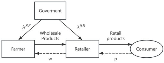
Figure 1.
Structure diagram of the agricultural product supply chain.
Retailers purchase agricultural products from farmers at a procurement price w and sell them to consumers at a retail price p, while the government provides subsidies to either retailers or farmers. Within this supply chain, the government, retailers, and farmers engage in a Stackelberg game, with the government acting as the leader, retailers as the second-mover, and farmers as followers. The decision-making sequence can be summarized as depicted in Figure 2.
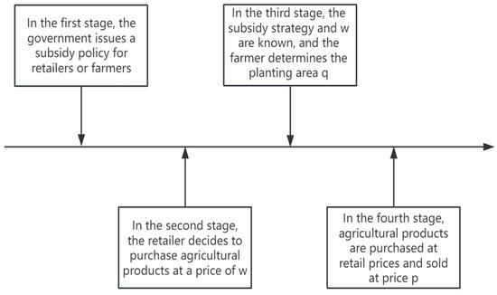
Figure 2.
Sequence of supply chain decisions.
In the first stage, the government issues subsidy policies for retailers or farmers; in the second stage, retailers determine the purchase price w of agricultural products from farmers based on the subsidy policy; in the third stage, farmers decide on planting area q considering the subsidy policy and procurement price w; in the fourth stage, retailers purchase and sell the agricultural products at price p.
3.2. Model Assumptions
Assuming that the decision variable for farmers is the planting area , agricultural production exhibits economies of scale, and marginal costs increase accordingly beyond a certain threshold of planting scale. Therefore, the production cost for farmers can be expressed as , where c represents the unit cost per unit area. Additionally, agricultural output is stochastic due to various uncertainties such as adverse weather conditions, pests and diseases, and seasonal variations. Therefore, the actual output per unit area can be expressed as , where is the random output rate, and , ( are the cumulative distribution function and probability density function of X, respectively). This study also considers constraints on farm size and risk aversion behavior; the total land area owned by farmers is limited to S, and farmers generally exhibit risk-averse tendencies with a risk aversion coefficient , where higher values indicate greater risk aversion.
This paper considers two subsidy strategies. The first involves the government providing area-based subsidies to farmers, referred to as the SF strategy. Under this strategy, farmers cultivating an area of q hectares are eligible for a subsidy of , where represents the subsidy rate per unit area. The second strategy entails the government subsidizing retailers based on purchase volume, which is designated as the SR strategy. Under the SR strategy, retailers receive a subsidy per unit purchased and sell to consumers at a price p, with the function expressed as , where denotes the choke price and represents the price sensitivity coefficient. Regardless of the chosen policy, the government faces fiscal budget constraints, with an upper limit denoted as . For clarity, subscripts F and R denote farmers and retailers, respectively, while superscripts SF and SR denote two subsidy strategies, namely those for farmers and retailers. A detailed explanation of the relevant symbols is provided in Table 1 to facilitate the understanding of model formulation and solution.

Table 1.
Symbols and explanations.
4. SF Strategy Model and Analysis
Under the SF strategy, the government provides a subsidy based on the farmers’ planting area q. The farmers’ profit function is:
Considering farmers’ risk aversion characteristics, this paper uses the CVaR method to describe the utility function of risk-averse farmers. Since the farmers’ decision variable, planting area, is constrained by their scale, the farmers’ objective function can be expressed as:
The profit function of retailers mainly includes the income obtained from selling agricultural products to consumers and the cost of purchasing agricultural products. Therefore, the profit function of retailers can be expressed as:
In the above set and , from which we can obtain the retailer’s expected profit function:
Therefore, the decision-making objective for retailers is:
The purpose of government subsidies is to maximize social welfare, which consists of four parts: the first part is farmers’ profits, the second part is retailers’ profits, the third part is consumer surplus, and the fourth part is government subsidies. Therefore, the specific form of social welfare is:
The expected social welfare under fiscal budget constraints is:
The government’s decision-making target is:
By using backward induction to figure out the best decisions for farmers, retailers, and the government, we can obtain the balanced results of how the supply chain works under the SF strategy, as shown in Lemma 1:
Lemma 1.
Under the SF strategy, the optimal planting area for farmers, the optimal purchase price for retailers, and the optimal subsidy rate for the government are shown in Table 2 below:
Table 2.
Farmers’ planting area, purchase prices, and government subsidy coefficients under the SF strategy.
Table 2 reveals two distinctive cases in the SF strategy. One is when S and , the purchase price converges to . This is because, in this case, the fiscal budget for subsidies is relatively ample. Even if retailers reduce the purchase price to zero to increase their profit margins, farmers are willing to accept this price because they can still obtain income through subsidies. In other words, although farmers directly receive the subsidies, retailers also benefit from them. The other special case occurs when S, resulting in a subsidy rate (). This situation arises because farmers with smaller landholdings do not require government subsidies. In other words, to increase social welfare and crop production through subsidies, the government should prioritize subsidies for larger-scale farmers.
Table 2 also shows that , which aligns with the findings established in the prior literature: when farmers own a small amount of land (S), both the purchase price offered by retailers and the planting area of farmers decrease as output uncertainty increases. Regarding farmers’ planting area, purchase prices, and government subsidy coefficients under the SF strategy, the number of agricultural products that farmers plant is affected by many factors. The above table mainly considers the equilibrium solution of planting area (q), purchase price (w) and government subsidy rate under different conditions, considering the land area of farmers and the government subsidy budget.
5. SR Strategy Model and Analysis
Under the SR strategy, retailers obtain government subsidies based on the volume of purchases, with a per-unit subsidy rate of . Under this strategy, farmers’ profit functions mainly include income from selling agricultural products to retailers and the costs of growing crops, specifically as follows:
Similarly, considering farmers’ risk aversion characteristics and scale constraints, their decision-making objectives can be calculated as follows:
Under the SR strategy, retailers receive subsidies based on the quantity purchased per unit, and their profit function is as follows:
The expected profit function for retailers is:
Therefore, the decision objective for retailers is:
Under this strategy, social welfare is:
The expected social welfare is defined as:
The government’s decision-making is formulated as the following optimization problem:
Similarly, using backward induction to find the optimal decisions for farmers, retailers, and the government, we can obtain the equilibrium results of supply chain operations under the SR strategy, as shown in Lemma 2:
Lemma 2.
Under the SR strategy, the optimal planting area for farmers, the optimal purchase price for retailers, and the optimal subsidy rate for the government are shown in Table 3 below:
Table 3.
Farmers’ planting area, purchase price, and government subsidy coefficient under the SR strategy.
Like the SF strategy, there is also a special case in the SR strategy, namely, when S, the government subsidy rate for retailers is , which means that when farmers’ land size is less than a certain level, there is no need to provide subsidies to retailers. In addition, indicate that retailers’ purchase prices and farmers’ planting areas decrease as output uncertainty increases. Regarding farmers’ planting area, purchase price, and government subsidy coefficient under the SR strategy, the number of agricultural products that farmers plant is affected by many factors. The above table mainly considers the equilibrium solution of planting area (q), purchase price (w) and government subsidy rate under different conditions, considering the land area of farmers and the government subsidy budget.
6. Government Subsidy Strategy Selection
Government subsidies usually improve overall social welfare, so this section uses this as a criterion for selecting the optimal strategy.
The calculations conducted above have established the ideal decisions and their corresponding value ranges for each member under the two techniques, with the ranges principally categorized by varying farm sizes (S) and fiscal budgets (B). The comparison of the two procedures must occur within the feasible intervals of each optimal solution. This results in seven separate regions A1–A7 (shown in Figure 3, where , when , , with the hierarchy ) and the associated best solutions for both methods inside each region (Table 4). This study evaluates the SF and SR strategies across seven locations and identifies the process that maximizes social welfare as the ideal choice. For clarity, we define as small farmer scale, as moderate scale; as limited budget, as adequate budget, and as excessive budget.
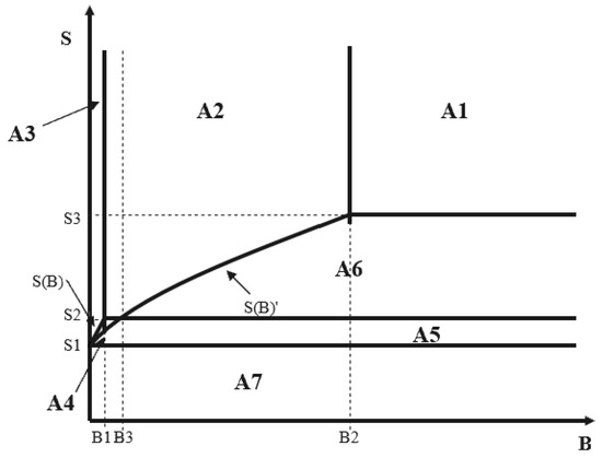
Figure 3.
Strategy selection area, with black solid lines indicating the boundaries of the area.
Table 4.
Strategy comparison areas and their corresponding optimal solutions.
Proposition 1.
- ①
- When, . To maximize social welfare, the government should adopt the farmer subsidy policy (SF strategy). Under this condition: .
- ②
- When with , . The government should choose the SF strategy.
Proposition 1 states that when or with , as shown in Figure 3, the government’s fiscal budget is small (), and the scale of farmers is not small (). Choosing the SF strategy to subsidize farmers rather than retailers can achieve higher social welfare. This is because, given the uncertainty of output and the higher the risk aversion of farmers, the lower the purchase price. Direct subsidies to farmers can encourage them to expand their planting area and ensure the yield of crops, thereby achieving higher social welfare. Furthermore, in the regional selection of subsidizing farmers, farmers and retailers expect higher profits than subsidizing retailers.
Proposition 2.
- ①
- When, , meaning that the SR strategy yields higher social welfare than the SF strategy, and .
- ②
- When , similar welfare dominance holds: with:. The government should choose the SR strategy.
- ③
- When with , , at which point the government should also choose the SR strategy.
For parameter regions where with or (B,S) ∈ A1∪A6, the SR strategy generates higher social welfare than SF, given sufficient fiscal budgets. This occurs because SF’s direct subsidies to farmers and retailers depress purchase prices ( in extreme cases), reducing planting incentives and output. In contrast, SR retailer subsidies elevate procurement price (), which expands cultivation areas () and enhances welfare. Additionally, in these regions, farmers and retailers under the SR strategy have higher expected profits than those under the SF strategy.
Proposition 3.
When, the effects of the SF and SR subsidy strategies are the same, i.e., . When , there is no need for the government to provide subsidies to farmers or retailers.
Proposition 3 states that when , the scale of farming is moderate and there are no fiscal constraints. At this point, the effects of SR and SF subsidies are the same, i.e., social welfare is the same under both strategies, and farmers will fully utilize their land (). When , the scale of farming is small (), and the government does not need to provide subsidies to farmers and retailers because farmers will always choose to utilize their land () fully, and the government does not need to provide subsidies to encourage them to utilize their land to increase output fully.
Furthermore, under conditions of moderate farm scale and constrained fiscal budgets (within region A4), the relative social welfare performance of both strategies exhibits parametric dependence: for small-scale farms, welfare dominance shifts toward the SR strategy as budget B increases; for large-scale farms, the SF strategy becomes superior with expanding B.
7. Numerical Analysis
7.1. The Impact of Different Subsidy Budgets
To further investigate the impact of the fiscal budget (B) on subsidy effectiveness and validate the conclusions drawn above, the numerical examples are presented below. Parameter values are set as a = 0.407, b = 0.022, c = 0.015, = 0.029, = 0.5with farm size fixed at S = 11 (). Given this fixed scale, the fiscal budget B becomes the sole independent variable. The numerical analysis results are shown in Figure 4 (solid lines represent SF, and dashed lines represent SR). As shown in Figure 4, when the government fiscal budget is insufficient (), SF is superior to SR. When the fiscal budget is adequate (), SR is superior to SF.
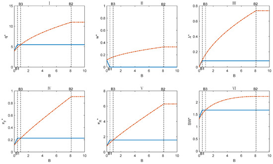
Figure 4.
Numerical analysis results of the impact of different fiscal budgets (when S = 11) on the supply chain. ((I), (II), (III), (IV), (V) and (VI) respectively show how q*, w*, changes under the SF strategy when the fiscal subsidy B changes).
Under the SF strategy, as B increases, farmers will expand their planting area (Figure 4I), but retailers will lower their purchase prices (Figure 4II). This is because the subsidy is applied to farmers, and retailers are not direct beneficiaries. Therefore, to transfer profits, retailers will lower their purchase prices, even to zero (at this point, ), and farmers can still rely entirely on subsidies as their source of income. When the subsidy exceeds , increasing the fiscal budget under the SF strategy no longer has any effect.
Under the SR strategy, the government chooses to subsidize retailers, and within a specific range, the larger the subsidy budget, the higher the acquisition price (Figure 4II). Although there is no direct subsidy to farmers, this significantly encourages farmers to expand their planting area and increase their income (Figure 4IV), far exceeding the planting area and expected profits of farmers under the SF strategy. For retailers, as the subsidy budget increases, although the purchase price rises, the SR strategy remains more advantageous than the SF strategy, yielding higher profits and social welfare (Figure 4V,VI). However, to fully leverage the advantages of the SR strategy, a higher subsidy rate than under the SF strategy is required (Figure 4III), which may increase government spending and create fiscal pressure. Additionally, once the subsidy budget exceeds a certain threshold, , further increases in the budget will no longer be effective under the SF strategy. Therefore, the government should avoid unquestioningly increasing fiscal budgets and instead focus on moderate subsidies.
In summary, the numerical analysis in this section shows that when national finances are tight and subsidy budgets are limited, subsidizing farmers can result in higher social welfare. However, subsidizing retailers is the wiser choice when national finances are abundant.
7.2. The Impact of Output Uncertainty
To study the impact of uncertainty on the effectiveness of subsidies, we perform numerical simulations using the following parameter constellation: a = 0.407, b = 0.022, c = 0.015, = 0.5, S = 11, and B = 0.4. Figure 5 presents the comparative results (SF: solid lines; SR: dashed lines). The results demonstrate that the SF strategy outperforms the SR strategy in terms of addressing output uncertainty.
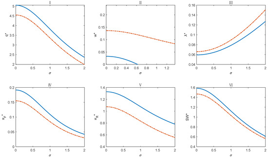
Figure 5.
Numerical analysis results of the impact of output uncertainty on the supply chain. ((I), (II), (III), (IV), (V) and (VI) respectively show how q*, w*, changes under the SR strategy when the fiscal subsidy B changes).
Figure 5 illustrates that, except for the subsidy rate, which increases with the level of production uncertainty (Figure 5III), all other variables exhibit a corresponding decline. When there is high output uncertainty, the government anticipates enhancing social welfare by increasing the subsidy rate to encourage farmers and retailers. Figure 5II illustrates that, irrespective of the rise in output uncertainty, the purchase price under the SR strategy consistently exceeds that of the SF strategy. The subsidy in the SR strategy directly impacts retailers. In conditions of significant uncertainty, risk-averse farmers typically decrease their planting area (Figure 5Ⅰ), prompting acquirers to offer a higher purchasing price relative to the SF strategy to encourage farmers to cultivate crops and secure production. According to the SF strategy, farmers’ cultivation areas and anticipated revenues (Figure 5IV) constantly surpass those associated with the SR strategy. This suggests that under conditions of high output uncertainty, the SF strategy surpasses the SR strategy in augmenting planting fields, securing output, and enhancing farmers’ income while providing superior incentive effects. Despite the lower purchase price associated with the SF strategy compared to the SR strategy, high-output retailers can attain greater predicted profits under the SF strategy (Figure 5V), and social welfare is also enhanced under the SF strategy at this juncture (Figure 5VI).
In summary, the numerical analysis in this section shows that the SF strategy is superior to the SR strategy in responding to output uncertainty. When farmers’ crop output is highly uncertain, the government should subsidize farmers to achieve higher output and social welfare and effectively help farmers increase their income.
7.3. The Impact of Risk Aversion Degree
To explore the impact of risk aversion on the choice of government subsidy strategies, this section conducts a numerical analysis to further study the changes in social welfare under the two strategies at different risk levels for farmers. Here, the numerical values are set as a = 0.407, b = 0.022, c = 0.015, S = 11, and the parameter takes values of 0.1, 0.5, and 0.9, respectively. The analysis results are shown in Figure 6.
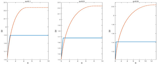
Figure 6.
Impact of risk aversion on social welfare (solid line represents SF, dotted line represents SR).
Figure 6 illustrates that, in the context of risk aversion, when the fiscal budget B is constrained, the SF strategy outperforms the SR strategy. Furthermore, a lower degree of risk aversion correlates with a diminished disparity in social welfare between the two strategies under conditions of budgetary insufficiency; conversely, when the fiscal budget is sufficiently ample, the SR strategy exhibits a marked advantage over the SF strategy. Nonetheless, when risk aversion escalates, societal welfare diminishes under both techniques. This numerical study suggests that the government should implement the SF strategy when farmers demonstrate risk aversion and an inadequate fiscal budget. If the budget is sufficiently ample, the SR strategy should be selected. An escalation in risk aversion diminishes social welfare under both solutions, indicating that neither SF nor SR can adequately alleviate the adverse impacts of farmers’ risk aversion. Agricultural insurance subsidies could potentially resolve the situation; nevertheless, additional research is required.
8. Conclusions and Future Research Direction
This paper constructs a three-level supply chain of farmers, retailers, and the government. Under constraints on farm size and subsidy budgets, it examines the optimal decisions of supply chain members under two subsidy strategies: one where the government subsidizes farmers based on planting area and another where it subsidizes retailers based on purchase volume. The paper also analyzes the impact of factors such as farmers’ land size and risk aversion, subsidy budgets, and output uncertainty on strategy selection and subsidy effectiveness. The conclusions are as follows:
- 1.
- When farmers have a large scale (i.e., the land area owned by the farmers, denoted as S, is greater than or equal to ), the SF strategy is superior to the SR strategy when the fiscal budget is relatively limited. When the fiscal budget is relatively abundant, the SR strategy is superior to the SF strategy.
- 2.
- When farmers have a moderate land scale and no budget constraints, the subsidy effects of the SF and SR strategies are the same.
- 3.
- When farmers have a small scale (i.e., the land area owned by the farmer, denoted as S, is less than ), the government does not need to provide subsidies.
- 4.
- When the subsidy budget is excessive, further increases will yield no additional benefits. Thus, the government should adjust the subsidies appropriately, considering real-world conditions.
- 5.
- The SF strategy is superior to the SR strategy in addressing output uncertainty. If the output uncertainty of the crops farmers plant is high, the government should subsidize farmers.
- 6.
- Considering farmers’ risk aversion, if the budget is limited, the SF strategy is more advantageous; if the budget is ample, the SR strategy is more advantageous. The higher the degree of risk aversion, the lower the social welfare under both strategies, indicating that neither strategy can effectively mitigate the negative impacts of farmers’ risk aversion.
The purpose of this study is to provide a reference for the government in selecting subsidy strategies. However, there are still some shortcomings. Agricultural products have long production cycles and face high natural uncertainties (weather, pests and diseases) and market uncertainties (changes in demand, competition from substitutes and policy adjustments). The risk distribution is often asymmetric and fat-tailed, making it difficult to model precisely. On the other hand, in the process of model derivation, we only based this on the linear demand assumption that demand is only related to price. However, in the actual operation of the agricultural supply chain, demand may be affected by other non-price factors, such as the amount of subsidy, arrival time, agricultural product quality and many other factors affecting the operation of the agricultural supply chain. For example, a series of notices issued by the state mention the hope of improving the quality of food supply through measures such as subsidies, but this study does not consider the impact of subsidies on factors such as food quality, which requires further research in the future.
Author Contributions
Conceptualization, W.C. and X.H.; Methodology, W.C.; Software, W.C.; Validation, W.C. and X.H.; Formal Analysis, W.C.; Investigation, X.H.; Resources, X.H.; Data Curation, X.H.; Writing—Original Draft Preparation, X.H.; Writing—Review & Editing, W.C.; Visualization, X.H.; Supervision, W.C.; Project Administration, W.C.; Funding Acquisition, W.C. All authors have read and agreed to the published version of the manuscript.
Funding
This research received no external funding.
Data Availability Statement
Not applicable.
Conflicts of Interest
The authors declare no conflicts of interest.
References
- Zhang, X.M.; Zhu, J.H.; Dan, B. Consideration of subsidies and public welfare in the incentives for fresh cold chain preservation investments. Syst. Eng.-Theory Pract. 2022, 42, 738–754. [Google Scholar]
- Peng, H.J.; Pang, T. Research on the financing and operation strategies of contract agriculture supply chain under agricultural subsidy policies. J. Manag. Eng. 2020, 34, 155–163. [Google Scholar]
- Zhou, Y.J.; Zheng, D.; Ye, X. Decision-making and coordination of the three-level agricultural product supply chain considering poverty alleviation preferences. Control Decis. 2020, 35, 2589–2598. [Google Scholar]
- Akkaya, D.; Bimpikis, K.; Lee, H. Government interventions to promote agricultural innovation. Manuf. Serv. Oper. Manag. 2021, 23, 437–452. [Google Scholar] [CrossRef]
- Zhu, J.H.; Zhang, X.M.; Dan, B.; Liu, M.; Ma, S. Government subsidy strategies for fresh agricultural products considering financial constraints under uncertain demand. Chin. J. Manag. Sci. 2022, 30, 231–242. [Google Scholar]
- Liu, H. Finding the way out to African swine fever: Analysis of Chinese government’s subsidy programs to farms and consumers. Comput. Ind. Eng. 2021, 160, 107543. [Google Scholar] [CrossRef]
- Yu, X.; Zhang, W.G.; Liu, Y.J. Research on the subsidy mechanism of agricultural product supply chain based on agricultural insurance. J. Manag. Stud. 2017, 14, 1546–1552. [Google Scholar]
- Yu, X.; Zhang, W.G.; Liu, Y.J. Research on the coordination mechanism of order agriculture based on relative floating prices and government subsidies. J. Manag. Eng. 2020, 34, 134–141. [Google Scholar]
- Huang, J.H.; Lin, Q. Government Subsidy Mechanism in Contract-farming Supply Chain Financing under Loan Guarantee Insurance and Yield Uncertainty. Chin. J. Manag. Sci. 2019, 27, 53–65. [Google Scholar]
- Ye, F.; Cai, Z.; Chen, Y.J.; Li, Y.; Hou, G. Subsidize farmers or bioenergy producer? The design of a government subsidy program for a bioenergy supply chain. Nav. Res. Logist. (NRL) 2021, 68, 1082–1097. [Google Scholar] [CrossRef]
- Pu, X.J.; Lai, D.L.; Jin, D.L. Subsidy-by-Quantity vs. Subsidy-by-Price: Optimal Government Strategies in E-Commerce Poverty Alleviation. Chin. J. Manag. Sci. 2023, 8, 32–40. [Google Scholar]
- Peng, H.J.; Pang, T. Optimal strategies for a three-level contract-farming supply chain with subsidy. Int. J. Prod. Econ. 2019, 216, 274–286. [Google Scholar] [CrossRef]
- Bai, S.Z.; Wang, Y.G.; Zheng, S.H.; Huang, S.J. Consideration of risk aversion and negotiation power in the green investment mechanism of agricultural product supply chains. Control Decis. 2022, 37, 1862–1872. [Google Scholar]
- Fu, H.Y.; Dan, B. Contract design of “Company-Farmer” orders under adverse weather conditions. Chin. J. Manag. Sci. 2015, 23, 128–137. [Google Scholar]
- Ye, F.; Lin, Q.; Li, Y.N. Contract mechanism for coordinating “company-farmer” type order agriculture supply chain based on CVaR. Syst. Eng.-Theory Pract. 2011, 31, 450–460. [Google Scholar]
- Lin, Q.; Fu, W.H.; Wang, Y.J. Internal Financing Decisions in the “Company-Farmer” Model of Agricultural Supply Chains. Syst. Eng.-Theory Pract. 2021, 41, 1162–1178. [Google Scholar]
- Yan, N.; Sun, B.; Zhang, H.; Liu, C. A partial credit guarantee contract in a capital-constrained supply chain: Financing equilibrium and coordinating strategy. Int. J. Prod. Econ. 2016, 173, 122–133. [Google Scholar] [CrossRef]
- Ning, J. Strategic trade credit in a supply chain with buyer competition. Manuf. Serv. Oper. Manag. 2022, 24, 2183–2201. [Google Scholar] [CrossRef]
- Lin, Q.; Xiao, Y. Retailer Credit Guarantee in a Supply Chain with Capital Constraint under Push & Pull contract. Comput. Ind. Eng. 2018, 125, 245–257. [Google Scholar] [CrossRef]
- Kouvelis, P.; Zhao, W. Financing the Newsvendor: Supplier vs. Bank, Optimal Rates, and Alternative Schemes; Olin Business School, Washington University: St. Louis, MO, USA, 2008. [Google Scholar]
- Huang, J.; Yang, W.; Tu, Y. Supplier credit guarantee loan in supply chain with financial constraint and bargaining. Int. J. Prod. Res. 2019, 57, 7158–7173. [Google Scholar] [CrossRef]
- Hua, S.; Liu, J.; Cheng, T.C.E.; Zhai, X. Financing and ordering strategies for a supply chain under the option contract. Int. J. Prod. Econ. 2019, 208, 100–121. [Google Scholar] [CrossRef]
- Gao, G.X.; Fan, Z.P.; Fang, X.; Fong, L.Y. Optimal Stackelberg strategies for financing a supply chain through online peer-to-peer lending. Eur. J. Oper. Res. 2018, 267, 585–597. [Google Scholar] [CrossRef]
- Xu, S.; Fang, L. Partial credit guarantee and trade credit in an emission-dependent supply chain with capital constraint. Transp. Res. Part E Logist. Transp. Rev. 2020, 135, 101859. [Google Scholar] [CrossRef]
- Wu, S.M.; Chan, F.T.S.; Chung, S.H. The impact of buyback support on financing strategies for a capital-constrained supplier. Int. J. Prod. Econ. 2022, 248, 108457. [Google Scholar] [CrossRef]
- Wang, J.; Wang, K.; Li, X.; Zhao, R. Suppliers’ trade credit strategies with transparent credit ratings: Null, exclusive, and nonchalant provision. Eur. J. Oper. Res. 2022, 297, 153–163. [Google Scholar] [CrossRef]
- Wang, C.; Chen, X.; Jin, W.; Fan, X. Credit guarantee types for financing retailers through online peer-to-peer lending: Equilibrium and coordinating strategy. Eur. J. Oper. Res. 2022, 297, 380–392. [Google Scholar] [CrossRef]
- Shi, J.; Du, Q.; Lin, F.; Lai, K.K.; Cheng, T.C.E. Optimal financing mode selection for a capital-constrained retailer under an implicit bankruptcy cost. Int. J. Prod. Econ. 2020, 228, 107657. [Google Scholar] [CrossRef]
- Shen, B.; Wang, X.; Cao, Y.; Chen, B. Financing decisions in supply chains with a capital-constrained manufacturer: Competition and risk. Int. Trans. Oper. Res. 2020, 27, 2422–2448. [Google Scholar] [CrossRef]


Disclaimer/Publisher’s Note: The statements, opinions and data contained in all publications are solely those of the individual author(s) and contributor(s) and not of MDPI and/or the editor(s). MDPI and/or the editor(s) disclaim responsibility for any injury to people or property resulting from any ideas, methods, instructions or products referred to in the content. |
© 2025 by the authors. Licensee MDPI, Basel, Switzerland. This article is an open access article distributed under the terms and conditions of the Creative Commons Attribution (CC BY) license (https://creativecommons.org/licenses/by/4.0/).