Article

Spatiotemporal Characteristics of Land Use Carbon Budget and Carbon Balance Capacity in Karst Mountainous Areas: A Case Study Using Social Network Analysis

1
College of Public Administration, Guizhou University of Finance and Economics, Guiyang 550025, China
2
Huaxi District Bureau of Natural Resources, Guiyang 550025, China
*
Author to whom correspondence should be addressed.
Systems 2025, 13(8), 686; https://doi.org/10.3390/systems13080686
Submission received: 16 June 2025 / Revised: 29 July 2025 / Accepted: 5 August 2025 / Published: 12 August 2025

Abstract

Collaborative carbon regulation in Karst mountains critically reconciles socio-ecological conflicts. While intercity linkages drive spatial carbon heterogeneity, prior studies have focused on administrative-scale accounting, neglecting systematic spatial association network (SAN) analysis. Integrating SAN and geospatial detector models, we reveal county-level carbon balance dynamics in Guizhou, China (2000–2020). The key findings show the following: provincial carbon emissions rose 53% (0.96 to 1.47 × 10⁸ t) against a 15% sequestration decline (0.67 to 0.57 × 10⁸ t); emission networks shifted from single-core clustering to the axial Liupanshui–Guiyang–Tongren corridor, while sequestration networks retained peripheral ecological dominance; carbon balance capacity (CBC) exhibited an inverted C-shaped pattern (higher in the southeast, lower in the central–west) with westward centroid migration; and electricity consumption dominated spatial heterogeneity, with synergistic nighttime light–PM2.5 interactions showing strongest nonlinear enhancement. Notably, Jianhe County maintained peak CBC (16.5) via forest carbon sinks, whereas Shiqian County suffered the steepest decline due to industrial encroachment. This work pioneers dynamic carbon coupling analysis in fragile ecosystems, offering transdisciplinary tools for global “dual-carbon” governance.

1. Introduction

Reducing carbon dioxide emissions and strengthening carbon sinks are crucial for mitigating climate change and achieving carbon neutrality. Carbon budget research has emerged as a core scientific issue for balancing regional development and ecological conservation. The IPCC Sixth Assessment Report [1,2] notes that atmospheric carbon dioxide concentrations have increased by 48% in 2020 compared to pre-industrial levels. As the world’s largest carbon emitter [3], China’s emission reduction pathways hold critical significance for global climate governance [4]. However, existing studies have predominantly focused on national or provincial scales [5,6], with inadequate attention to county-level units, especially in topographically fragmented and ecologically vulnerable Karst mountainous areas, which account for 12% of the global land area [7,8]. Despite their high carbon sink potential, these regions have long been regarded as “blind spots” in carbon cycle research due to data and methodological limitations [9]. Taking Guizhou—a typical Karst province in Southwest China—as an example, its unique geographical landscape and rapid industrialization create a sharp contradiction, thereby providing a distinctive case for analyzing the spatiotemporal dynamics of carbon sources and sinks [10]. The current research focuses on carbon cycle processes at multiple scales. The academic community has systematically explored the evolution mechanisms of carbon fluxes under human activity disturbances and has made significant progress, especially in understanding the dynamic response patterns of regional carbon emissions and absorptions. Cai, et al. [11] established the Chinese High-Resolution Emission Database (CHRED) and, taking the entire spatial scale as the research object, achieved the integrated application of point-source and gridded emission data with socioeconomic elements. Marchi, et al. [12] developed a regional carbon cycle simulation framework and conducted empirical analysis using the Province of Siena, Italy, as a case study. Wu, et al. [13] employed logarithmic mean division index (LMDI) decomposition to develop a carbon emission decoupling framework, analyzing the multidimensional effects of economic drivers across 30 Chinese provinces. Kumar and Sen [14] conducted an empirical study using India’s multi-gradient cities as samples, revealing the synergistic constraint mechanisms between population size and density indices. Xu, et al. [15] conducted a study on the spatial differentiation of carbon emissions and analysis of driving mechanisms using China’s prefecture-level cities as the research object. While current carbon budget research has established multi-scale analytical frameworks, it predominantly focuses on macro-level tiers such as nations, regions, or cities. Research on carbon metabolism mechanisms at the county level remains a significant blind spot. China’s county-level units exhibit unique differentiation patterns in industrial structure evolution, spatial coupling of carbon sources and sinks, and carbon sequestration substrate heterogeneity [16]. This endows county-level carbon balance research with dual values: theoretically, it can reveal interactions between natural and social systems through multi-scale model coupling; practically, it provides spatial decision-making benchmarks for differentiated carbon neutrality pathways at the county level [17].
Existing research has inadequately addressed the spatial heterogeneity of carbon budgets/balances and network correlation mechanism–systematic analysis from the perspectives of spatial network structure, and regional disparities remain notably insufficient. This fundamentally limits the precision of policy instruments in targeting regional carbon emission governance. As a key entry point for addressing this challenge, the research value of the Spatial Association Network for Carbon Budgets/Balances (SAN) is manifested in two dimensions: it can both quantitatively characterize spatiotemporal differentiation characteristics among geographic units and reveal interaction mechanisms within regional systems. An in-depth analysis of its spatial association characteristics, driving mechanisms, and spillover effects not only enhances the accuracy of carbon balance accounting and monitoring effectiveness but also provides a scientific basis for identifying the cross-regional impacts of emission reduction policies in policy making, thereby supporting the establishment of interregional emission reduction collaboration mechanisms and optimal allocation of carbon resources. Advancements in spatial analysis methodologies have systematically enhanced the academic community’s comprehension of carbon balance spatiality. Methods such as spatial autocorrelation and hotspot analysis have been employed to reveal the spatiotemporal agglomeration patterns of carbon emissions, while econometric tools like the Environmental Kuznets Curve [18] and Spatial Durbin Model [19] have played pivotal roles in studying spatial spillover effects. However, existing methodologies exhibit notable limitations. Traditional spatial analysis over-relies on geographical distance weights, inadequately characterizing the action mechanisms of non-geographical factors such as industrial policies and market economies [20]. Spatial econometric models are constrained by subjectivity in specifying spatial weight matrices, leading to substantial uncertainties in research conclusions [21]. Notably, regional carbon balance systems are influenced by interwoven multidimensional factors—economic structure, technological level, and policy orientation [22,23,24]—with their spatial associations having transcended simple geographical proximity to form complex network coupling configurations. Yu, et al. [25] further demonstrated that geographical factors alone are unable to explain the network linkage characteristics of carbon balance in urban agglomerations. Currently, the academic community lacks a systematic understanding of key scientific questions regarding the spatial networks of carbon budgets/balances at the county level; notably, research deficiencies persist in network structural characteristics, node functional effects, and evolutionary patterns of spatiotemporal heterogeneity. These knowledge gaps directly hinder the scientific comprehension of carbon system complexity, urgently demanding breakthroughs through interdisciplinary methodological integration and innovations in network analysis techniques.
Studies employ various methodologies to explore driving factors, such as the grey correlation model [26] and geographical weighted regression (GWR) model [27]. However, traditional correlation and regression approaches often overlook the interconnections and coupling effects between factors, neglecting the spatial heterogeneity in driving factor impacts [28]. These methods struggle to capture the nonlinear synergies between NDVI and industrial structure while failing to integrate the “core–periphery” structure of carbon flow networks, thus leading policy designs to deviate from practical needs.
Consequently, addressing the gaps in existing research regarding the spatial heterogeneity of carbon budgets/balances, network correlation mechanisms, and systematic analysis at the county level, this study aims to answer the following core research questions. (1) How can the spatiotemporal evolution characteristics of land use carbon budgets be quantitatively characterized at the county level in Guizhou Province? (2) How does the structure of the spatial association network of carbon budgets evolve among county-level units, and what are the patterns regarding core nodes and their functional roles? (3) Which driving factors and their nonlinear interactions dominate the spatial differentiation of Carbon Balance Capacity (CBC) at the county level? To address these questions, this research focuses on the 88 county-level administrative units in Guizhou Province (2000–2020). We integrate data from the China Emission Accounts and Datasets (CEADs), Landsat remote sensing imagery [29], and socioeconomic statistics to construct a full-chain framework of “carbon accounting–network analysis–driving factor detection.” By coupling the gravity model with Social Network Analysis (SNA), we quantify the inter-county carbon flow network structure [30]. The GeoDetector model is employed to analyze the nonlinear interaction effects of factors such as NDVI and industrial structure [31]. Furthermore, standard deviational ellipses are used to reveal the spatial evolution trajectories of CBC, ultimately proposing differentiated policy pathways [32,33]. This framework offers a novel perspective and methodological toolkit for studying carbon budgets in Karst mountainous counties, and its replicable technical approach provides a reference for achieving “dual-carbon” goals in global ecologically vulnerable regions.

2. Materials and Methods

2.1. Study Area

Guizhou Province (103°36′~109°35′ E, 24°37′~29°13′ N), situated in the core of Southwest China, stands as a quintessential inland mountainous province. Bounding Yunnan to the west, Sichuan and Chongqing to the north, Hunan to the east, and Guangxi to the south, it administers 88 county-level divisions across a territorial expanse of 176,000 km2. The regional topography adheres to the characteristic “eight parts mountains, one part water, one part farmland” configuration, with 92.5% of its landmass composed of mountains and hills, over 70% of which exhibit Karst geo-morphology, forming a pivotal hydrological divide between the Pearl River–Xijiang system and the upper Yangtze River basin. Unique geological structures have shaped a west-high, east-low terrain tilting northeastward and southeastward, which has also engendered notable vulnerability in regional ecosystems. Between 2000 and 2017, while achieving an annual GDP growth rate exceeding 10%, Guizhou exhibited a development pattern characterized by pronounced high energy consumption, carbon emissions, and pollution. This traditional extensive growth path has not only exacerbated the already fragile ecological carrying capacity in Karst regions but also posed severe challenges to regional ecological security patterns and the low-carbon sustainable development of both the Yangtze River Economic Belt and Pearl River–Xijiang Economic Belt [34]. Balancing ecological conservation and economic growth has emerged as a pressing core issue to be managed if the province is to achieve high-quality development (Figure 1).

2.2. Data Sources

Taking the 88 county-level administrative units in Guizhou Province as the research scope, missing data were imputed using two methods: mean values from neighboring counties for spatial continuity and linear interpolation for temporal consistency. Employing a 2000–2020 research period divided into 5-year intervals, incorporating multi-source data (land use, socioeconomic indicators, digital elevation models (DEM), administrative division boundaries, and climatic datasets). Data sources included county-level CO2 emission data derived from the 1997–2017 China County-Level CO2 Emission Inventory of the China Emission Accounts Datasets and socioeconomic data (2000–2020) for carbon emission and sink calculations primarily derived from authoritative national-level statistical resources, including the Guizhou Statistical Yearbook, Guizhou Bulletin on National Economic and Social Development, and China Statistical Yearbook, thus ensuring data reliability and research accuracy. Guizhou’s 2000–2020 land use data, derived from Landsat remote sensing imagery, were classified into six categories—cropland, forest, grassland, water bodies, urban land, and unused land—at 30 m × 30 m resolution using visual interpretation integrated with a random forest classifier. Agricultural data were sourced from the Guizhou Statistical Yearbook, while climatic data originated from the National Meteorological Science Data Center of the China Meteorological Administration. The maps used in this study were created based on standard maps downloaded from the National Administration of Surveying, Mapping and Geoinformation’s standardized map service portal (map approval number: GS(2024)0650), with no modifications to the base maps.

2.3. Methods

(1) Carbon emission calculation
Given that the China Emission Accounts and Datasets only include the 1997–2017 county-level CO2 emission inventory, this study adopted the methodology proposed by Shuoshuo, et al. [35], employing three approaches to estimating and comparing county-level carbon emissions in the Dongting Lake Basin in 2020.
After comparison, the approach of calculating growth factors from urban carbon emission datasets to estimate county-level emissions proved more accurate, with the formula as follows:
R = C Y 2020 C Y 2015 C Y 2015
C F 2020 = C F 2015 × 1 + R
In the formula, R represents the urban carbon emission growth factor for 2015–2020; C Y 2020 and C Y 2015 denote urban carbon emissions in 2020 and 2015, respectively; and C F 2020 and C F 2015 signify county-level carbon emissions in 2020 and 2015, with C F 2015 derived from the CEADs county-level emission inventory.
(2) Carbon sequestration calculation
The carbon sequestration formula for various carbon sink land uses is as follows:
C l = L i × δ i
In the formula, C l denotes the CO2 sequestration amount; L i represents the area of various types of land; and δ i signifies the carbon sequestration rate per unit area of various types of land. Based on existing research of Shen [36], the carbon sequestration coefficients for different land types are as follows: forestland at 5.81 t/(hm2·a), grassland at 0.021 t/(hm2·a), water bodies at 0.253 t/(hm2·a), and unused land at 0.005 t/(hm2·a).The calculation for crop carbon sequestration is
H c = i I i = i Z i × 1 P i × Y i H i
In the formula, the total carbon sequestration of crops is represented by symbol H c . The carbon absorption of the i-th crop is denoted I i . The carbon absorption rate of the i-th crop is expressed as Z i . Moisture content is represented by P i , yield by Y i , and economic coefficient by H i . For data processing, grain crop parameters (rice, wheat, and other cereals) were characterized using average values of their respective indicators, while oil crop parameters adopted mean values from peanut and sesame data. Specific parameter values are listed in Table 1.

3. Spatial Network Analysis of Carbon Budgets

This study utilized the Gravity Model in ArcGIS 10.8 to develop a spatial association network framework for characterizing the spatial correlation structure of Guizhou’s carbon budgets. Within this framework, county-level administrative units are treated as network nodes (with their administrative center coordinates as XY parameters), and inter-county carbon-related interactions are defined as connecting edges. Social network analysis (SNA) was selected for network parsing given that conventional spatial correlation models, which overly rely on geographical proximity weights, are inadequate for capturing non-geographical interactions, which are particularly critical in Karst regions with fragmented topography. By quantifying metrics including node centrality and network density, SNA enables the identification of “core–periphery” structures and evolutionary trajectories of carbon associations, which remain unrecognized in traditional analytical frameworks. Complementarily, the GeoDetector model was employed for driving factor analysis to address the limitation of conventional regression models in neglecting spatial heterogeneity and nonlinear factor interactions. Through calculating q-values, it precisely identifies synergistic effects that underpin carbon balance dynamics, thereby enhancing the mechanistic depth of spatial analysis. Corresponding indicators were subsequently applied to explore the spatial patterns, interaction logics, and evolutionary trends of the overall network and individual nodes.

3.1. Gravity Model

The essence of the gravity model lies in the intensity of the gravitational force between two evaluated objects, which is jointly determined by their scale magnitudes and spatial distances. Moreover, we can present the changing trends of spatial correlations using cross-sectional data. This paper applies this model to depict the spatial correlation patterns of the carbon budget in order to construct a spatial association network. The spatial association network of the carbon budget in Guizhou Province is composed of the interrelationships between carbon budgets in 88 county-level regions. This spatial network comprises two main constituent elements, namely the “nodes” and the “connections”. The “nodes” represent each county in Guizhou Province, while the “connections” refer to the spatial correlation relationships between carbon budgets among these counties. The specific calculation is as follows [37]:
Y i j = k T i T j D i j 2
In the formula, “I” and “j” mark County i and County j, respectively; Yij represents the quantitative expression of the gravitational force between County I and County j. A larger value indicates stronger gravitational force between cities. Ti and Tj denote the carbon budgets of land use in City i and City j, serving as key indicators for measuring the carbon cycle in urban land use processes. Dij denotes the distance between the geometric centers of two cities (unit: kilometers), defining their relative positional relationship in spatial distribution. Within this formula framework, the gravitational constant k is set to “1”.
Using the average correlation intensity (y*) of land-use carbon budgets across five periods from 2000 to 2020 as the threshold, values exceeding y* are retained to signify a connection in the carbon budget correlation network between two counties, while those below y* are set to 0, indicating no spatial correlation. The specific calculation is as follows:
I = c i j = 1 , Y i j > y * 0 , Y i j y *
In the formula,” I “denotes a binary matrix; c i j represents its element; Y i j signifies the gravitational value between County i and County j; and y* is the preset threshold.

3.2. Social Network Analysis Method

Social network analysis (SNA) transforms qualitative structural attribute data into matrix format by constructing network correlation models, enabling intuitive representation of cities’ spatial correlation status and network positions within the framework [38]. This study employs social network analysis to derive a binary relational matrix based on Equation (6), deeply analyzing the spatial association network characteristics of land-use carbon budgets in Guizhou Province from two dimensions: overall network attributes and individual network attributes.
(1) Overall network attributes
This study employs network density metrics to characterize the properties of the overall network structure. As one of the core indicators for spatial association networks, network density effectively measures the tightness of connections between nodes: a higher value indicates stronger spatial correlations between cities and more significant mutual influence [39]. The specific calculation formula for network density is as follows:
D = 2 M N N 1
In the formula, M denotes the number of spatial correlation relationships in land-use carbon budgets, while N represents the number of node counties.
(2) Individual network attributes
This study employs two indicators—degree centrality and betweenness centrality—to characterize the status and roles of network nodes. In the spatial association network, degree centrality measures the position of a city in a network by counting the number of direct spatial connections it has with other cities. A higher value indicates a more central position of the city within the network, signifying its role as a central actor [40,41]. The specific calculation method is as follows:
D = d i N 1
In the formula, d i denotes the number of direct associations for County i, while N represents the total number of node counties.
Intermediary centrality, a key indicator for measuring the structural position of cities in regional spatial association networks, is used to assess the degree to which a county acts as an intermediary in the spatial connections between other counties. In the network framework, if County i lies on the shortest path between any Counties j and k, the spatial connection between j and k must be mediated by i, indicating that County i performs an indispensable intermediary role in their association. A higher intermediary centrality value indicates a more significant mediating role in the spatial association network, with its calculation formula provided below.
Z = 2 e N r N g e r i / g e r 3 N 2 3 N + 2
In this formula, g e r i denotes the shortest association paths between Nodes e and r that pass through Node i. The conditions specify that e ≠ r ≠ I and e < r. g e r denote the shortest association paths between Nodes e and r, while N represents the total quantity of node cities.

3.3. Calculation of Carbon Balance Capacity

The Ecological Carbon Emission Sustainability Coefficient (ESC) serves as an indicator with which to measure the relationship between a region’s sustainable carbon emissions and its carbon absorption capacity within a specific time frame, reflecting the strength of the regional carbon balance capacity [42,43]. It is expressed as
E S C = C A i / C A / C E i / C E
Within the formula, CAi denotes the carbon sink capacity of the i-th county (district), CA represents the total carbon sink capacity of the province, CEi signifies the carbon emissions of the i-th county (district), and CE stands for the total carbon emissions of the province. An ESC value exceeding 1 demonstrates enhanced carbon sink contributions and robust carbon balance competence (CBC), while values <1 correspond to attenuated CBC.

3.4. Standard Deviation Ellipse

The standard deviational ellipse method—utilizing parameters including the ellipse centroid, standard deviations of major and minor axes, and azimuth angle—enables the quantitative characterization of spatial distribution patterns of elements and their trajectories of change. This method not only reflects the spatial location of elements but also allows the revelation of their degree of dispersion, agglomeration characteristics, and development trends in primary and secondary directions [44]. The specific calculation formula is shown follows:
X ¯ , Y ¯ = i = 1 n ω i x i i = 1 n ω i , i = 1 n ω i y i i = 1 n ω i
σ x = i = 1 n ( ω i x ~ i c o s θ ω i y ~ i s i n θ ) 2 i = 1 n ω i 2 , σ y = i = 1 n ( ω i x ~ i s i n θ ω i y ~ i c o s θ ) 2 i = 1 n ω i 2
t a n θ = i = 1 n ω i 2 x ~ i 2 i = 1 n ω i 2 y ~ i 2 + i = 1 n ω i 2 x ~ i 2 i = 1 n ω i 2 y ~ i 2 2 4 i = 1 n ω i 2 x ~ i 2 y ~ i 2 2 i = 1 n ω i 2 x ~ i 2 y ~ i 2
In the formula, X ¯ , Y ¯ denote the centroid coordinates of the ellipse; x i , y i denote the geometric coordinates of each district and county within Guizhou Province; x ~ i , y ~ i represent the deviation of the geometric coordinates of each district and county from the centroid ;   ω i denotes the weight of each district or county; σ x and σ y represent the standard deviations of the major and minor axes, respectively; and θ signifies the azimuth angle of the ellipse.

3.5. Driving Factor Screening and Geo-Detector Model

Based on the developmental characteristics of districts and counties in Guizhou Province and integrating considerations of data accessibility and standardization requirements, this study selects indicators from four dimensions—natural geography and environment, economic and social development, environmental pressure and sustainability, and population and urbanization—as presented in Table 2. It conducts an in-depth exploration of how different driving factors influence changes in carbon balance capacity (CBC).
This study employs the Geodetector model to investigate the driving mechanisms of carbon balance capacity (Y) in Guizhou Province at the county-level unit scale. Nine indicators were selected as independent variables, through which the factor detector was employed to quantitatively analyze the independent explanatory power of each factor(Xi) for the spatial heterogeneity of carbon balance capacity. The calculation of the q-value is as follows [45]:
q = 1 i n i o i 2 n o 2
In the formula: q represents the explanatory power of the influencing factor, ranging between (0, 1), where a larger value indicates stronger explanatory power; i is the number of strata; n and n i denote the total sample size and the sample size of the i-th stratum, respectively; and σ 2 and σ i 2 correspond to the global variance and the stratum variance, respectively.
Table 2. Indicator system of driving factors of carbon balance capacity.
DimensionIndicatorIndicator ConnotationSelection RationaleAuthor
Natural Geography
and Environment
Temperature (X1)Annual average temperatureOptimum temperature promotes vegetation growth, while high temperature accelerates water evaporation [46].Zheng, J (2025) [46].
Precipitation (X2)Annual mean rainfallAdequate rainfall facilitates vegetation growth and enhances carbon sink capacity [47].Tang, S. (2024) [47]
NDVI (X3)A higher NDVI indicates stronger vegetation photosynthesis and more carbon absorption capacityNDVI reflects the carbon sequestration potential of ecosystems by quantifying vegetation coverage [48,49].Wang, T. (2025) [48]
Fornaciari, M. (2024) [49]
Economic
and Social
Development
Gross Regional Domestic Product (X4)GDP (CNY)Economic development features a dual mechanism: industrial expansion raises energy consumption, while factor prices and policies spur clean tech innovation [50]Perissi, I. (2023) [50]
Industrial Structure (X5)The proportion of the secondary industry in GDP(%)The secondary industry has a relatively high degree of energy dependence, which significantly drives up carbon emissions.
County-level Electricity Consumption (X6)Higher electricity consumption indicates greater embodied energy demand and more pronounced carbon balance pressureHigh electricity consumption, when accompanied by a high share of fossil energy, indicates low potential for carbon emission reduction.
Nighttime Lights (X7)Regions with high nighttime light intensity correspond to industrial clusters or urban core areas, serving as both carbon emission hotspots and key targets for emission reductionNighttime light intensity enables indirect quantification of the spatial heterogeneity in carbon emissions [51]Rao, Y. (2024) [51]
Environmental Pressure and SustainabilityPM2.5 (X8)Annual concentrationPM2.5 and carbon emissions share common sources (coal combustion, vehicle exhaust).
Population and UrbanizationPopulation Density (X9)The number of permanent residents/the area of regional land(%)The impact of population density on per capita carbon emissions exhibits nonlinear characteristics, with its inhibitory effect diminishing gradually as population density increases [52].Hong, S. [52]

4. Results and Discussion

4.1. Analysis of Spatiotemporal Characteristics of Carbon Budget

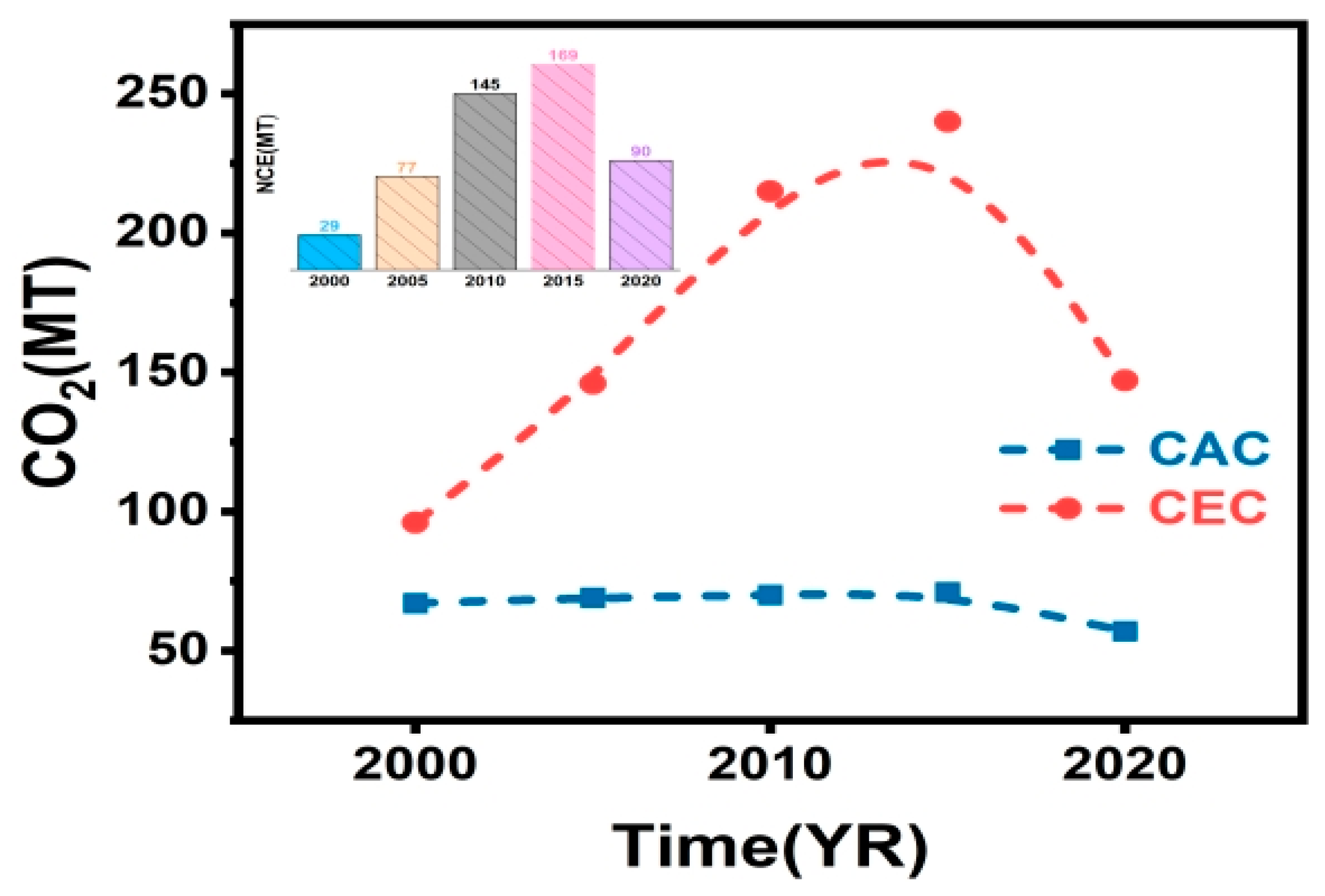
Carbon emissions at the county level in Guizhou Province exhibited a typical three-stage pattern of “growth–peak–decline” from 2000 to 2020 (Figure 2). In the first stage (2000–2005), carbon emissions increased from 0.96 × 10⁸ tons to 1.46 × 10⁸ tons, reflecting the expansion of energy demand in the early stage of industrialization. In the second stage (2005–2015), carbon emissions entered a period of rapid growth, climbing from 1.46 × 10⁸ tons to 2.4 × 10⁸ tons, driven primarily by the dual forces of a high-carbon energy structure and an increasing share of heavy industry [53].
In the third stage (2015–2020), carbon emissions declined to 1.47 × 10⁸ tons, indicating the initial effectiveness of ecological restoration and structural adjustment measures. This evolutionary trajectory differs from the national carbon emission trends, as less-developed central and western provinces emitted substantial carbon dioxide to meet the investment demands of developed eastern provinces. However, as China’s economy enters the “new normal” and economic growth transitions from investment-driven to consumption-driven, the growth rate of carbon dioxide emissions from investment demand is expected to decelerate [54]. From an interprovincial comparative perspective, the carbon emission characteristics of Guizhou are deeply constrained by its resource endowments and industrial structure. Although the share of Guizhou’s tertiary industry first exceeded 50% in 2018, it remained significantly lower than that of municipalities such as Beijing (83.8%) and Shanghai (73.1%), which have achieved strong decoupling through high-value-added industries [53]. In Southwest China, Chongqing relies on natural gas resources (accounting for 18.3% of its energy consumption), Sichuan depends on its natural gas reserves (comprising one-fifth of the national total), and Yunnan leverages its hydropower advantages. All three provinces exhibit lower carbon emission intensities than Guizhou. By contrast, Guizhou’s coal-dominated energy structure, similar to that of Shanxi [55], leads to persistently high carbon emission intensity, highlighting the transition challenges faced by resource-dependent provinces.
The carbon absorption in county-level areas of Guizhou Province exhibited fluctuating changes during the study period, with a slight overall increase but a clear trend. Between 2000 and 2015, carbon sink volume increased steadily from 0.67 × 10⁸ tons to 0.71 × 10⁸ tons, reflecting Guizhou Province’s sound ecological foundation and strong carbon sequestration capacity [56,57], with its development philosophy prioritizing ecological conservation, which was effectively implemented. From 2015 to 2020, carbon sink volume experienced a notable decline, dropping to 0.57 × 10⁸ tons—a downward trend primarily attributed to the encroachment of rapid economic development on land used for carbon sink purposes. This process diminished ecological carrying capacity and exacerbated pressures on the ecological environment [58]. From an individual county-level perspective, Weining Yi and Miao Autonomous County, Liping County, and Bozhou District emerged as the carbon sink counties/districts making the most substantial contributions to the overall carbon sink volume. These three counties/districts not only cover extensive geographical areas but also feature advantageous natural conditions and abundant ecological resources, with large areas of carbon sink land, thereby possessing strong carbon sequestration capacities.
Guizhou’s fragile ecosystems, complex topography, and unsustainable practices—such as hillside farming and excessive mining—have triggered a vicious cycle of poverty and environmental degradation [59,60], Its carbon emission reduction achievements do not rely on the technology-intensive pathways commonly adopted by coastal provinces [61]. Instead, it launched ecological restoration initiatives, including afforestation and desertification control, starting from the late 20th century [62], thereby achieving a forest coverage rate of 60% [58,63]. This “ecological industrialization” mechanism provides an innovative solution for regions with similar characteristics. When the marginal costs of emission reduction in traditional industries reach excessively high levels, monetizing ecosystem service values can create synergies between emission reduction efforts and developmental goals. Yet, caution is warranted that excessive reliance on carbon sinks may impede the deep decarbonization process in the industrial sector—a challenge already evident in regions like Hunan Province [64]. This highlights the necessity of policy design to balance short-term emission reduction gains with long-term transformative needs.
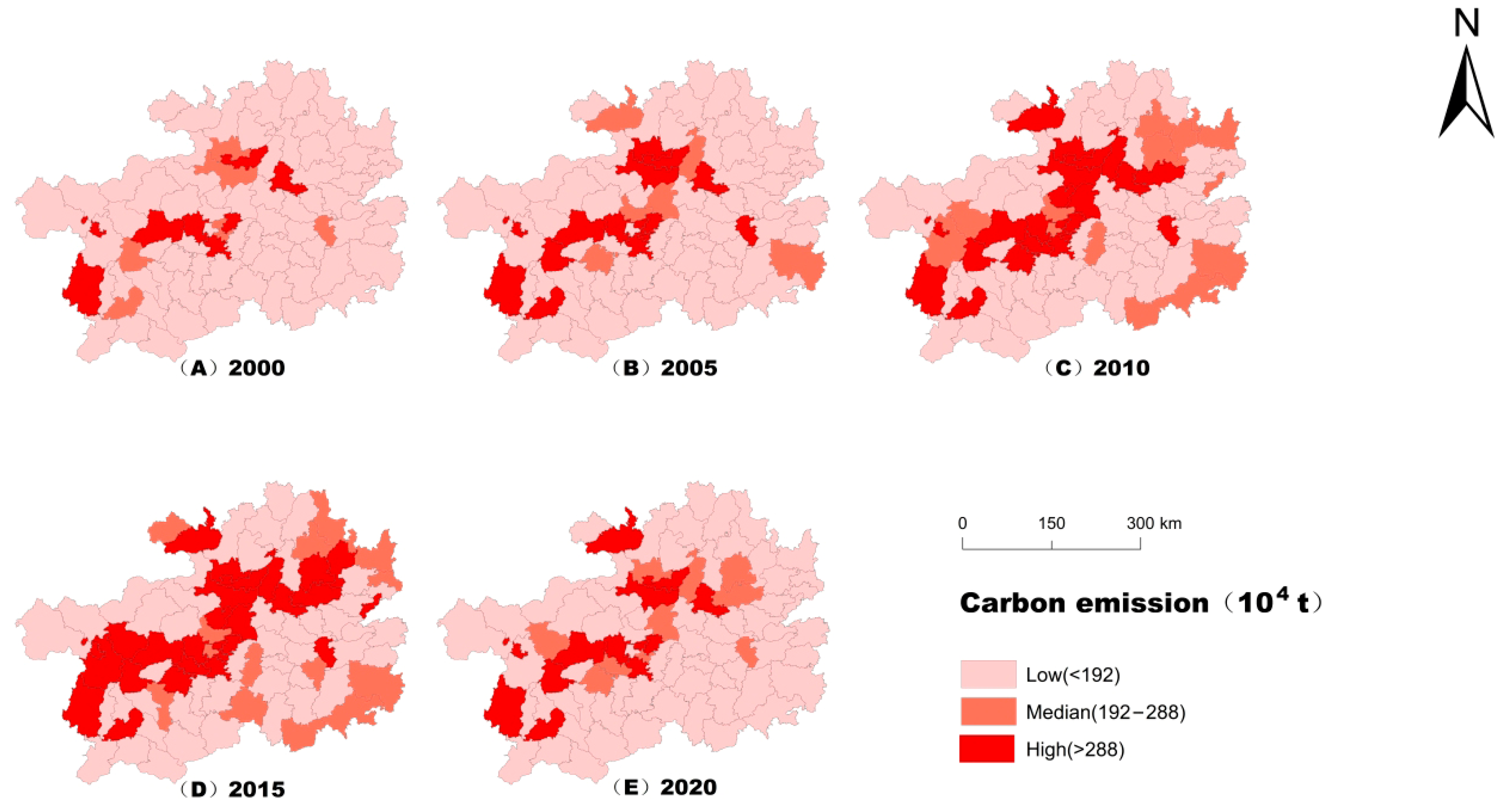
Taking the five-year average from 2000 to 2020 as the baseline period, this study establishes classification thresholds at 100% and 150% based on the statistical averages of total regional carbon emissions and carbon absorption during the baseline period [65]. Each spatial unit within the study area is then categorized into low, medium, and high grades according to its carbon emission and absorption levels relative to these thresholds. By applying spatial analysis methods and integrating with the Geographic Information System (ArcGIS) platform, this study constructs spatial distribution patterns of carbon emissions and carbon absorption and visualizes their spatial heterogeneity characteristic maps (Figure 3). The spatial patterns of carbon emissions in the study area exhibited significant dynamic evolution characteristics from 2000 to 2020. The spatial patterns of carbon emissions in Guizhou Province exhibited stage-based evolution characteristics. In 2000, there were 5 high-value zones forming a “core-dominated” pattern, while in 2005, the high-value zones expanded to 16, accompanied by the contraction of medium-value zones and spatial agglomeration effects becoming evident. From 2010 to 2015, polarization intensified as the number of high-value zones increased to 28, medium-value zones stabilized at 14, and low-value zones reduced to 46, highlighting the spatial imbalance of regional carbon emissions. By 2020, the number of high-value zones plummeted to 13, medium-value zones adjusted to 11, and low-value zones rebounded to 64. This change may reflect the implementation effects of regional industrial structure adjustment and energy conservation and emission reduction policies. The “agglomeration–diffusion” dynamic maps the trajectory of interplay between regional development policies and environmental governance.
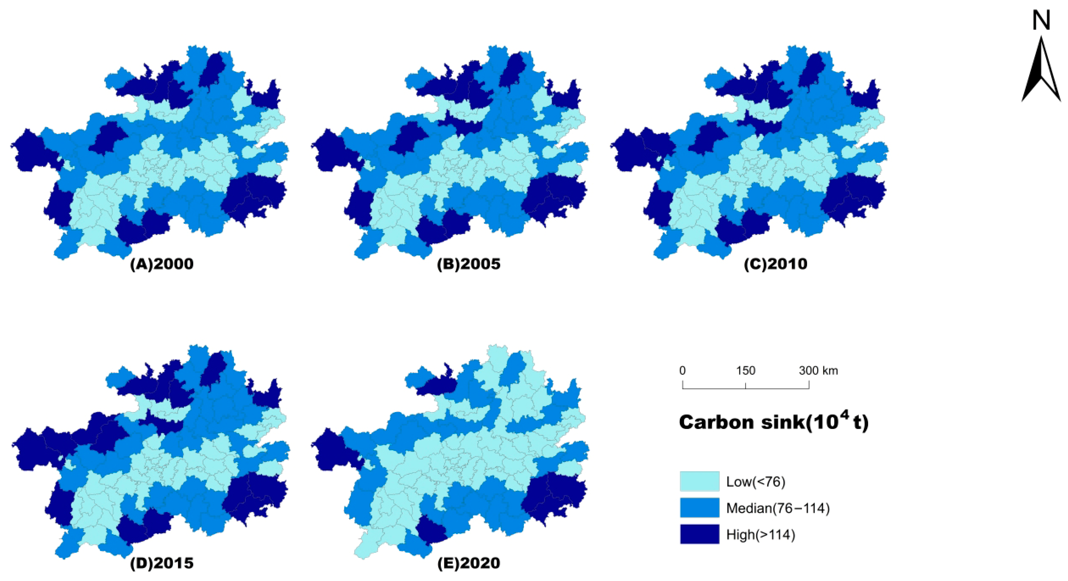
The spatial distribution of carbon absorption in county-level regions of Guizhou Province exhibits significant characteristics of spatial heterogeneity (Figure 4). High-value areas are primarily concentrated in marginal zones, forming a circular distribution pattern. Medium- and low-value areas cluster in central regions, presenting an interleaved spatial configuration.
Regarding spatial distribution patterns, regional carbon absorption demonstrates characteristics of “higher in the east, west, and south, and lower in the central and northern regions,” with the overall spatial pattern assuming a reverse “C”-shaped distribution trend. The average proportion of carbon sink capacity in high-value zones accounts for 27%, 44% in medium-value zones, and 29% in low-value zones. The regional carbon sink capacity exhibits spatial characteristics that are “higher in the middle and relatively balanced at both ends,” with medium-value zones occupying a dominant position in spatial distribution.
Guizhou Province exhibits a unique spatial pattern of carbon sources and sinks: high-value carbon storage areas are concentrated in the central and western regions, medium-value areas surround the periphery, and low-value areas are scattered, forming an overall characteristic of “a central high-value corridor with low-value zones on both eastern and western sides.” Meanwhile, high-carbon-emissions areas create a distinct corridor along the north–south axis [58]. From a national perspective, the eastern region—characterized by advanced economic development, intensive urbanization [66,67], and industrial activities—exhibits high energy consumption and relatively elevated carbon emissions. However, partial areas have enhanced carbon sinks through ecological initiatives such as increased investment in greening and afforestation. In the western region, characterized by relatively lagging economic development, the energy industry constitutes a larger proportion of the regional economy with relatively low utilization efficiency, leading to substantial carbon emissions. However, this region has vast forests and grasslands, presenting substantial carbon sink potential. Some areas have enhanced their carbon sink capabilities through measures such as afforestation and grassland conservation [68,69,70]. Compared with other provinces, the distribution of carbon sources and sinks in Fujian Province is shaped by its geographical environment and economic structures. The eastern coastal areas, characterized by robust economic development and concentrated industrial activities, demonstrate relatively high carbon emissions, while the mountainous western regions, endowed with favorable ecological conditions, exhibit comparatively higher carbon sink capacities. This province has similarities with Guizhou Province. However, the high-value carbon storage areas in central and western Guizhou are attributed to its Karst topography and abundant forest resources, while in Fujian Province, the distribution of carbon sources and sinks is influenced by the economic and ecological disparities between the eastern coastal and western inland regions [71].The county-level carbon emissions in Jiangsu Province exhibit a spatial pattern of higher values in the south and lower values in the north. The southern regions, characterized by advanced economic development, concentrated industrial activities, and dense population, show significantly higher emissions, while the northern areas maintain relatively lower emission levels [72].

4.2. Analysis of the Spatial Association Network for Carbon Budget Versus Land Use

There are notable differences in the carbon budget capacity among counties in Guizhou Province. This study employed the gravity model and social network analysis methods to explore the overall and individual spatial relationships of regional carbon budgets. Using ArcGIS10.8 software, Gephi 0.10.1, and UCINET6 tools, this study developed visualization charts for the spatial distribution of carbon budgets and their network relationships.

4.2.1. Analysis of the Spatial Association Network for Carbon Emissions

The results of this study indicate that the density of the spatial association network for carbon emissions in Guizhou Province displayed an inverted “U”-shaped pattern, increasing from 0.0075 to 0.04 before decreasing to 0.0163.
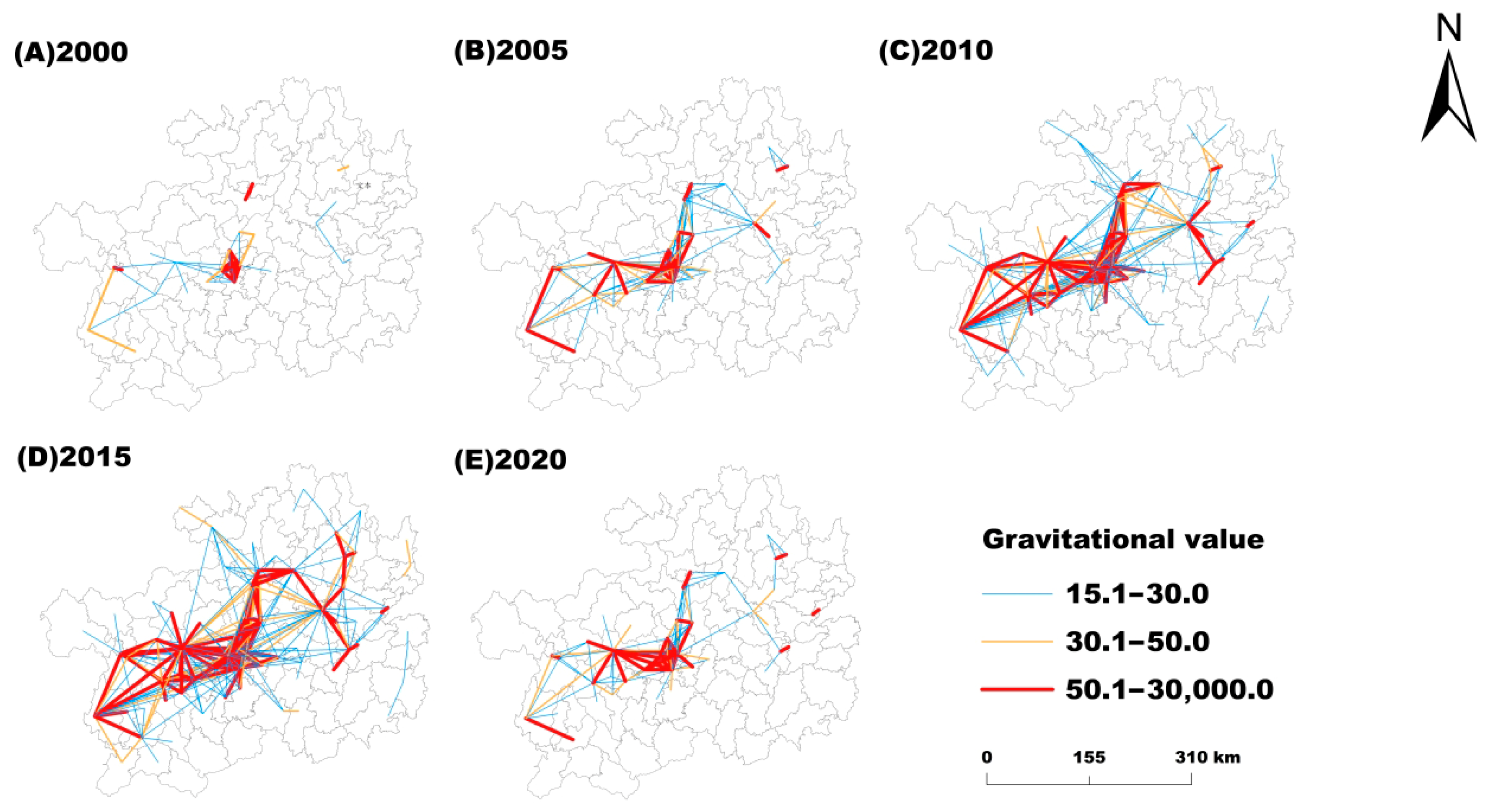
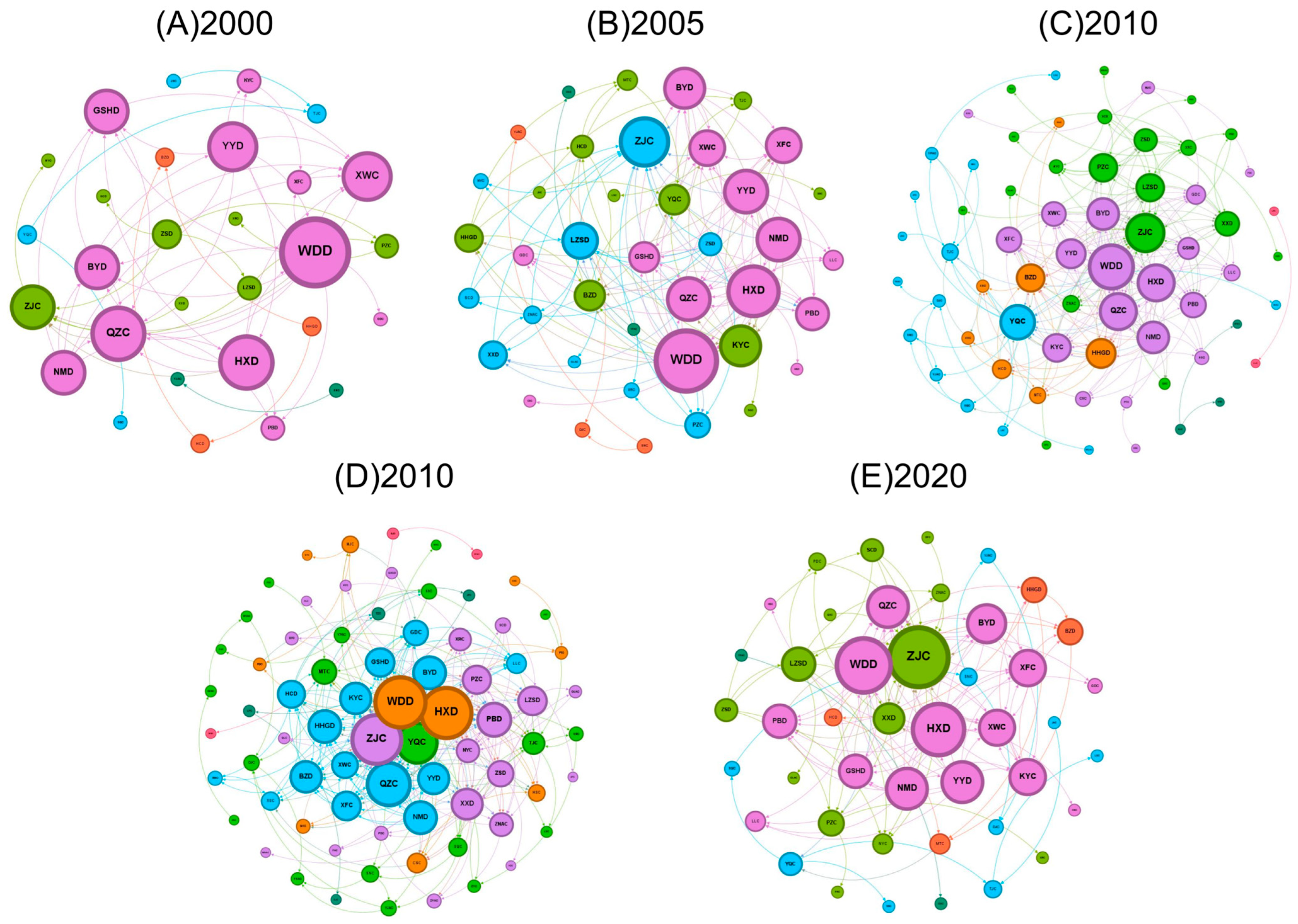
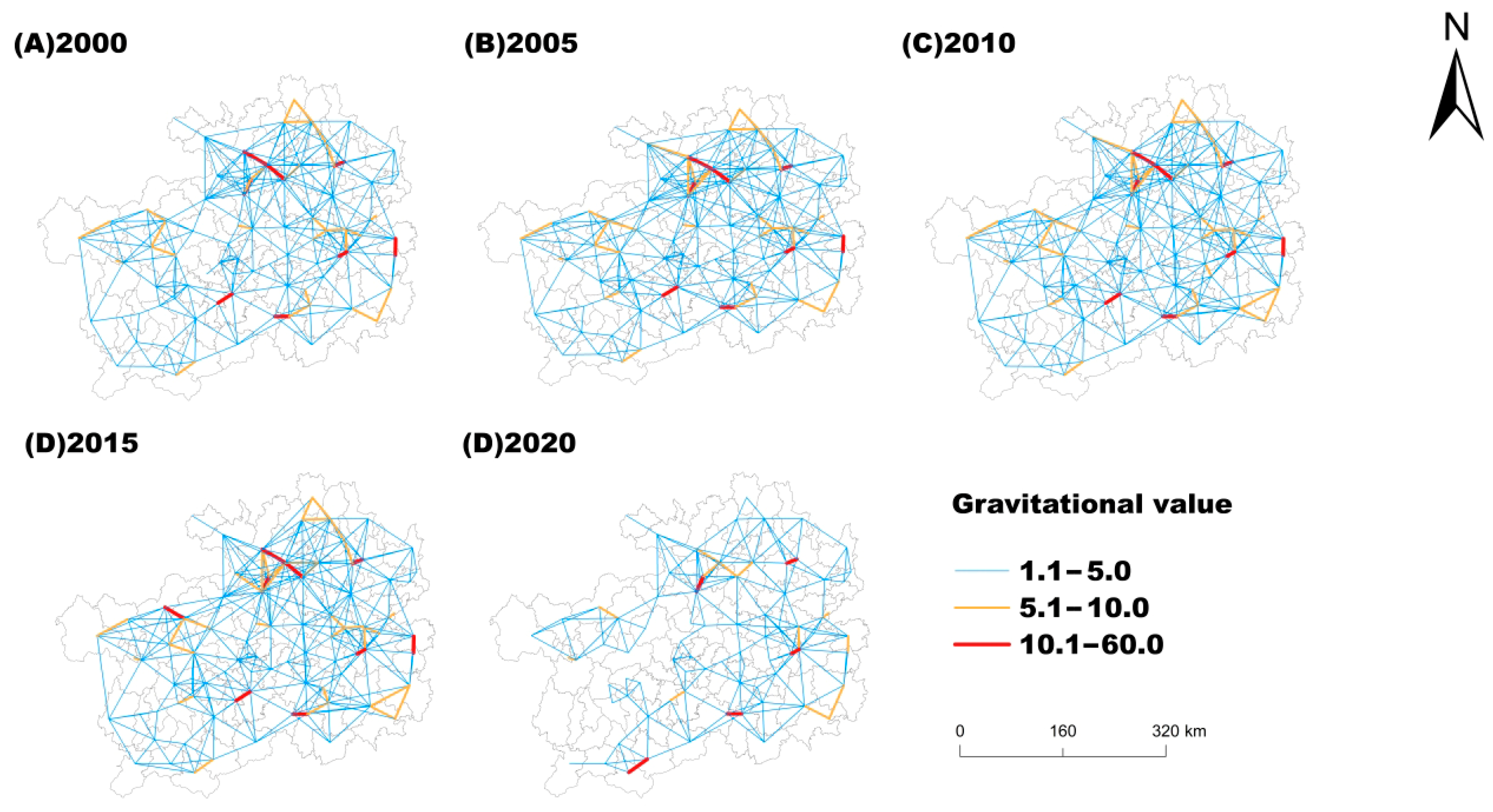
The evolution of the spatial correlation network for carbon budgets in Guizhou’s Karst counties presents a clear trajectory of spatial connections evolving from simplicity to complexity, with diffusivity characterizing this process. In 2000, the carbon emission network centered solely on Guiyang, with a limited scope of associated radiation. By 2010, a dual-core structure of Guiyang–Liupanshui gradually took shape, with significantly enhanced intensity of connection with surrounding counties; at this stage, peripheral regions (such as some counties in Qiandongnan) began to integrate into the overall association system, promoting regional spatial integration. Before 2015, the number of connecting edges in the network continued to increase (Figure 5), and the integration of peripheral counties further strengthened this spatial linkage. By 2020, the network had expanded into the Liupanshui–Guiyang–Tongren axial corridor, with core nodes distributed in a zonal pattern along major transportation routes like the Shanghai–Kunming High-Speed Railway and Hangzhou–Ruili Expressway, marking the transition of spatial correlations from local agglomeration to a complex pattern of cross-regional synergy. According to Figure 6, central districts and counties such as Wudang and Qingzhen have become core hubs due to their geographical advantages, while peripheral areas like Congjiang and Weining develop green industries based on ecological endowments with low associative intensity, forming a core–periphery dichotomous structure in the province-wide network. Data from Table A1 (Appendix A) show that betweenness centrality tells us that the top ten cities account for a cumulative contribution rate exceeding 96%, reflecting significant spatial polarization in the network. After 2015, the betweenness centrality of core hubs declined, signaling a restructuring of the network pattern—traditional hub functions weakened as new nodes emerged. High-value areas of carbon emission association are concentrated in the central and northeastern economic corridors and transportation hub zones, while low-value areas in the southwestern periphery exhibit weak intermediary functions. The network structure has undergone a process of “single-core agglomeration–multipolar differentiation–gradient restructuring,” with spatial heterogeneity strengthening as infrastructure improves.

4.2.2. Analysis of the Spatial Association Network for Carbon Absorption

Measurement results indicate that the density of the carbon absorption network in the study area exhibited an inverted “U’-shaped evolution from 2000 to 2020 (Figure 7), demonstrating synchronicity with the carbon emission network. The number of spatial connections peaked in 2015, and the connectivity of peripheral cities was superior to that of the carbon emission network. In terms of spatial structure, the most prominent feature of the network is that the connectivity of peripheral counties is significantly better than that of the carbon emission network. During the 2015 peak period, the association intensity between counties in marginal regions such as Qiandongnan and Qianxinan exceeded that of the central core area, forming a unique pattern of “dense periphery, relatively sparse center.” Among core nodes, Bozhou District, relying on its hub status in the Qianzhong Economic Zone, formed a radiation–decay association network driven by geographical proximity effects and maintained stable connections with the surrounding counties, making it the most critical “transit hub” in the network; Kaiyang County, leveraging its ecological resource advantages, maintained stable associations with surrounding counties, forming a secondary core.
According to the results presented in Figure 8, districts and counties such as Bozhou District and Kaiyang County occupy central positions in the network and serve as core nodes. Driven by the geographical proximity effect, a radiation–decay association network formed, with Bozhou District demonstrating remarkably prominent spatial location advantages as a hub of the Qianzhong Economic Zone. Data from Table A2 shows that although districts and counties with low carbon sinks, such as Qingzhen City and Renhuai City, have relatively lower carbon absorption capacities, they leverage their locational advantages to establish connections with multiple districts and counties, thus becoming intermediary hubs within the carbon absorption network. However, the intermediary role of ecologically vulnerable areas such the Yunyan District is restricted. In terms of temporal dynamics, after the betweenness centrality values peaked in 2015, the number of bridge nodes showed a downward trend, indicating a weakening tendency in cross-regional spatial connections.
The spatial networks of carbon sources/sinks in Guizhou Province exhibit distinct geographical gradient characteristics. Carbon sources form axial agglomeration along the central urbanization corridor, while carbon sink systems leverage the spatial coupling effects of ecological and economic factors to develop a multi-core networked distribution pattern. The “core–periphery” spatial polarization in urban agglomeration development is pronounced; core cities, through their economic agglomeration advantages, attract substantial resource concentration and dominate the carbon source association network—a phenomenon embodying the Matthew effect [73]. Examples include the Beijing–Tianjin–Hebei region, the Yangtze River Delta, and the Pearl River Delta [74,75,76]. Core cities consolidate their hub positions in the carbon source network through industrial radiation and factor mobility, a phenomenon also evident at the provincial scale. Taking Guizhou Province as an example, carbon sources form axial agglomerations along the central urbanization corridor, with core districts and counties emerging as key hubs via economic corridors, thus mirroring the operational mechanisms of core cities in national-level urban agglomerations. Meanwhile, the difference in the density of the carbon source network between the Guiyang Metropolitan Area and the remote regions in southwestern Guizhou highlights the decisive role of geographical location and economic foundation in shaping the carbon source network. This polarization phenomenon is equally pronounced in Shandong Province. Shandong Province’s carbon emission efficiency exhibits an “east-high–west-low” pattern [39]; eastern coastal cities such as Qingdao and Yantai, characterized by a high level of economic development, have achieved remarkable advancements in industrial structure adjustment and energy utilization efficiency, leading to relatively higher carbon emission efficiency; In contrast, western inland regions, which are relatively lagging in economic development and technological innovation, face substantial challenges in enhancing carbon emission efficiency, resulting in pronounced regional disparities. Geographical proximity effects and spatial spillover effects [77,78] play a crucial role in shaping the evolution of regional carbon source/sink networks. Taking urban agglomerations as an example, core cities, due to their geographical proximity, exert strong radiating and driving effects on surrounding cities. Through industrial transfer and technological diffusion, they promote the development of neighboring areas while simultaneously influencing the carbon source associations of these surrounding cities—an interplay that embodies the synergistic effects of geographical proximity and spatial spillover. The associations of carbon sources among cities in Shandong Province also exhibit similar characteristics [39]. With the economic development and the continuous improvement of infrastructure, the connections between cities have become increasingly close, and network density has increased. Core cities such as Jinan and Qingdao, through their geographical advantages, have become increasingly interconnected with surrounding cities. These connections not only drive the economic development of neighboring areas but also, through spatial spillover effects, exert positive impacts on surrounding cities in terms of carbon source management experience and low-carbon technologies, thereby facilitating collaborative governance of regional carbon sources and sinks. However, during the development process, as industrial structure adjustment and the spatial layout of emerging industries continue to evolve, the relationships between core cities and their surrounding areas are continually redefined, leading to a persistent transformation of the network structure. This phenomenon reflects that geographical proximity effects and spatial spillover effects are not static but instead evolve dynamically alongside regional development.

4.3. Construction’s Spatiotemporal Evolution and Analysis of Driving Factors of the Carbon Balance Spectrum in County-Level Areas of Guizhou Province

4.3.1. Construction of the Carbon Balance Spectrum for County-Level Regions in Guizhou Province

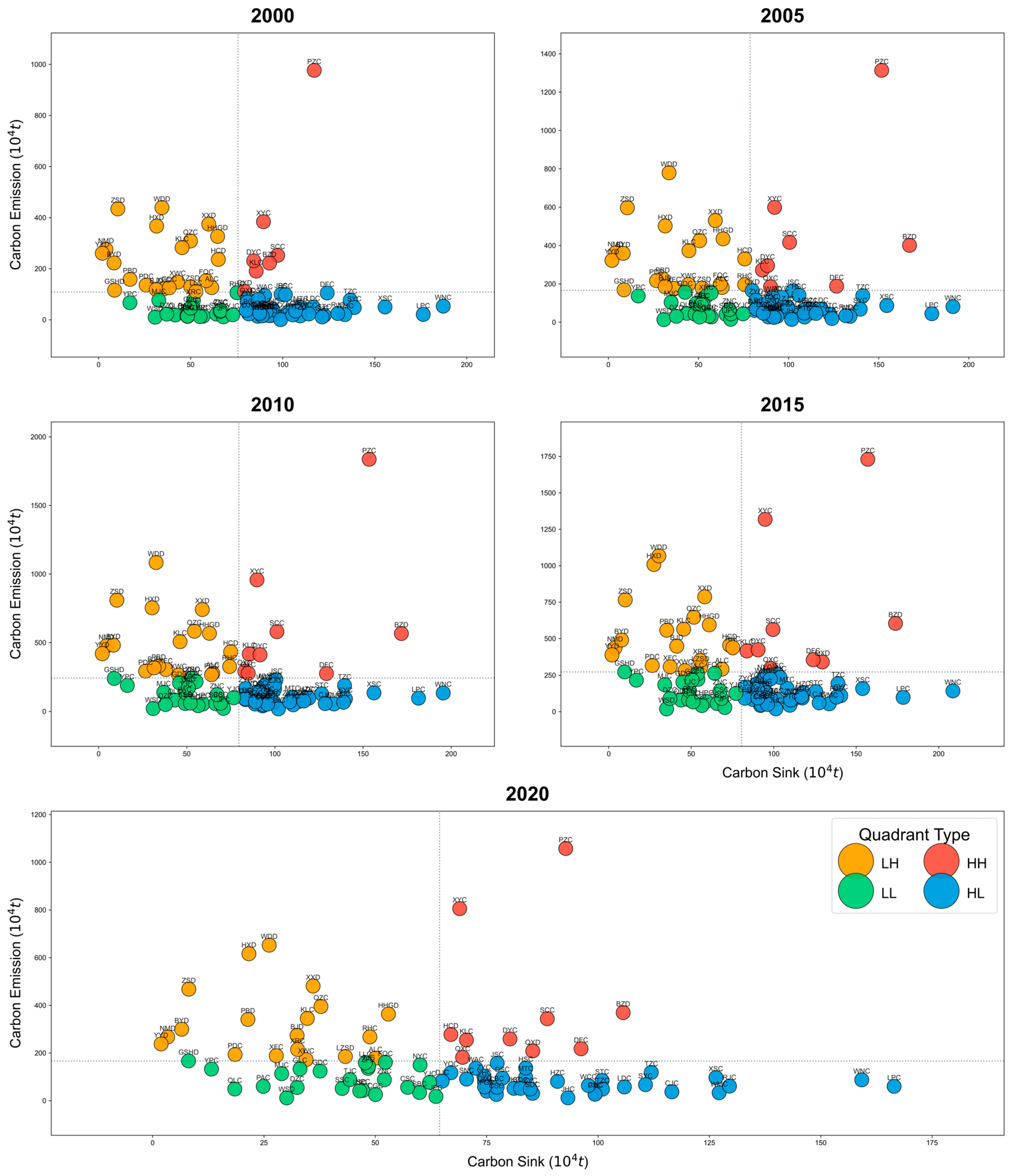
To assess regional carbon balance status, this study constructed a two-dimensional coordinate system analysis model. The model uses carbon sink volume as the horizontal axis (X-axis) and carbon emission volume as the vertical axis (Y-axis), with the average values of the two serving as the coordinate origin, as illustrated in Figure 9. Based on this coordinate system, the study area is divided into four characteristic quadrants: the first quadrant represents “high carbon sink–high carbon emission” (HH) regions, the second quadrant denotes “low carbon sink–high carbon emission” (LH) regions, the third quadrant signifies “low carbon sink–low carbon emission” (LL) regions, and the fourth quadrant defines “high carbon sink–low carbon emission” (HL) regions.
From the perspective of carbon balance, HH and LL regions exhibit relatively balanced states between carbon sources and sinks, while LH and HL regions are characterized by pronounced “carbon source dominance” and “carbon sink dominance” features respectively.
Based on the county-level panel data of Guizhou Province from 2000 to 2020, this study employed a four-quadrant classification method to deconstruct regional carbon balance patterns systematically. Spatial analysis results indicate that HH-type counties (such as Panzhou and Bozhou) exhibit characteristics of “high emissions–high carbon sequestration”; HL-type counties (e.g., Weining and Liping) demonstrate collaborative advantages of “low emissions–high carbon sink enhancement"; and LL-type counties (such as Qinglong and Wanshan) urgently need to overcome the “low economy–high ecology” development dilemma, as their GDP per unit area is only 58% of the regional average while undertaking 29% of biodiversity conservation tasks. Time-series stability analysis reveals that the conversion probability of county-level carbon metabolism types is relatively low, with ecological security patterns and industrial policy path dependence constituting the primary locking mechanisms. This study innovatively proposes differentiated transformation paths: constructing a “forestry carbon sink and clean industry” dual-drive model for HH-type areas, improving ecological product value conversion mechanisms for HL-type areas, and implementing an “ecological foundation-building and industrial empowerment” development strategy for LL-type regions. Time-series stability analysis reveals that the conversion probability of county-level carbon metabolism types is relatively low, with ecological security patterns and industrial policy path dependence constituting the primary locking mechanisms.

4.3.2. Spatiotemporal Differentiation of Carbon Balance in County-Level Regions of Guizhou Province

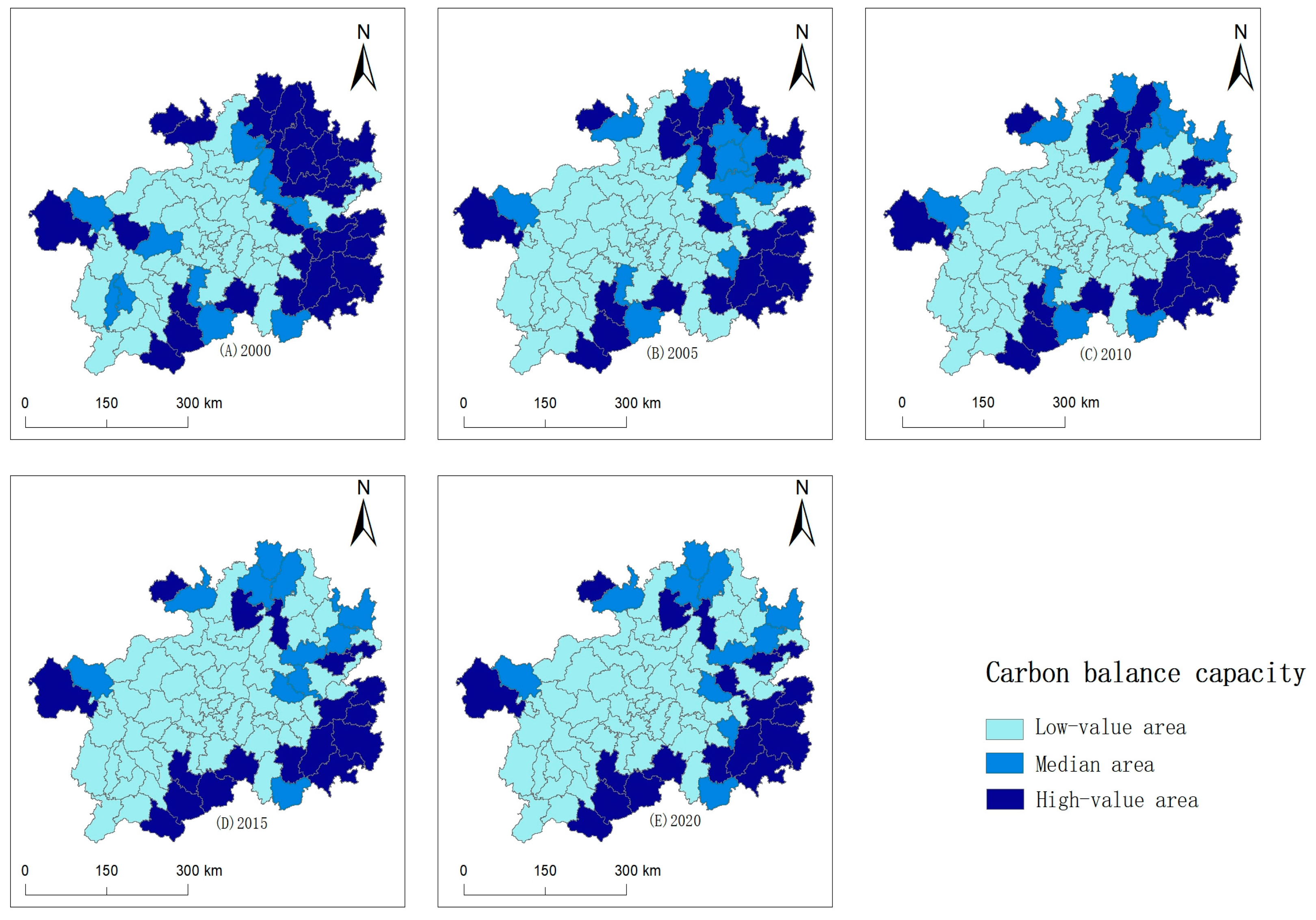
Based on the dynamic threshold classification method, this study reveals the spatiotemporal differentiation characteristics and hierarchical structural patterns of carbon balance capabilities in county-level regions of Guizhou Province. Spatial pattern analysis (Figure 10) reveals significant spatial heterogeneity in the carbon balance capacity of the study area, with low-value, medium-value, and high-value zones accounting for 58%, 17%, and 25%, respectively, forming a typical “pyramidal” hierarchical structure of ecological carrying capacity. Temporal evolution analysis indicates that the carbon balance capacity of high-value zones has remained relatively stable, underscoring the sustainability of environmental barrier functions; medium-value zones exhibit a steady upward trend, reflecting the synergistic effects of environmental restoration and urbanization development; while low-value zones show significant volatility, revealing the environmental vulnerability of resource-dependent counties.
This study analyzes the spatial distribution characteristics and change trends of carbon balance capacity (CBC) in Guizhou Province from 2000 to 2020. Findings from Figure 11 reveal that the carbon balance capacity (CBC) in Guizhou Province exhibits an inverted “C”-shaped spatial pattern characterized by higher values in eastern and southern regions and lower values in central and western areas, with pronounced regional disparities. High-value zones are concentrated in the eastern and southern peripheries, typified by Jianhe County (CBC=16.5) and Liping County, which exhibit notable advantages in forest carbon sinks. Medium- and low-value zones are concentrated in central and western regions, primarily clustering around the industrial core belt in the central-west and within the Qianzhong Urban Agglomeration. Driven by industrial emissions and urbanization, these areas generally exhibit lower carbon balance capacity (CBC) values. Notably, former high-value zones in the northern region (such as Shiqian and Sinan Counties) experienced a notable decline in CBC with the advancement of industrialization, degenerating into medium-low value zones by 2020. This trend has posed challenges to the collaborative achievement of “dual-carbon” goals among cities within urban agglomerations.

4.3.3. Dynamic Analysis of Spatial Evolution of Carbon Balance Capacity in County-Level Regions of Guizhou Province

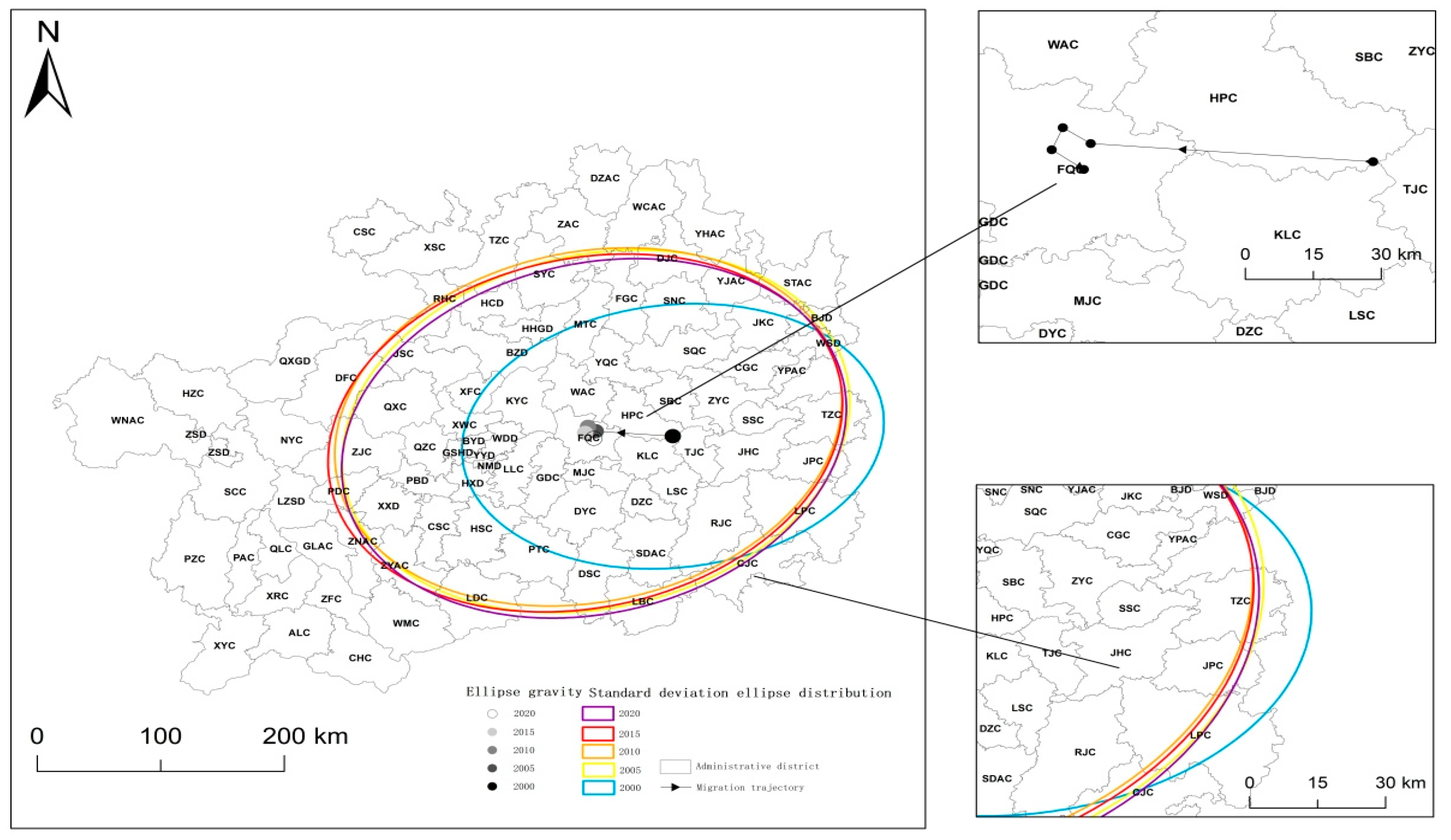
Results from Table 3 and Figure 12 indicate that the spatial distribution pattern of the study area exhibited pronounced characteristics of change between 2000 and 2020. The area of the standard deviation ellipse increased significantly from 53,081.72 km2 in 2000 to 85,343.04 km2 in 2020, with a slight decline observed during 2015–2020. This trend reveals that the spatial pattern of CBC has undergone a dynamic evolution process of first expansion and then convergence. From the perspective of elliptical axis changes, the semi-minor axis continued to increase from 109.44 km to 144.49 km. In contrast, the semi-major axis exhibited distinct phased characteristics; it increased significantly from 154.41 km to 189.01 km between 2000 and 2005, followed by a relatively stable period where it fluctuated within a narrow range of 188.02–189.01 km throughout the subsequent observation period after 2005. This indicates that the study area exhibited expansion trends in both north–south and east–west directions. The sustained higher value of the semi-major axis compared to the semi-minor axis reflects pronounced directional differentiation in the spatial distribution of the study area, with dominance in the east–west orientation and relatively limited influence in the north–south direction. The sustained higher value of the semi-major axis compared to the semi-minor axis reflects pronounced directional differentiation in the spatial distribution of the study area, with dominance in the east–west orientation and relatively limited influence in the north–south direction.
Regarding the center-of-gravity migration trajectory, the study area’s gravitational center displayed a complex movement path of “northwest–southwest–southeast” within the range of 108°6′54″ E to 107°32′26″ E in longitude and 26°46′46″ N to 26°45′44″ N in latitude, exhibiting an overall westward shift trend. This migration characteristic mutually corroborates with the changes in elliptical parameters, collectively revealing the evolutionary patterns of the study area’s spatial configuration.

4.3.4. Analysis of Driving Factors of Changes in the Carbon Balance Capacity of County-Level Regions in Guizhou Province

(1) Single-factor detection
To investigate the impact of various driving factors on the carbon balance capacity of county-level regions in Guizhou Province across different years, this study selected nine driving factors across four dimensions: natural geography and environment, economic and social development, environmental pressure and sustainability, and population and urbanization. The results of the factor impact assessment are presented in Table 4. Within the natural geography and environment dimension, NDVI (X3) dominates with consistently significant explanatory power, as its spatial heterogeneity directly reflects the promoting effect of vegetation carbon sink functions on regional carbon balance capacity [79]. High-NDVI regions establish carbon sequestration advantages through biomass accumulation. The phased driving characteristics of precipitation (X2) reflect the nonlinear regulation of carbon metabolism in Karst ecosystems by water–heat coupling processes. The economic and social development dimension exhibits significant dynamic differentiation; county-level electricity consumption (X6), with the highest explanatory power across the entire region, highlights the spatial locking effect of high-energy-consuming industries on carbon balance capacity. The rebound in its q-value after 2015 implies the resurgence risk of traditional energy dependence. Although gross regional product (X4) shows a 74.7% decline in explanatory power, it, together with the consistently high explanatory power of industrial structure (X5), collectively reveals the transformation dilemma of industrial structural rigidity in the context of decreasing returns to scale. Notably, the sharp decline in the driving effect of nighttime light (X7) confirms that the marginal impact of urban built-up area expansion on ecological resilience has reached a saturation threshold. The population and urbanization dimension exhibits typical nonlinear characteristics; the inverted U-shaped trajectory of population density (X9) indicates that moderate agglomeration reduces unit carbon emissions through infrastructure sharing, but excessive density triggers a “siphon effect” on ecological space [80], leading to the loss of elasticity in the carbon metabolism system.
(2) Interactive factor detection
Through single-factor analysis of the nine selected influencing factors, this study revealed significant differences in the effect strengths of various factors between 2000 and 2020. To investigate the joint action patterns of multiple factors, further analysis was conducted on their interactive effects (Figure 13). The results show that the interactive effects of all detected factors enhanced their explanatory power over urban carbon balance capacity, indicating that the formation of the spatial differentiation patterns of urban carbon balance capacity results from the combined effects of all factors.
Two-factor interaction detection (2000–2020) revealed that the synergistic effects of nighttime light (X7) with other indicators exhibited the strongest explanatory power, highlighting the critical role of multi-factor synergistic enhancement mechanisms in county-level carbon balance across Guizhou Province. This indicates that optimizing the spatial matching relationships between nighttime light and other driving factors represents a critical pathway through which to enhance regional carbon regulation efficiency. The explanatory power of the interactions of population density with different driving factors ranks second only to nighttime light, with population density as a secondary key driving factor. This reflects that the spatial agglomeration effects of human activities amplify carbon emission pressures through energy demand. Therefore, it is recommended to prioritize carbon reduction strategies integrating residential layout optimization and population mobility regulation in Karst landscape areas, leveraging the mitigation potential of adjusting human settlement patterns to alleviate ecological stress from concentrated energy consumption.

5. Conclusions

(1) Empirically, systematic analysis of Guizhou’s Karst counties (2000–2020) reveals striking spatiotemporal dynamics in carbon budgets: provincial carbon emissions climbed 53% (from 0.96 to 1.47 × 10⁸ t), while carbon sequestration, after peaking mid-century, declined 15% (from 0.67 to 0.57 × 10⁸ t). Spatially, emission networks shifted from single-core clustering to an axial corridor spanning Liupanshui, Guiyang, and Tongren, whereas sequestration networks retained their ecological dominance in peripheral zones. Carbon balance capacity (CBC) displayed an inverted “C"-shaped pattern—being stronger in the southeast and weaker in the central-west—with its centroid migrating westward over time. Key drivers included electricity consumption, which dominated spatial heterogeneity, and synergistic interactions between nighttime light and PM2.5, with Jianhe County maintaining peak CBC (16.5) through robust forest sinks, while Shiqian County saw steep declines due to industrial encroachment.
(2) Methodologically, this research advances carbon budget analysis in fragile ecosystems through integrated innovations. By coupling social network analysis (SNA) with gravity models, it quantifies inter-county carbon flows, moving beyond traditional reliance on geographic proximity to capture complex network interactions. Integrating geospatial detectors with standard deviational ellipses further unpacks nonlinear factor interactions—such as the interplay between NDVI and industrial structure—and tracks CBC’s spatial evolution trajectories. Critically, the study develops a county-level “carbon accounting–network analysis–driving factor detection” framework, leveraging spatial interpolation and remote sensing inversion to overcome data bottlenecks in fragmented Karst regions. These tools collectively provide a transdisciplinary lens for scaling carbon dynamics from local to regional scales.
(3) Policy implications, rooted in these findings and methods, emphasize differentiated governance and cross-regional synergy. For high-emission–high-sink (HH) regions like Panzhou, a “forestry carbon sink + clean industry” model can balance industrial activity with ecological capacity; in high-sink–low-emission (HL) areas such as Weining, enhancing ecological product value conversion mechanisms can unlock sink potential. Low-sink–low-emission (LL) regions like Qinglong may benefit from “ecological restoration + industrial upgrading” strategies. Cross-regionally, establishing a carbon-trading mechanism along the Liupanshui–Guiyang–Tongren corridor can align emission reductions with sink protection. Targeting key drivers, i.e., regulating electricity-intensive industries, optimizing nighttime light-PM2.5 synergies, and safeguarding forest ecosystems in high-CBC zones like Jianhe, will further stabilize carbon balance in this ecologically vulnerable region.
The present study has certain limitations. Spatial interpolation and inversion for county-level carbon accounting carry inherent uncertainties, as results depend on original data density and model selection, potentially biasing subsequent network analyses. Additionally, the gravity model used to quantify inter-county carbon flows relies heavily on geographical distance, potentially overlooking non-geographical drivers like industrial policies and market links, limiting network comprehensiveness. For data reliability, post-2017 county-level carbon emissions, estimated via urban growth factors, may diverge from local realities despite referencing prior studies. Cropland carbon sequestration calculations include only absorption, omitting emissions from agricultural activities, possibly understating agricultural carbon budget complexity. Moreover, findings from Guizhou’s 88 counties may not fully generalize to other Karst regions with distinct ecological and socioeconomic traits.
Future research will focus on addressing existing gaps and advancing studies on carbon cycling in Karst regions toward greater refinement and systematization. Plans involve integrating nighttime light remote sensing data with in situ observation data of Karst carbon sinks and reconstructing land-use carbon emission estimation models to enable coupled simulations of carbon emissions. Concurrently, long-term observation sites will be established in typical sample areas, and a dynamic database for carbon cycling in carbonate rock weathering will be built to support model validation. Ultimately, a carbon source–sink assessment system adapted to Karst landforms will be developed, with the aim of unraveling the specific mechanisms of carbon cycling and providing targeted theoretical and technical support for regional ecological carbon management.

Author Contributions

Writing—original draft, Writing—review and editing, Visualization, Methodology, Investigation, Supervision, Conceptualization, B.C.; Writing—original draft, Methodology, Formal analysis, Data curation, Conceptualization, J.Z.; Methodology, Investigation, Formal analysis, Data curation, Y.Y.; Methodology, Formal analysis, Data curation, W.C. All authors have read and agreed to the published version of the manuscript.

Funding

This study was funded by the National Natural Science Foundation of China (Grant No. 42462027) and the Guizhou University of Finance and Economics Innovation and Academic Emerging Scholars Project (Grant No. 2024XSXMB19).

Data Availability Statement

The original contributions presented in this study are included in the article. Further inquiries can be directed to the corresponding author.

Conflicts of Interest

The authors declare no conflicts of interest.

Appendix A

Table A1. Intermediate centrality table of carbon emissions in the middle reaches of Guizhou Province.
C/D20002005201020152020C/D20002005201020152020
NMD24.0095.50217.50414.1882.50MJC0.00 0.00 30.00 58.50 0.00
WDD18.0038.7573.6254.6561.50MTC0.00 2.50 3.33 154.27 48.00
ZJC8.0016.0044.25978.9017.00NYC0.00 0.00 0.00 0.00 0.00
PZC7.008.00196.70205.1422.00PBD0.00 0.00 8.20 60.00 0.00
HXD6.0015.6718.6741.4915.50PTC0.00 0.00 0.00 0.00 0.00
XFC2.006.1410.947.7914.00PAC0.00 0.00 0.00 0.00 0.00
XWC2.005.0056.450.732.00PDC0.00 0.00 0.00 0.00 0.00
YND1.500.000.000.000.00QXGD0.00 0.00 0.00 35.00 0.00
KYC0.5031.4215.6111.6314.00QXC0.00 0.00 0.00 0.00 2.00
ALC0.000.000.000.000.00QZC0.00 0.00 172.83 1135.82 0.00
BYD0.002.530.830.950.00QLC0.00 0.00 0.00 0.00 0.00
BJD0.000.000.000.000.00RHC0.00 0.00 0.00 0.00 0.00
BZD0.0012.7830.5452.6617.00RJC0.00 0.00 0.00 0.00 0.00
CHC0.000.000.000.000.00SSC0.00 0.00 0.00 0.00 0.00
CGC0.000.000.000.000.00SBC0.00 0.00 0.00 2.00 0.00
CSC0.000.000.000.000.00SQC0.00 0.00 2.00 10.00 45.00
CJC0.000.000.000.000.00SCD0.00 0.00 0.00 0.00 0.00
DFC0.000.000.000.500.00SNC0.00 0.00 21.00 26.71 32.00
DZC0.000.000.000.000.00STAC0.00 0.00 0.00 0.00 0.00
SYC0.000.000.000.000.00DZAC0.00 0.00 0.00 3.00 0.00
DJC0.000.0024.006.450.00TJC0.00 17.00 4.50 7.00 16.00
DYC0.000.000.000.000.00TZC0.00 0.00 0.00 0.00 0.00
DSC0.000.000.000.000.00TZC0.00 0.00 0.00 0.00 0.00
FGC0.000.000.000.000.00WSD0.00 0.00 0.00 0.00 0.00
FQC0.000.000.000.000.00GLAC0.00 0.00 0.00 0.00 0.00
WMC0.000.000.000.000.00WNAC0.00 0.00 0.00 0.00 0.00
GSHD0.000.000.000.000.00WAC0.00 0.00 0.00 0.00 0.00
GDC0.000.002.5010.500.00WCAC0.00 0.00 0.00 4.00 0.00
HZC0.000.000.000.000.00XXD0.00 3.83 12.45 43.85 11.50
HHGD0.007.0044.4788.0527.00XSC0.00 0.00 0.00 120.00 0.00
HPC0.000.000.000.000.00XRC0.00 0.00 26.00 1036.29 0.00
HCD0.002.223.4853.680.00XYC0.00 0.00 0.00 0.00 0.00
HSC0.000.000.000.000.00YHAC0.00 0.00 0.00 0.00 0.00
JHC0.000.000.000.000.00YJAC0.00 0.00 21.00 22.26 0.00
JKC0.000.000.000.000.00YQC0.00 60.00 236.17 626.90 98.00
JSC0.000.000.000.000.00YPAC0.00 0.00 40.00 74.00 0.00
JPC0.000.000.002.000.00CSC0.00 0.00 2.00 21.67 0.00
KLC0.000.000.000.000.00ZFC0.00 0.00 0.00 0.00 0.00
LSC0.000.000.000.000.00ZNAC0.00 0.00 9.00 35.39 0.00
LPC0.000.000.002.000.00ZYC0.00 0.00 0.00 0.00 0.00
LBC0.000.000.000.000.00ZAC0.00 0.00 0.00 0.00 0.00
LZTD0.0038.6722.7042.528.00ZSD0.00 0.00 43.25 108.50 0.00
LLC0.00 0.00 0.00 0.00 0.00 ZYAC0.00 0.00 0.00 0.00 0.00
LDC0.00 0.00 0.00 0.00 0.00 SDAC0.00 0.00 0.00 0.00 0.00
Table A2. Intermediate centrality table of carbon absorption in the middle reaches of Guizhou Province.
C/D20002005201020152020C/D20002005201020152020
QZC228.82 1777.05 1822.38 1815.31 244.07 ZAC45.51 49.99 44.97 45.00 10.21
BZD151.16 1758.71 1711.05 1724.03 265.59 QXC34.50 49.26 36.27 44.16 33.32
PBD214.14 1470.64 1526.54 1468.63 53.79 GLAC95.63 59.72 58.73 42.32 241.53
SDAC160.50 213.91891.09891.46659.21SNC19.21 41.78 36.97 37.12 23.32
ZYAC237.83 842.77 810.39 797.58 68.37 YJAC5.81 35.31 29.46 35.98 10.65
RJC459.01 658.93 732.56 712.43 365.82 DSC37.27 31.46 31.84 30.76 29.19
ZNAC124.46 695.64 708.18 667.93 576.11 WCAC11.17 34.58 30.23 30.55 40.17
RHC861.30 632.65 628.00 652.79 851.00 NMD127.62 31.41 33.32 30.00 86.00
WNAC77.72 363.08 352.10 502.40 1.50 CJC11.02 24.92 24.68 25.90 24.47
JHC142.36 274.18 275.78 256.06 142.31 XYC0.78 342.53 339.03 24.78 6.33
YQC177.44 237.98 233.33 226.98 279.49 GDC7.82 6.52 21.02 22.06 10.95
ZYC219.35 223.98 218.49 208.93 169.40 QLC31.53 20.14 17.35 21.08 0.00
WDD278.20 186.02 138.87 206.47 288.25 TJC27.05 20.10 18.76 19.36 39.06
LPC150.70 195.04 197.63 178.87 127.94 SSC31.14 20.69 20.06 18.79 27.22
LDC47.24 72.08 173.55 174.27 64.82 CGC19.16 18.61 18.56 17.60 13.52
SYC190.09 173.67 159.50 162.26 335.15 XFC27.44 8.46 8.14 10.20 0.00
STAC156.59 177.33 176.85 160.55 131.02 JPC16.47 10.49 10.34 8.94 11.87
XSC278.06 168.66 165.21 156.94 626.31 MJC4.73 10.57 16.71 8.25 3.56
XWC130.88 114.23 149.97 156.13 147.75 PAC0.20 6.80 6.97 7.35 4.87
WMC130.02 158.48 156.09 154.07 58.34 HCD10.35 5.30 5.15 5.84 15.80
TZC141.32 108.86 108.70 142.54 324.53 ZFC12.52 8.77 8.56 5.77 39.48
PDC488.02 182.32 173.06 139.89 554.91 NYC6.54 5.47 6.64 5.27 16.50
JKC122.55 156.06 156.59 127.80 95.97 ALC0.00 0.00 0.52 5.02 0.00
MTC130.97 134.74 133.30 119.13 164.61 DJC0.69 9.63 4.90 5.00 11.56
WAC101.33 144.86 129.92 115.33 25.45 YHAC0.29 0.28 4.70 4.80 1.13
FGC102.49 104.13 104.04 112.07 62.80 HHGD8.07 3.56 2.93 3.29 13.88
QXGD49.56 97.39 69.85 106.69 62.42 CSC4.76 2.87 4.01 2.86 13.60
DYC90.19 112.75 107.94 97.60 170.85 KLC2.28 2.57 2.25 2.20 21.51
HSC136.84 142.75 112.50 97.07 243.98 LBC1.93 3.52 1.96 1.95 7.02
SBC68.27 109.86 106.26 96.09 117.01 DZC0.00 1.35 1.38 1.37 9.41
ZJC261.46 113.98 104.58 94.63 7.50 LZSD1.00 1.31 1.31 1.14 17.50
XXD60.26 88.04 88.58 91.33 15.62 CHC1.88 1.78 0.73 0.81 6.17
SQC76.77 111.44 103.08 90.88 147.31 XRC1.48 1.03 1.03 0.70 6.33
PZC11.35 27.80 83.99 84.90 172.00 WSD3.70 2.29 2.26 0.25 4.70
JSC73.75 59.00 57.97 64.48 0.00 DZAC0.00 4.36 0.00 0.00 3.13
TZC74.11 66.03 60.79 61.53 166.11 BYD0.00 0.00 0.00 0.00 0.00
PTC105.25 65.92 68.55 60.61 17.33 BJD0.00 0.00 0.00 0.00 0.00
HPC39.51 50.68 56.49 59.35 15.67 CSC0.00 0.00 0.00 0.00 0.00
FQC63.35 67.79 57.58 53.74 56.41 GSHD0.00 0.00 0.00 0.00 0.00
SCD74.15 73.97 74.82 52.89 79.00 HZC0.00 0.00 0.00 0.00 0.00
LSC54.69 52.51 18.76 50.68 93.36 HXD0.00 0.00 33.81 0.00 0.00
KYC261.89 78.95 82.50 48.76 260.08 YPAC0.00 0.00 0.00 0.00 0.00
LLC34.21 49.08 42.46 47.80 20.99 YYD0.00 0.00 0.00 0.00 0.00
DFC47.79 44.53 72.64 47.07 132.10 ZSD0.00 0.00 0.00 0.00 0.00
Table A3. Nomenclature.
Abbreviations
SNASocial network analysis
ESCCarbon emission ecological carrying coefficient
CBCCarbon balance capacity
Variables
C l CO2 absorption quantity
L i Area of various land types
δ i Carbon sequestration rate per unit area of various land types
H c Total carbon uptake of crops
I i Carbon uptake of the i-th crop
Z i Carbon uptake rate of the i-th crop
P i Moisture content
Y i Yield
H i Economic coefficient
Y i j Intercity gravity value
D i j Distance between urban geometric centers
T Urban land use carbon budget
k Gravitational constant
y * Threshold
N Number of node counties and districts
M Carbon budget spatial correlation quantity
d i Direct association count of county i
C A Total carbon sink amount
C E Total carbon emissions
ω i Weight of each district/county
σ x Major axis
σ y Minor axis
θ Azimuth angle of ellipse
q Explanatory power of influencing factors
Table A4. Summary of functional roles of core modules.
Core ModulesSoftware
Spatiotemporal characteristics of carbon budgetOrigin 2024
Spatial association network for carbon budget in land useArcgis 10.8
Gephi 0.10.0
UCINET 6
Carbon balance spectrum for county-level regions Python 3.13

References

  1. IPPC. Asia. In Climate Change 2022–Impacts, Adaptation and Vulnerability: Working Group II Contribution to the Sixth Assessment Report of the Intergovernmental Panel on Climate Change; Cambridge University Press: Cambridge, UK, 2023; pp. 1457–1580. [Google Scholar]
  2. IPPC. Summary for Policymakers. In Climate Change 2022–Impacts, Adaptation and Vulnerability: Working Group II Contribution to the Sixth Assessment Report of the Intergovernmental Panel on Climate Change; Cambridge University Press: Cambridge, UK, 2023; pp. 3–34. [Google Scholar]
  3. Yang, Y.; Qu, S.; Cai, B.; Liang, S.; Wang, Z.; Wang, J.; Xu, M. Mapping global carbon footprint in China. Nat. Commun. 2020, 11, 2237. [Google Scholar] [CrossRef] [PubMed]
  4. Wang, Y.; Yang, H.; Sun, R. Effectiveness of China’s provincial industrial carbon emission reduction and optimization of carbon emission reduction paths in “lagging regions”: Efficiency-cost analysis. J. Environ. Manag. 2020, 275, 111221. [Google Scholar] [CrossRef] [PubMed]
  5. Zhang, Q.-Y.; Cai, B.F.; Wang, M.D.; Wang, J.X.; Xing, Y.K.; Dong, G.X.; Zhang, Z.; Mao, X.Q. City level CO2 and local air pollutants co-control performance evaluation: A case study of 113 key environmental protection cities in China. Adv. Clim. Change Res. 2022, 13, 118–130. [Google Scholar] [CrossRef]
  6. Ma, J.; Li, L.; Wang, H.; Du, Y.; Ma, J.; Zhang, X.; Wang, Z. Carbon Capture and Storage: History and the Road Ahead. Engineering 2022, 14, 33–43. [Google Scholar] [CrossRef]
  7. Chen, L.; Tan, L.; Zhao, M.; Sinha, A.; Wang, T.; Gao, Y. Karst carbon sink processes and effects: A review. Quat. Int. 2023, 652, 63–73. [Google Scholar] [CrossRef]
  8. Zhou, G.; Jia, B.; Tao, X.; Yan, H. Estimation of karst carbon sink and its contribution to CO2 emissions over a decade using remote sensing imagery. Appl. Geochem. 2020, 121, 104689. [Google Scholar] [CrossRef]
  9. Ao, Y.; Liu, X.; Zhou, X.; Ran, G.; Yang, S.; Yuan, W.; Hu, F. Differential thresholds of net ecosystem productivity in karst and non-karst regions for identifying their potential carbon sinks areas. J. Environ. Manag. 2025, 373, 123618. [Google Scholar] [CrossRef]
  10. Zhao, M.; Li, D.; Liu, Z.; Bao, Q.; Xia, F.; Yan, H.; Chen, B.; Hu, Y.; Cai, G.; Lang, R.; et al. Karst carbon sink mechanism and its contribution to carbon neutralization under land- use management. Sci. Total Environ. 2024, 937, 173381. [Google Scholar] [CrossRef]
  11. Cai, B.; Liang, S.; Zhou, J.; Wang, J.; Cao, L.; Qu, S.; Xu, M.; Yang, Z. China high resolution emission database (CHRED) with point emission sources, gridded emission data, and supplementary socioeconomic data. Resour. Conserv. Recycl. 2018, 129, 232–239. [Google Scholar] [CrossRef]
  12. Marchi, M.; Jørgensen, S.E.; Pulselli, F.M.; Marchettini, N.; Bastianoni, S. Modelling the carbon cycle of Siena Province (Tuscany, central Italy). Ecol. Model. 2012, 225, 40–60. [Google Scholar] [CrossRef]
  13. Wu, Y.; Tam, V.W.Y.; Shuai, C.; Shen, L.; Zhang, Y.; Liao, S. Decoupling China’s economic growth from carbon emissions: Empirical studies from 30 Chinese provinces (2001–2015). Sci. Total Environ. 2019, 656, 576–588. [Google Scholar] [CrossRef]
  14. Kumar, S.; Sen, R. Are larger or denser cities more emission efficient? Exploring the nexus between urban household carbon emission, population size and density. Appl. Energy 2025, 377, 124500. [Google Scholar] [CrossRef]
  15. Xu, L.; Du, H.; Zhang, X. Driving forces of carbon dioxide emissions in China’s cities: An empirical analysis based on the geodetector method. J. Clean. Prod. 2021, 287, 125169. [Google Scholar] [CrossRef]
  16. Liu, X.; Jin, X.; Luo, X.; Zhou, Y. Quantifying the spatiotemporal dynamics and impact factors of China’s county-level carbon emissions using ESTDA and spatial econometric models. J. Clean. Prod. 2023, 410, 137203. [Google Scholar] [CrossRef]
  17. Guo, L.; Zhang, X.; Zhong, J.; Wang, D.; Miao, C.; Zhao, L.; Zhou, Z.; Liao, J.; Hu, B.; Zhu, L.; et al. Construction and Application of a Regional Kilometer-Scale Carbon Source and Sink Assimilation Inversion System (CCMVS-R). Engineering 2024, 33, 263–275. [Google Scholar] [CrossRef]
  18. Guo, M.; Chen, S.; Zhang, J.; Meng, J. Environment Kuznets Curve in transport sector’s carbon emission: Evidence from China. J. Clean. Prod. 2022, 371, 133504. [Google Scholar] [CrossRef]
  19. Zhao, Q.; Fan, L.; Chen, H.; Yang, Y.; Wang, Z. Green innovation and carbon emission reduction: Empirical insights from spatial durbin and dynamic threshold models. Int. Rev. Financ. Anal. 2025, 101, 103997. [Google Scholar] [CrossRef]
  20. Wang, C.; Wang, Q.; Liu, N.; Sun, Y.; Guo, H.; Song, X. The impact of LUCC on the spatial pattern of ecological network during urbanization: A case study of Jinan City. Ecol. Indic. 2023, 155, 111004. [Google Scholar] [CrossRef]
  21. Fu, Z.; Li, R. The contributions of socioeconomic indicators to global PM2.5 based on the hybrid method of spatial econometric model and geographical and temporal weighted regression. Sci. Total Environ. 2020, 703, 135481. [Google Scholar] [CrossRef]
  22. Radmehr, R.; Henneberry, S.R.; Shayanmehr, S. Renewable Energy Consumption, CO2 Emissions, and Economic Growth Nexus: A Simultaneity Spatial Modeling Analysis of EU Countries. Struct. Change Econ. Dyn. 2021, 57, 13–27. [Google Scholar] [CrossRef]
  23. Perissi, I.; Jones, A. An Emissions Offset Strategy to Accomplish 2 °C Long-Term Mitigation Goals in the European Union. Sustainability 2024, 16, 4783. [Google Scholar] [CrossRef]
  24. Perissi, I.; Jones, A. Influence of economic decoupling in assessing carbon budget quotas for the European Union. Carbon Manag. 2023, 14, 2217423. [Google Scholar] [CrossRef]
  25. Yu, Z.; Chen, L.; Tong, H.; Chen, L.; Zhang, T.; Li, L.; Yuan, L.; Xiao, J.; Wu, R.; Bai, L.; et al. Spatial correlations of land-use carbon emissions in the Yangtze River Delta region: A perspective from social network analysis. Ecol. Indic. 2022, 142, 109147. [Google Scholar] [CrossRef]
  26. Wang, H.; Zhang, Z. Forecasting Chinese provincial carbon emissions using a novel grey prediction model considering spatial correlation. Expert Syst. Appl. 2022, 209, 118261. [Google Scholar] [CrossRef]
  27. Ye, X.; Chuai, X. Carbon sinks/sources’ spatiotemporal evolution in China and its response to built-up land expansion. J. Environ. Manag. 2022, 321, 115863. [Google Scholar] [CrossRef] [PubMed]
  28. Zhou, L.; Wu, T.; Pu, L.; Meadows, M.; Jiang, G.; Zhang, J.; Xie, X. Spatially heterogeneous relationships of PM2.5 concentrations with natural and land use factors in the Niger River Watershed, West Africa. J. Clean. Prod. 2023, 394, 136406. [Google Scholar] [CrossRef]
  29. Long, Z.; Zhang, Z.; Liang, S.; Chen, X.; Ding, B.; Wang, B.; Chen, Y.; Sun, Y.; Li, S.; Yang, T. Spatially explicit carbon emissions at the county scale. Resour. Conserv. Recycl. 2021, 173, 105706. [Google Scholar] [CrossRef]
  30. Yang, S.; Zhu, Z.; Fu, W.; Hu, S. Tele-connection of embodied carbon emissions from industries in China’s trade: A complex network analysis. J. Environ. Manag. 2024, 366, 121652. [Google Scholar] [CrossRef]
  31. Yang, S.; Li, Y.; Zhao, Y.; Lan, A.; Zhou, C.; Lu, H.; Zhou, L. Changes in vegetation ecosystem carbon sinks and their response to drought in the karst concentration distribution area of Asia. Ecol. Inform. 2024, 84, 102907. [Google Scholar] [CrossRef]
  32. You, J.; Dong, Z.; Jiang, H. Research on the spatiotemporal evolution and non-stationarity effect of urban carbon balance: Evidence from representative cities in China. Environ. Res. 2024, 252, 118802. [Google Scholar] [CrossRef]
  33. Wang, C.; Ibrahim, H.; Wu, F.; Chang, W. Spatial and temporal evolution patterns and spatial spillover effects of carbon emissions in China in the context of digital economy. J. Environ. Manag. 2025, 373, 123811. [Google Scholar] [CrossRef]
  34. Li, S.; Zhao, X.; Pu, J.; Miao, P.; Wang, Q.; Tan, K. Optimize and control territorial spatial functional areas to improve the ecological stability and total environment in karst areas of Southwest China. Land Use Policy 2021, 100, 104940. [Google Scholar] [CrossRef]
  35. Li, S. Liu, Y.; Kang, L. Spatial spillover effect of new-type urbanization on carbon emission intensity in counties around the Poyang Lake. Resour. Sci. 2022, 44, 1449–1462. [Google Scholar]
  36. Shen, X.; Yan, R.; Jiang, M. How does planting structure change affect the agricultural net carbon sink? Evidence from the Jiangsu coastal economic Belt. Ecol. Indic. 2025, 170, 112949. [Google Scholar] [CrossRef]
  37. Shen, W.; Liang, H.; Dong, L.; Ren, J.; Wang, G. Synergistic CO2 reduction effects in Chinese urban agglomerations: Perspectives from social network analysis. Sci. Total Environ. 2021, 798, 149352. [Google Scholar] [CrossRef]
  38. Huo, T.; Cao, R.; Xia, N.; Hu, X.; Cai, W.; Liu, B. Spatial correlation network structure of China’s building carbon emissions and its driving factors: A social network analysis method. J. Environ. Manag. 2022, 320, 115808. [Google Scholar] [CrossRef]
  39. Zhang, L.; Wang, H.; Guo, B.; Liu, X.; Deng, C.; Zhao, Z.; Jiang, X.; Li, Y. Characteristics and formation mechanism of carbon emission efficiency spatial correlation network: Perspective from Shandong Province. Ecol. Indic. 2025, 170, 112996. [Google Scholar] [CrossRef]
  40. Borgatti, S.P.; Mehra, A.; Brass, D.J.; Labianca, G. Network analysis in the social sciences. Science 2009, 323, 892–895. [Google Scholar] [CrossRef]
  41. Liu, S.; Xiao, Q. An empirical analysis on spatial correlation investigation of industrial carbon emissions using SNA-ICE model. Energy 2021, 224, 120183. [Google Scholar] [CrossRef]
  42. Ghosh, S.; Dinda, S.; Chatterjee, N.D.; Dutta, S.; Bera, D. Spatial-explicit carbon emission-sequestration balance estimation and evaluation of emission susceptible zones in an Eastern Himalayan city using Pressure-Sensitivity-Resilience framework: An approach towards achieving low carbon cities. J. Clean. Prod. 2022, 336, 130417. [Google Scholar] [CrossRef]
  43. Rong, T.; Qin, M.; Zhang, P.; Chang, Y.; Liu, Z.; Zhang, Z. Spatiotemporal evolution of land use carbon emissions and multi scenario simulation in the future—Based on carbon emission fair model and PLUS model. Environ. Technol. Innov. 2025, 38, 104087. [Google Scholar] [CrossRef]
  44. Xiang, W.; Gan, L.; Cai, W. Spatiotemporal evolution characteristics and spillover effects of carbon emissions from public building in China: The tertiary industry perspective. Environ. Impact Assess. Rev. 2024, 106, 107545. [Google Scholar] [CrossRef]
  45. Yang, Y.; Lu, X.; Yu, B.; Wang, Z.; Wang, L.; Lei, K.; Zuo, L.; Fan, P.; Liang, T. Exploring the environmental risks and seasonal variations of potentially toxic elements (PTEs) in fine road dust in resource-based cities based on Monte Carlo simulation, geo-detector and random forest model. J. Hazard. Mater. 2024, 473, 134708. [Google Scholar] [CrossRef]
  46. Zheng, J.; Groenigen, K.J.; Hartley, I.P.; Xue, R.; Wang, M.; Zhang, S.; Sun, T.; Yu, W.; Ma, B.; Luo, Y.; et al. Temperature sensitivity of bacterial species-level preferences of soil carbon pools. Geoderma 2025, 456, 117268. [Google Scholar] [CrossRef]
  47. Tang, S.; Tian, D.; Wang, J.; Zhang, R.; Wang, S.; Song, J.; Wan, S.; Zhang, J.; Zhang, S.; Li, Z.; et al. Synergistic effects of multiple global change drivers on terrestrial ecosystem carbon sink. Sci. Total Environ. 2024, 906, 167554. [Google Scholar] [CrossRef]
  48. Wang, T.; Mallick, K.; Verfaille, J.; Szutu, D.; Baldocchi, D. Water scarcity in semi-arid California compromises perennial alfalfa’s high yield and carbon sinking potentials. Agric. Water Manag. 2025, 308, 109284. [Google Scholar] [CrossRef]
  49. Fornaciari, M.; Muscas, D.; Rossi, F.; Filipponi, M.; Castellani, B.; Di Giuseppe, A.; Proietti, C.; Ruga, L.; Orlandi, F. CO2 Emission Compensation by Tree Species in Some Urban Green Areas. Sustainability 2024, 16, 3515. [Google Scholar] [CrossRef]
  50. Perissi, I.; Natalini, D.; Jones, A. Assessing the Emissions Related to European Households’ Expenditures and Their Impact on Achieving Carbon Neutrality. Climate 2023, 11, 203. [Google Scholar] [CrossRef]
  51. Rao, Y.; Wang, X.; Li, H. Forecasting electricity consumption in China’s Pearl River Delta urban agglomeration under the optimal economic growth path with low-carbon goals: Based on data of NPP-VIIRS-like nighttime light. Energy 2024, 294, 130970. [Google Scholar] [CrossRef]
  52. Hong, S.; Hui, E.C.; Lin, Y. Relationships between carbon emissions and urban population size and density, based on geo-urban scaling analysis: A multi-carbon source empirical study. Urban Clim. 2022, 46, 101337. [Google Scholar] [CrossRef]
  53. Jiao, L.; Yang, R.; Chen, B.; Zhang, Y. Variation, Variation, Determinants and prediction of carbon emissions in Guizhou, a new economic growth pole in southwest China. J. Clean. Prod. 2023, 417, 138049. [Google Scholar] [CrossRef]
  54. Li, Q.; Wu, S.; Lei, Y.; Li, S.; Li, L. China’s provincial CO2 emissions and interprovincial transfer caused by investment demand. Environ. Sci. Pollut. Res. 2019, 26, 312–325. [Google Scholar] [CrossRef]
  55. Wang, K.; Li, Z.; Xu, Z.; Wang, J.; Jia, M.; Wang, L.; Yue, X.; Duo, X. Evaluating and simulating the impacts of land use patterns on carbon emissions in coal resource-based regions: A case study of Shanxi province, China. J. Clean. Prod. 2024, 458, 142494. [Google Scholar] [CrossRef]
  56. Shi, N.; Xiao, N.; Wang, Q.; Han, Y.; Feng, J.; Quan, Z. Spatial Pattern of Ecosystems and the Driving Forces in the Yangtze River Economic Zone. Res. Environ. Sci. 2019, 32, 1779–1789. [Google Scholar]
  57. Xu, X.; Liu, J.; Jiao, F.; Zhang, K.; Ye, X.; Gong, H.; Lin, N.; Zou, C. Ecological engineering induced carbon sinks shifting from decreasing to increasing during 1981–2019 in China. Sci. Total Environ. 2023, 864, 161037. [Google Scholar] [CrossRef] [PubMed]
  58. Chen, R.; Fei, X.; Zhu, J.; Chen, W.; Du, H.; Huang, Y.; Shen, Y.; Zhang, Y.; Niu, A.; Xu, P. Assessing carbon storage dynamics in an ecological civilization demonstration zone amid rapid urbanization: A multi-scenario study of Guizhou Province, China. Resour. Environ. Sustain. 2025, 21, 100223. [Google Scholar] [CrossRef]
  59. Qiu, S.; Peng, J.; Zheng, H.; Xu, Z.; Meersmans, J. How can massive ecological restoration programs interplay with social-ecological systems? A review of research in the South China karst region. Sci. Total Environ. 2022, 807, 150723. [Google Scholar] [CrossRef]
  60. Zhang, J.; Zhang, P.; Liu, Y.; Lu, S.; Wu, G. An analysis of the spatiotemporal evolution and driving force of cultivated land green utilization in karst region of southwest China. J. Clean. Prod. 2024, 434, 140002. [Google Scholar] [CrossRef]
  61. Zhang, Y.; Khan, S.U.; Wang, Y. The future is digital: Can the digital economy drive marine sustainability? Exploring regional impacts on fisheries’ carbon emissions in coastal China. J. Clean. Prod. 2025, 506, 145518. [Google Scholar] [CrossRef]
  62. Tong, X.; Wang, K.; Yue, Y.; Brandt, M.; Liu, B.; Zhang, C.; Liao, C.; Fensholt, R. Quantifying the effectiveness of ecological restoration projects on long-term vegetation dynamics in the karst regions of Southwest China. Int. J. Appl. Earth Obs. Geoinf. 2017, 54, 105–113. [Google Scholar] [CrossRef]
  63. Zhu, M.; Zhou, Z.; Wu, X.; Wan, J.; Wang, J.; Zheng, J.; Liu, R.; Li, F. Prediction and spillover effects of forest expansion and management to increase carbon sinks in karst mountainous areas: A case study in Guizhou, China. Land Use Policy 2025, 151, 107491. [Google Scholar] [CrossRef]
  64. Cheng, J.; Huang, C.; Gan, X.; Peng, C.; Deng, L. Can forest carbon sequestration offset industrial CO2 emissions? A case study of Hubei Province, China. J. Clean. Prod. 2023, 426, 139147. [Google Scholar] [CrossRef]
  65. Xia, S.; Yang, Y. Examining spatio-temporal variations in carbon budget and carbon compensation zoning in Beijing-Tianjin-Hebei urban agglomeration based on major functional zones. J. Geogr. Sci. 2022, 32, 1911–1934. [Google Scholar] [CrossRef]
  66. Abou Samra, R.M. How Urban Green Spaces Shape Unequal Cooling in Rapidly Urbanizing Egypt: Insights from Landsat and GEE Analysis. Earth Syst. Environ. 2025, 9, 605–624. [Google Scholar] [CrossRef]
  67. Rossi, F.; Di Giuseppe, A.; Soomro, A.R.; Nicolini, A.; Filipponi, M.; Castellani, B. Radiative cooling improvement by retro-reflective materials. Energy Build. 2025, 336, 115597. [Google Scholar] [CrossRef]
  68. Chen, J.; Gao, M.; Cheng, S.; Hou, W.; Song, M.; Liu, X.; Liu, Y.; Shan, Y. County-level CO2 emissions and sequestration in China during 1997–2017. Sci. Data 2020, 7, 391. [Google Scholar] [CrossRef]
  69. Wang, S.; Xie, Z.; Wang, Z. The spatiotemporal pattern evolution and influencing factors of CO2 emissions at the county level of China. Acta Geogr. Sin. 2021, 76, 3103–3118. [Google Scholar]
  70. Liu, H.; Shao, M.; Ji, Y. The Spatial Pattern and Distribution Dynamic Evolution of Carbon Emissions in China: Empirical Study Based on County Carbon Emission Data. Geogr. Sci. 2021, 41, 1917–1924. [Google Scholar]
  71. Zheng, Y.; Fan, M.; Cai, Y.; Fu, M.; Yang, K.; Wei, C. Spatio-temporal pattern evolution of carbon emissions at the city-county-town scale in Fujian Province based on DMSP/OLS and NPP/VIIRS nighttime light data. J. Clean. Prod. 2024, 442, 140958. [Google Scholar] [CrossRef]
  72. Tao, B.; Wu, F.; Wang, J.; Zhu, M.; Zhang, J.; Xing, Z. County-level source-sink balance and carbon allocation of regional peak emissions: Model construction and application. Ecol. Indic. 2025, 173, 113387. [Google Scholar] [CrossRef]
  73. Zhang, H.; Wang, Q.; Zhao, Y.; Zhai, J.; Zhang, J. Possible explanations for the “Matthew effect” of rainfall in the Beijing-Tianjin-Hebei metropolitan area. J. Hydrol. 2024, 642, 131880. [Google Scholar] [CrossRef]
  74. Wang, C.; Liu, P.; Ibrahim, H.; Yuan, R. The temporal and spatial evolution of green finance and carbon emissions in the Pearl River Delta region: An analysis of impact pathways. J. Clean. Prod. 2024, 446, 141428. [Google Scholar] [CrossRef]
  75. Shen, L.; Jiang, Y.; Zhai, D.; Wang, P. Teleconnections detection of land use carbon emissions beyond geographical proximity promotes the construction of cross-city networks. Ecol. Indic. 2025, 170, 113092. [Google Scholar] [CrossRef]
  76. Chen, J.; Li, J.; Li, G.; Zhang, J. How to recognize and characterize land use-based carbon emissions within city networks in the Beijing-Tianjin-Hebei region of China. Urban Clim. 2024, 53, 101789. [Google Scholar] [CrossRef]
  77. Chen, H.; Liu, S.; Wang, J.; Wu, Z. The effect of geographic proximity on corporate tax avoidance: Evidence from China. J. Corp. Financ. 2022, 72, 102131. [Google Scholar] [CrossRef]
  78. Zhang, R.; Song, S.; Xiu, W. Does the efficiency of capital allocation have spatial carbon emission spillover effects? Int. Rev. Financ. Anal. 2025, 99, 103938. [Google Scholar] [CrossRef]
  79. Mallick, K.; Verfaillie, J.; Wang, T.; Ortiz, A.A.; Szutu, D.; Yi, K.; Kang, Y.; Shortt, R.; Hu, T.; Sulis, M.; et al. Net fluxes of broadband shortwave and photosynthetically active radiation complement NDVI and near infrared reflectance of vegetation to explain gross photosynthesis variability across ecosystems and climate. Remote Sens. Environ. 2024, 307, 114123. [Google Scholar] [CrossRef]
  80. Ren, X.; Xiong, R.; Ni, T. Spatial network characteristics of carbon balance in urban agglomerations– a case study in Beijing-Tianjin-Hebei city agglomeration. Appl. Geogr. 2024, 169, 103343. [Google Scholar] [CrossRef]
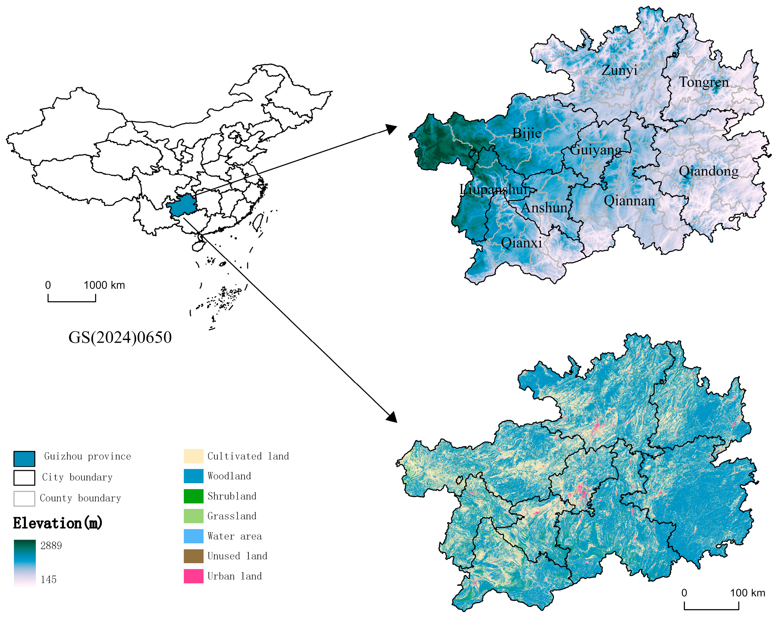
Figure 1. Study area.
Systems 13 00686 g001
Figure 2. Spatio-temporal changes in carbon emissions, carbon sequestration, and net carbon emissions from land use in Guizhou Province. (Blue: Represents the total net carbon emissions in 2000. Brown: Represents the total net carbon emissions in 2005. Grey: Represents the total net carbon emissions in 2010. Pink: Represents the total net carbon emissions in 2015. Purple: Represents the total net carbon emissions in 2020.
Systems 13 00686 g002
Figure 3. Carbon emissions changes in county-level areas of Guizhou Province from 2000 to 2020. (A) Spatial Distribution of County-Level Carbon Emissions in Guizhou Province in 2000. (B) Spatial Distribution of County-Level Carbon Emissions in Guizhou Province in 2005. (C) Spatial Distribution of County-Level Carbon Emissions in Guizhou Province in 2010. (D) Spatial Distribution of County-Level Carbon Emissions in Guizhou Province in 2015. (E) Spatial Distribution of County-Level Carbon Emissions in Guizhou Province in 2020.
Systems 13 00686 g003
Figure 4. Carbon sink changes in county-level areas of Guizhou Province from 2000 to 2020. (A) Spatial Distribution of County-Level Carbon Sinks in Guizhou Province in 2000. (B) Spatial Distribution of County-Level Carbon Sinks in Guizhou Province in 2005. (C) Spatial Distribution of County-Level Carbon Sinks in Guizhou Province in 2010. (D) Spatial Distribution of County-Level Carbon Sinks in Guizhou Province in 2015. (E) Spatial Distribution of County-Level Carbon Sinks in Guizhou Province in 2020.
Systems 13 00686 g004
Figure 5. Spatial correlation network of county-level carbon emissions in Guizhou Province from 2000 to 2020. (A) Spatial Correlation Network of County-Level Carbon Emissions in Guizhou Province in 2000. (B) Spatial Correlation Network of County-Level Carbon Emissions in Guizhou Province in 2005. (C) Spatial Correlation Network of County-Level Carbon Emissions in Guizhou Province in 2010. (D) Spatial Correlation Network of County-Level Carbon Emissions in Guizhou Province in 2015. (E) Spatial Correlation Network of County-Level Carbon Emissions in Guizhou Province in 2020.
Systems 13 00686 g005
Figure 6. Centrality map of carbon emissions by county in Guizhou Province from 2000 to 2020. (A) Centrality of County-Level Carbon Emissions in Guizhou Province in 2000. (B) Centrality of County-Level Carbon Emissions in Guizhou Province in 2005. (C) Centrality of County-Level Carbon Emissions in Guizhou Province in 2010. (D) Centrality of County-Level Carbon Emissions in Guizhou Province in 2015. (E) Centrality of County-Level Carbon Emissions in Guizhou Province in 2020.
Systems 13 00686 g006
Figure 7. The spatial correlation network of county-level carbon absorption in Guizhou Province from 2000 to 2020. (A) Spatial Correlation Network of County-Level Carbon Absorption in Guizhou Province in 2000. (B) Spatial Correlation Network of County-Level Carbon Absorption in Guizhou Province in 2005. (C) Spatial Correlation Network of County-Level Carbon Absorption in Guizhou Province in 2010. (D) Spatial Correlation Network of County-Level Carbon Absorption in Guizhou Province in 2015. (E) Spatial Correlation Network of County-Level Carbon Absorption in Guizhou Province in 2020.
Systems 13 00686 g007
Figure 8. Centrality map of carbon absorption by county in Guizhou Province from 2000 to 2020. (A) Centrality of County-Level Carbon Absorption in Guizhou Province in 2000. (B) Centrality of County-Level Carbon Absorption in Guizhou Province in 2005. (C) Centrality of County-Level Carbon Absorption in Guizhou Province in 2010. (D) Centrality of County-Level Carbon Absorption in Guizhou Province in 2015. (E) Centrality of County-Level Carbon Absorption in Guizhou Province in 2020.
Systems 13 00686 g008
Figure 9. Classification and changes in county-level carbon balance types in Guizhou Province from 2000 to 2020. (1) Classification of County-Level Carbon Balance Types in Guizhou Province in 2000. (2) Classification of County-Level Carbon Balance Types in Guizhou Province in 2005. (3) Classification of County-Level Carbon Balance Types in Guizhou Province in 2010. (4) Classification of County-Level Carbon Balance Types in Guizhou Province in 2015. (5) Classification of County-Level Carbon Balance Types in Guizhou Province in 2020.
Systems 13 00686 g009
Figure 10. Dynamic changes in the carbon balance capacity of county-level regions in Guizhou Province from 2000 to 2020. (A) Low Carbon Balance Regions at the County Level in Guizhou Province (2000–2020). (B) Medium Carbon Balance Regions at the County Level in Guizhou Province (2000–2020). (C) High Carbon Balance Regions at the County Level in Guizhou Province (2000–2020). (D) Summary Map of County-Level Carbon Balance Regions in Guizhou Province (2000–2020).
Systems 13 00686 g010
Figure 11. Spatial differentiation of carbon balance capacity of county groups in Guizhou Province from 2000 to 2020. (A) Spatial Differentiation of County-Level Carbon Balance Capacity in Guizhou Province in 2000. (B) Spatial Differentiation of County-Level Carbon Balance Capacity in Guizhou Province in 2005. (C) Spatial Differentiation of County-Level Carbon Balance Capacity in Guizhou Province in 2010. (D) Spatial Differentiation of County-Level Carbon Balance Capacity in Guizhou Province in 2015. (E) Spatial Differentiation of County-Level Carbon Balance Capacity in Guizhou Province in 2020.
Systems 13 00686 g011
Figure 12. Standard deviation ellipse distribution of carbon balance capacity and center-of-gravity migration path in the counties in Guizhou Province from 2000 to 2020.
Systems 13 00686 g012
Figure 13. Interactive detection results of factors influencing carbon balance capacity in the counties in Guizhou Province from 2000 to 2020. (A) Interaction Detection Results of Driving Factors for County-Level Carbon Balance Capacity in Guizhou Province in 2000. (B) Interaction Detection Results of Driving Factors for County-Level Carbon Balance Capacity in Guizhou Province in 2005. (C) Interaction Detection Results of Driving Factors for County-Level Carbon Balance Capacity in Guizhou Province in 2010. (D) Interaction Detection Results of Driving Factors for County-Level Carbon Balance Capacity in Guizhou Province in 2015. (E) Interaction Detection Results of Driving Factors for County-Level Carbon Balance Capacity in Guizhou Province in 2020.
Systems 13 00686 g013
Table 1. Economic coefficient, water content, and carbon absorption of crops.
Crop TypeEconomic CoefficientMoisture Content (%)Carbon Absorption Rate
Cereal crops0.4120.46
Oilseed crops0.43100.45
Cotton0.180.45
Flue-cured tobacco0.4100.45
Rapeseed0.25100.45
Beans0.34130.45
Table 3. Standard deviation ellipse parameters of carbon balance capacity in counties in Guizhou Province.
YearCentroid LongitudeCentroid DimensionSemi-major Axis/(km)Semi-Minor Axis/(km)Perimeter/(km)Area/(km2)Azimuth Angle/(°)
2000108°6′54″26°46′46″154.41109.44834.9053,081.7281.32
2005107°33′15″26°49′16″189.01145.931056.5886,645.8970.45
2010107°29′56″26°51′26″188.19144.831050.6485,620.2572.1
2015107°28′36″26°48′25″191.03144.511059.1786,717.6172.33
2020107°32′26″26°45′44″188.02144.491049.0885,343.0470.4
Table 4. Single-factor detection of spatiotemporal variation of county carbon balance coupling coordination degree in Guizhou Province.
Driving Factor20002005201020152020
qpqpqpqpqp
Temperature (X1)0.1230.080.1260.0710.0910.1970.1020.1470.1130.108
Precipitation (X2)0.0790.270.180.0135 *0.0960.1720.20.006 *0.1270.072
NDVI (X3)0.2690.000 *0.3030.000 *0.360.000 *0.250.000 *0.2620.000 *
GDP (X4)0.3230.000 *0.3540.000 *0.3890.000 *0.350.000 *0.3150.000 *
Industrial structure (X5)0.5330.000 *0.4370.000 *0.3340.000 *0.2540.000 *0.1350.063
County-level electricity consumption (X6)0.240.002 *0.2820.000 *0.2730.000 *0.2340.003 *0.2260.004 *
Nighttime lights (X7)0.7760.000 *0.6290.000 *0.6950.000 *0.5040.000 *0.5910.000 *
PM2.5 (X8)0.0990.1660.0920.1990.060.4360.0250.8450.0210.886
Population density (X9)0.3040.000 *0.430.000 *0.3850.000 *0.4780.000 *0.5120.000 *
The q-value denotes the degree to which driving factors influence carbon balance capacity; * denotes q-values that passed the significance test with p < 0.05.
Disclaimer/Publisher’s Note: The statements, opinions and data contained in all publications are solely those of the individual author(s) and contributor(s) and not of MDPI and/or the editor(s). MDPI and/or the editor(s) disclaim responsibility for any injury to people or property resulting from any ideas, methods, instructions or products referred to in the content.