Multi-Region Taxi Pick-Up Demand Prediction Based on Edge-GATv2-LSTM

Abstract

Currently, the short-term accurate prediction of multi-region taxi pick-up demand often adopts methods that integrate graph neural networks with temporal modeling. However, most models focus solely on node features during the learning process, neglecting or simplifying edge features. This study adopts a hybrid prediction framework, Edge-GATv2-LSTM, which integrates an edge-aware attention-based graph neural network (Edge-GATv2) with a temporal modeling component (LSTM). The framework not only models spatial interactions among regions via GATv2 and temporal evolution via LSTM but also incorporates edge features into the attention computation structure, jointly representing them with node features. This enables the model to perceive both node attributes and the strength of inter-regional relationships during attention weight calculation. Experiments are conducted based on real-world taxi order data from Ningbo City, and the results demonstrate that the adopted Edge-GATv2-LSTM model exhibits favorable performance in terms of pick-up demand prediction accuracy. Specifically, the model achieves the lowest RMSE and MAE of 3.85 and 2.86, respectively, outperforming all baseline methods and confirming its effectiveness in capturing spatiotemporal demand patterns. This research can provide decision-making support for taxi drivers, platform operators, and traffic management departments—for example, by offering a reference basis for optimizing taxi pick-up route planning when vehicles are unoccupied.

1. Introduction

With the increasing complexity of urban transportation systems and the continuous evolution of travel demand structures, taxi pick-up demand prediction plays a vital role in optimizing fleet dispatch and providing route recommendations for improving passenger pick-up efficiency. The significantly improved accessibility of large-scale, high-frequency travel data has made accurate taxi pick-up demand prediction based on data-driven methods increasingly feasible.

Traditional regression models are difficult to use to effectively characterize the nonlinear features and regional heterogeneity in taxi pick-up demand; therefore, recent studies have gradually introduced machine learning methods to improve prediction performance by utilizing richer variable structures and more flexible modeling frameworks. Liu et al. [1] developed an ensemble prediction model by combining ridge regression and random forest and incorporated weather and air quality indicators to effectively improve the accuracy and stability of taxi demand prediction in hotspot areas. Roy et al. [2] proposed a cross-city prediction framework to evaluate the spatial transferability of various machine learning models for ride-hailing demand prediction. The results showed that with knowledge transfer strategies, the models could still achieve good predictive performance in new cities. Building on this, Agarwal et al. [3] introduced a dynamic surge pricing factor and combined structural modeling with empirical simulation to quantify the substitution effect of platform price changes on taxi orders and demonstrated the value of price information in dispatch optimization. Sun et al. [4] focused on user cancelation behavior and developed a deep residual network model to reveal the critical impact of vehicle distance and user waiting time on the probability of order cancelation, improving the foresight and stability of platform dispatching. At the system level, Beojon et al. [5] developed a multi-region dynamic Macroscopic Fundamental Diagram (MFD) model for ride-hailing and ride-sharing services, which captures the dynamic flows of vehicles and orders across regions, thereby improving overall operational efficiency and regulatory stability. Jin et al. [6] proposed an integrated prediction framework combining fuzzy clustering and reinforcement learning. The framework first identifies typical travel patterns, dynamically selects appropriate model combinations for prediction, and then employs kernel density estimation to generate prediction intervals, thereby enhancing the accuracy and stability of ride-hailing demand forecasting.

As traditional machine learning methods struggle to capture the relationships between regions, studies have gradually adopted graph convolutional networks to model the connections and influences among regions from a holistic perspective. Tang et al. [7] constructed a spatiotemporal graph convolutional network model based on multi-community partitioning. By incorporating both a geographic adjacency graph and a functional similarity graph for joint modeling, the approach improved the clustering rationality of regional partitioning and demonstrated higher stability and generalization ability in cross-region taxi pick-up demand prediction. Feng et al. [8] proposed a multi-task graph neural network that jointly models taxi pick-up demand and OD travel demand. A shared regional representation was innovatively introduced to enable information integration across different spatial hierarchies, thereby improving the overall prediction performance.

In multi-region taxi pick-up demand prediction, graph neural networks alone have difficulty modeling the temporal variation in demand. Therefore, research has gradually shifted focus toward integrating temporal modeling methods to more fully capture spatiotemporal dependencies. Ke et al. [9] constructed a multi-task model that integrates multiple graph convolutions and GRU and, for the first time, separately modeled the spatial and temporal features of different travel modes (e.g., ride-hailing, ride-sharing). A shared mechanism was used to enable information transfer across modes, improving the prediction accuracy for various service types. Ye et al. [10] proposed a coupled graph convolutional model that dynamically adjusts the connections between regions at each layer and integrates GRU to handle the temporal variations. This enables the model to learn both inter-regional relationships and temporal patterns in demand, thereby enhancing its adaptability to changes in travel demand. Liu et al. [11] proposed a context-aware spatiotemporal network (CSTN), which innovatively integrates local spatial convolution, ConvLSTM-based temporal modeling, and a global correlation weighting mechanism. The model captures demand variations from three perspectives, influence from neighboring regions, historical evolution trends, and overall patterns, thereby improving its representation capacity and prediction performance. Zhao et al. [12] proposed a coupled neural network model that uses a dual-channel structure to separately process taxi and ride-hailing demand and integrates LSTM for temporal modeling. A semantic interaction mechanism is employed to enable information sharing between the two travel modes, improving the accuracy and coordination of multi-modal demand prediction. Chen et al. [13] constructed an integrated prediction framework combining GCN and LSTM and introduced a bagging learning strategy to address the data imbalance problem in order records. The approach demonstrated stronger prediction robustness in regions with sparse demand. Jin et al. [14] constructed a spatiotemporal prediction model named MSTIF-Net by integrating GCN and LSTM, which adopts a multi-branch structure to incorporate heterogeneous information such as holidays, weather, and orders, thereby enhancing the multi-factor modeling capability and prediction accuracy in ride-hailing demand forecasting. Chen et al. [15] proposed a deep spatiotemporal prediction model that integrates multi-source information. The model uses GCN to capture spatial dependencies across regions and employs an LSTM module for short-term temporal modeling. External variables such as weather and events are also introduced to enhance awareness of environmental influences, significantly improving short-term prediction accuracy and robustness. Zhong et al. [16] constructed the RF-STED model, which adopts a multi-branch structure combining ConvLSTM and GCN, and designed a residual feature extractor to enhance the reconstruction of OD graph structures within an encoder–decoder architecture, significantly improving the accuracy of short-term OD demand prediction. Liu et al. [17] proposed the H-ConvLSTM model, which combines hexagonal convolution with ConvLSTM to investigate how different combinations of spatial grids and temporal intervals (a total of 36 combinations) affect the prediction accuracy of ride-hailing departure and arrival demand. The experimental results show that the best performance is achieved with a grid size of 800 m and a time interval of 30 min and further reveal that departure and arrival demand exhibit different sensitivities to granularity changes.

Since traditional graph convolutional networks cannot distinguish the importance of adjacent edges, researchers have gradually combined graph neural networks (GNNs) with attention mechanisms to enhance the modeling of heterogeneity in adjacency relationships. Makhdomi et al. [18] proposed a passenger request prediction framework based on graph neural networks. By constructing an OD network graph and incorporating an attention mechanism, the framework assigns weights to adjacent edges, thereby achieving more accurate OD request prediction. Zhang et al. [19] proposed the DNEAT model, which integrates graph neural networks with attention mechanisms to construct a dynamic graph without relying on a fixed adjacency structure and enhances the ability to capture OD-level regional interaction relationships by simultaneously updating node and edge representations. Guo et al. [20] proposed a multi-gated deep graph network that integrates graph convolution, attention mechanisms, and multi-layer gating structures. By adaptively adjusting inter-regional connection strength via attention mechanisms and filtering key spatiotemporal information through gating units, the approach effectively improves the modeling accuracy and robustness of taxi pick-up demand. Wang et al. [21] proposed a graph neural network-based modeling approach that constructs a dynamic directed weighted graph to represent inter-regional travel relationships. By integrating multiple distinct attention mechanisms, including temporal attention, directional attention, and edge weight attention, the approach effectively captures changing trends in passenger travel behavior and improves prediction accuracy. Ai et al. [22] proposed a multi-step prediction model named PSA-DM, which uses a graph attention network (GAT) to model spatial relationships between regions and employs a self-attention structure to predict demand over multiple future time steps. It also feeds the previous step’s prediction results into subsequent steps, improving the coherence and accuracy of multi-step forecasting.

Although graph neural networks have achieved certain results by separately integrating attention mechanisms and LSTM, they still struggle to simultaneously account for spatial dependencies, the differential influence of neighboring nodes, and temporal variation characteristics. Therefore, research has further combined these three aspects to enhance the modeling capacity for complex traffic patterns. Mi et al. proposed a residual attention-based graph convolutional LSTM network, in which the graph convolution module is constructed based on GatedGCN. A residual attention mechanism and a multi-source external variable fusion structure are introduced, combined with LSTM for temporal modeling, significantly improving the accuracy and spatiotemporal generalization in taxi demand prediction [23]. Li et al. [24] proposed three hybrid deep prediction models that integrate CNN with various types of RNNs (LSTM, BiLSTM, GRU, and ConvLSTM) to jointly model spatial and temporal features. An attention mechanism is introduced to highlight key time periods, and multi-source external factors such as weather and holidays are incorporated. These approaches lead to improved accuracy and stability in short-term ride-hailing demand prediction tasks.

Although the above models have achieved certain success in extracting spatial structural features and capturing dependencies between nodes, they generally adopt static attention mechanisms, which makes it difficult to flexibly adjust weights based on structural differences among neighboring nodes, thereby limiting their predictive capability in complex traffic networks. Therefore, Brody et al. [25] proposed GATv2, which introduces a dynamic attention mechanism that enables the adaptive learning of attention weights under different contexts, significantly enhancing expressiveness and flexibility. On the official OGBN dataset (Open Graph Benchmark for Node Classification, a standard benchmark for graph neural networks proposed by the Stanford SNAP Lab in 2020), GATv2 improved the accuracy from 79.04% to 80.63% and reduced the error by more than 11% on the QM9 dataset, with them both outperforming conventional GNNs combined with attention mechanisms. Liu et al. designed GMTP by integrating GATv2 with BERT, which comprehensively outperformed existing baselines on the Porto and Beijing datasets [26].

To further enhance the performance of graph attention networks in dynamic graph construction and heterogeneous information modeling, researchers have begun to introduce edge features into the attention mechanism to strengthen the expressive power of modeling relationships between nodes. Chen et al. [27] constructed an edge embedding matrix to feed edge features and node features jointly into the attention mechanism, enabling the joint training of edges and nodes. This approach improved discriminative performance in structured tasks such as graph classification and social network modeling. Building on this, Zhao et al. proposed a dynamic edge construction module that integrates the GATv2 attention mechanism with temporal encoding to capture the evolution of sensor relationships in multivariate time series, enabling high-precision early fault detection in industrial Internet of Things (IIoT) systems [28]. Although existing studies have achieved notable progress in areas such as industrial monitoring and structured graph classification, the integration of edge features into graph attention mechanisms has not yet seen in-depth exploration or practical application in the context of spatial behavior modeling for taxi or ride-hailing pick-up demand prediction. This provides an important space for innovation in this study.

Table 1. Comparison of existing models for taxi/ride-hailing pick-up demand prediction.

Related Work	Methodology	GNN	LSTM/GRU	Multi-Dimensional Edge Features	Attention
					Static Linear	Dynamic Nonlinear
[1,2,3,4,5,6]	Machine Learning	×	×	×	×	×
[7]	GNN	✓	×	✓	×	×
[8]		✓	×	×	×	×
[9,10,11,12,13] [16,17]	GNN + LSTM/GRU	✓	✓	×	×	×
[14,15]		✓	✓	✓	×	×
[18,19,20,22]	GNN + Attention	✓	×	×	✓	×
[21]		✓	×	✓	✓	×
[23,24]	GNN + Attention + LSTM/GRU	✓	✓	✓	✓	×
This study	Edge-GATv2-LSTM	✓	✓	✓	×	✓

summarizes the commonly used components in existing research on taxi pick-up demand prediction, including the adopted methods, whether graph neural networks are introduced, whether LSTM or GRU is used for time series modeling, whether attention mechanisms are employed, and whether multi-dimensional edge features are integrated. Through a systematic review of the literature, it was found that most current models still exhibit limitations in modeling inter-regional relationships. Specifically, edge features are generally not incorporated into the computation of attention mechanisms, resulting in the insufficient utilization of edge information. In addition, the integration of graph modeling, attention mechanisms, and temporal structures remains incomplete, with most studies adopting only one or two of these components. Moreover, more expressive architectures such as GATv2 have not yet been effectively applied. In contrast, the prediction framework adopted in this study achieves innovations and improvements in the following aspects:

First, an edge feature encoder is designed to explicitly incorporate temporal similarity, spatial proximity, and POI similarity into the attention mechanism, thereby enhancing the model’s expressive capacity and predictive performance for heterogeneous graphs.

Second, GATv2 is introduced to capture heterogeneous associations between nodes and is combined with LSTM to effectively model the temporal evolution of taxi pick-up demand.

The remainder of this paper is organized as follows: Section 2 provides a detailed description of the structure of the adopted Edge-GATv2-LSTM model and the construction of multi-dimensional edge features. Section 3 presents the experimental setup, evaluation metrics, and prediction results and discusses the model’s adaptability to multi-region traffic flow. Finally, Section 4 concludes the paper and outlines future research directions.

2. Dynamic Prediction Model for Multi-Region Taxi Pick-Up Demand

2.1. Problem Definition

The modeling parameters for the taxi pick-up demand prediction task are shown in

Table A1. Relevant parameters.

Notation	Description
N	Total number of regional nodes
τ	Length of input historical observation window
dx	Dimensionality of the original node features
dh	Dimensionality of the LSTM hidden state
dk	Output dimensionality of a single attention head
K	Number of attention heads
demb	Output dimensionality of node embeddings
Inputs
$x_t^i\in R$	The order volume of region i at time t
$x_i\in R^{\tau }$	Time series formed by concatenating the observed values of node i over the past τ time steps
$X_t\in R^N$	Sequence of all regions at time step t
$\mathcal{X}\in R^{N\times \tau }$	Sequence of all nodes over the past τ time steps
${\mathcal{X}}_h\in R^{N\times T_h}$	Sequence immediately preceding the prediction time step
${\mathcal{X}}_d\in R^{N\times T_d}$	Sequence of the same time slot over the past few days
${\mathcal{X}}_w\in R^{N\times T_w}$	Sequence from the same weekday and time slot as the prediction step in previous weeks
${\mathcal{X}}^{\prime }\in R^{N\times 3\times T}$	${\mathcal{X}}_h$$, {\mathcal{X}}_d$$, {\mathcal{X}}_w$ Input tensor formed by concatenating the sequences
${\rho }_{i,j}$	Pearson correlation coefficient between the order volume time series of region i and region j
${\tilde{d}}_{i,j}$	Geographical proximity between region i and region j
$P_{i,j}$	Centered cosine similarity of POI distributions between region i and region j
$m_{i,j}\in R^3$	Multi-dimensional edge feature vector
Model parameters
$W^{(1,k)}\in R^{H\times 3}$	Edge feature transformation weights in the 1st layer, head k
$b^{(1,k)}\in R^H$	Bias vector in the 1st layer, head k
$W^{(2,k)}\in R^{1\times H}$	Edge feature transformation weights in the 2nd layer, head k
$b^{(2,k)}\in R$	Scalar bias in the 2nd layer, head k
$a^{(k)}\in R^{2d_k}$	Attention weight vector in head k
$W_a^{(k)}\in R^{d_k\times d}$	Input feature transformation matrix for attention head k
w, b	Final fully connected prediction layer parameters
Output
${\hat{y}}_{t+1}^i\in R$	Predicted value of node i at time slot t + 1
${\widehat{Y}}_{t+1}\in R^N$	Predicted values of all nodes at time slot t + 1
Intermediate variable
q	Sampling frequency
$T_p$	Prediction window size
$T_h$	${\mathcal{X}}_h$ Input length
$T_d$	${\mathcal{X}}_d$ Input length
$T_w$	${\mathcal{X}}_w$ Input length
$z_{i,j}^{(1,k)}\in R^H$	Representation of edge features after the first-layer nonlinear transformation
${\mathsf{\alpha }}_{i,j}^{(k)}\in R$	Attention score from node i to node j in head k
${\beta }_{i,j}^{(k)}\in R$	Attention weight after softmax normalization
$hea{d}_k\in R^{N\times d_k}$	Output of the k-th attention head
$h_i^{(k)}\in R^{d_k}$	Output vector of node i in the k-th attention head
$h_i\in R^{K\cdot d_k}$	Final representation of node i obtained by concatenating the outputs of K attention heads
$h_t^{(i)}\in R^{d_{emb}}$	Graph embedding of node i at time slot t
$H_t\in R^{N\times d_{\mathrm{emb}}}$	Embedding matrix of all nodes at time step t
$\mathcal{H}\in R^{\tau \times N\times d_{\mathrm{emb}}}$	Graph embedding tensor fed into the LSTM module
${\mathcal{H}}^{\prime }\in R^{B\times \tau \times N\cdot d_{\mathrm{emb}}}$	The reshaped tensor
$h_t^{{(i)}^{\prime }}\in R^{d_h}$	LSTM output of node i at time step t

.

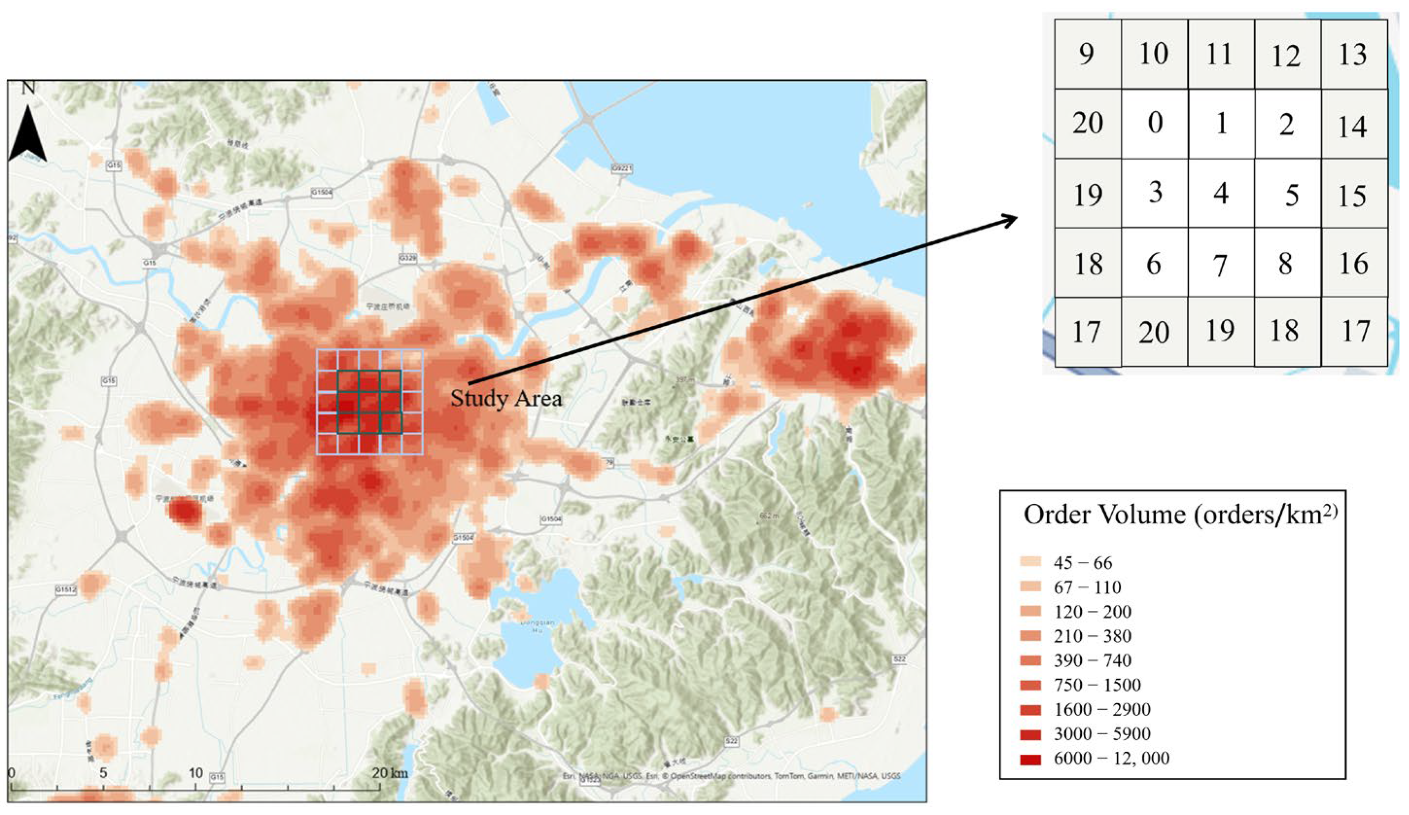
This study focuses on the region-level prediction of urban taxi pick-up demand. The study area is partitioned into N non-overlapping spatial units (1 km × 1 km), and the number of trip requests initiated in each region is counted at a fixed temporal granularity of 15 min. We model the urban regional system as an undirected graph $\mathrm{G} = (\mathrm{V}, \mathrm{E}, \mathrm{A})$, where V denotes the set of nodes, consisting of $\left|\mathrm{V}\right| = \mathrm{N}$ nodes representing spatial units; E denotes the set of edges, used to describe the connectivity between nodes; and $A\in R^{N\times N}$ is the adjacency matrix of graph G. Each node in the graph corresponds to an urban region, where a one-dimensional time series is recorded at a uniform sampling frequency, representing the number of taxi orders in that region during each time slot.

Suppose that the one-dimensional time series recorded by each node in the traffic network G represents the taxi order volume of the corresponding region. Denote the observed value of node i at time slot t as $x_t^i\in R$, which represents the number of taxi orders at that node during this time slot. Concatenate the observed values of node i over the past τ time slots to obtain a time series vector $x_i=\left(x_{t-\tau +1}^i,\dots ,x_t^i\right)\in R^{\tau }$. Denote the observed values of all nodes at time period t as $X_t={(x_t^1,x_t^2,\dots ,x_t^N)}^T\in R^N$, which represents the state of all nodes at time period t. $\mathcal{X}={\left(X_{t-\tau +1},X_{t-\tau +2},\dots ,X_t\right)}^T\in R^{N\times \tau }$ denotes the value of all the features of all the nodes over τ time slices.

2.1.1. Input Variables

Suppose the sampling frequency is q times per day. Let t denote the current time and $T_p$ be the length of the prediction window. As illustrated in Figure 1, three time series segments with lengths $T_h$, $T_d$, and $T_w$ are extracted along the temporal axis to serve as the inputs for the recent, daily periodic, and weekly periodic components, respectively. Each of $T_h$, $T_d$, and $T_w$ is assumed to be an integer multiple of $T_p$. The details of these three segments are described as follows:

• The recent segment:
  ${\mathcal{X}}_h=\left(X_{t-T_h+1},X_{t-T_h+2},\dots ,X_t\right)\in R^{N\times T_h}$, a segment of historical time series directly adjacent to the predicting period, as shown by the green part of Figure 1.
• The daily periodic segment:

  $${\mathcal{X}}_d=\left(X_{t-\left({\displaystyle \frac{T_d}{T_p}}\right)\cdot q+1},\dots ,X_{t-\left({\displaystyle \frac{T_d}{T_p}}\right)\cdot q+T_p},\hspace{0.33em}{X}_{t-\left({\displaystyle \frac{T_d}{T_p}}-1\right)\cdot q+1},\dots ,X_{t-\left({\displaystyle \frac{T_d}{T_p}}-1\right)\cdot q+T_p},\dots ,\hspace{0.33em}{X}_{t-q+1},\dots ,X_{t-q+T_p}\right)\in R^{N\times T_d}$$
  consists of the segments of the past few days at the same time period as the predicting period, as shown by the red part of Figure 1.
• The weekly periodic segment:

  $${\mathcal{X}}_w=\left(X_{t-7\cdot \left({\displaystyle \frac{T_w}{T_p}}\right)\cdot q+1},\dots ,X_{t-7\cdot \left({\displaystyle \frac{T_w}{T_p}}\right)\cdot q+T_p},\hspace{0.33em}{X}_{t-7\cdot \left({\displaystyle \frac{T_w}{T_p}}-1\right)\cdot q+1},\dots ,X_{t-7\cdot \left({\displaystyle \frac{T_w}{T_p}}-1\right)\cdot q+T_p},\dots ,\hspace{0.33em}{X}_{t-7q+1},\dots ,X_{t-7q+T_p}\right)\in R^{N\times T_w}$$
  is composed of the segments of the last few weeks, which have the same week attributes and time intervals as the forecasting period, as shown by the blue part of Figure 1.

To comprehensively model the dependencies of taxi pick-up demand across different temporal scales, we concatenate the recent segment ${\mathcal{X}}_h$, daily periodic segment ${\mathcal{X}}_d$, and weekly periodic segment ${\mathcal{X}}_w$ to form a unified input tensor ${\mathcal{X}}^{\prime }={\mathcal{X}}_h\parallel {\mathcal{X}}_d\hspace{0.33em}\parallel \hspace{0.33em}{\mathcal{X}}_w\in R^{N\times 3\times T}$. The concatenation operation merges the three segments each representing a distinct feature source into a single tensor. Each time period in the final tensor contains three feature dimensions, corresponding to recent, daily, and weekly temporal dependencies. The concatenated tensor serves as the overall input to the model, enabling the simultaneous extraction of temporal features at different time scales for predicting future taxi pick-up demand data.

Figure 1. An example of constructing the input of time series segments.

Figure 1. An example of constructing the input of time series segments.

2.1.2. Output Variables

The objective of this study is to predict the taxi pick-up demand at each node for time period t + 1 based on the given historical observation data. The predicted pick-up demand values for all nodes at time t + 1 are denoted as ${\hat{Y}}_{t+1}={({\hat{y}}_{t+1}^1,{\hat{y}}_{t+1}^2,\dots ,{\hat{y}}_{t+1}^N)}^T\in R^N$.

2.2. Overview of the Edge-GATv2-LSTM Model Architecture

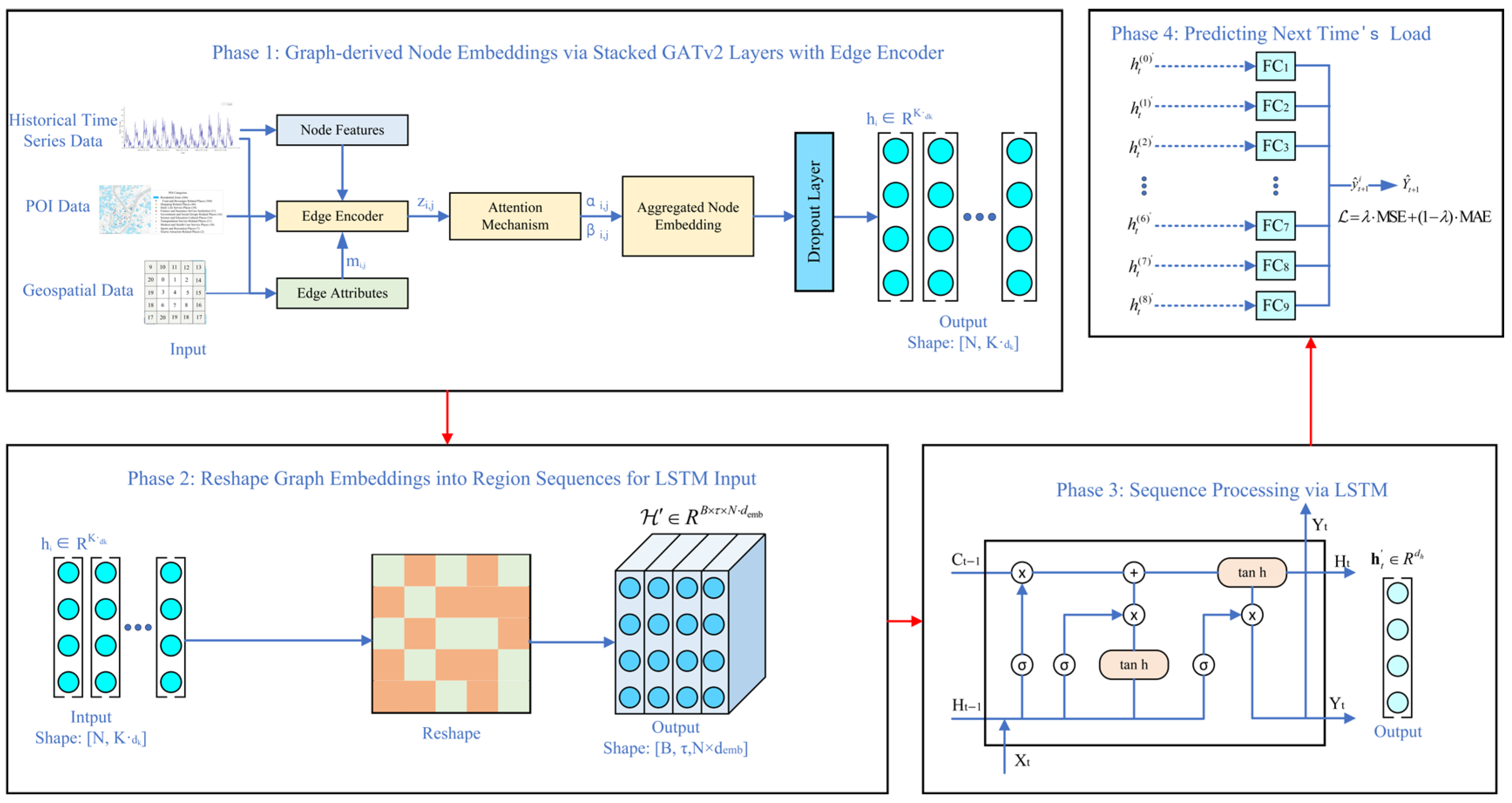
This study adopts a predictive architecture, Edge-GATv2-LSTM, which integrates graph neural networks with temporal modeling capabilities, aiming to achieve the short-term accurate forecasting of taxi pick-up demand across different urban regions. The model architecture, as illustrated in Figure 2, consists of four main stages.

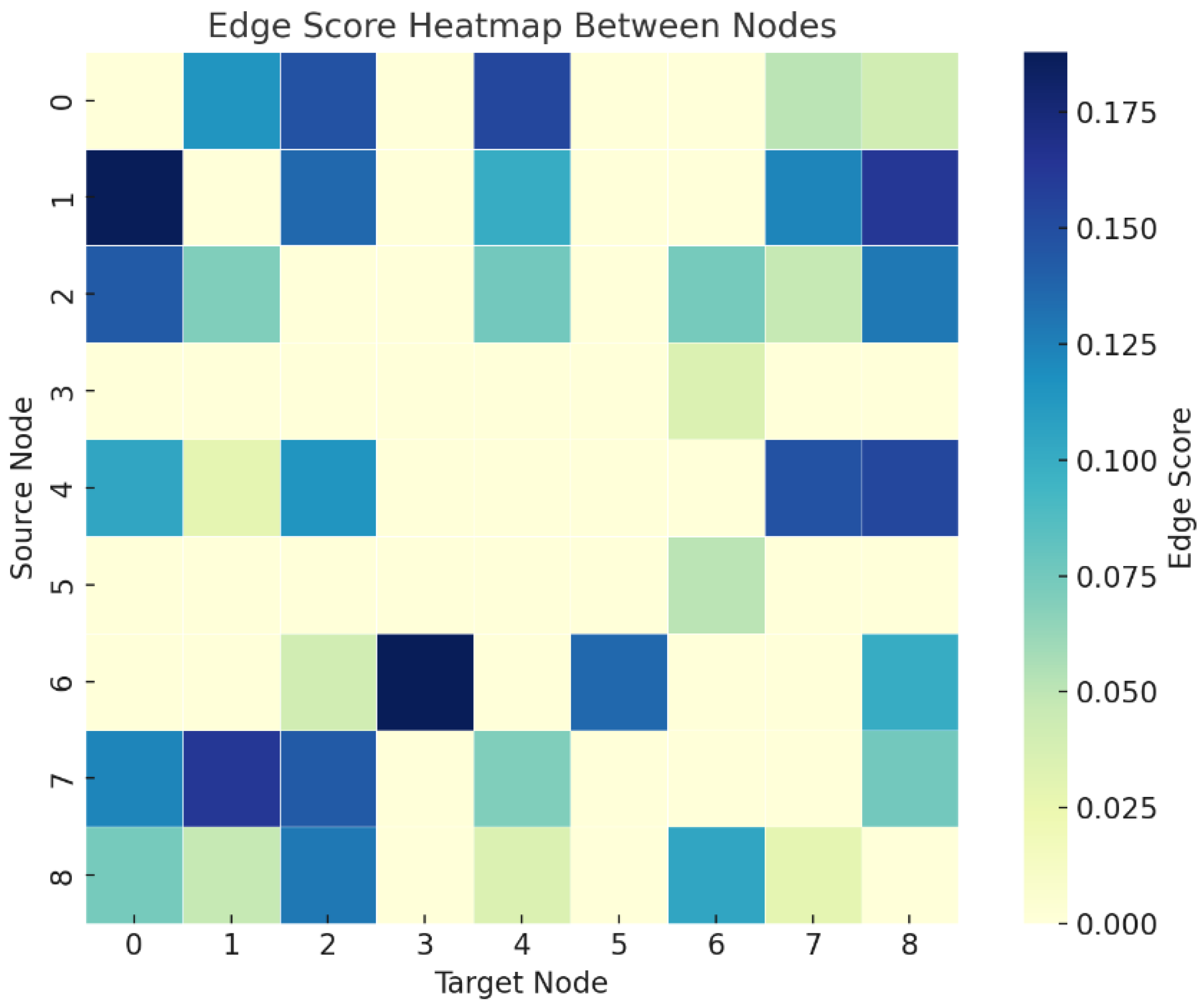
First, the urban spatial structure is modeled as an undirected graph based on the similarity of historical order behavior, and multiple types of information—such as the correlation coefficient of pick-up orders, functional similarity of regions, and geographic proximity—are incorporated as edge features. These features are embedded via an edge encoder to obtain multi-dimensional edge representations, which are then used to construct a weighted adjacency matrix. Subsequently, the GATv2 attention mechanism is introduced to adaptively model the interactions between each node and its neighbors while incorporating edge features to generate multi-head attention weights, thereby enabling the efficient modeling of heterogeneous relationships between different urban regions. A dropout mechanism is also applied to reduce the risk of overfitting, and node embedding vectors encoding spatial relationship information are ultimately generated through graph convolution operations.

Subsequently, the output of the graph neural network is reorganized into a time series format and used as the input to the LSTM network. The LSTM dynamically models the embedding sequences of different urban regions, learning the temporal patterns of taxi pick-up demand variations over time, thereby providing a temporal foundation for predicting taxi pick-up volumes.

Finally, a multi-layer fully connected network is employed to map the output of the LSTM to the predicted taxi pick-up demand for the next time period in each region. The overall prediction is optimized by jointly minimizing the weighted mean squared error (MSE) and mean absolute error (MAE) loss functions, thereby enabling the accurate prediction of future taxi pick-up demand across different regions.

2.3. Graph Structure Construction and Edge Feature Definition

2.3.1. Regional Graph Structure Construction

The adjacency matrix of the graph is generated based on the time series similarity of historical order behavior between regions. Specifically, for any two regional nodes, we extract their order volume sequences over all historical time periods in the training set and compute the Pearson correlation coefficient between the two sequences, based on which the adjacency matrix is constructed as follows:

$${[A]}_{i,j}=\left\{\begin{array}{l}1,\hspace{1em}\mathrm{if} {\rho }_{ij}\ge {\theta }_{\mathrm{corr}},\hspace{1em}i\ne j\hfill \\ 0,\hspace{1em}\mathrm{otherwise}\hfill \end{array}\right.,$$

(1)

Here, ${\rho }_{ij}={\displaystyle \frac{\mathrm{Cov}(x_i,x_j)}{\sqrt{\mathrm{Var}(x_i)\mathrm{Var}(x_j)}}}$ denotes the Pearson correlation coefficient, and ${\theta }_{\mathrm{corr}}\in [0,1]$ is the predefined correlation threshold.

2.3.2. Definition of Three-Dimensional Edge Features

To better describe the connections between different urban regions, we construct a three-dimensional edge feature vector that includes demand correlation, geographic proximity, and functional similarity. These three features have been widely used in previous research as important factors for modeling spatial relationships. Specifically, the demand correlation reflects how similar the changes in taxi orders are between two regions over time, helping to capture behavioral links; the geographic proximity describes how close two regions are in space, based on the distance between their center points, and it is commonly used in graph construction; and the functional similarity is based on the types and numbers of POIs in each region, which reflects how similar the two areas are in terms of land use and urban functions. Many studies have used these features separately or in pairs [7,8,9,10,11,12,13,14,15,16,17,18,19,20,21,22,23,24,29,30,31]. This study combines all three into a unified vector by embedding them into the GATv2 attention mechanism through a two-layer nonlinear encoder. This design enables the model to dynamically adjust attention weights based on both node attributes and edge characteristics, allowing for the more accurate modeling of inter-regional dependencies and temporal dynamics when integrated with LSTM.

To enhance the semantic representation of edges in the graph, we construct a three-dimensional edge feature vector $m_{i,j}\in R^3$ for each edge $e_{i,j}\in E$ that is determined to exist (i.e., ${[A]}_{i,j}=1$) by the adjacency matrix, as follows:

$$m_{ij}=\left[\begin{array}{c}{\rho }_{ij}\\ d_{ij}\\ P_{ij}\end{array}\right]\in R^3,$$

(2)

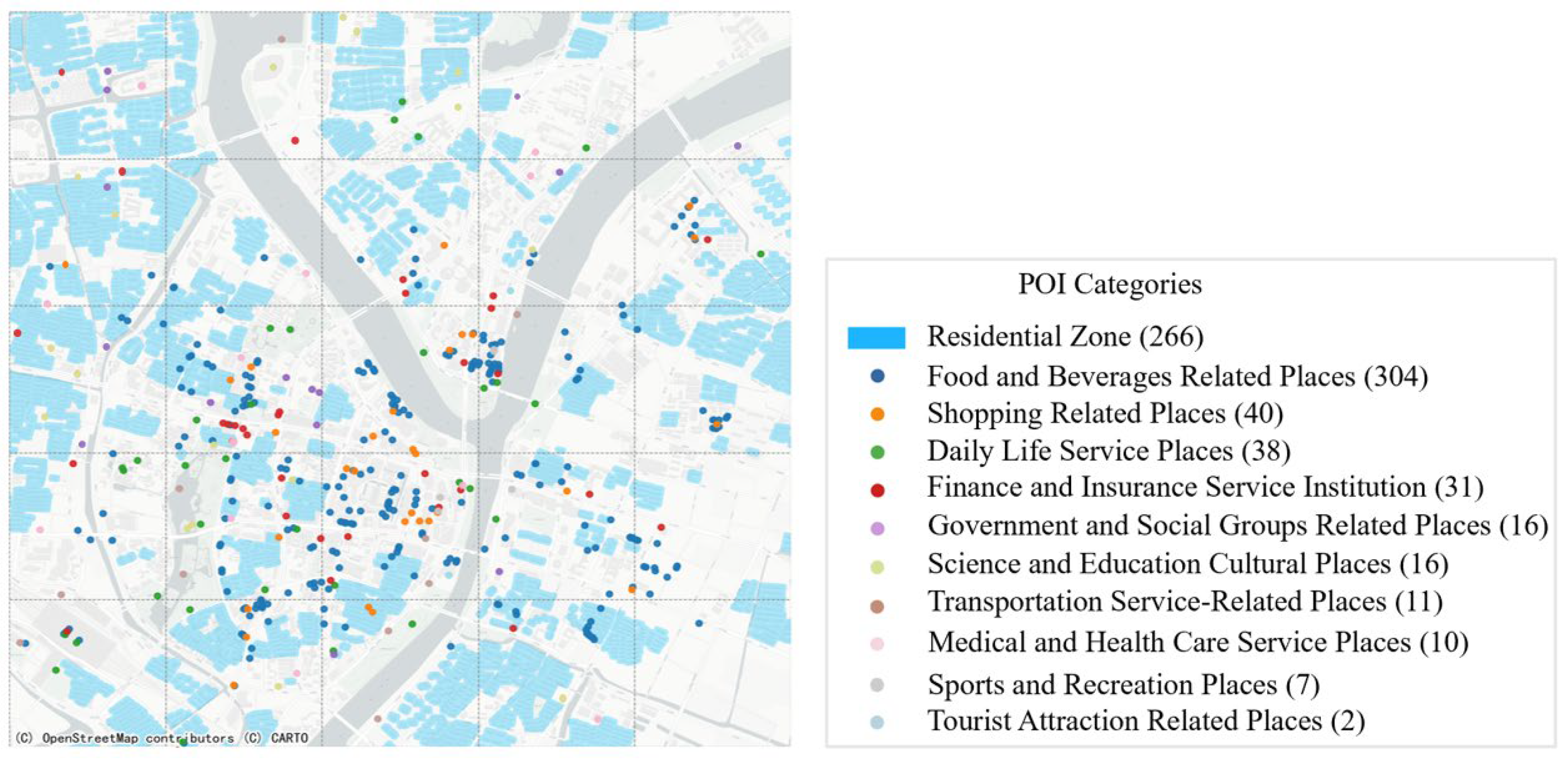
We adopt 11 types of POIs and construct a vector $P_i=\left(p_i(1),\hspace{0.33em}{p}_i(2),\hspace{0.33em}\dots ,\hspace{0.33em}{p}_i(11)\right)$, where $p_i(m)$ denotes the number of POIs of type m in region i. The functional similarity between two regions is calculated using the centered cosine similarity. The specific calculation formulas for each component are given as follows:

Geographic Proximity:

$${\tilde{d}}_{i,j}=1-{\displaystyle \frac{d_{i,j}-d_{\min }}{d_{\max }-d_{\min }}},$$

(3)

Functional Similarity:

$$P_{ij}={\displaystyle \frac{{\displaystyle \sum _{m=1}^{11}(p_i(}m)-\overline{p_i})(p_j(m)-\overline{p_j})}{\sqrt{{\displaystyle \sum _{m=1}^{11}(p_i(}m)-\overline{p_i}{)}^2}\sqrt{{\displaystyle \sum _{m=1}^{11}(}{p}_j(m)-\overline{p_j}{)}^2}}},$$

(4)

The meanings of the parameters are as follows:

${\tilde{d}}_{i,j}$: Geographic proximity (normalized distance; larger value indicates that it is closer);

$d_{i,j}$: Euclidean distance between the geographic centroids of region i and region j;

$d_{\min },\hspace{0.33em}{d}_{\max }$: Minimum and maximum geographic distances among all region pairs;

${\overline{p}}_i$: Mean number of POIs of each type in region i.

2.4. Edge-GATv2 Multi-Head Attention Network

2.4.1. Multi-Head Attention Mechanism

Prior to detailing the core components of our method, we briefly review the multi-head attention mechanism [32], which is employed in both the spatial embedding and attention modules of our model.

A multi-head self-attention mechanism uses a learned feedforward neural network to map the input sequences into three $d_k$ dimensional vectors: query vector Q, key vector µ, and value vector $\phi$. First, the scaled dot-product attention between $Q^{(k)}\in R^{N\times d_k}$ and ${\mu }^{(k)}\in R^{N\times d_k}$ is calculated, and then a softmax function is applied to obtain the attention weight α as follows:

$${\alpha }^{(k)}(Q,\mu )=\mathrm{softmax}\left({\displaystyle \frac{Q^{(k)}{\mu }^{(k)\top }}{\sqrt{d_k}}}\right),$$

(5)

where

$Q^{(k)}\in R^{N\times d_k}$ represents the query vector of the k-th attention head;

${\mu }^{(k)}\in R^{N\times d_k}$ represents the key vector of the k-th attention head;

$d_k$ denotes the dimensionality of each attention head, satisfying $d_k={\displaystyle \frac{d_{emb}}{K}}$, where d_emb is the overall output dimension of the attention mechanism and K is the number of attention heads;

${\alpha }^{(k)}\in R^{N\times N}$ represents the attention weights between all node pairs in the k-th head.

Based on the attention weights, the output of each head is computed as follows:

$$hea{d}_k={\alpha }^{(k)}(Q,\mu )\cdot {\phi }^{(k)},$$

(6)

where

${\phi }^{(k)}\in R^{N\times d_k}$: the value vector in the k-th attention head;

$hea{d}_k\in R^{N\times d_k}$: the output feature of the k-th attention head.

After computing the attention outputs from all K heads, the results are spliced together and passed through a linear transformation to obtain the final output representation:

$$MultiHead(Q,\mu ,\phi )=\left(\underset{k=1}{\overset{K}{\parallel }}hea{d}_k\right),$$

(7)

where

${\parallel }_{k=1}^{K}hea{d}_k\in R^{N\times (K\cdot d_k)}$: concatenated outputs of the K heads along the feature dimension;

$MultiHead(Q,\mu ,\phi )\in R^{N\times (K\cdot d_k)}$: the final output of the multi-head attention mechanism.

2.4.2. GATv2: An Attention Mechanism with Structural Improvements

The graph attention network (GAT) is a type of graph neural network architecture based on neighbor-weighted aggregation, originally proposed by Veličković et al. Its core idea is to treat the input features of the target node as the query and those of its neighboring nodes as keys, dynamically computing the importance scores of neighbors via an attention mechanism. These scores are then used to perform a weighted aggregation, thereby updating the node representations [33].

The query vector is generated from the features of the target node and is used to measure its degree of attention to each neighbor, while the key vector is generated from the features of the neighboring nodes and is involved in the attention scoring function. The attention score function is defined as follows:

$${\alpha }_{i,j}^{(k)}=Leaky\mathrm{Re}LU\left(a^{(k)\top }\left[W_a^{(k)}{x}_i\parallel W_a^{(k)}{x}_j\right]\right),$$

(8)

where

d: the dimensionality of the input features.

$x_i,\hspace{0.33em}{x}_j\in R^d$: the original input features of the target node i and its neighbor node j, respectively. The input feature dimension d is equal to the time window length τ, i.e., d = τ.

$d_k$: the dimensionality of each attention head.

$W_a^{(k)}\in R^{d_k\times d}$: the linear transformation matrix for the query in the k-th attention head of the attention module in GAT.

$a^{(k)}\in R^{2d_k}$: the attention weight vector in the k-th attention head of GAT.

$\parallel$: the feature concatenation operation.

LeakyReLU: a nonlinear activation function.

${\alpha }_{i,j}^{(k)}\in R$: the attention score from node iii to its neighbor node j in the k-th attention head.

However, the scoring function in GAT essentially follows a static attention mechanism, where all query nodes rank their neighbors in the same way. This prevents the model from differentiating the importance of neighbors based on the query node’s own features, thereby limiting its representational capacity.

To address the above limitation, Brody et al. proposed an improved attention mechanism called GATv2, which rearranges the computation order of the attention function. Specifically, the concatenated query and key are first passed through a nonlinear transformation, followed by scoring using an attention weight vector. This design enhances the expressive power of the model [30]. The attention scoring function is defined as follows:

$${\alpha }_{i,j}^{(k)}=a^{(k)\prime \top }Leaky\mathrm{Re}LU\left(W_a^{(k)\prime }\left[x_i\parallel x_j\right]\right),$$

(9)

where

$W_a^{(k)\prime }\in R^{d_k\times 2d}$: the linear transformation matrix in the attention module of GATv2 for the k-th attention head;

$a^{(k)\prime }\in R^{d_k}$: the attention weight vector of the k-th attention head in GATv2.

Equations (8) and (9) enable the transition from static to dynamic attention, allowing for each target node to adaptively select neighbor information based on its own state. GATv2 has demonstrated stronger generalization and robustness across various tasks and has become a mainstream alternative in graph attention modeling.

Building on the GATv2 attention mechanism, this study introduces edge feature awareness by feeding a combined input of three-dimensional edge attributes $m_{i,j}$ and node concatenation features $\left[x_i\parallel x_j\right]$ into the attention scoring function, enhancing the expressiveness of the edge information.

2.4.3. Edge-GATv2: An Improved Graph Attention Network Algorithm with Edge Weight Consideration

To transform the three-dimensional edge features into scalar weights for input into the graph attention mechanism, we design an edge feature encoder consisting of a two-layer feedforward network. Let H denote the hidden dimension, which is used to map the initial three-dimensional edge features into an H-dimensional nonlinear vector representation, in order to enhance the representational capacity of the edge information.

$$z_{i,j}^{(1,k)}=ELU\left(W^{(1,k)}{m}_{i,j}+b^{(1,k)}\right),$$

(10)

$$l_{i,j}^{(k)}=W^{(2,k)}{z}_{i,j}^{(1,k)}+b^{(2,k)},$$

(11)

where

$W^{(1,k)}\in R^{H\times 3},\hspace{1em}{b}^{(1,k)}\in R^H$: the first-layer linear transformation parameters for the k-th attention head;

$W^{(2,k)}\in R^{1\times H},\hspace{1em}{b}^{(2,k)}\in R$: the second-layer linear transformation parameters for the k-th attention head;

$z_{i,j}^{(1,k)}\in R^H$: the intermediate representation of the edge features $m_{i,j}$ between nodes (i, j) in the k-th attention head after the first layer of the feedforward network;

$ELU$: a nonlinear activation function;

$l_{i,j}^{(k)}\in R$: the final output edge weight.

The obtained edge weights are further utilized to refine the scoring mechanism of the k-th attention head, enabling the attention weights to simultaneously capture both node features and edge structural information, and the modified attention scoring function is defined as follows:

$${\alpha }_{i,j}^{(k)}=a^{(k)\prime \top }Leaky\mathrm{Re}LU\left(W_a^{(k)″}\left[x_i\parallel x_j\parallel l_{i,j}^{(k)}\right]\right),$$

(12)

where

$W_a^{(k)″}\in R^{d_k\times (2d+1)}$: the linear transformation matrix of the k-th attention head in the attention module after incorporating edge features.

This mechanism explicitly incorporates edge features $m_{i,j}$ rather than relying on simple concatenation of the node features. In terms of the attention scoring function, it performs deep encoding of multi-dimensional information, such as structural properties, spatial distance, and travel patterns, similarity through a two-layer learnable nonlinear transformation. In computing adjacency strengths, this modeling approach empowers the attention mechanism to integrate historical behavioral relationships and spatial semantics between regions, thereby achieving a more nuanced differentiation of regional influence on the target node.

To further regulate the attention distribution and ensure that the weights are properly normalized, the attention scores described above are passed through a softmax function to obtain the normalized attention weights, as follows:

$${\beta }_{i,j}^{(k)}={\displaystyle \frac{\exp ({\mathsf{\alpha }}_{i,j}^{(k)})}{{\displaystyle \sum _{j\in \mathcal{N}(i)}\exp }({\mathsf{\alpha }}_{i,j}^{(k)})}},$$

(13)

where

${\beta }_{i,j}^{(k)}\in R$: the normalized attention weight from node i to its neighboring node j in the k-th attention head;

${\mathsf{\alpha }}_{i,j}^{(k)}\in R$: the unnormalized attention score;

$\mathcal{N}(i)$: the set of neighboring nodes of node i.

After obtaining the normalized attention weights, the model performs a weighted aggregation of the features of each node’s neighbors to generate an updated representation for the node. The computation is given as follows:

$$h_i^{(k)}={\displaystyle \sum _{j\in \mathcal{N}(i)}{\beta }_{i,j}^{(k)}}\cdot W^{(k)}{x}_j,$$

(14)

where

$h_i^{(k)}\in R^{d_k}$: the output vector of node i under the k-th attention head;

$W^{(k)}\in R^{d_k\times d}$: the linear transformation matrix of the k-th attention head;

$x_j\in R^d$: the input feature vector of neighboring node j;

$d$: the dimensionality of the original input features;

$d_k$: the output dimensionality of each attention head.

$$h_i=\underset{k=1}{\overset{K}{\parallel }}{h}_i^{(k)},$$

(15)

where

$h_i\in R^{K\cdot d_k}$: the final representation of node i obtained by concatenating the outputs from all K attention heads.

To effectively integrate the heterogeneous multi-source relational information between regions, an edge feature encoder is designed to project the three-dimensional edge feature vector into a scalar weight $l_{i,j}$. Subsequently, the node features $x_i$, neighboring nodes $x_j$, and edge weights $l_{i,j}$ are jointly considered within the GATv2 attention mechanism to compute attention scores ${\alpha }_{i,j}$, which are then normalized using the softmax function to obtain the final attention weights ${\beta }_{i,j}$. Finally, a multi-head attention mechanism is employed to aggregate the weighted information from different neighboring nodes, resulting in the updated representation of the target node $h_i$. As illustrated in Figure 3, the complete architecture of the graph attention network consists of an edge feature encoder, a graph attention layer, and a multi-head attention aggregation module.

The GATv2 module outputs an embedding representation $h_t^{(i)}\in R^{d_{emb}}$ for each node at time step t. The embeddings of all nodes at time t are assembled into an embedding matrix $H_t\in R^{N\times d_{\mathrm{emb}}}$, and the concatenation of such matrices over τ consecutive time steps forms the input tensor:

$$\mathcal{H}=\left[H_{t-\tau +1},H_{t-\tau +2},\dots ,H_t\right]\in R^{\tau \times N\times d_{emb}},$$

(16)

The resulting tensor is then fed into the temporal sequence modeling module (LSTM) for time series modeling. To meet the input format required by the LSTM, the tensor is reshaped as follows:

$${\mathcal{H}}^{\prime }\in R^{B\times \tau \times N\cdot d_{emb}},$$

(17)

where

B: batch size;

${\mathcal{H}}^{\prime }$: the reshaped tensor.

2.5. LSTM-Based Temporal Modeling

Subsequently, the spatially encoded node representations are fed into the LSTM network in temporal order to capture long-term temporal dependencies. The overall weighted LSTM mechanism is formulated as follows:

$$\mathrm{Input} \mathrm{gate}:i_t=\mathsf{\sigma }\left(W_i{{\mathcal{H}}^{\prime }}_t+U_i{h^{\prime }}_{t-1}+b_i\right),$$

(18)

$$\mathrm{Forget} \mathrm{gate}:f_t=\mathsf{\sigma }\left(W_f{{\mathcal{H}}^{\prime }}_t+U_f{h^{\prime }}_{t-1}+b_f\right),$$

(19)

$$\mathrm{Candidate} \mathrm{cell} \mathrm{state}:{\tilde{c}}_t=\tanh \left(W_c{{\mathcal{H}}^{\prime }}_t+U_c{h^{\prime }}_{t-1}+b_c\right),$$

(20)

$$\mathrm{Cell} \mathrm{state} \mathrm{update}:c_t=f_t\odot c_{t-1}+i_t\odot {\tilde{c}}_t,$$

(21)

$$\mathrm{Output} \mathrm{gate}: o_t=\mathsf{\sigma }\left(W_o{{\mathcal{H}}^{\prime }}_t+U_o{h^{\prime }}_{t-1}+b_o\right),$$

(22)

$$\mathrm{Final} \mathrm{hidden} \mathrm{output}:{h^{\prime }}_t=o_t\odot \tanh (c_t),$$

(23)

where

$h_t^{\prime }\in R^{d_h}$: the hidden state output of the LSTM at time step t;

$d_h$: the dimensionality of the hidden state in the LSTM network;

$c_t\in R^{d_h}$: the cell state (memory state) of the LSTM;

$W_{\cdot }\in R^{d_h\times d_x}$: the input-to-gate weight matrix;

$U_{\cdot }\in R^{d_h\times d_h}$: the hidden-to-gate weight matrix;

$b_{\cdot }\in R^{d_h}$: the bias term for each gate;

σ (⋅): the sigmoid function, used to generate the gate activations value;

tanh(⋅): the hyperbolic tangent function;

⊙: the Hadamard product (element-wise multiplication).

The hidden state output of the LSTM is mapped to the final prediction through a fully connected (FC) layer. The FC operation is defined as follows:

$${\hat{y}}_{t+1}^i=w^T{h}_t^{{(i)}^{\prime }}+b,$$

(24)

where

$h_t^{{(i)}^{\prime }}\in R^{d_h}$: the LSTM output vector of node i at time step t;

$w\in R^{d_h}$: the weight vector of the fully connected layer (for single-step prediction);

$b\in R$: the bias term;

${\hat{y}}_{t+1}^i\in R$: the predicted value of node i at time step t + 1.

The predictions for all nodes are concatenated to form the overall output representation as follows:

$${\hat{Y}}_{t+1}=H_{t}w+b\to ,$$

(25)

where

${\widehat{Y}}_{t+1}\in R^N$: the predicted pick-up demand of all nodes at time step t + 1;

$H_t\in R^{N\times d_h}$: the LSTM hidden state output matrix of all nodes at time step t;

$w\in R^{d_h}$: the weight vector of the fully connected layer for linear mapping from the LSTM output to a scalar;

$b\in R^N$: the bias term of the fully connected layer.

2.6. Design of the Loss Function

During the model training phase, to more comprehensively evaluate the deviation between predicted and actual values, a combined loss function integrating the mean squared error (MSE) and mean absolute error (MAE) is adopted as the optimization objective. Specifically, the loss function is defined as follows:

$$\mathcal{L}=\lambda \cdot \mathrm{MSE}(\hat{y},x)+(1-\lambda )\cdot \mathrm{MAE}(\hat{y},x),$$

(26)

where

$\lambda$: the weighting coefficient between MSE and MAE;

$\mathcal{L}$: the final objective of the loss function.

3. Experiments

In this section, we describe how the effectiveness of the proposed model is validated and compare its performance with that of existing methods.

3.1. Subsection

Description of Data Sources

The dataset used in this study was obtained from the real-world taxi order records provided by the Ningbo Municipal Road Transport Administration Center, located in a coastal city in eastern China. The data include key information such as vehicle IDs, timestamps, and the pick-up longitude and latitude. To improve the model’s ability to capture spatial contextual information and to alleviate the impact of insufficient neighboring data at regional boundaries, we adopt a partitioning strategy that enlarges the input area while limiting prediction to a central core region. Specifically, based on the overall distribution of taxi order density, the nine adjacent urban regions with the highest order volumes in Ningbo were selected as the prediction target area. These were arranged into a 3 × 3 grid, covering the latitude and longitude range from (29.869259, 121.541157) to (29.887407, 121.562454). Based on this grid, two additional layers of regions were added in all directions, resulting in a larger 5 × 5 input grid to provide richer neighborhood context. During both training and prediction, the model takes as input the correlation coefficients of pick-up demand, functional similarity, and geographical proximity among regions within the 5 × 5 grid and generates pick-up demand predictions exclusively for the central 3 × 3 region.

Table 2. Example of raw taxi order data.

License Plate Number	Pick-Up Location	Drop-Off Location	Pick-Up Longitude	Pick-Up Latitude	Drop-Off Longitude	Drop-Off Latitude	Pick-Up Time	Drop-Off Time
BDT1891	Fubang Century Plaza, Weihe Road, Xinqi Subdistrict, Beilun District, Ningbo, Zhejiang Province, China	Ningbo Wanfu Business Hotel, No.45 Henghe Road, Xinqi Subdistrict, Beilun District, Ningbo, Zhejiang Province, China	121.837935	29.896420	121.846143	29.920901	31-01-2024 10:42:00	31-01-2024 10:48:00
BT0725	Shanqingxuan, Jiajing Residential Community, No.12 Changshan Road, Xiaogang Subdistrict, Beilun District, Ningbo, Zhejiang Province, China	District 2, Weidou New Village, Huanshan Road, Qijiashan Subdistrict, Beilun District, Ningbo, Zhejiang Province, China	121.732675	29.920412	121.736702	29.950528	31-01-2024 10:39:00	31-01-2024 10:49:00
BDT0192	Jieyi Hotel, Nanshan Road, Jinping Subdistrict, Fenghua District, Ningbo, Zhejiang Province, China	Daqiao Police Station, Hetou Road, Jinping Subdistrict, Fenghua District, Ningbo, Zhejiang Province, China	121.408787	29.656002	121.397058	29.677565	31-01-2024 10:44:00	31-01-2024 10:49:00

presents a sample of the raw taxi order data.

To provide a more intuitive representation of the spatial distribution of taxi demand across the city, Figure 4 presents a kernel density heatmap based on the geographic locations of pick-up points. In the heatmap, color intensity reflects the density of taxi pick-ups per unit area, with darker shades indicating areas of more concentrated travel demand. It can be observed that the central area of Ningbo exhibits a distinctly high-density pattern, suggesting its role as a key transportation hub in daily urban mobility. To focus on typical high-demand scenarios, nine spatially contiguous grid cells marked in the figure were selected as the study area, which serves as the basis for the subsequent modeling and analysis.

During the data preprocessing stage, we collected taxi order records spanning 152 consecutive days from 1 January to 31 May 2024. Each day was divided into 96 time slots at 15 min intervals, and the number of pick-up orders was aggregated for each of the 25 regions within each time slot. To eliminate the influence of exogenous factors such as weather and public holidays, only clear-weather weekdays were retained for the analysis, resulting in a regional order matrix covering 5, 760 time slots. The dataset was split chronologically, with the first 60% used for training, the next 20% for validation, and the remaining 20% for testing, in order to evaluate the model’s generalization ability on unseen data.

Table 3. Example of 15-min pick-up order statistics across regions and time slots.

Date Time	0	1	2	3	4	5	6	…	25
2/1/2024 0:00	72	81	18	9	16	19	61	…	62

provides an illustrative example of 15-minute pick-up order statistics across regions and time slots.

In addition to taxi order data, spatial geographic information was incorporated to further enhance the model’s ability to capture travel demand patterns. The spatial information primarily includes the distribution of Points of Interest (POIs) and the geographical coordinates of each region.

Figure 5 illustrates the spatial distribution of Points of Interest (POIs) within the study area. The POI data were obtained from an open mapping platform and include the following 11 categories: residential areas, food and beverage venues, shopping venues, daily life services, financial and insurance institutions and enterprises, government and social organizations, educational and cultural institutions, transportation services, healthcare facilities, sports and recreational venues, and tourist attractions. Among them, residential areas were identified by detecting buildings labeled for residential use on the map and aggregating those located within 20 m of each other into residential clusters. In addition, to construct the spatial relationships in the graph structure, the geographic proximity between regions was measured by the distance between their centroid coordinates. This proximity, together with functional similarity and the correlation of pick-up demand between regions, was used to generate multi-dimensional edge features for the graph neural network to learn inter-regional interactions.

3.2. Evaluation Metrics

Two metrics are used to evaluate the performance of the prediction model, root mean squared error (RMSE) and mean absolute error (MAE), which are defined as follows:

$$\mathrm{RMSE}=\sqrt{{\displaystyle \frac{1}{N}}{\displaystyle \sum _{i=1}^N{\left(x_{t+1}^i-{\hat{y}}_{t+1}^i\right)}^2}},$$

(27)

$$\mathrm{MAE}={\displaystyle \frac{1}{N}}{\displaystyle \sum _{i=1}^N\left|x_{t+1}^i-{\hat{y}}_{t+1}^i\right|},$$

(28)

In the equations, ${\hat{y}}_{t+1}^i$ denotes the predicted number of orders for region i, $x_{t+1}^i$ represents the actual number of orders for the same region, and N is the total number of regions in the study area.

3.3. Training Settings

The Edge-GATv2-LSTM model was implemented based on the PyTorch 1.10.1+cu113 framework and trained in an end-to-end manner. During training, the learning rate was set to 0.0001, the batch size to 128, and the maximum number of training epochs to 100. The AdamW optimizer was employed, along with a learning rate decay strategy that reduces the learning rate to 50% of its current value every 50 epochs to improve convergence stability. To prevent overfitting, an early stopping mechanism was applied that terminates training if the validation loss shows no significant improvement for 15 consecutive epochs. The hyperparameter was set to 0.6 to balance the contributions of the two types of error in the loss function during model optimization. All experiments were conducted on a laptop equipped with a 12th Gen Intel (R) Core (TM) i9-12900H processor (2.50 GHz), 32 GB of memory, and an NVIDIA GeForce RTX 3080 Ti Laptop GPU. Within this environment, the total training time of the proposed Edge-GATv2-LSTM model was approximately 1569 s (≈26.16 min). A typical test run, including prediction generation and evaluation, required only 4.03 s.

The input data were constructed using a sliding window approach. Specifically, 24 recent time steps $T_h$, 24 daily period time steps $T_d$, and 12 weekly period time steps $T_w$ were used as inputs to predict the order volume for each region in the next time step.

3.4. Experiments and Analysis

3.4.1. Inter-Node Association Strength Analysis Based on Edge Features

In constructing the graph structure, the Pearson correlation coefficient threshold was set to 0.3; that is, an edge was established in the adjacency matrix if the correlation between two nodes exceeded this value. Each edge was assigned a three-dimensional attribute vector comprising three types of edge features: the correlation of pick-up demand, functional similarity between regions, and geographic proximity similarity. These three-dimensional edge features were passed through an edge feature encoder before being fed into the graph attention layer, where the model automatically learned their combination weights. Figure 6 presents the heatmap of edge weights in the constructed graph. The color intensity reflects the overall strength of edge features between different pairs of nodes. It can be observed that certain node pairs exhibit significantly stronger connections; for instance, the edge weight from target node 0 to its neighbor node 1 and from target node 3 to node 6.

In order to evaluate whether the learned attention weights reflect real-world spatial relationships, we further examined region pairs with notably high edge weights in the constructed graph. For example, the edge from target node 3 to node 6 exhibits a particularly strong weight in the attention heatmap. This is consistent across all three edge feature dimensions: the two regions are geographically adjacent, their POI distributions are functionally similar, and their historical demand sequences exhibit aligned fluctuation patterns, such as similar peak periods and variation trends. The model assigns higher weights to such region pairs, suggesting that the attention mechanism—guided by multi-dimensional edge features—successfully captures meaningful inter-regional dependencies rather than assigning weights arbitrarily. This semantic alignment between learned attention strengths and real-world urban characteristics enhances the interpretability of the model and supports its applicability to real transportation systems.

3.4.2. Performance Comparison Across Models

We compared the proposed prediction model with six baseline approaches: a simple Historical Average (HA) model and five representative alternatives, including graph convolutional network (GCN), graph attention network (GAT), GCN-LSTM, GAT-LSTM, and GATv2-LSTM. As shown in

Table 4. Comparison of prediction errors across different models.

Model	RMSE	MAE
Historical Average (HA)	5.58	4.66
GCN	7.11	5.58
GCN-LSTM	5.14	3.92
GAT	4.87	3.76
GAT-LSTM	3.95	2.94
GATv2-LSTM	3.88	2.88
Edge-GATv2-LSTM	3.85	2.86

, the proposed Edge-GATv2-LSTM model achieved the best performance in terms of both RMSE and MAE, significantly outperforming all baseline models. Specifically, it obtained an RMSE of 3.85, representing reductions of 31.0%, 45.7%, 24.9%, 20.7%, 2.3%, and 0.8% compared to HA, GCN, GCN-LSTM, GAT, GAT-LSTM, and GATv2-LSTM, respectively. In terms of MAE, the model achieved a value of 2.86, which is 38.6%, 49.1%, 27.6%, 24.5%, 3.4%, and 0.7% lower than the values of HA, GCN, GCN-LSTM, GAT, GAT-LSTM, and GATv2-LSTM, respectively.

The substantial improvement over the HA model confirms that simple time-averaged baselines are insufficient to capture the complex spatiotemporal dynamics of taxi pick-up demand. More importantly, the improvement over GATv2-LSTM indicates that the incorporation of edge features further enhances the model’s ability to capture spatial interactions. The performance improvement is primarily attributed to the integration of three-dimensional edge features within the graph attention mechanism. By incorporating pick-up demand correlation, functional similarity, and geographic proximity into the attention weight computation, the model enhances its ability to identify critical adjacency relationships and better captures the complex spatiotemporal dependencies between regions. The joint modeling of attention and edge features plays a crucial role in capturing both the heterogeneity and interaction strength across regions. In contrast, the GCN model, which lacks the capability to model temporal dependencies, performed the worst. While GCN-LSTM incorporates temporal features, it fails to account for spatial heterogeneity in the neighborhood. Although GAT, GAT-LSTM, and GATv2-LSTM leverage attention mechanisms to model spatial heterogeneity and demonstrate improved performance, they do not explicitly incorporate edge features. In comparison, the proposed Edge-GATv2-LSTM achieves better results.

Furthermore, Figure 7 illustrates the RMSE and MAE performance of different models across individual nodes. As shown in the figure, the Edge-GATv2-LSTM model consistently achieves the lowest errors across all nodes, demonstrating superior robustness in regions prone to high prediction variability, such as nodes 0, 3, and 8. The GCN model exhibits significantly higher errors on several nodes, indicating unstable prediction performance. While GCN-LSTM and GAT show improvements, they still suffer from noticeable local prediction deviations. Notably, GAT-LSTM substantially enhances the spatial modeling capability by introducing attention mechanisms, achieving better overall prediction performance than the aforementioned baseline models. However, due to the lack of explicit edge feature integration, it struggles to capture finer-grained spatial variations between regions and thus still underperforms the proposed Edge-GATv2-LSTM model on several nodes. Overall, RMSE and MAE exhibit highly consistent comparative trends, effectively reflecting the spatial variation in prediction accuracy across regions.

3.4.3. Visual Comparison Between Actual and Predicted Values

Figure 8 presents a time series comparison between the predicted and actual values on the test set. To intuitively illustrate the model’s predictive performance, Region 3 was randomly selected from the nine studied regions as an example. In the figure, the red curve represents the predicted values, while the blue curve indicates the actual order data. Overall, the predicted and actual curves show a high degree of alignment across most time points, maintaining strong consistency even during highly volatile periods such as morning and evening peaks. The proposed Edge-GATv2-LSTM model demonstrates excellent trend-tracking capabilities, effectively capturing the periodic patterns and peak fluctuations of travel demands, thereby confirming its applicability and robustness in real-world prediction scenarios.

Figure 9 presents a zoomed-in view of the dashed box area in Figure 8, providing a clearer depiction of the model’s prediction performance within a specific time interval. As shown in the figure, the predicted curve aligns closely with the actual data in terms of both overall trends and local fluctuations, demonstrating strong synchronicity and responsiveness, particularly at several local peaks and troughs. This figure further highlights the Edge-GATv2-LSTM model’s sensitivity to the temporal rhythm of demand variation, indicating its strong capability for fine-grained dynamic tracking and accurate fitting, thereby offering valuable support for practical deployment.

To provide a more intuitive view of the prediction performance, Figure 10 and Figure 11 present the spatiotemporal maps of actual and predicted values across all regions. The horizontal axis represents time, and the vertical axis corresponds to region indices, indicating the variation in order volume across the nine regions. Figure 10 shows the distribution of actual order volumes, while Figure 11 illustrates the model’s predictions. A comparison of the two spatiotemporal maps reveals that the predicted values generally capture the true spatial distribution and temporal variation patterns with high fidelity.

4. Conclusions

This study adopts a hybrid spatiotemporal prediction model, Edge-GATv2-LSTM, to enhance the accuracy of short-term taxi pick-up demand forecasting across different urban regions. Unlike conventional approaches that primarily rely on node-level information, the model incorporates multi-dimensional edge features—including temporal similarity, geographic proximity, and functional similarity—into the graph attention mechanism. By integrating an edge-aware attention network (GATv2) with a temporal modeling component (LSTM), the framework captures both spatial interactions and temporal variations in a unified structure. The edge-aware attention mechanism dynamically computes the inter-node influence by considering both node embeddings and edge attributes, allowing the model to reflect structural heterogeneity across urban regions. The LSTM module processes recent trends and periodic patterns in demand, enabling the model to adapt to both short-term fluctuations and recurring cycles. This joint modeling approach improves the interpretability and expressiveness of spatial–temporal dependencies.

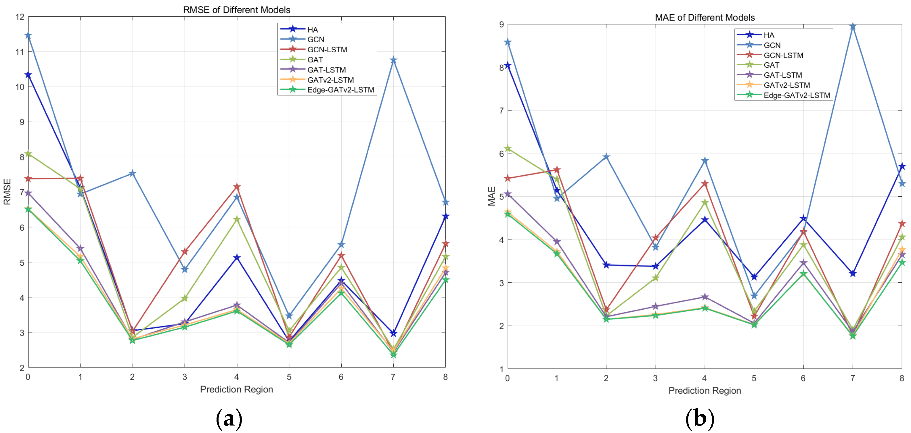
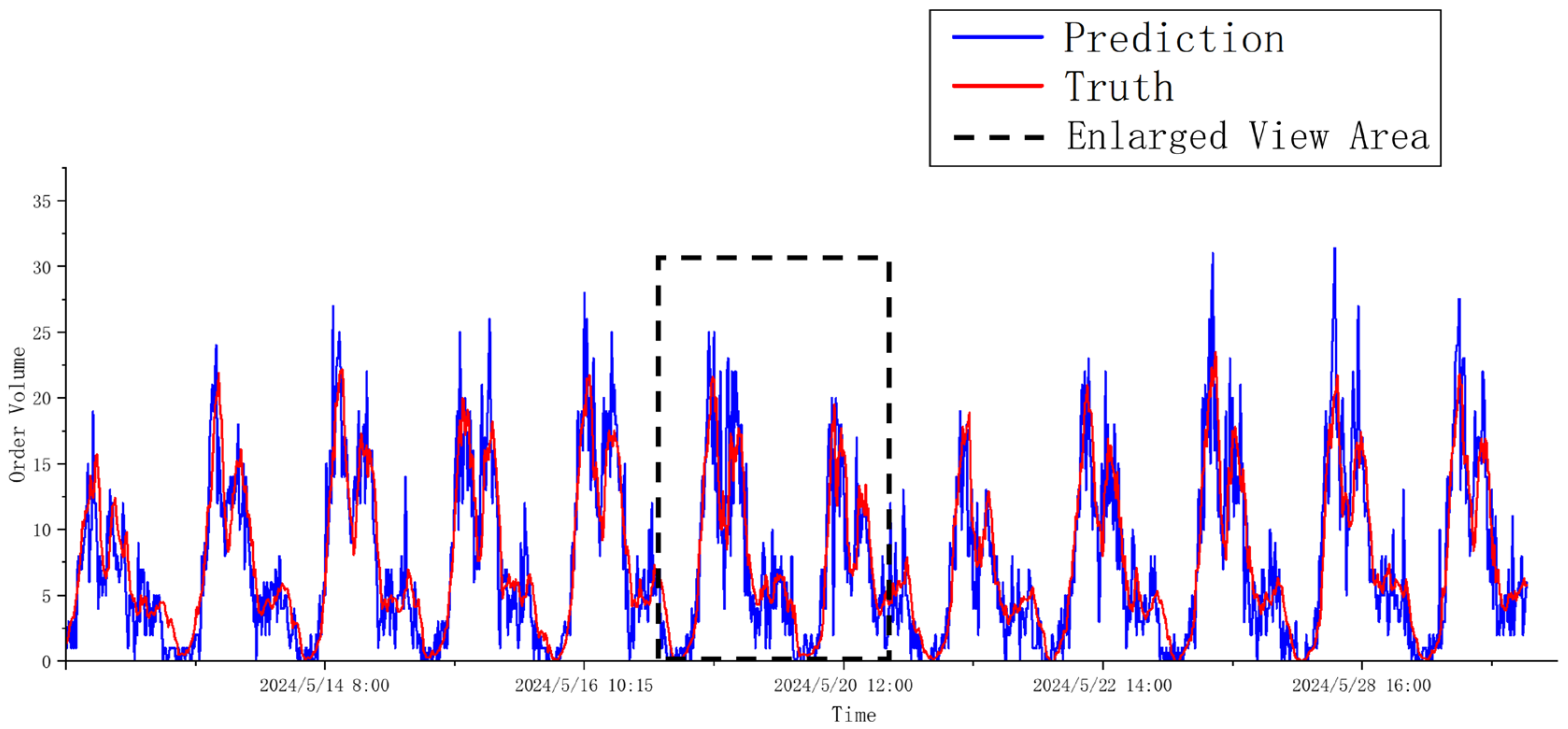
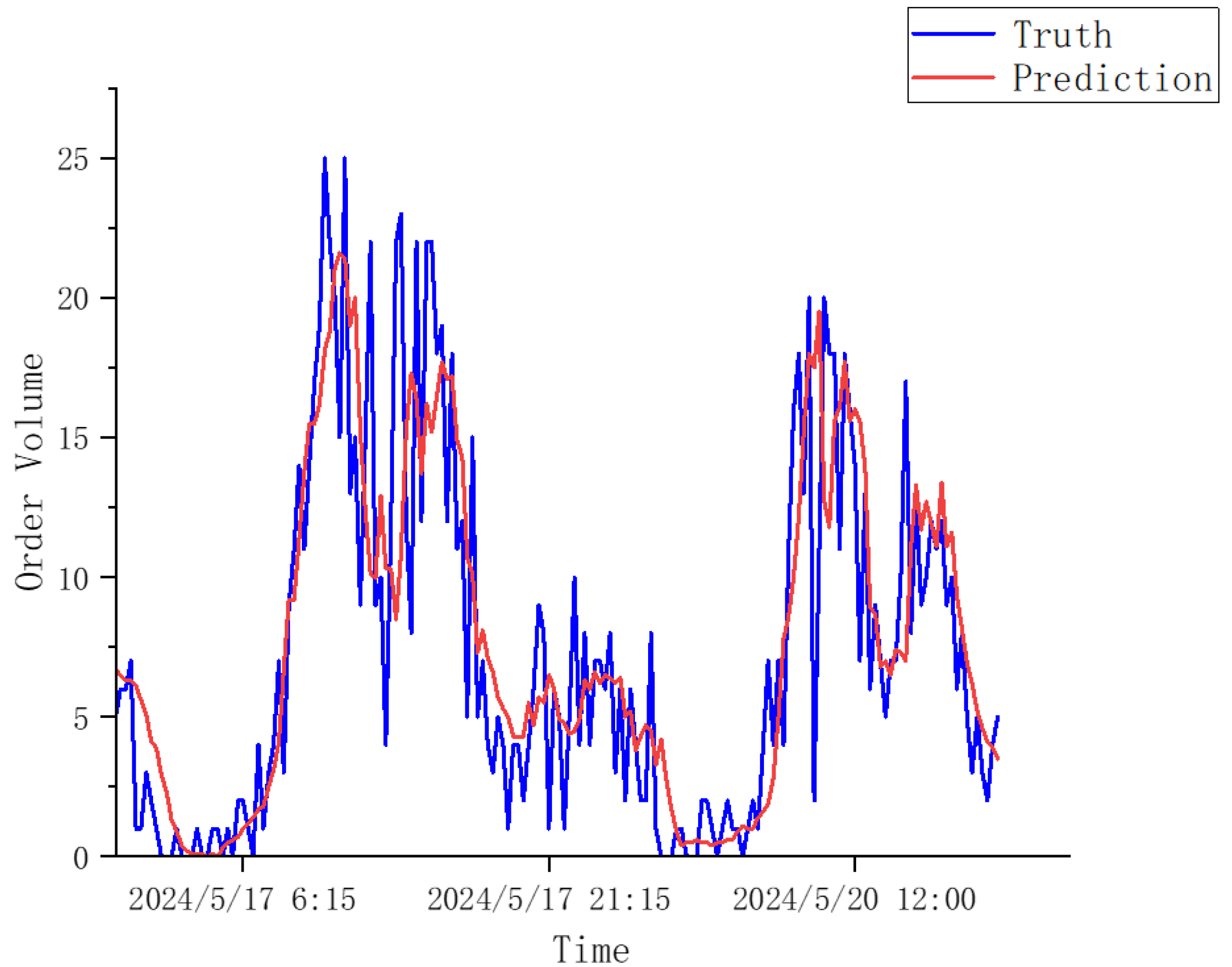
Experimental results based on real-world taxi data from Ningbo demonstrate that the Edge-GATv2-LSTM model outperforms four representative baselines—GCN, GCN-LSTM, GAT, and GAT-LSTM—achieving the lowest RMSE (3.85) and MAE (2.86). The model shows strong performance across different regions and peak periods, confirming the effectiveness of incorporating edge semantics into attention-based graph modeling.

The proposed model can provide useful support for several practical applications in urban transportation. For example, it can help taxi drivers identify where future pick-up demand is likely to be high so that they can plan routes more efficiently when vehicles are empty. The prediction results can also help platforms arrange vehicle dispatch in advance, balance supply and demand between regions, and improve service during rush hours. For traffic management departments, the model can support the monitoring of regional travel patterns and help design better traffic control strategies.

Future research can be carried out in the following directions. First, incorporating attention mechanisms into the LSTM component may further enhance the model’s ability to capture long-term fluctuations in taxi pick-up demand. Second, different combinations of graph neural network layers and temporal modeling units may have varying effects on performance; future work could explore more expressive architectures to further improve the prediction accuracy and generalization capability. Third, since this study is based solely on data from Ningbo, future studies could apply the proposed model to cities with different urban structures and mobility patterns to evaluate its transferability and robustness. Finally, external factors such as weather conditions, public holidays, and special events were not included in this study due to limited data availability. However, the proposed model can be adapted to incorporate such inputs in future work when relevant data become available.