Abstract
Route planning under uncertain traffic conditions requires accounting for not only expected travel times but also the risk of late arrivals. This study proposes a mean-upper partial moment (MUPM) framework for pathfinding that explicitly considers travel time unreliability. The framework incorporates a benchmark travel time to measure the upper partial moment (UPM), capturing both the probability and severity of delays. By adjusting a risk parameter (), the model reflects different traveler risk preferences and unifies several existing reliability measures, including on-time arrival probability, late arrival penalty, and semi-variance. A bi-objective model is formulated to simultaneously minimize mean travel time and UPM. Theoretical analysis shows that the MUPM framework is consistent with the expected utility theory (EUT) and stochastic dominance theory (SDT), providing a behavioral foundation for the model. To efficiently solve the model, an SDT-based label-correcting algorithm is adapted, with a pre-screening step to reduce unnecessary pairwise path comparisons. Numerical experiments using GPS probe vehicle data from Louisville, Kentucky, USA, demonstrate that varying values lead to different non-dominated paths. Lower values emphasize frequent small delays but may overlook excessive delays, while higher values effectively capture the tail risk, aligning with the behavior of risk-averse travelers. The MUPM framework provides a flexible, behaviorally grounded, and computationally scalable approach to pathfinding under uncertainty. It holds strong potential for applications in traveler information systems, transportation planning, and network resilience analysis.
1. Introduction
Travel times, especially in urban areas, vary widely due to fluctuating travel demand and roadway capacity at different times of the day and from day to day [1]. The variation often leads to unexpected late arrivals for work, appointments, deliveries, and so forth. To reduce the risk of being late, one must consider not just the average travel time, but also its variability in the route choice process [2,3]. Travelers respond to travel time variability differently, depending on their risk-taking preferences and trip importance. Travelers’ risk preferences can also be influenced by psychological traits, which affect how they perceive uncertainty and make routing decisions under time pressure [4]. For instance, de Palma and Picard [5] showed that 33.9% of their respondents were risk-seeking, 6.6% were risk-neutral, and 60.5% were risk-averse. Fujii and Kitamura [6] found that younger commuters usually budget more time for their trips as they often associate more significant consequences with late arrivals. Conversely, commuters tend to budget less time when the requirement on arrival time is less restrictive, for example, with a flexible work schedule in place. Therefore, it is critical for pathfinding models to not only incorporate travel time variability but also account for individual risk-taking behaviors and trip characteristics.
In recent decades, researchers have extended average travel time-based deterministic models by integrating various approaches to account for uncertainty in travel time [7]. Among them, the most common are the expected utility theory (EUT), stochastic dominance theory (SDT), and mean-risk approach.
The EUT assumes that travelers are rational and always choose routes that maximize their expected utilities [8]. These utilities are determined by specific utility functions, such as linear, exponential, or quadratic curves [8,9,10], which reflect different risk-taking attitudes. A major challenge associated with the EUT lies in selecting representative functions that characterize travelers’ actual route choice behaviors.
The SDT is known to be equivalent to unanimous choices made by the expected utility maximizers [11]. It establishes a partial order over a set of uncertain prospects without relying on predefined utility functions [12,13]. However, it can be computationally burdensome because it ranks prospects using pair-wise comparisons. Additionally, because SDT cannot establish a complete order, it often identifies a large number of admissible paths, especially in congested urban networks.
The mean-risk approach considers two simpler statistical measures: the average travel time and a risk measure that reflects travel time variability under undesirable conditions, typically on the right-hand side of a travel time distribution [2]. While these risk metrics share a general focus, following the framework by Chen and Zhou [14], they can be categorized into reliability- and unreliability-based measures.
From the reliability aspect, the travel time budget (TTB) approach defines a buffer time in addition to the mean to ensure a certain confidence level for on-time arrival [15,16,17]. The buffer is often computed as a multiplier of the standard deviation that reflects the relative importance of the reliability to the mean. The TTB approach assumes a normal distribution to maintain a one-to-one relationship between confidence level and the multiplier. However, Wu and Nie [11] argue that the confidence level is more in line with the trip’s importance rather than the traveler’s intrinsic risk-taking attitude.
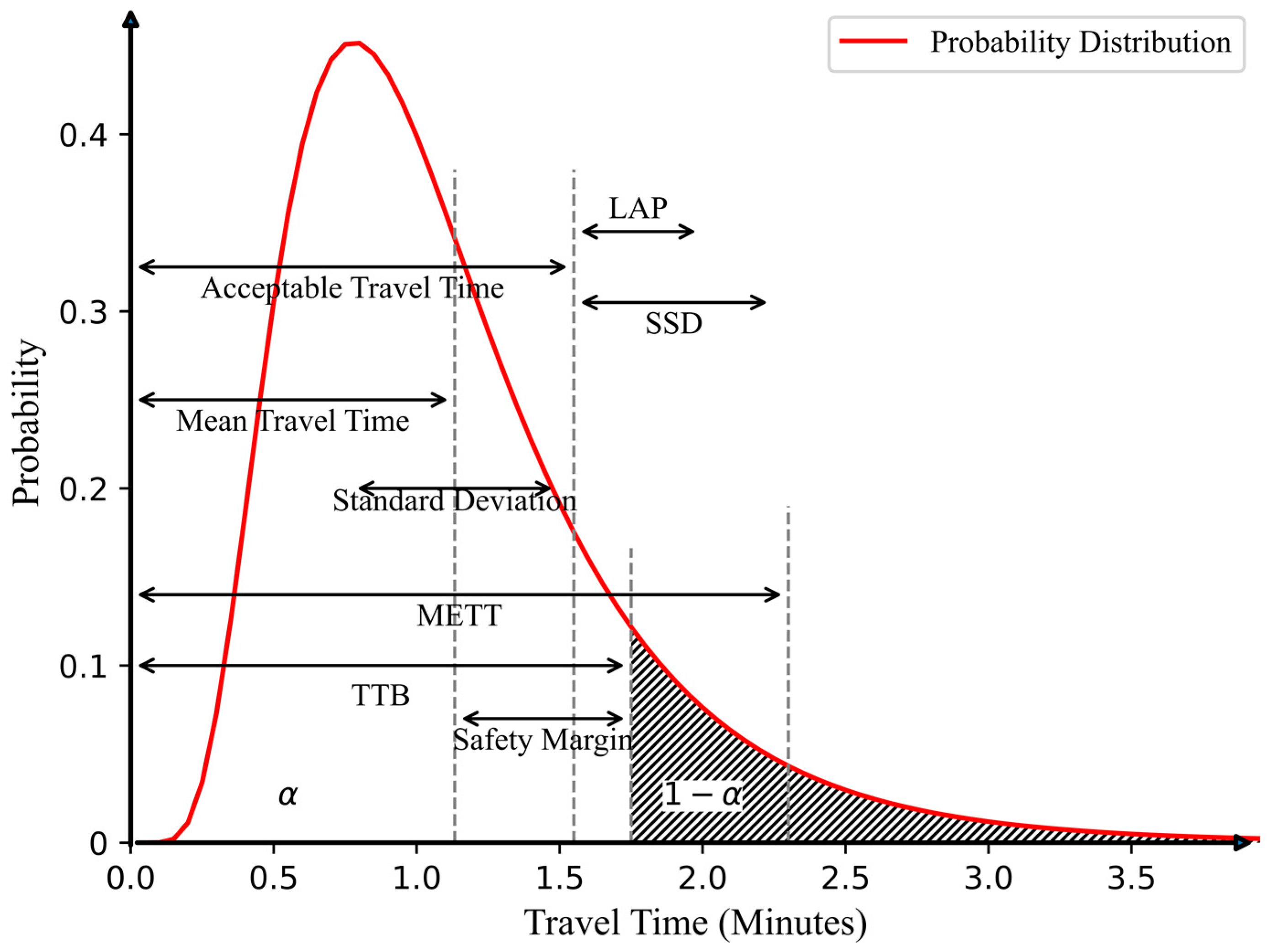
A similar approach is the on-time arrival probability (OTAP) model, which maximizes the probability of arriving on time given a fixed travel time constraint [18,19,20,21,22]. Both TTB and OTAP focus on the “reliable” portion up to of the travel time distribution, but ignore the tail risks associated with longer travel times that fall beyond , as illustrated in Figure 1. This shortcoming becomes more apparent when travel time distribution is skewed with a longer right tail.
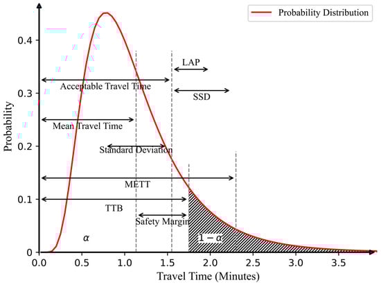
Figure 1.
Illustration of various travel time reliability measures relative to a given travel time distribution curve.
To address this limitation, alternative measures have been proposed. The semi-standard deviation (SSD) focuses on the right side of the distribution beyond a benchmark travel time [23,24]. The benchmark can be the mean or other values deemed acceptable by the traveler [25]. The mean excess travel time (METT) measures the conditional expectation of travel times exceeding the TTB [14]. In addition, the late arrival penalty (LAP) quantifies the penalty incurred from late arrivals as a result of travel times exceeding the acceptable threshold [26]. However, the LAP model lacks an optimization method and may not be able to fully capture the unreliability [27]. Figure 1 provides visual representations of these measures.
Despite progress in developing risk measures, their theoretical relationships and behavioral interpretations remain underexplored. This is an important issue because understanding how these measures align with different risk attitudes can guide a more effective model selection. For instance, Wu and Nie [11] assessed the rationality of several measures from the perspective of the SDT and showed that the TTB and mean-variance approaches comply with the SDT only under a quadratic utility function (QUF). Meanwhile, OTAP and METT satisfy the first-order dominance rule, which in itself does not differentiate risk attitudes. Tan et al. [28] investigated the association of TTB, OTAP, METT, and QUF with the mean-standard deviation model. They found that TTB and QUF correspond to risk-averse plunging and diversifying behaviors, while the link between OTAP or METT and such behaviors depends on travel time distribution. Wang et al. [29] showed that the mean-standard deviation model encompasses TTB and LAP when travel times follow a normal distribution. However, the applicability of the mean-standard deviation characterization for rational travelers is limited to quadratic utility function or normally distributed travel times [30].
In this paper, we propose a generic framework based on the mean and upper partial moment (UPM). The UPM focuses on the right side of the travel time distribution to reflect the traveler’s concern over long travel times [7]. It relaxes the assumption about the underlying distribution, making it more realistic than other risk measures, including the widely used standard deviation. It also accommodates different risk-taking behaviors and trip importance through parameter adjustments. The framework encompasses several existing risk measures, including OTAP, LAP, and SSD, which enables us to evaluate their attributes and relationships. Importantly, it is consistent with EUT and SDT, offering both a behavioral basis and computational efficiency by adapting a dynamic programming algorithm developed for SDT. The use of the UPM draws inspiration from the lower partial moment in portfolio theory, which aims to maximize returns while controlling downside risk [31,32,33]. Here, we instead aim to minimize the average travel time and the risk of arriving later than an acceptable benchmark.
The rest of the paper is organized as follows: Section 2 introduces the proposed mean-UPM (MUPM) framework and formulates a bi-objective pathfinding model, which accounts for correlated link travel times using a sampling-based approach. Section 3 explores the framework’s theoretical consistency with classical theories, including EUT and SDT, which enables the efficient solution algorithm described in Section 4. Section 5 presents numerical experiments using a real-world network and travel time data. Section 6 summarizes the findings to conclude the paper.
2. The Mean-Upper Partial Moment Framework
Table 1 defines the key symbols that are used in this paper for the mathematical modeling and proofs.

Table 1.
Key symbols used in the subsequent mathematical formulas and proofs.
2.1. The Upper Partial Moment as the Risk Measure
Consider a strongly connected network , where is the set of nodes, is the set of links, and is the set of travel time distributions associated with the links. Let and represent the origin and destination node, respectively. Let be the random travel time on path , where denotes the set of paths from to . The path travel time follows probability distribution with a cumulative distribution function . Assume that the traveler knows this distribution at a fixed departure time and selects a route based on a travel time benchmark . The late arrival occurs when . Now let be the mean and be the UPM of on with respect to the benchmark . The UPM is defined as
The benchmark reflects the traveler’s acceptable arrival time, which follows the same idea in Watling [26]. Trips with a flexible schedule can tolerate longer travel times and thus justify a larger . Conversely, trips with stricter arrival requirements, such as job interviews or scheduled deliveries, warrant a smaller to reduce the risk of being late.
The risk parameter controls the sensitivity of the UPM to late arrivals. When , short delays have a disproportionate effect on the UPM compared with long ones. When approaches 0, all delays, regardless of magnitude, have an equal impact. When , the UPM becomes , which is the LAP in Watling [26]. When , longer delays exert a greater impact on the UPM than short ones. The impact increases more significantly as increases. At , the UPM becomes the semi-variance, which is sensitive to excessive delays [25].
It should also be noted that when , the UPM reduces to a probability measure:
where is the on-time arrival probability (OTAP). Therefore, minimizing the UPM at is equivalent to maximizing OTAP.
To estimate a traveler’s risk preference , one can apply a simple process from Fishburn [32]. Consider two routes: one with a deterministic travel time and the other with a probabilistic travel time of either (with probability ) or (with probability ). The respective UPMs are and . If the traveler is indifferent to either route at , meaning , then we obtain . For example, yields , or yields , or yields . With detailed GPS trajectory data [34], empirical methods (e.g., Zeng, et al. [35]) can be used to determine more accurately.
2.2. The Bi-Objective Pathfinding Model
Travelers may have multiple requirements on the on-time arrivals under both normal and unpredictable congested conditions. Most existing studies combine the mean and risk measure into a single objective using a fixed weight. However, this approach may not fully represent the traveler’s preference or cover other rational alternatives [29]. To address this, we formulate a bi-objective mean-UPM (MUPM) model that minimizes both the expected travel time and UPM. This formulation allows for a trade-off analysis among identified alternatives to select the most preferred path.
Similar to [29], we define the following dominance relationships using both objectives.
Definition 1.
A path dominates a path by the MUPM rule or , if and with at least one strict inequality.
Definition 2.
A path is an MUPM non-dominated path if and only if no such path exists such that .
To compute a path’s UPM, we must account for potential correlations among link travel times, as congestion and delays often propagate across connected links in real-world networks. However, due to the nonlinear form of Equation (1), no closed-form equation exists to aggregate link-level UPMs into a path-level measure [24]. To address this, we apply a sampling-based approach [36]. The approach implicitly captures the correlation structure underlying link-level travel time observations without knowing the exact correlation matrix. Suppose that there are discrete travel time realizations for each link, and let denote the travel time on link at time interval . Let be the binary variable, where if link is a member link of path and otherwise. For each time interval , the path travel time is . The distribution of path travel times can then be obtained from all time intervals. Because the observed path-level samples reflect actual network dynamics, the dependence among link travel times, such as spillbacks or coordinated signals, is embedded in the joint outcomes. This approach assumes that traffic conditions on individual links stay the same as the traveler traverses the path. This assumption can be relaxed with a dynamic approach considering the actual travel time when the traveler arrives at each link; however, this is outside the scope of this paper.
Accordingly, we can determine the mean and UPM of the path travel time as follows:
Therefore, the bi-objective MUPM model can be reformulated as follows:
Equations (5) and (6) are to minimize the average travel time and UPM, respectively. Equation (7) ensures that all the links on the path are feasible. Equation (8) defines a binary link-path incidence variable.
3. Consistency Between MUPM and Classic Theories
This section investigates the theoretical connections between the MUPM framework and the EUT and SDT. Establishing these links reinforces the behavioral validity of the MUPM framework and facilitates the development of a solution algorithm.
3.1. Expected Utility Theory
To reflect the traveler’s negative perception of long travel times, we adopt the disutility concept, commonly used in transportation studies. Assume that the traveler’s disutility function with respect to experienced travel times is , which increases as the travel time increases. Accordingly, the traveler is considered risk-seeking if is concave, risk-neutral if is linear, or risk-averse if is convex. Readers are directed to Yin and Ieda [8] for a detailed discussion on risk-taking behaviors. Then, based on the EUT, the traveler prefers path over if
The MUPM framework assumes that the traveler’s disutility can be adequately represented by the mean and UPM. Assume that is such disutility function that increases with both the mean and the UPM . Then, the preference is given to path over if
Therefore, to show the consistency between the EUT and MUPM, we must prove that there exists a disutility function such that Equation (10) holds if Equation (9) holds.
Proposition 1.
The MUPM framework is consistent with the EU theory in the sense that there exists a such that if .
Proof.
Assume that the disutility function is as follows, with being a positive constant:
Then, the expected disutility becomes
where is the only solution to , since
Given , we can have . □
Based on the proposition above, the MUPM framework is equivalent to the EUT with the disutility function given by Equation (11). The constant is often referred to as reliability ratio, which represents the relative importance of the reliability compared with the mean.
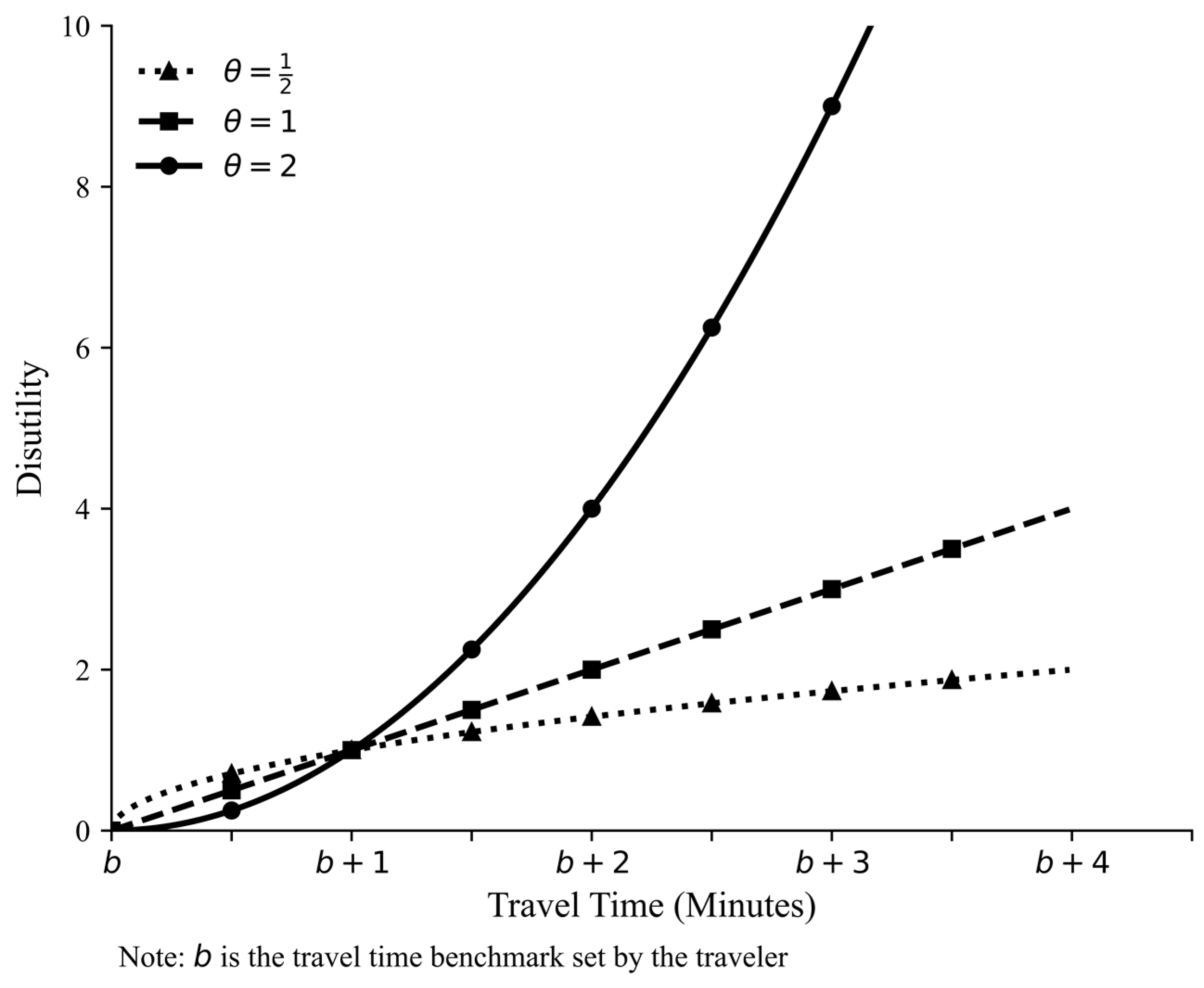
It is clear that the disutility function is linear below the benchmark , reflecting a risk-neutral attitude towards on-time arrivals. For travel times above the benchmark, i.e., the unreliability portion of the distribution, the shape of the disutility function depends on . When , the disutility function is linear, meaning that the traveler is risk-neutral towards delays. In other words, the traveler is indifferent to alternative paths when their average delays are the same. When , the disutility curve is concave, depicting the risk-seeking behavior. In this case, the traveler’s main concern is later arrival but with less regard to the amount of delay. As a result, the traveler is willing to choose the path with a small probability of encountering excessively long delays. Furthermore, when , the disutility curve is convex, and the traveler is risk-averse and highly sensitive to excessively long delays. Figure 2 illustrates the disutility curves of the deviations over the benchmark in terms of several specific values with set to 1.
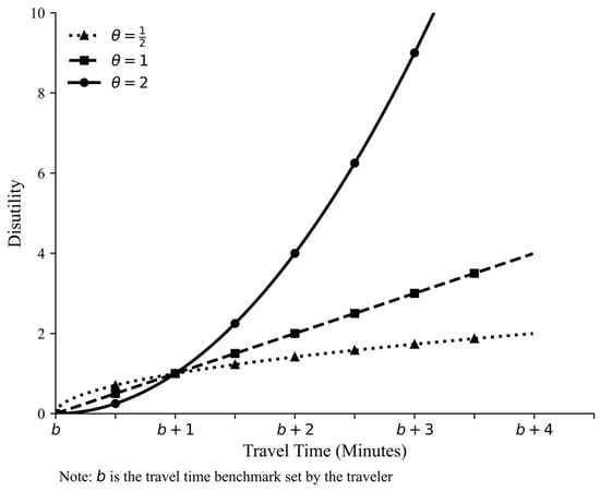
Figure 2.
Illustration of different disutility curves of the deviations over the benchmark (b) with respect to three specific values.
Because it is difficult to estimate a realistic value and a single-objective function may overlook rational alternatives, the bi-objective MUPM formulation is preferred as a more generic framework to model the pathfinding problem.
3.2. Stochastic Dominance Theory
To further validate the behavioral basis of the MUPM, we examine its relationship with the SDT. The definitions of the first three SDT rules in the context of the pathfinding process following Wu and Nie [11] are first provided.
Definition 3.
Path dominates path by the first-order stochastic dominant (FOSD) rule or , if , for all values of , with the strict inequality holds for at least one .
Definition 4.
Path dominates path by the second-order stochastic dominant (SOSD) rule or , if with , for all values of , with the strict inequality holds for at least one .
Definition 5.
Path dominates path by the third-order stochastic dominant (TOSD) rule or , if with , for all values of , with the strict inequality holds for at least one .
Here, we denote , , and as a non-dominated path set with respect to FOSD, SOSD, and TOSD rules, respectively. It has been shown that the non-dominated path set in terms of an FOSD rule contains that in terms of an SOSD rule, which contains that in terms of a TOSD rule, . Additionally, if , then with the strict inequality holds for an FOSD dominance condition [11,23]. Building on those findings, the following propositions establish the connection between the MUPM and the SDT.
Proposition 2.
The optimal solutions to the MUPM model with is a subset of the FOSD non-dominated paths.
Proof.
If , we can directly have
If , then by applying the integration by parts, we have:
Therefore, we can obtain
It is easy to know as . Recall that when , . Accordingly, we can know , i.e., .
In the meantime, it is known that if . □
Proposition 3.
The optimal solutions to the MUPM model with is a subset of the SOSD non-dominated paths, except when and .
Proof.
With , we know . By applying the integration by parts on in Equation (14), we can obtain
Recall that if , then . Therefore, Equation (16) gives . At the same time, if , then . □
Proposition 4.
The optimal solutions to the MUPM model with is a subset of the TOSD non-dominated paths, except when and .
Proof.
First of all, . Therefore, . Next, we apply the integration by parts once again on in Equation (16) and obtain
Based on the TOSD definition, if , . Accordingly, . Similarly, if , then . □
Accordingly, depending on the value of , the MUPM non-dominated path set is nested within the non-dominated sets defined by SDT rules, with very mild exceptions for SOSD and TOSD rules. The exception arises only when an MUPM non-dominated path is dominated by an SOSD or TOSD non-dominated path. As a result, we could omit this path when we choose the MUPM non-dominated paths from the SOSD or TOSD non-dominated path set. Nonetheless, such exception does not undermine the consistency of MUPM with the SDT, as at least one path with an identical mean and UPM would be retained. Thus, the MUPM framework aligns well with both the EUT and SDT, providing a valid behavioral basis for modeling a pathfinding problem under uncertainty.
4. Solution Algorithm
Due to the non-additive property of the UPM, classical algorithms, e.g., Dijkstra’s algorithm, are no longer applicable for the proposed framework. Researchers have developed several alternative approaches for pathfinding under non-additive risk measures, including mathematical programming, simulation-based methods, and evolutionary algorithms [19,25,37,38,39,40,41]. Among these, the SDT-based label-correcting (LC) approach has demonstrated computational efficiency in the large networks under both continuous and discrete travel time distributions [11,13,42]. Given the established consistency between the MUPM and the SDT, we adapt the SDT-based LC algorithm to find MUPM non-dominated paths.
One limitation of the SDT approach is the need for exhaustive pairwise comparisons between path distributions to determine the dominance relationship. In particular, even after we know that the first path does not dominate the second one, we still need to determine whether the second path dominates the first one. This is computationally burdensome when the number of paths under consideration is large. To reduce the number of unnecessary comparisons, we introduce the following proposition:
Proposition 5.
If , then , where and represent the minimum travel time on and , respectively.
Proof.
Suppose that there is a travel time observation such that ; then we can easily obtain . As a result, . First, this directly contradicts the FOSD rule. Second, integrating over the range generates a negative value, which also violates the SOSD and TOSD requirements. □
As a result, Proposition 5 along with the necessary condition of the mean under SDT rules can eliminate unnecessary comparisons by first examining the minimum and mean travel times on two paths. Suppose that there are three alternative paths. To obtain the non-dominated paths, the maximum number of pairwise comparisons is six. Now assume that the minimum travel time on those paths are known and follow the order of . Based on Proposition 5, we can eliminate half of these comparisons. For instance, it is clear that would not be preferred to ; otherwise, it is a violation of Proposition 5. In addition, if the mean travel times are obtained and follow the order of , this additional condition further reduces the number of comparisons to one, i.e., whether dominates . As a result, the efficiency of the solution procedure can be significantly improved. The SDT-based LC procedure with an additional screening step is in Algorithm 1 as follows:
| Algorithm 1. Modified SDT-LC Algorithm |
| Step 1: Initialization. Let be the path from to itself and be the discrete travel time, which are zero. Initialize the scan list . Step 2: Select the first path from , and denote it as ; then delete it from . Step 3: For any predecessor node of and that is not contained in the current , create a new path , and update the path travel time , and then obtain the set of unique travel time realizations of path . Step 4: Quick dominance screening. Compare and of path with those of path , where is the existing non-dominated path set according to the particular dominance rule of interest. If and , check if path dominates path ; else, if and , check if path dominates path . Otherwise, keep and update and ; then go to Step 2. Step 5: Distributional dominance evaluation. Suppose that we now need to check whether dominates . Depending on the particular dominance rule under evaluation: (a) FOSD dominance: if for all , and for at least one ; (b): SOSD dominance: if for all , and for at least one ; (c): TOSD dominance: if for all , and for at least one . Drop and update and . Otherwise, drop and go to Step 6. Step 6: If is empty, go to Step 7; otherwise, go to Step 2. Step 7: Identify and output the MUPM non-dominated path set . |
5. Numerical Experiments
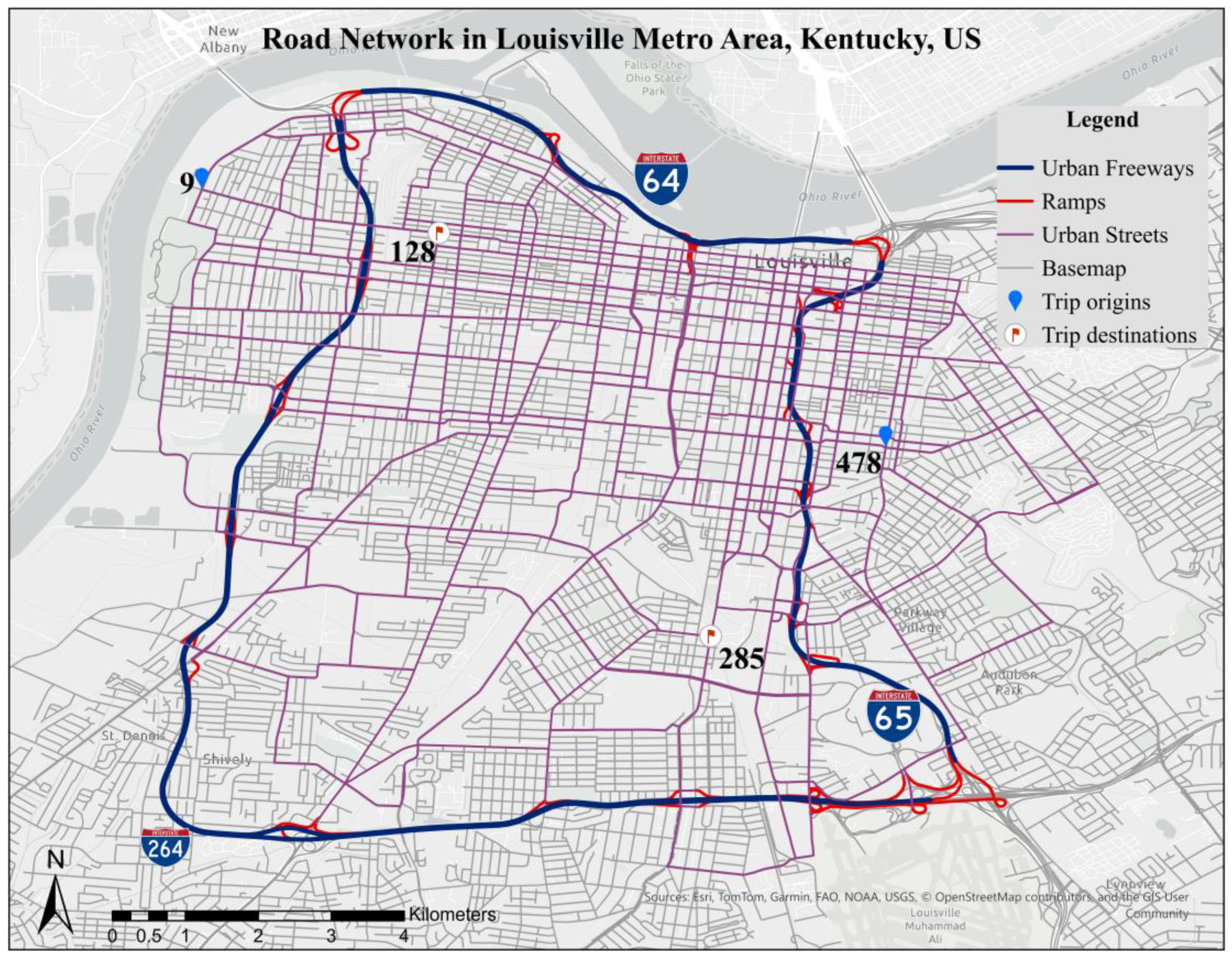
In this section, a real-world network and measured travel time data are used to evaluate the MUPM framework. The network is from the Louisville Metro area in Kentucky, USA, consisting of 528 nodes and 1269 links, as shown in Figure 3. The network-wide travel time data are collected from GPS probe vehicle data with 15 min increments by time of day and day of week for each month. This analysis focuses on the weekday afternoon peak period from 3 pm to 6 pm. Each link has 720 individual travel time observations (12 months 5 weekdays 3 h 4 intervals). Based on the skewness and kurtosis statistics, over 99% of links exhibit positively skewed and leptokurtic distributions with long right tails. This observation justifies the use of asymmetrical risk measures such as the UPM to emphasize the right tail of distributions.
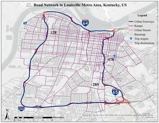
Figure 3.
Louisville Metro area road network and locations of selected trip origins and destinations.
We choose two OD pairs to perform more detailed analyses. One is from node 128 to node 478 within the downtown area, and the other is from node 285 to node 9, which represents a cross-city trip. The locations of those OD pairs are illustrated in Figure 3. To evaluate different risk preferences, four MUPM models with different values are tested: . The case is included for the purpose of comparison. The SDT-LC algorithm in terms of the FOSD rule is applied to determine the non-dominated paths for all four MUPM models for each OD pair. The benchmark travel time is set as the minimum average travel time for each OD pair, i.e., 19.604 min for OD 128–478 and 22.18 min for OD 285–9.
Table 2 presents the identified non-dominated paths, their mean travel times, UPM values, and 90th, 95th, and 99th percentile travel times (PTTs), which characterize the tail of each path’s distribution. It can be seen that there is no single optimal path in both the average travel time and UPM, underscoring the need for considering travel time variability in the pathfinding model.
Table 2.
Non-dominated paths for the two OD pairs.
With , the UPM reduces to the OTAP measure. The MUPM non-dominated paths are determined based on the mean and probability values at the benchmark. As discussed in Section 1, OTAP ignores the portion of the distribution beyond the benchmark, even though it may be a “fat tail” that is associated with frequent late arrivals. For OD 128–478, Paths 1, 2, 3, 5, and 6 show a smaller UPM (or higher OTAP) and are considered non-dominated. However, Paths 5 and 6 experience noticeably longer 95th and 99th percentile travel times, suggesting frequent excessive delays despite good OTAP performance. In contrast, Path 4, although dominated in OTAP, has the shortest 95th and 99th percentile travel times, indicating lower exposure to extensive delays. Similarly, for OD 285–9, Paths 1 and 2 clearly dominate Path 3 and 4 in OTAP. However, the long tail of Path 2′s travel time distribution indicates that it experiences more frequent excessive delays compared with other paths.
When , the MUPM reflects the risk-seeking behavior of the traveler, who worries more about being late but is less concerned about how late. In this case, the effects of small delays are heightened, whereas the effects of long delays are reduced. Therefore, the UPM is more sensitive to the portion of the distribution with small delays but less responsive to the tail of the distribution composed of long delays. For this reason, Paths 2 and 3 are preferred to Path 4 for OD 128–478, even though they are more likely to encounter very long delays, as indicated by 95th and 99th percentile travel times. Similarly, despite the long tail, Path 2 is preferred to Paths 3 and 4 for OD 285–9.
When , the UPM becomes the LAP measure, reflecting the risk-neutral attitude towards the delays beyond the benchmark. The measure focuses on the average delay and is linearly proportional to the distribution of small and long delays. As a result, Path 4 joins the non-dominated path set for OD 128–478, because it has the smallest average delay, despite its worse OTAP. Likewise, Path 3 turns out to be the optimal path in terms of the expected delay for OD 285–9.
As increases to 2, the UPM becomes the semi-variance and reflects the risk-averse attitude of the traveler, who is more concerned about the excessively long delays. In this case, the UPM penalizes these long delays disproportionately and thus is more sensitive to the tail end of the travel time distribution. For OD128–478, Path 2, despite being the non-dominated path under the risk-neutral scenario, is now dominated by Path 1 due to its longer tail, as reflected by the 95th and 99th percentile travel times. For OD 285–9, Path 4 becomes the optimal path in terms of the UPM due to its shorter tail and reduced risk of excessive delays compared with other paths.
6. Conclusions
This study addresses the critical issue of incorporating travel time uncertainty into the pathfinding problem from the perspective of traveler decision making. Motivated by the fact that the traveler’s main concern is the risk of being late, we propose an effective mean-upper partial moment (MUPM) framework. The UPM focuses on the right-hand side of the travel time distribution and, therefore, intuitively aligns with the traveler’s late arrival concern. The framework is generic in the sense that it is able to reflect the importance of a trip and the consequence of late arrival without assuming a certain distribution function.
One of the core contributions of this study is the demonstration that the MUPM framework unifies several existing reliability measures, including on-time arrival probability, late arrival penalty, and semi-variance, within a single, generalized structure. By varying the parameter, the MUPM model effectively distinguishes between risk-seeking (, risk-neutral (), and risk-averse ( travel behavior. This feature not only offers a behavioral interpretation of risk preferences but also provides a means to systematically evaluate the implications of different reliability measures under a common framework.
This study also demonstrates theoretical consistency between the MUPM model and the classical expected utility theory (EUT) and stochastic dominance theory (SDT). The EUT consistency provides a foundation for interpreting different traveler risk preferences based on the curvature of the disutility function. Meanwhile, the SDT consistency enables the adaption of a label-correcting algorithm to identify non-dominated paths under the MUPM, leveraging SDT dominance rules. A screening condition based on minimum and mean travel times is introduced to reduce computational complexity, improving the efficiency and scalability of the solution approach in large-scale transportation applications.
To evaluate its practical applicability, the proposed framework is applied to a real-world network in the Louisville Metro area using GPS probe vehicle data. The numerical experiments confirm that different θ values yield different sets of non-dominated paths, reflecting varying levels of sensitivity to delays beyond the benchmark. Notably, using (OTAP) may select paths that are prone to excessive delays, underscoring its limitation in accounting for the unreliability portion of the travel time distribution. Conversely, setting captures the tail risk more effectively, especially the delays beyond the 95th percentile travel time, better aligning with the behavior of risk-averse travelers.
The MUPM framework offers a clear practical value for traveler information and transportation planning systems. It provides a more realistic and customizable approach to route guidance by incorporating individual risk preferences, such as minimizing small but frequent delays for risk-seeking travelers or avoiding infrequent but excessive delays for risk-averse ones. The model also provides transportation planners a flexible tool to evaluate and compare alternative routes or network improvements under uncertainty, particularly in urban areas with high variability in travel times. The MUPM framework can also help inform resilience planning under uncertain traffic conditions.
Future studies can explore how an actual risk-taking behavior varies by traveler type or trip purpose by analyzing GPS traces or state preference data. This would allow for an empirical calibration of values and benchmark travel times across different groups. Moreover, expanding the numerical study to cover more time periods and geographical areas can demonstrate the generalizability of the framework. In addition, comparing the MUPM framework with alternative unreliability models, such as the Mean-Excess Travel Time model, would provide further insights into the relative strengths and limitations of different approaches to modeling travel time unreliability.
Author Contributions
Conceptualization, X.Z.; data curation, X.Z.; formal analysis, X.Z. and M.C.; funding acquisition, M.C.; methodology, X.Z.; supervision, M.C.; validation, X.Z. and M.C.; writing—original draft, X.Z.; writing—review and editing, X.Z. and M.C. All authors have read and agreed to the published version of the manuscript.
Funding
This research received no specific grant from any funding agency in the public, commercial, or not-for-profit sectors.
Data Availability Statement
The road network data are publicly available at https://transportation.ky.gov/Planning/Pages/Centerlines.aspx, access on 20 June 2025. The travel time data provided by the data vendor cannot be shared subject to the licensing restriction.
Conflicts of Interest
The authors declare no potential conflicts of interest with respect to the research, authorship, and/or publication of this article.
Abbreviations
The following abbreviations are used in this manuscript:
| EUT | expected utility theory |
| SDT | stochastic dominance theory |
| TTB | travel time budget |
| OTAP | on-time arrival probability |
| SSD | semi-standard deviation |
| METT | mean excess travel time |
| LAP | late arrival penalty |
| QUF | quadratic utility function |
| UPM | upper partial moment |
| MUPM | mean-upper partial moment |
| PTT | percentile travel time |
| LC | label correcting |
References
- Paricio-Garcia, A.; Lopez-Carmona, M.A. Impact of Static Urban Traffic Flow-Based Traffic Weighted Multi-Maps Routing Strategies on Pollutant Emissions. Systems 2024, 12, 89. [Google Scholar] [CrossRef]
- Carrion, C.; Levinson, D. Value of Travel Time Reliability: A Review of Current Evidence. Transp. Res. Part A Policy Pract. 2012, 46, 720–741. [Google Scholar] [CrossRef]
- Ge, Y.; Sun, Y.; Zhang, C. Modeling a Multimodal Routing Problem with Flexible Time Window in a Multi-Uncertainty Environment. Systems 2024, 12, 212. [Google Scholar] [CrossRef]
- Li, Y.; Zhang, Y.; Liu, S. The myths of successful expatriation: Does higher emotional intelligence lead to better cultural intelligence? Int. Bus. Rev. 2025; in press. [Google Scholar] [CrossRef]
- de Palma, A.; Picard, N. Route choice decision under travel time uncertainty. Transp. Res. Part A Policy Pract. 2005, 39, 295–324. [Google Scholar] [CrossRef]
- Fujii, S.; Kitamura, R. Drivers’ Mental Representation of Travel Time and Departure Time Choice in Uncertain Traffic Network Conditions. Netw. Spat. Econ. 2004, 4, 243–256. [Google Scholar] [CrossRef]
- Zang, Z.; Batley, R.; Xu, X.; Wang, D.Z.W. On the value of distribution tail in the valuation of travel time variability. Transp. Res. Part E Logist. Transp. Rev. 2024, 190, 103695. [Google Scholar] [CrossRef]
- Yin, Y.; Ieda, H. Assessing Performance Reliability of Road Networks Under Nonrecurrent Congestion. Transp. Res. Rec. J. Transp. Res. Board 2001, 1771, 148–155. [Google Scholar] [CrossRef]
- Mirchandani, P.; Soroush, H. Generalized Traffic Equilibrium with Probabilistic Travel Times and Perceptions. Transp. Sci. 1987, 21, 133. [Google Scholar] [CrossRef]
- Monroe, T.; Beruvides, M.; Tercero-Gómez, V. Quantifying Risk Perception: The Entropy Decision Risk Model Utility (EDRM-U). Systems 2020, 8, 51. [Google Scholar] [CrossRef]
- Wu, X.; Nie, Y. Modeling Heterogeneous Risk-Taking Behavior in Route Choice: A Stochastic Dominance Approach. Transp. Res. Part A Policy Pract. 2011, 45, 896–915. [Google Scholar] [CrossRef]
- Miller-Hooks, E.; Mahmassani, H. Path comparisons for a priori and time-adaptive decisions in stochastic, time-varying networks. Eur. J. Oper. Res. 2003, 146, 67–82. [Google Scholar] [CrossRef]
- Xiao, L.; Lo, H.K. Adaptive vehicle routing for risk-averse travelers. Transp. Res. Part C Emerg. Technol. 2013, 36, 460–479. [Google Scholar] [CrossRef]
- Chen, A.; Zhou, Z. The α-reliable mean-excess traffic equilibrium model with stochastic travel times. Transp. Res. Part B Methodol. 2010, 44, 493–513. [Google Scholar] [CrossRef]
- Lo, H.K.; Lou, X.W.; Siu, B.W.Y. Degradable Transport Network: Travel Time Budget of Travelers with Heterogeneous Risk Aversion. Transp. Res. Part B Methodol. 2006, 40, 792–806. [Google Scholar] [CrossRef]
- Ji, Z.; Kim, Y.S.; Chen, A. Multi-objective α-reliable path finding in stochastic networks with correlated link costs: A simulation-based multi-objective genetic algorithm approach (SMOGA). Expert Syst. Appl. 2011, 38, 1515–1528. [Google Scholar] [CrossRef]
- Chen, B.Y.; Lam, W.H.K.; Sumalee, A.; Li, Z.-l. Reliable shortest path finding in stochastic networks with spatial correlated link travel times. Int. J. Geogr. Inf. Sci. 2012, 26, 365–386. [Google Scholar] [CrossRef]
- Fan, Y.; Nie, Y. Optimal routing for maximizing the travel time reliability. Netw. Spat. Econ. 2006, 6, 333–344. [Google Scholar] [CrossRef]
- Nie, Y.; Wu, X. Shortest Path Problem Considering On-Time Arrival Probability. Transp. Res. Part B Methodol. 2009, 43, 597–613. [Google Scholar] [CrossRef]
- Zeng, W.; Miwa, T.; Wakita, Y.; Morikawa, T. Application of Lagrangian relaxation approach to α-reliable path finding in stochastic networks with correlated link travel times. Transp. Res. Part C Emerg. Technol. 2015, 56, 309–334. [Google Scholar] [CrossRef]
- Yang, L.; Zhou, X. Optimizing on-time arrival probability and percentile travel time for elementary path finding in time-dependent transportation networks: Linear mixed integer programming reformulations. Transp. Res. Part B Methodol. 2017, 96, 68–91. [Google Scholar] [CrossRef]
- Jin, Z.; Mao, H.; Chen, D.; Li, H.; Tu, H.; Yang, Y.; Attard, M. Multi-objective optimization model of autonomous minibus considering passenger arrival reliability and travel risk. Commun. Transp. Res. 2024, 4, 100152. [Google Scholar] [CrossRef]
- Wu, X. Study on mean-standard deviation shortest path problem in stochastic and time-dependent networks: A stochastic dominance based approach. Transp. Res. Part B Methodol. 2015, 80, 275–290. [Google Scholar] [CrossRef]
- Zhang, X.; Chen, M. Genetic Algorithm–Based Routing Problem Considering the Travel Reliability Under Asymmetrical Travel Time Distributions. Transp. Res. Rec. J. Transp. Res. Board 2016, 2567, 114–121. [Google Scholar] [CrossRef]
- Zhang, X.; Chen, M. Bi-objective routing problem with asymmetrical travel time distributions. J. Intell. Transp. Syst. 2018, 22, 87–98. [Google Scholar] [CrossRef]
- Watling, D. User equilibrium traffic network assignment with stochastic travel times and late arrival penalty. Eur. J. Oper. Res. 2006, 175, 1539–1556. [Google Scholar] [CrossRef]
- Li, H.; Tu, H.; Hensher, D.A. Integrating the mean–variance and scheduling approaches to allow for schedule delay and trip time variability under uncertainty. Transp. Res. Part A Policy Pract. 2016, 89, 151–163. [Google Scholar] [CrossRef]
- Tan, Z.; Yang, H.; Guo, R. Pareto efficiency of reliability-based traffic equilibria and risk-taking behavior of travelers. Transp. Res. Part B Methodol. 2014, 66, 16–31. [Google Scholar] [CrossRef]
- Wang, J.Y.T.; Ehrgott, M.; Chen, A. A bi-objective user equilibrium model of travel time reliability in a road network. Transp. Res. Part B Methodol. 2014, 66, 4–15. [Google Scholar] [CrossRef]
- Samuelson, P.A. The Fundamental Approximation Theorem of Portfolio Analysis in terms of Means, Variances and Higher Moments. Rev. Econ. Stud. 1970, 37, 537–542. [Google Scholar] [CrossRef]
- Harlow, W.V.; Ramesh, K.S.R. Asset Pricing in a Generalized Mean-Lower Partial Moment Framework: Theory and Evidence. J. Financ. Quant. Anal. 1989, 24, 285–311. [Google Scholar] [CrossRef]
- Fishburn, P.C. Mean-Risk Analysis with Risk Associated with Below-Target Returns. Am. Econ. Rev. 1977, 67, 116–126. [Google Scholar]
- Unser, M. Lower partial moments as measures of perceived risk: An experimental study. J. Econ. Psychol. 2000, 21, 253–280. [Google Scholar] [CrossRef]
- Chen, S.; Piao, L.; Zang, X.; Luo, Q.; Li, J.; Yang, J.; Rong, J. Analyzing differences of highway lane-changing behavior using vehicle trajectory data. Phys. A Stat. Mech. Its Appl. 2023, 624, 128980. [Google Scholar] [CrossRef]
- Zeng, W.; Miwa, T.; Morikawa, T. Exploring travellers’ risk preferences with regard to travel time reliability on the basis of GPS trip records. Eur. J. Transp. Infrastruct. Res. 2018, 18, 132–144. [Google Scholar] [CrossRef]
- Xing, T.; Zhou, X. Finding the most reliable path with and without link travel time correlation: A Lagrangian substitution based approach. Transp. Res. Part B Methodol. 2011, 45, 1660–1679. [Google Scholar] [CrossRef]
- Chen, A.; Ji, Z. Path Finding Under Uncertainty. J. Adv. Transp. 2005, 39, 19–37. [Google Scholar] [CrossRef]
- Zockaie, A.; Nie, Y.M.; Mahmassani, H.S. Simulation-Based Method for Finding Minimum Travel Time Budget Paths in Stochastic Networks with Correlated Link Times. Transp. Res. Rec. J. Transp. Res. Board 2014, 2467, 140–148. [Google Scholar] [CrossRef]
- Yamín, D.; Medaglia, A.L.; Akkinepally, A.P. Reliable Routing Strategies on Urban Transportation Networks. Transp. Sci. 2024, 58, 377–393. [Google Scholar] [CrossRef]
- Arunthong, T.; Rianthakool, L.; Prasanai, K.; Takuathung, C.N.; Chomkokard, S.; Wongkokua, W.; Jinuntuya, N. Numerical Solutions to the Variational Problems by Dijkstra’s Path-Finding Algorithm. Appl. Sci. 2024, 14, 10674. [Google Scholar] [CrossRef]
- Liang, M.; Wang, W.; Chao, Y.; Dong, C. Layout Planning of a Basic Public Transit Network Considering Expected Travel Times and Transportation Efficiency. Systems 2024, 12, 550. [Google Scholar] [CrossRef]
- Nie, Y.; Wu, X.; Homem-de-Mello, T. Optimal Path Problems with Second-Order Stochastic Dominance Constraints. Netw. Spat. Econ. 2012, 12, 561–587. [Google Scholar] [CrossRef]
Disclaimer/Publisher’s Note: The statements, opinions and data contained in all publications are solely those of the individual author(s) and contributor(s) and not of MDPI and/or the editor(s). MDPI and/or the editor(s) disclaim responsibility for any injury to people or property resulting from any ideas, methods, instructions or products referred to in the content. |
© 2025 by the authors. Licensee MDPI, Basel, Switzerland. This article is an open access article distributed under the terms and conditions of the Creative Commons Attribution (CC BY) license (https://creativecommons.org/licenses/by/4.0/).