

Time-Varying Reliability Analysis of Integrated Power System Based on Dynamic Bayesian Network


Abstract
1. Introduction
2. Multi-Physics Coupling Degradation Model
2.1. Model Description and Basic Assumptions
- 1.
- Continuous degradation: The degradation of equipment performance is a right-continuous random process that satisfies and exists;
- 2.
- Interference randomness: The random interference events caused by SOC switching follow a Poisson process, and the degradation amplitude follows a normal distribution;
- 3.
- Stress independence: The continuous degradation process, random interference events , and random noise are independent of each other, and the coupled effects on degradation are linearly superimposed;
- 4.
- Temperature vibration coupling: There is a coupling relationship between temperature and vibration stress .
2.2. Model Construction
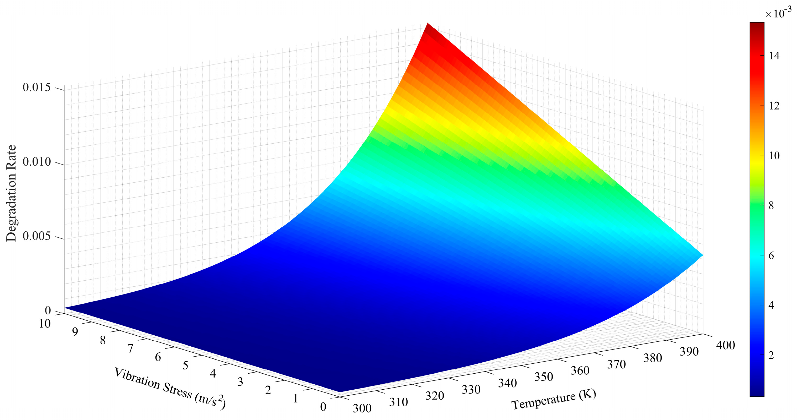
2.2.1. Continuous Degradation Term
2.2.2. Random Interference Term
2.2.3. Random Noise Term
2.2.4. Coupled Degradation Model
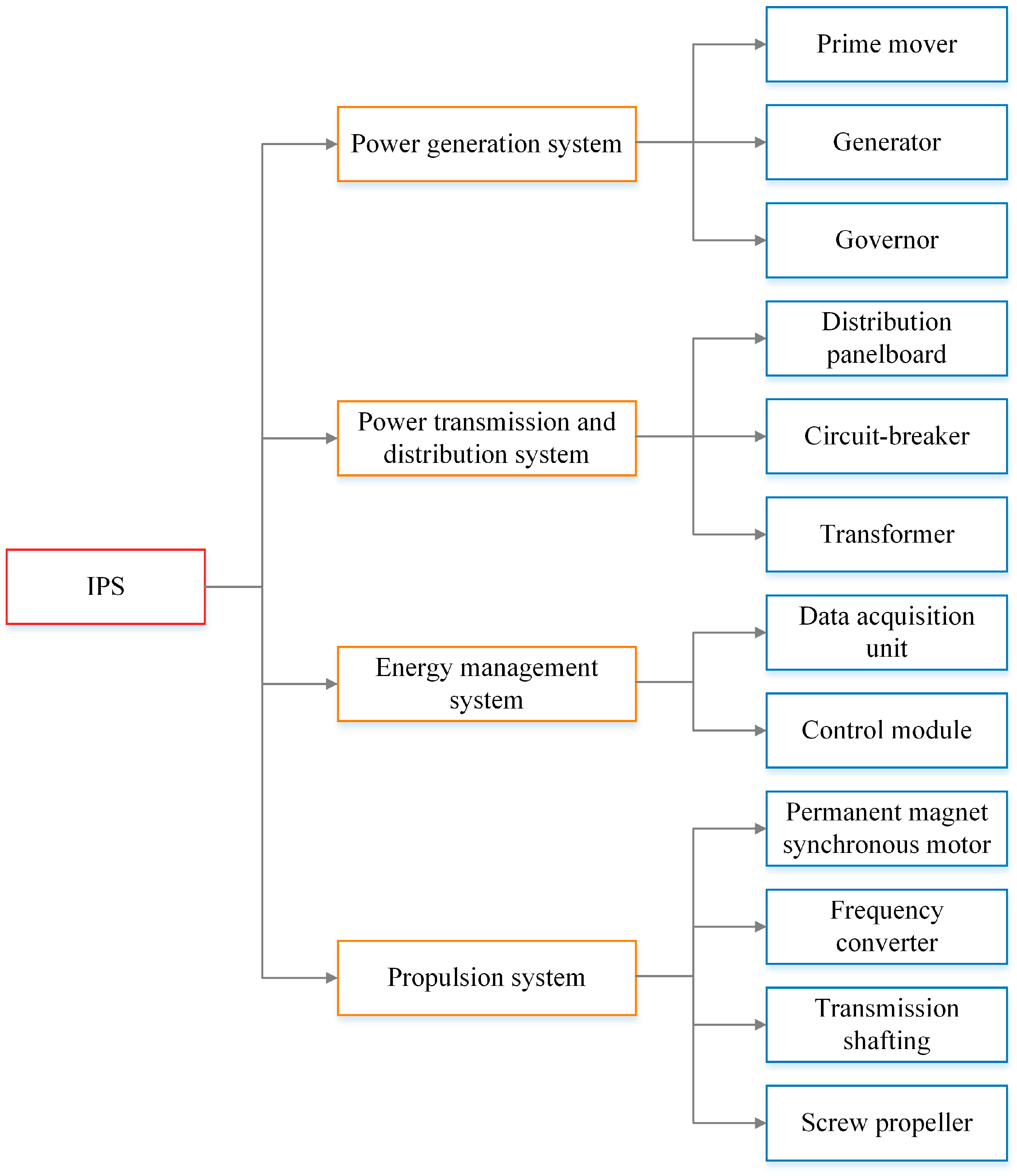
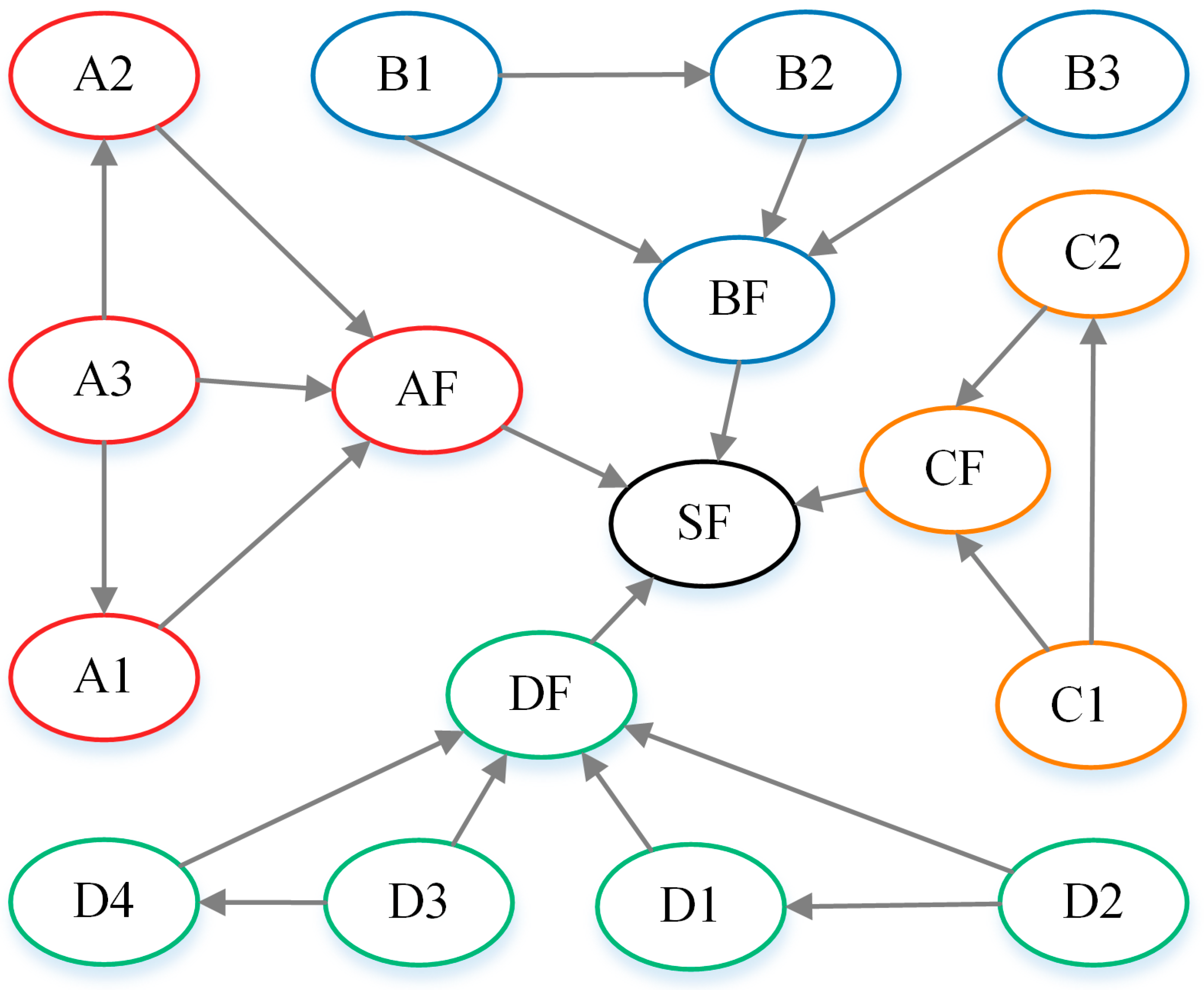
3. System-Level Decomposition and Node Definition
- 1.
- Environment Layer (EL)
- 2.
- Component Layer (CL)
- 3.
- Subsystem Layer (SL)
- 4.
- System Layer (SysL)
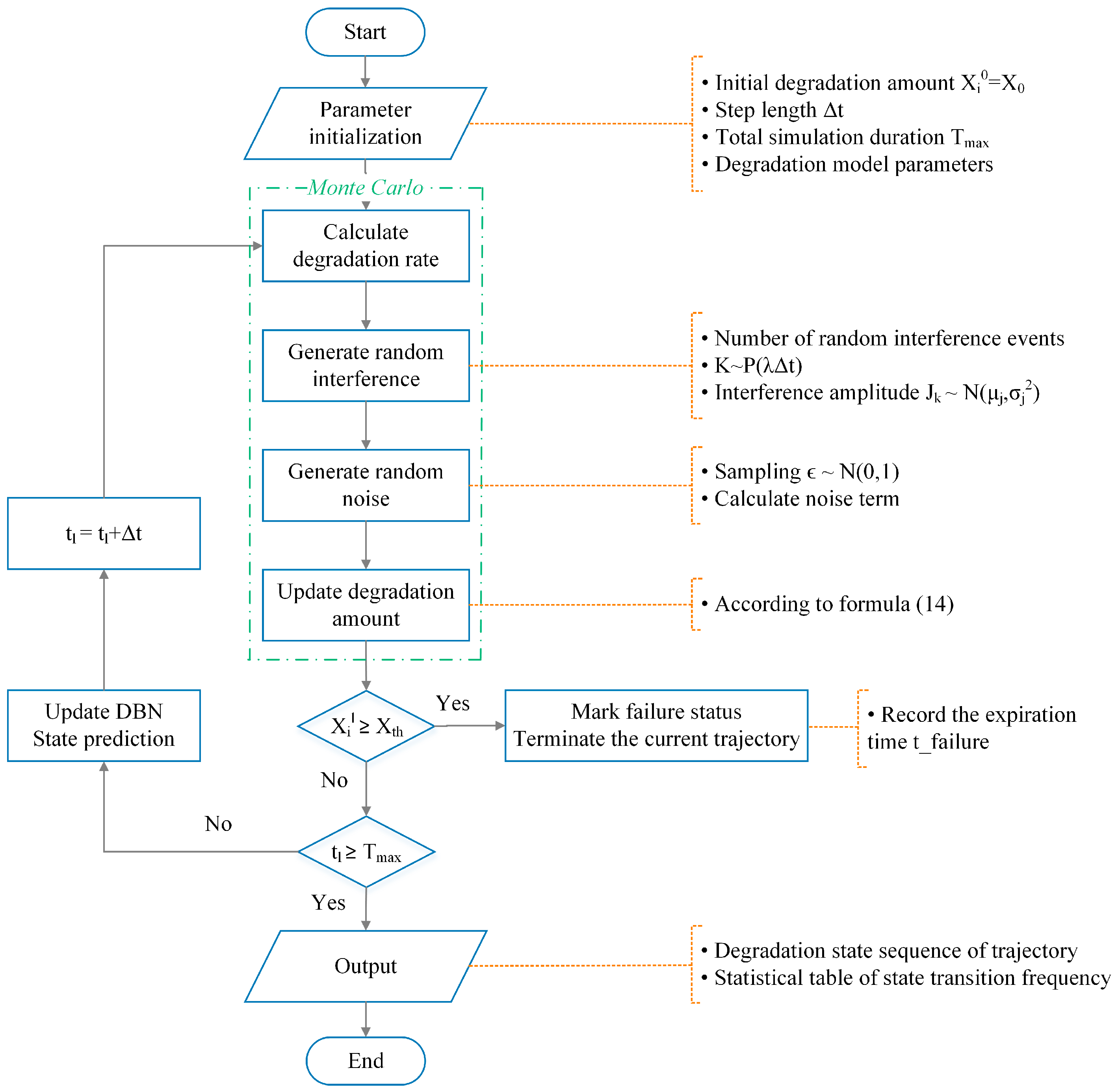
4. Construction of DBN
4.1. Time Slice Design and Dynamic Evolution Rules
4.2. Generation and Update of Conditional Probability Table
- Particle Initialization
- 2.
- State Prediction
- 3.
- Weight Update
- 4.
- Resampling
- 5.
- Parameter Estimation
- Regular update mechanism
- Event triggering mechanism
| Algorithm 1 Particle Filter for CPT Adjustment [30] |
| Input: Prior distribution , Observations , Maintenance parameters , Particle count Output: Posterior estimate , Updated CPT 1: Initialize particles: for = 1 to : // 2: for each time step = 1 to : 3: // State prediction 4: for each particle : 5: ← MCS // Degradation trajectory 6: // Weight update 7: for each particle : 8: // Gaussian likelihood (Equation (16)) 9: // Fuzzy fusion (Equation (17)) 10: // Weight update (Equation (16)) 11: Normalize weights: 12: // Resampling 13: ∼ Uniform [0, 1/] 14: for = 1 to : 15: 16: Select particle with cumulative weight > 17: Reset 18: // Parameter estimation 19: // Posterior estimate (Equation (18)) 20: // CPT update 21: Calculate state transition frequency 22: Normalize → New CPT 23: Update DBN model 24: end for |
5. Case Study
5.1. Case Background and Experimental Design
- Data preprocessing
- 2.
- Dynamic evolutionary simulation
- 3.
- Reliability calculation
- 4.
- Validation design
5.2. Result Analysis
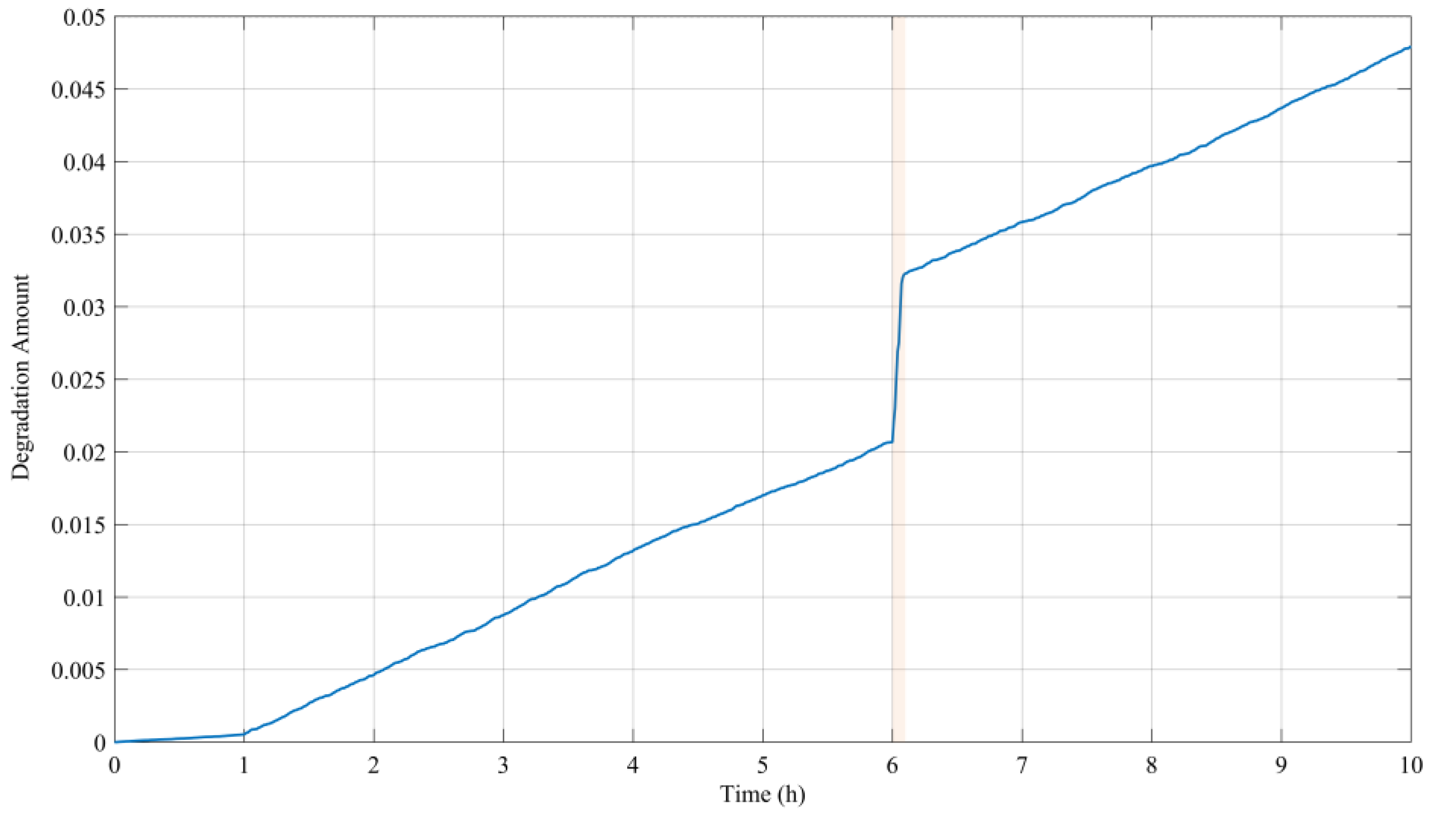
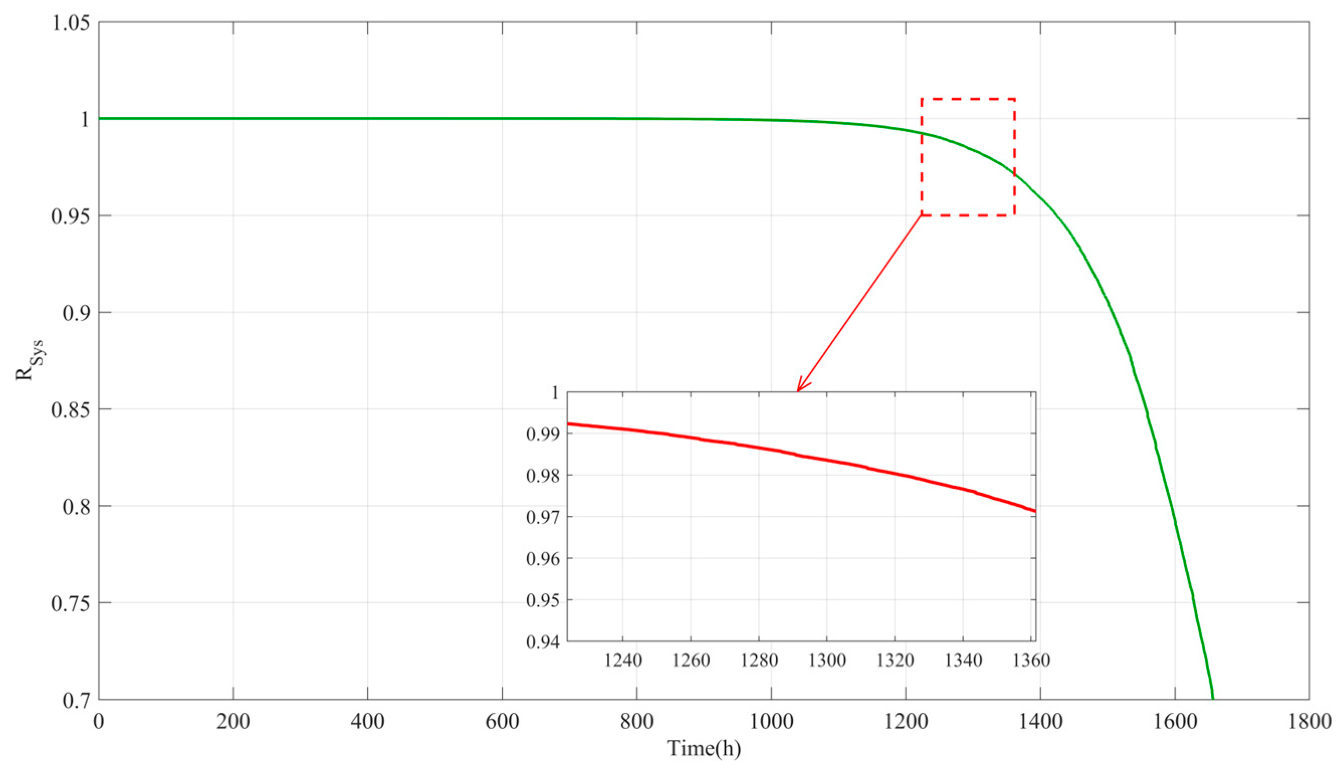
- Initial Stable Stage (0–1000 h)
- 2.
- Initial degradation stage (1000–1200 h)
- 3.
- Accelerated Failure Stage (>1200 h)
6. Conclusions
Author Contributions
Funding
Institutional Review Board Statement
Informed Consent Statement
Data Availability Statement
Conflicts of Interest
Nomenclature
| Symbol | |
| Performance degradation sequence (dimensionless) | |
| Temperature stress sequence (K) | |
| Vibration stress sequence (m/s2) | |
| Random interference process | |
| Random noise process | |
| Temperature stress acceleration coefficient (h−1) | |
| Apparent activation energy (eV) | |
| Boltzmann constant (J/K) | |
| Vibration stress sensitivity coefficient ((m/s2)−1·h−1/2) | |
| Degradation amplitude (dimensionless) | |
| Component layer collection | |
| Subsystem layer components collection | |
| Failure threshold (dimensionless) | |
| Time slicing (h) | |
| Random interference frequency | |
| Greek | |
| Diffusion coefficient (h−1/2) | |
| Vibration enhancement coefficient ((m/s2)−1) | |
| Temperature modulation coefficient (K−1) | |
| Mapping function | |
| Curvature parameter (dimensionless) | |
| Offset parameter (dimensionless) | |
| Tolerance for ambiguity (dimensionless) | |
| SOC switching frequency (h−1) | |
| Abbreviations | |
| IPS | Integrated Power System |
| SOC | System Operating Condition |
| MC | Markov Chain |
| MCS | Monte Carlo Simulation |
| DBN | Dynamic Bayesian Network |
| DTBN | Discrete Time Bayesian Network |
| CTBN | Continuous Time Bayesian Network |
| CPT | Conditional Probability Table |
| MPT | Marginal Probability Table |
| PDFs | Probability Density Functions |
| CL | Component Layer |
| SL | Subsystem Layer |
| SysL | System Layer |
| EL | Environment Layer |
| PL | Particle Filter |
| SBNs | Static Bayesian Networks |
References
- Fang, Z.G. Complex Equipment System Digital Twin; China Machine Press: Beijing, China, 2020. [Google Scholar]
- Wan, Z.B.; Hu, J.G.; Li, J.J.; Chen, L.; Mao, Y.K.; Ye, M.Y. Effectiveness Evaluation of Land-based Intelligent Unmanned Combat Systems Based on Graph Convolutional Networks. Acta Armamentarii 2024, 45, 271–277. [Google Scholar] [CrossRef]
- Gao, Q.; Lu, L.H.; Zhang, R.; Song, L.Y.; Huo, D.H.; Wang, G.L. Investigation on the thermal behavior of an aerostatic spindle system considering multi-physics coupling effect. Int. J. Adv. Manuf. Technol. 2019, 102, 3813–3823. [Google Scholar] [CrossRef]
- Wang, Z.; Hu, Z.Y.; Yang, X.F. Multi-agent and ant colony optimization for ship integrated power system network reconfiguration. J. Syst. Eng. Electron. 2022, 33, 489–496. [Google Scholar] [CrossRef]
- Vizentin, G.; Vukelic, G.; Murawski, L.; Recho, N.; Oeovic, J. Marine Propulsion System Failures-A Review. J. Mar. Sci. Eng. 2020, 8, 662. [Google Scholar] [CrossRef]
- Pan, X.L.; Chen, H.X.; Shen, A.; Zhao, D.D.; Su, X.Y. A Reliability Assessment Method for Complex Systems Based on Non-Homogeneous Markov Processes. Sensors 2024, 24, 3446. [Google Scholar] [CrossRef] [PubMed]
- Kou, L.L.; Chu, B.Q.; Chen, Y.; Qin, y. An Automatic Partition Time-Varying Markov Model for Reliability Evaluation. Appl. Sci. 2022, 12, 5933. [Google Scholar] [CrossRef]
- Li, X.; Wang, L.J. Reliability Assessment of Cyber-physical Distribution System Based on Continuous time Markov Chains. Guangdong Electr. Power 2023, 36, 41–48. [Google Scholar] [CrossRef]
- Shekhar, C.; Devanda, M.; Sharma, K. Reliability analysis of imperfect repair and switching failures: A Bayesian inference and Monte Carlo simulation approach. J. Comput. Appl. Math. 2025, 461, 116–132. [Google Scholar] [CrossRef]
- Ruan, Y.P.; He, Z. Reliability evaluation of complex systems with common cause failures based on dbn-CA. Syst. Eng. Electron. 2013, 35, 900–904. [Google Scholar] [CrossRef]
- Gao, C.; Guo, Y.J.; Zhong, M.J.; Liang, X.F.; Wang, H.D.; Yi, H. Reliability analysis based on dynamic Bayesian networks: A case study of an unmanned surface vessel. Ocean. Eng. 2021, 240, 3514–3529. [Google Scholar] [CrossRef]
- Li, X.; Huang, H.Z.; Huang, P.; Li, Y.F. Reliability Analysis and Fault Diagnosis for Power System via Dynamic Bayesian Network. J. Univ. Electron. Sci. Technol. China 2021, 50, 603–608. [Google Scholar] [CrossRef]
- Huang, C.G.; Huang, H.Z.; Li, Y.F. A bidirectional LSTM prognostics method under multiple operational conditions. IEEE Trans. Ind. Electron. 2019, 66, 8792–8802. [Google Scholar] [CrossRef]
- Peng, W.W.; Li, Y.F.; Yang, Y.J.; Mi, J.H.; Huang, H.Z. Bayesian degradation analysis with inverse Gaussian process models under time-varying degradation rates. IEEE Trans. Reliab. 2017, 66, 84–96. [Google Scholar] [CrossRef]
- Guo, Y.J.; Zhong, M.J.; Gao, C.; Wang, H.D.; Liang, X.F.; Yi, H. A discrete-time Bayesian network approach for reliability analysis of dynamic systems with common cause failures. Reliab. Eng. Syst. Saf. 2021, 216, 1208–1218. [Google Scholar] [CrossRef]
- Huang, T.D.; Xiahou, T.F.; Mi, J.H.; Chen, H.; Huang, H.Z.; Liu, Y. Merging multi-level evidential observations for dynamic reliability assessment of hierarchical multi-state systems: A dynamic Bayesian network approach. Reliab. Eng. Syst. Saf. 2024, 249, 1492–1504. [Google Scholar] [CrossRef]
- Wang, C.; Yuan, S.; Yu, C.; Deng, X.; Chen, Q.F.; Ren, L. Operational reliability analysis of remote operated vehicle based on dynamic Bayesian network synthesis method. J. Risk Reliab. 2025, 239, 162–181. [Google Scholar] [CrossRef]
- Cheng, T.T.; Fan, D.Q.; Liu, X.T.; Wang, J.G. Reliability analysis for manufacturing system of drive shaft based on dynamic Bayesian network. Qual. Reliab. Eng. Int. 2024, 40, 4482–4497. [Google Scholar] [CrossRef]
- Wei, W.T.; Li, M.F.; Zhu, D.H.; Zhong, M.J.; Guo, Y.J.; Du, Z.Y.; Jiang, X.W. Research on Reliability Evaluation Method of Nuclear Energy System Based on Dynamic Bayesian Network. Nucl. Power Eng. 2023, 44, 109–114. [Google Scholar] [CrossRef]
- Li, X.; Li, Y.F.; Li, H.; Huang, H.Z. An algorithm of discrete-time Bayesian network for reliability analysis of multilevel system with warm spare gate. Qual. Reliab. Eng. Int. 2020, 37, 1116–1134. [Google Scholar] [CrossRef]
- Yang, S.Q.; Zeng, Y.; Li, X.; Li, Y.F.; Huang, H.Z. Reliability analysis for wireless communication networks via dynamic Bayesian network. J. Syst. Eng. Electron. 2023, 34, 1368–1374. [Google Scholar] [CrossRef]
- Yao, C.Y.; Han, D.D.; Chen, D.N.; Liu, Y.M. A novel continuous-time dynamic Bayesian network reliability analysis method considering common cause failure. Chin. J. Sci. Instrum. 2022, 43, 174–184. [Google Scholar] [CrossRef]
- Tao, H.H.; Jia, P.; Wang, X.Y.; Wang, L.Q. Reliability analysis of subsea control module based on dynamic Bayesian network and digital twin. Reliab. Eng. Syst. Saf. 2024, 248, 1201–1219. [Google Scholar] [CrossRef]
- Hongseok, K.; Dooyoul, L. An efficient discretization scheme for a dynamic Bayesian network in structural reliability analysis. Proc. Inst. Mech. Eng. 2024, 238, 728–739. [Google Scholar] [CrossRef]
- Zhang, Y.D.; Wang, S.P.; Zio, E.; Zhang, C.; Dui, H.Y.; Chen, R.T. Model-guided system operational reliability assessment based on gradient boosting decision trees and dynamic Bayesian networks. Reliab. Eng. Syst. Saf. 2025, 259, 348–362. [Google Scholar] [CrossRef]
- Wang, Y.Y.; Qian, L.X.; Hong, M.; Li, D.Y. Navigation risk assessment for ocean-going ships in the north pacific ocean based on an improved dynamic Bayesian network model. Ocean. Eng. 2025, 315, 1198–1216. [Google Scholar] [CrossRef]
- Dania, B.H.; Raed, A.; Mohammed, A.; Sa, H. Reliability modeling of the fatigue life of lead-free solder joints at different testing temperatures and load levels using the Arrhenius model. Sci. Rep. 2023, 13, 2493–2505. [Google Scholar] [CrossRef]
- Qu, X.Z. Time-varying reliability analysis of stochastic process discretization method for train traction power impeller vibration. J. Vib. Shock. 2024, 43, 49–60. [Google Scholar] [CrossRef]
- Weber, F.; Wu, H.R.; Starke, P. A new short-time procedure for fatigue life evaluation based on the linear damage accumulation by Palmgren–Miner. Int. J. Fatigue 2023, 172, 1352–1369. [Google Scholar] [CrossRef]
- Yan, X.J.; Zhu, H.M.; Sun, S.Y.; Shi, Z.S.; Jiang, S. A UAV Target Positioning Method Based on Improved Mutant Firefly Algorithm Optimized Particle Filter. Acta Armamentarii 2025, 46, 250459. [Google Scholar] [CrossRef]


| Node Type | Symbolic Representation | Variable Definition |
|---|---|---|
| Degenerate nodes | Degradation of components | |
| Environmental nodes | Environment variable | |
| Reliability nodes | Reliability of the system |
| Node Number | Name | Node Number | Name |
|---|---|---|---|
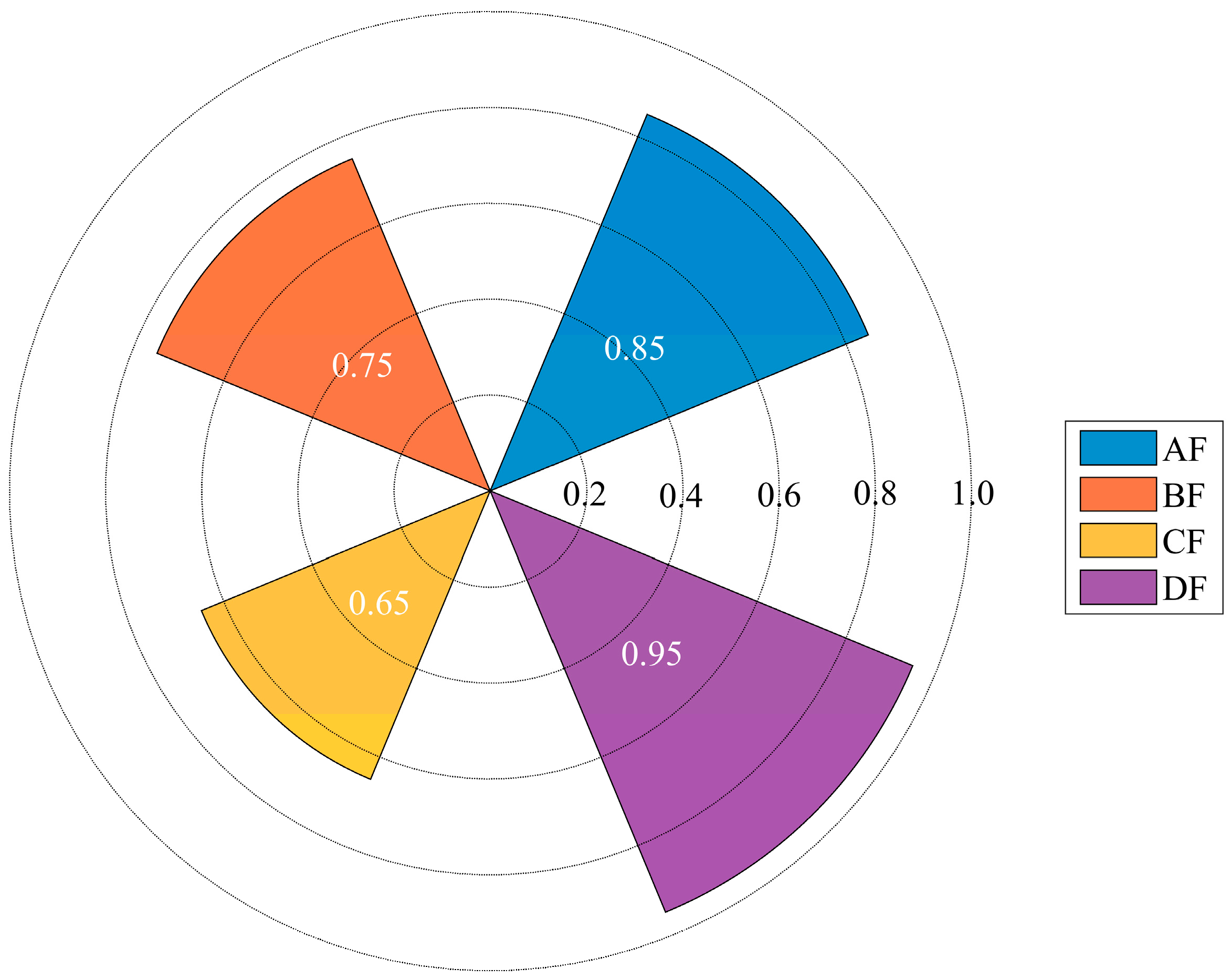
| SF | IPS | B2 | Circuit-breaker |
| AF | Power generation system | B3 | Transformer |
| BF | Power transmission and distribution system | C1 | Data acquisition unit |
| CF | Energy management system | C2 | Control module |
| DF | Propulsion system | D1 | Permanent magnet synchronous motor |
| A1 | Prime mover | D2 | Frequency converter |
| A2 | Generator | D3 | Transmission shafting |
| A3 | Governor | D4 | Screw propeller |
| B1 | Distribution panelboard |
| Parameter | Physical Meaning | Unit | Value Range | Calibration and Verification |
|---|---|---|---|---|
| Temperature stress acceleration coefficient | h−1 | 2.5×10⁻⁴ ± 0.3×10⁻⁴ | 80 °C constant-temperature accel-erated aging tests [27] | |
| Vibration stress sensitivity coefficient | (m/s2)−1·h−1/2 | 1.2×10⁻³ ± 0.2×10⁻³ | Vibration table acceleration test (100 Hz sine vibration) | |
| Apparent activation energy | eV | 0.45 ± 0.05 | Material properties of NdFeB magnets [27] | |
| Vibration enhancement coefficient | (m/s2)−1 | 0.15 ± 0.03 | Dual-stress accelerated tests (100 Hz vibration platform) | |
| Temperature modulation coefficient | K−1 | 0.08 ± 0.01 | Variable-temperature vibration tests (20–120 °C) | |
| Diffusion coefficient | h−1/2 | 0.015 ± 0.002 | Factory test data (100-unit sample) | |
| SOC switching frequency | h−1 | 0.06 ± 0.01 | Warship power system operation logs | |
| Mean degradation amplitude from transient load shocks | Dimensionless | 0.02 ± 0.005 | Sudden load test data [4] | |
| Standard deviation of transient load degradation | Dimensionless | 0.003 ± 0.001 | Failure event statistics | |
| Failure threshold (15% efficiency drop) | Dimensionless | 0.25 ± 0.03 | Historical maintenance records (200 failure cases) |
| Method | Run Time (s) | RMSE vs. MCS |
|---|---|---|
| Proposed DBN | 15.20 | 0.0164 |
| MCS | 85.72 | 0.0000 |
| SBN | 9.54 | 0.0392 |
| MC | 11.37 | 0.0517 |
Disclaimer/Publisher’s Note: The statements, opinions and data contained in all publications are solely those of the individual author(s) and contributor(s) and not of MDPI and/or the editor(s). MDPI and/or the editor(s) disclaim responsibility for any injury to people or property resulting from any ideas, methods, instructions or products referred to in the content. |
© 2025 by the authors. Licensee MDPI, Basel, Switzerland. This article is an open access article distributed under the terms and conditions of the Creative Commons Attribution (CC BY) license (https://creativecommons.org/licenses/by/4.0/).
Share and Cite
Wei, J.; Chen, T.; Wen, H.; Liu, H. Time-Varying Reliability Analysis of Integrated Power System Based on Dynamic Bayesian Network. Systems 2025, 13, 541. https://doi.org/10.3390/systems13070541
Wei J, Chen T, Wen H, Liu H. Time-Varying Reliability Analysis of Integrated Power System Based on Dynamic Bayesian Network. Systems. 2025; 13(7):541. https://doi.org/10.3390/systems13070541
Chicago/Turabian StyleWei, Jiacheng, Tong Chen, Haolin Wen, and Haobang Liu. 2025. "Time-Varying Reliability Analysis of Integrated Power System Based on Dynamic Bayesian Network" Systems 13, no. 7: 541. https://doi.org/10.3390/systems13070541
APA StyleWei, J., Chen, T., Wen, H., & Liu, H. (2025). Time-Varying Reliability Analysis of Integrated Power System Based on Dynamic Bayesian Network. Systems, 13(7), 541. https://doi.org/10.3390/systems13070541