Article

A Game Theoretic Approach to Electric Vehicle Promotion Policy Selection from the Consumer Side

1
School of Management, Wuhan Institute of Technology, Wuhan 430205, China
2
Economics and Management School, Wuhan University, Wuhan 430072, China
*
Authors to whom correspondence should be addressed.
Systems 2025, 13(7), 506; https://doi.org/10.3390/systems13070506
Submission received: 6 May 2025 / Revised: 14 June 2025 / Accepted: 20 June 2025 / Published: 23 June 2025
(This article belongs to the Section Systems Practice in Social Science)

Abstract

With the increasing popularity of electric vehicles (EVs) through purchase subsidy (PS) policies, the personal carbon tax (PCT) policy has been adopted by some countries due to its characteristics of restraining the diffusion of fuel vehicles (FVs) from the consumer side. This paper constructs a three-stage game model consisting of government, manufacturers, and consumers to investigate the impact of basic utility valuation heterogeneity differences on the optimal decisions and to compare the implementation effects of two policies. The results are as follows. First, conventional wisdom suggests that EV consumer surplus under PS policy will exceed that under PCT policy. Surprisingly, our results show that when the basic utility valuation difference is small, the EV consumer surplus under PCT policy exceeds that under PS policy. Second, for manufacturers, it is interesting to note that the sustained impact of PCT policy on promoting the diffusion of the EV market and the profit of the EV manufacturer is related to the basic utility valuation heterogeneity difference. However, compared with PS policy, the implementation of PCT policy has a better restraining effect on the diffusion of the FV market, effectively reducing the demand for FV and the profit of FV manufacturers. Finally, contrary to the common belief that increasing subsidies or raising carbon taxes can increase overall social welfare, this paper shows that subsidies and carbon taxes have a dual impact on overall social welfare, and only when their positive effects outweigh the negative ones can such policies become effective ways of promoting industrial transformation.

1. Introduction

Electric vehicles (EVs) have experienced rapid growth in production and sales as an alternative to traditional fuel vehicles (FVs) in recent years [1,2,3,4]. However, EVs’ market share still exhibits significant differences compared to that of FVs [5]. Based on a comprehensive analysis of sales data from multiple countries, although the sales of EVs are experiencing rapid growth, the sales of FVs still dominate globally. Taking China, one of the world’s largest car markets, as a typical example, the latest data from the Ministry of Public Security, as of the end of 2024, the national stock of EVs stood at 31.4 million units, accounting for only 8.9% of the total number of automobiles. The emergence of this phenomenon may stem from the basic utility valuation heterogeneity between FVs and EVs for consumers.
Comparing FVs and EVs of the same type in the market, it is found that they not only differ in their environmental impact but also in their basic utility valuation as transportation tools, mainly reflected in aspects such as driving range, driving comfort, and appearance. For example, EVs face challenges such as a lack of charging infrastructure, range anxiety, and resale anxiety, which lead to higher upfront purchase costs for EVs [6,7,8]. However, FVs also have issues such as environmental pollution anxiety and fuel anxiety. Therefore, there can be varying levels of basic utility valuation for EVs and FVs of the same type. We refer to such differences as basic utility valuation heterogeneity.
To eliminate barriers to consumer acceptance of EVs, multiple countries’ governments have implemented various incentive policies to promote the development of the EV industry. These policies include purchase subsidies, free license plates, unrestricted access, free parking, and consumer tax credit incentives, among others [9,10,11,12]. The implementation of purchase subsidy (PS) policy is one of the key measures adopted by governments worldwide to promote the development of the EV industry [13,14]. Driven by subsidy policy, consumer willingness to purchase EVs has significantly increased. However, excessive reliance on massive financial support may reduce the competitiveness and sustainability of the EV industry, leading to potential fraud [15,16,17]. In summary, subsidy policy plays a crucial role in promoting the EV industry [18]. However, it is also acknowledged that there are areas for improvement in the implementation of this policy [19]. Therefore, exploring optimal subsidy policies under different market conditions holds significant research value for providing references to other countries globally.
Meanwhile, in promoting the robust development of the EV industry, numerous scholars have proposed various feasible policies beyond the PS policy. Among a series of viable policies like the EV mandate policy [20,21], there seems to be a consensus on the options of personal carbon trading and carbon taxes. For instance, in Norway and Sweden, the government motivates consumer purchase behavior towards EVs and EV manufacturers’ supply to the market by imposing multiple taxes on FV consumers while exempting EV consumers [22]. This policy of personal carbon tax (PCT) implies that the government levies a certain amount of carbon tax on the purchase of FVs, thereby increasing the cost of FVs [23]. Consequently, the challenges and opportunities facing the PCT policy are multifaceted. In this case, maximizing the effectiveness of the PCT policy is a question worth paying attention to.
Inspired by existing policies and research in the field, this paper attempts to contrast the effects of the PS policy with those of the PCT policy and discuss the key issues of implementing both policies using game-theoretic relationships among participants. We provide insights for the government to formulate optimal subsidies and carbon taxes from the perspectives of the market demand, the manufacturers’ profits, and the overall social welfare. The research aims to address the following research questions:
  • What are the optimal decisions for the consumers, the manufacturers, and the government under different levels of EV carbon emissions?
  • In the context of promoting EVs, restraining FVs, reducing environmental pollution, and enhancing social welfare, which policy is more advantageous?
  • How does the basic utility valuation heterogeneity affect the implementation effect of different policies for promoting EVs?
To achieve this goal, the study was conducted following the four steps below. Firstly, apply the PS policy or PCT policy to the vehicle market. Secondly, develop a three-stage Stackelberg game model involving consumers, manufacturers (EV manufacturers and FV manufacturers), and the government. Thirdly, obtain the model’s solution by using backward induction to determine consumer purchase decisions, manufacturers’ pricing decisions, and government subsidy or carbon tax decisions. Finally, discuss the optimal implementation of the PS policy and the PCT policy through numerical simulations and validating the reliability of the model.
Through the above research steps, this paper draws the following conclusions. Firstly, our research finds that blindly increasing subsidies or raising carbon taxes does not always lead to an increase in social welfare. However, compared to the PS policy, adopting the PCT policy can significantly reduce pollution from automobiles. Secondly, our study identifies governmental tendencies in formulating policies for promoting the EV market. Specifically, governments show a preference for adopting proactive measures when the environmental benefits of EVs are pronounced. This includes offering higher subsidy levels or imposing higher carbon taxes. Conversely, in scenarios where the environmental benefits of EVs are less evident, governments may opt for more conservative policies. Thirdly, our research findings indicate that the consumer surplus of EVs under the PS policy is not always higher than the PCT policy. Finally, from the perspective of FV market demand and FV manufacturer’s profit, our analysis shows that compared to the PS policy, the implementation of the PCT policy has a better restraining effect on the diffusion of FV cars in the market. However, from the perspective of EV market demand and EV manufacturer profit, the PCT policy cannot sustainably improve the diffusion of the EV market.
Compared to previous studies, the main innovations of this paper are reflected in the following aspects. First, from the research perspective, this paper breaks away from the traditional focus on enterprise-side policy tools (such as dual credit systems, carbon trading, and infrastructure subsidies) or single consumer subsidies. It systematically constructs a combination of consumer-side policy instruments (including subsidies and carbon tax policies) in relation to the development of the new energy vehicle industry, providing theoretical support for the successful implementation of PS and PCT policies in practice. Second, in model construction, this paper innovatively introduces the coefficient of consumer utility valuation differences as a core variable, systematically examining the impact of different value ranges on policy effects. This expands the boundaries of utility valuation for two types of vehicles in traditional studies and better aligns with consumers’ considerations of basic vehicle utility when making purchasing decisions. Finally, the research conclusions of this paper suggest that the carbon emission level of new energy vehicles is a key regulatory variable for the government to formulate optimal subsidy and carbon tax policies, revealing the dynamic relationship between optimal government decisions and carbon emissions. This provides new ideas for future policy design and further promotes the widespread adoption of new energy vehicles among consumers.
The rest of this paper is organized as follows. Section 2 provides a review of the existing literature. Section 3 describes and establishes the model. Section 4 introduces the subsidy mechanism under the PS policy and subsequently analyzes the optimal subsidy scheme by solving the solution of the model. Section 5 presents the carbon tax mechanism under the PCT policy and then analyzes the optimal carbon tax scheme. Section 6 conducts numerical simulations to compare the implementation effects of two policies and delves into the impact of differences in basic utility valuation. Section 7 offers corresponding conclusions and policy recommendations. The proofs of this paper are provided in Appendix A.

2. Literature Review

There are two streams of research related to this paper: the impact of basic utility heterogeneity differences on automotive supply chain decisions and the effect of the government’s incentive policies on EVs. Next, this section will outline the pertinent literature in our field and highlight the main distinctions between our study and each stream.

2.1. The Impact of Basic Utility Heterogeneity Difference on Automotive Supply Chain Decisions

This article is closely connected to the basic utility heterogeneity, but the existing literature primarily examines the impact of consumer heterogeneity on automotive supply chain decisions. Xie et al. [24] demonstrate that the direction of the impact of the heterogeneity assumption depends on the market positions of high-efficiency vehicles. He et al. [25] studied the influence of consumer heterogeneity on the pricing of automobile enterprises; the results found that environmental concerns may not always stimulate EV sales. Behnood et al. [26] studied the influence of consumer heterogeneity on the acceptance of self-driving cars and found that there are significant differences between the determinants of consumers’ acceptance of partially and fully self-driving cars. Jia and Chen [27] demonstrated that consumer heterogeneous preferences can influence the adoption preferences of plug-in EVs in the automotive supply chain and found that policy effects vary depending on consumer groups and vehicle types.
The above research indicates that consumer behavior, corporation pricing, and government decision-making will all be significantly impacted by consumer heterogeneity. However, they overlook the scenario where the same consumer may value different vehicle types differently. Our paper is differentiated from the above studies by paying attention to the heterogeneity in the basic utility valuation of vehicles themselves and seeking to address this gap.

2.2. The Effect of the Government’s Incentive Policies on EVs

Most of the research on EV incentive policies focuses on those implemented on the enterprise side, such as the dual-credit policy, carbon cap-and-trade policy, and charging infrastructure subsidy policies. For instance, Cheng and Fan [28] explored strategic choices under the dual-credit policy, suggesting that maintaining relatively high credit prices is generally more favorable for promoting the expansion of electric vehicles (EVs). Yi et al. [29] argued that the government can stimulate EV growth and suppress the production of high fuel-consuming vehicles by appropriately adjusting the internal mechanism of the dual-credit policy. Nie et al. [30] found that the carbon cap-and-trade policy is more effective in reducing CO2 emissions compared to the PS policy. Wang et al. [31] showed that carbon trading policies can promote the sustainable development of the automotive industry, but issues like carbon trading pricing mechanisms are key obstacles to implementing carbon trading policies in the automotive sector. Yu et al. [32] conducted a comparative study on the optimal decisions when the government provides charging facility subsidies to different targets, finding that different subsidy schemes can increase the adoption of EVs and enhance consumer welfare. Chen et al. [33] compared charging infrastructure subsidies and consumer subsidies, concluding that the government’s subsidy strategy depends on adoption targets and infrastructure investment costs.
In addition, a small number of scholars have examined the effectiveness of incentive policies implemented on the consumer side, such as consumer subsidies and tax policies. Shao et al. [34] analyzed the effects of consumer subsidy policies and price discount policies, finding that governments tend to prefer offering subsidy incentive programs. Kumar et al. [35] explored four development models of EV subsidies, finding that consumer subsidies provided by the government and investment in charging infrastructure by automakers are the most effective. Srivastava et al. [22] compared optimal decisions under differentiated tax policies and subsidy policies, delving into the implementation effects of four different policy combinations. Liao et al. [36] discussed the game theory relationship between local governments and automakers in the post-subsidy era, suggesting that a phased implementation of carbon tax policies could more stably promote the development of EVs.
It is evident that most literature on government incentive policies focuses on the enterprise side, with limited research on consumer-side incentive policies, and few scholars have conducted comprehensive comparisons of multiple consumer-side policies. Therefore, this paper starts from the consumer-side policy perspective and systematically analyzes the implementation effects of subsidies and tax policies.

2.3. Research Summary

Two key gaps are identified in the existing literature. (1) While many scholars have examined government incentive policies for EVs, there is scarce research discussing government PCT policy for FVs, with limited comparative studies on the efficacy of both policies. (2) The study observes that the discussion on the basic utility valuation heterogeneity difference between the two vehicle types is largely absent in the existing literature, with most studies presuming a higher basic utility valuation for EVs over FVs.
Consequently, given the variations in basic utility heterogeneity between FVs and EVs, more research into the implementation effects of the PS policy and the PCT policy is necessary. Table 1 presents a summary of the current literature, categorized based on basic utility valuation heterogeneity differences, government policies, and other factors.
Compared to relevant studies, this paper makes two main contributions. Firstly, we not only consider the perceived carbon emission differences between EVs and FVs by consumers but also account for differences in their basic utilities, which better aligns with the practical issues consumers face when making decisions. Secondly, the research compares the effects of the PCT policy and the PS policy on market demand, manufacturers’ profits, environmental benefits, and social welfare, providing valuable policy recommendations for the government based on this analysis.

3. Model

3.1. Model Description

Consider a scenario within a competitive market involving an EV manufacturer and an FV manufacturer. Consumers are faced with the choice of purchasing either one of these vehicle types or not buying anything. The government offers two distinct policy options: the PS policy and the PCT policy. Specifically, the PS policy involves the provision of a one-time purchase subsidy (represented as R ) exclusively for consumers who decide to purchase EVs. Conversely, the PCT policy entails the imposition of a single carbon tax (denoted as T ), which is levied upon consumers who decide to purchase FVs.
In this model, we adopt the Stackelberg game [22,30,39] to investigate the decision differences among the government, vehicle manufacturers, and consumers in the automobile market under two policies: the PS policy and the PCT policy. Firstly, the government makes decisions based on the principle of maximizing social welfare by implementing policies, i.e., PS or PCT, and is responsible for policy implementation. Secondly, vehicle manufacturers are responsible for selling vehicles in the market and make optimal decisions on the retail prices of EVs and FVs by predicting potential policies and considering manufacturing costs to maximize their own interests. Finally, consumers make purchase decisions based on the vehicle’s retail price and their driving needs. Consumers’ purchase choices also determine the market demand for both types of vehicles, thereby affecting the pricing strategies of manufacturers and the policy choices of the government. The decision-making process among the three participants is shown in Figure 1. Table 2 summarizes the main parameters and the decision variables of the model.

3.2. Basic Assumption

To fully explore the research problem, this paper proposes the following assumptions:
Assumption 1. 
According to the empirical study by Ashraf et al. [40], there is a significant difference in environmental pollution between EVs and FVs. Additionally, when considering the entire lifecycle, the gap in carbon emissions between pure electric vehicles and hybrid vehicles may not be as large as when only considering the usage phase. We use per-unit carbon emissions to assess the environmental impact of each vehicle throughout its production, transportation, and usage phases. We denote i g as the carbon emission level of the unit FV and i e as the carbon emission level of the unit EV, with i e < i g [22,30,34] .
Assumption 2. 
Assume that the utilities derived from purchasing EVs and FVs, as well as from the decision not to make a purchase by consumers, are as follows:
u e p s = α θ p e + R β i e u g p s = θ p g β i g u e p c t = α θ p e β i e u g p c t = θ p g T β i g u r = 0
Here, we use θ to represent the basic driving utility for consumers (e.g., Nie et al. [30]; Yu et al. [41]; Liu et al. [42]), which follows a uniform distribution on the interval 0 , 1 [34,43,44]. And α represents the coefficient of the basic utility valuation difference between EVs and FVs (including driving range, driving comfort, appearance, and other basic attributes of transportation), with α > 0 and α 1 . According to empirical evidence, α can be classified into two distinct scenarios. When 0 < α < 1 , the willingness to pay for EVs is lower than that for FVs [39]. For example, according to the research by Yang et al. [45], residents in urban areas of Norway, with higher income levels and greater travel demand, tend to prefer EVs. When α > 1 , the willingness to pay for EVs is higher than that for FVs [17]. Similarly, Li et al.’s [46] study shows that in rural areas of China, due to relatively limited consumer income and the need for longer travel distances, people are more inclined to choose FVs. β represents the consumers’ low-carbon preference, with 0 < β < 1 .
Assumption 3. 
Assume that the production cost of FVs is c and the production cost of EVs is k c . By referencing the description of k in Shao et al. [34] and Deng et al. [47], we conclude that k > 1 needs to be satisfied, meaning that the production cost of EVs is higher than that of FVs. And assume manufacturers can independently complete the process of producing and selling vehicles, with the market demand of the two types of vehicles being q e and q g , respectively. Referring to the works of Bao et al. [48] and Han et al. [49] and based on the above discussion, we can summarize the profit expressions of the two types of manufacturers as follows:
π e = p e k c q e π g = p g c q g
Assumption 4. 
Referring to the works of Kumar et al. [35], Varian [50], Bian et al. [51], and Nie et al. [30], the social welfare function comprises four components: consumer surplus, manufacturers’ profits, environmental benefits, and government revenues:
S W = C S + π E S + G
Here, C S represents consumer surplus, comprised of C S e and C S g , which denotes the total utility derived from consumers’ purchases of EVs, FVs, and non-purchase behavior, reflecting consumer satisfaction with their consumption choices. π represents manufacturers’ profits, consisting of π e and π g , representing the sum of profits for the EV manufacturer and the FV manufacturer, respectively. Environmental benefits, represented as E S , refer to the impact of EVs and FVs on environmental pollution during usage and are manifested as the total carbon emissions of both vehicle types. Finally, government revenues, denoted as G , refer to the total investment in consumer subsidies for EVs under the PS policy or the total amount of carbon taxes paid by FV consumers under the PCT policy.
According to the analysis in the previous sections, it is evident that the main difference between the PS policy and PCT policy lies in the behavior of the government and consumers, resulting in differences in consumer utility under these two policies. In the next two sections, the study will individually solve for the optimal decisions of each game player under the two policies and analyze the impacts of purchase subsidies and personal carbon taxes on the internal functioning of the supply chain.

4. PS Policy

In this section, we will use backward induction to solve for the optimal decision of each entity under the PS policy, analyze the impact of different purchase subsidies on social welfare, and explore the optimal choice of purchase subsidies under different carbon emissions. We will discuss α > 1 and α < 1 in the following sections.

4.1. PS ( α > 1 )

As shown in Figure 2, when α is greater than 1, the basic utility valuation of EV is higher than that of FV. Consumers will choose between EV and FV based on their utility comparison. Specifically, when the consumer’s basic driving demand θ is in the range of 0 , θ 2 , there is no purchase behavior. When θ is in the range of θ 2 , θ 1 , the consumer purchases an FV. When θ is in the range of θ 1 , 1 , the consumer purchases an EV. Therefore, we set u e p s = u g p s in Equation (1) to obtain the undifferentiated point θ 1 for consumers to choose between EV and FV. Set u g p s = u r = 0 to obtain the undifferentiated point θ 2 for consumers to choose between FV and no purchase, as shown in Equation (4).
θ 1 p s + = p e p g + β i e β i g R α 1 θ 2 p s + = p g + β i g
According to Shao et al. [34] and Liu et al. [52], it can be concluded that consumers’ purchase behavior directly affects the market demand for automobiles. Therefore, the demand for EVs by consumers is q e p s + = 1 θ 1 , while the demand for FVs is q g p s + = θ 1 θ 2 , as shown in Equation (5). Subsequently, substituting them into Equation (2), we obtain the profit functions for the manufacturers under the PS policy when α is greater than 1, as shown in Equation (5).
q e p s + = 1 + α + R β i e + β i g p e + p g 1 + α q g p s + = R β i e + α β i g p e + α p g 1 α
We then consider the pricing decision of the first follower manufacturers. The solution can be obtained through backward induction.
p e p s + = 1 2 α β i e + α i g β + 2 α k + α c + 2 α 1 R + 2 α α 1 4 α 1 p g p s + = i e β + 1 2 α i g β + 2 α + k c R + α 1 4 α 1 q e p s + = 2 α α 1 2 α 1 i e β + α i g β 2 α k α k c 1 2 α R 4 α 1 α 1 q g p s + = α α 1 + α i e β + α 2 α 2 i g β + α k + α 2 α 2 c α R 4 α 1 α 1
Correspondingly, as observed in Equation (6), the retail prices, the demands, and the profits for EVs are directly proportional to R , while the retail prices, the demand, and the profits for FVs are inversely proportional to R . This result can be explained as follows. The increase in government subsidies for EV consumers reduces their purchasing costs, stimulates consumer demand for EVs, and consequently drives up the retail prices and demand for EVs, leading to increased profits for EV manufacturers. On the other hand, the retail prices and the demand for FVs decrease. Our result provides valuable managerial insights for government management, suggesting that increasing purchase subsidies appropriately can effectively boost EV sales, stimulate consumer purchase behavior towards EVs, promote profit growth for relevant companies, and accelerate the market diffusion of EVs.
Lemma 1. 
Under the PS policy, when α > 1 , given the purchase subsidy R , the relationship between the market demands for both EVs and FVs and the difference in basic utility valuation α is summarized as follows:
(i) 
When 1 2 β i g 2 < c < 1 β i g , then q e and q g would increase as the difference in basic utility valuation α increased.
(ii) 
When 0 < c 1 2 β i g 2
if R m i n < R < R 1 , then q e would increase as the difference in basic utility valuation α increased,
if R 1 R < R m a x , then q e would decrease as the difference in basic utility valuation α increased,
if R m i n < R < R 2 , then q g would increase as the difference in basic utility valuation α increased,
if R 2 R < R m a x , then q g would decrease as the difference in basic utility valuation α increased.
Note: R m i n , R m a x , R 1 , and R 2 are shown in Appendix A.
Through Lemma 1, we can observe that under the given purchase subsidy R , the impact of the difference in basic utility valuation α on the market demands for EVs and FVs exhibits similarities. Interestingly, when the production cost of FVs is lower than a certain critical value, the market demand for both vehicle types does not simply increase with the increase in the difference in basic utility valuation α . However, this contradicts our intuition. This is because the impact of the difference in basic utility valuation α on the market demand for EVs and FVs is influenced by factors such as the production cost of vehicles, carbon emissions from EVs, carbon emissions from FVs, and consumer awareness of low-carbon options, rather than being solely determined by a single factor. Therefore, our conclusion serves as a reference for the future development direction of the automotive industry. Merely focusing on the exclusive development of EVs and expanding the difference in basic utility valuation between EVs and FVs may not necessarily promote the market diffusion of EVs. The direction of automotive research and development should consider multiple factors such as production costs, carbon emissions, and consumer awareness of low-carbon options to drive the common development of multiple vehicle types, including EVs and FVs.
Finally, based on consumers’ purchase behavior and manufacturers’ pricing decisions, the government will make subsidy decisions to maximize social welfare.
S W p s + = α 1 2 θ 1 2 + 1 2 θ 2 2 + α 2 + R p e β i e + π e + π g i e q e i g q g R q e
Proposition 1. 
Under the PS policy, when α > 1 , the marginal effect of government subsidies on social welfare shows non-monotonic characteristics. The direction of this effect is not determined by a single parameter but rather by the interaction between i e and R . The specific variation can be described as follows:
(i) 
When i e i e 2 , the overall social welfare increases with the increase in purchase subsidy.
(ii) 
When i e 2 < i e < i e 1
if R m i n < R < R ^ , then the overall social welfare increases with the increase in purchase subsidy.
If R ^ R < R m a x , then the overall social welfare decreases with the increase in purchase subsidy.
(iii) 
When i e 1 i e , the overall social welfare decreases with the increase in purchase subsidy.
Note: i e 1 , i e 2 , and R ^ are shown in Appendix A.
In reality, most people would intuitively assume that when the government spends a lot of money to provide subsidies to consumers, it would definitely increase social welfare. However, the result of Proposition 1 goes against this intuition. Proposition 1 shows that when i e i e 2 , the government will choose to continuously increase the purchase subsidy to increase the demand for EVs. Although government expenditure will continue to increase, the overall social welfare will increase. When i e 1 i e , the overall social welfare decreases with the increase in purchase subsidy. The environmental benefits brought by purchase subsidy are too small, and the government will not choose to increase purchase subsidy. When i e 2 < i e < i e 1 , if R m i n < R < R ^ , then the overall social welfare increases with the increase in purchase subsidy, and if R ^ R < R m a x , then the overall social welfare decreases with the increase in purchase subsidy.
The explanation for the results of Proposition 1 is as follows. The increase in social welfare is influenced by a combination of consumer surplus, manufacturers’ profits, environmental pollution from automobiles, and government expenditure costs. When subsidies increase, the overall positive effects of increased manufacturers’ profits, consumer surplus, and the environmental impact of FVs contribute to the increase in social welfare. However, the negative effects of government costs and the environmental impact of EVs hinder the increase in social welfare. The trade-off between these opposing effects determines the relationship between social welfare and subsidies. Therefore, purchase subsidies come with costs, and there exists a balance between the costs of subsidy programs and the benefits they bring. Government should vigorously implement subsidy policies only when the positive impacts brought by the subsidy plan outweigh the negative effects.
Proposition 2. 
Under the PS policy, when α > 1 , the optimal decisions for government subsidies and manufacturer pricing are shown in Table 3. It can be observed that i e is a key moderating variable in the decision-making process of supply chain members. The optimal decisions of supply chain members vary depending on different EV carbon emission levels.
In previous studies, Li and Wang [17] argued that it is wise to promote EVs with the maximum subsidy level when their environmental benefits are significant. Interestingly, Proposition 2 reveals that the impact of EV carbon emissions on the optimal purchase subsidy does not exhibit a monotonic trend. Specifically, when i e i e 2 , the optimal purchase subsidy equals R m a x and it decreases with an increase in consumer environmental awareness, increases with the increase in the per-unit carbon emissions of EVs, and decreases with the increase in the per-unit carbon emissions of FVs. When i e 2 < i e < i e 1 , the optimal purchase subsidy increases with an increase in consumer low-carbon awareness, decreases with an increase in the per-unit carbon emissions of EVs, and increases with an increase in the per-unit carbon emissions of FVs. When i e 1 i e , the optimal purchase subsidy equals R m i n , and the relationship between the optimal purchase subsidy and consumer low-carbon awareness is influenced by differences in basic utility valuation and the combined effects of the per-unit carbon emission of EVs and FVs. If 2 α 1 i e > α i g , an increase in consumer low-carbon awareness raises the optimal purchase subsidy; otherwise, it has the opposite effect.
The explanation is shown as follows. When the environmental pollution caused by one EV is smaller than i e 2 , the impact of EVs on environmental pollution is relatively low. With an increase in consumer environmental awareness, purchasing EVs naturally becomes attractive to consumers. Consequently, the government reduces subsidies to minimize fiscal expenditure. However, as EV carbon emissions increase, the attractiveness of EVs compared to FVs diminishes for environmentally conscious consumers. When EV carbon emissions exceed i e 1 , the low-carbon advantage of EVs becomes less pronounced, and consumers need to consider the carbon emissions of both EVs and FVs. Only when the ratio of EV carbon emissions to FV carbon emissions falls within a certain range (i.e., i e > α 2 α 1 i g ) do increasing purchase subsidies influence consumers with low-carbon awareness.

4.2. PS ( α < 1 )

Similar to the situation when α > 1 , this section analyzes the case when α < 1 using backward induction. We first consider the purchasing behavior of the second follower consumers. Unlike the previous scenario, in the case of α < 1 , the basic need valuation for EV is lower than FV, as shown in Figure 3. Consumers still make their choice by comparing the utilities of EV and FV, but the threshold for indifference in consumer purchasing behavior has changed. Specifically, when the consumer’s basic driving need θ 0 , θ 2 , there is no purchasing behavior; when θ θ 2 , θ 1 , the consumer purchases an EV; when θ θ 1 , 1 , the consumer purchases an FV. Therefore, by setting u e p s = u g p s in Equation (1), the study can determine the undifferentiated point θ 1 for consumer indifference between purchasing EVs and FVs. By setting u e p s = u r = 0 , we can determine the undifferentiated point θ 2 for consumer indifference between purchasing an EV and not making any purchase, as shown in Equation (8).
θ 1 p s = p g p e + β i g i e + R 1 α θ 2 p s = p e + β i e R α
Similarly, by using θ to represent the method of expressing automobile market demand, we can determine that consumers’ demand for FVs is q g p s = 1 θ 1 and for EVs is q e p s = θ 1 θ 2 , as shown in Equation (9). Subsequently, substituting them into Equation (2), we can derive the manufacturers’ profit function under the PS policy when α is less than 1, as shown in Equation (9).
q e p s = 1 + α + R β i e + β i g p e + p g 1 + α q g p s = R β i e + α β i g p e + α p g 1 α
Next, let us consider the pricing decisions of the first follower manufacturers. The solution can be obtained through backward induction.
p e p s = α 2 β i e + α i g β + 2 k + α c + 2 α R + α α 2 4 α p g p s = i e β + α 2 i g β + 2 + k c R + 2 2 α 4 α q g p s = 2 1 α + i e β 2 α i g β 2 α k c R 4 α 1 α q e p s = α 1 α + α 2 β i e + α i g β + α k + α 2 k c + 2 α R 4 α 1 α α
Equation (10) indicates that, in the scenario where α is smaller than 1, a rise in purchase subsidies will result in a rise in the retail pricing and the demand for EVs and a fall in those for FVs. This conclusion is the same as when α > 1 . This suggests that the influence of purchase subsidy on EVs’ and FVs’ retail prices and market demand is independent of the coefficient of basic utility valuation difference being larger or less than 1. Our result provides insightful management information for manufacturers. A higher valuation difference between EV and FV is indicated by a difference coefficient greater than 1, which gives the business the option to think about raising prices to boost profitability. In contrast, if α is less than 1, which suggests that there is little to no valuation difference between EVs and FVs, the business might think about reducing the price to draw in more consumers and boost sales volume.
Finally, we consider the leading government’s subsidy decision. Using the same method in Section 4.1, we can obtain the social welfare function, as shown in Equation (11).
S W p s = 1 α 2 θ 1 2 + α 2 θ 2 2 + 1 2 p g β i g + π e + π g i e q e i g q g R q e
Proposition 3. 
Similar to Proposition 1, under the PS policy, when α < 1 , the marginal effect of government subsidies on social welfare also shows non-monotonic changes. The specific variation is as follows:
(i) 
When i e i e 2 , the overall social welfare increases with the increase in purchase subsidy.
(ii) 
When i e 2 < i e < i e 1 ,
if R m i n < R < R ^ , then the overall social welfare increases with the increase in purchase subsidy;
if R ^ R < R m a x , then the overall social welfare decreases with the increase in purchase subsidy.
(iii) 
When i e 1 i e , the overall social welfare decreases with the increase in purchase subsidy.
Note: i e 1 , i e 2 , and R ^ are shown in Appendix A.
Proposition 3 shows that, similar to Proposition 1, increasing purchase subsidies has different impacts on social welfare when the carbon emissions of EVs are at different levels. It indicates that when i e i e 2 , increasing purchase subsidies can increase social welfare. Therefore, the government will choose to increase purchase subsidies to enhance overall social welfare. Conversely, when i e 1 i e , increasing government subsidies will decrease social welfare. When i e 2 < i e < i e 1 and R m i n < R < R ^ , the government will choose to increase purchase subsidies; when R ^ < R < R m a x , the government will choose to reduce purchase subsidies to maximize overall social welfare.
The emergence of this phenomenon is due to the fact that when the carbon emissions of EVs are low, purchase subsidies enable more consumers to purchase and use EVs, reducing the use of traditional FVs and lowering overall carbon emissions. This positive effect on environmental benefits outweighs the negative effect of the expenditure on purchase subsidies, thereby increasing overall social welfare. However, when the carbon emissions of EVs are excessively high, the environmental advantages of EVs compared to FVs are not significant, and their role in reducing environmental pollution is not prominent enough. This conclusion may provide a reasonable explanation for the dual credit policy introduced by the government in China. The dual credit policy forces foreign-invested enterprises and traditional automobile companies to undergo technological transformation, with the aim of reducing or even abandoning research and development on fuel-powered vehicles, expanding research and development on EVs, and constantly reducing carbon emissions from EVs, thereby improving overall social welfare. Therefore, based on previous research conclusions, our study explores the internal mechanism by which changes in purchase subsidies affect the social welfare, promoting theoretical research and practical application in this field.
Proposition 4. 
Under the PS policy, when α < 1 , i e is a key factor influencing the optimal decision-making of supply chain members. The optimal decisions of supply chain members at different EV carbon emission levels are shown in Table 4.
According to research by He et al. [25], the government’s fiscal incentive may change in response to environmental concerns from encouraging the use of EVs to restricting the too flexible strategic pricing practices of businesses. It is interesting to note that our research supports this conclusion. It is evident from Proposition 4 that to encourage EV development, government subsidies do not rise monotonically as EV carbon emissions decline. To be more precise, when i e i e 2 , the optimal purchase subsidy equals R m a x and the ideal purchase subsidy will progressively increase in tandem with the rise in EV carbon emissions. When i e 2 < i e < i e 1 , the optimal purchase subsidy set by the government will decrease with the increase in EV carbon emissions, while the increase in carbon emissions of FVs will lead to an increase in the optimal purchase subsidy. When i e 1 i e , the optimal purchase subsidy equals R m i n and the government will consider the comparison between EVs and FVs. If i e > α 2 α i g , then the government may formulate different subsidy policies based on the actual environmental performance of vehicles to encourage consumers to choose more environmentally friendly vehicles.

5. PCT Policy

In this section, this paper will solve for the optimal decisions of each entity under the PCT policy, using the same method as under the PS policy. We employ backward induction to analyze the impact of different personal carbon taxes on social welfare and explore the optimal selection of personal carbon taxes under different levels of carbon emissions. Similarly, this section discusses α > 1 and α < 1 , respectively.

5.1. PCT ( α > 1 )

We consider the purchase behavior of the second follower consumers. As shown in Figure 2, by letting u e p c t = u g p c t in Equation (1), we can determine the undifferentiated point θ 2 for consumers to purchase EV and FV under the PCT policy. Also, by letting u g p c t = u r = 0 , we can determine the undifferentiated point θ 1 for consumers to purchase FV and forgo purchasing. Substituting the obtained results into Equation (2), we can derive the profit functions for manufacturers under the PCT policy when α is greater than 1, as shown in Equation (12).
θ 1 p c t + = p e p g T β i g i e α 1 θ 2 p c t + = p g + T + β i g q e p c t + = α 1 p e + p g i e i g β + T α 1 q g p c t + = p e p g + ( i e i g ) β + T α 1 p g β i g i g i e T
Furthermore, the manufacturers determine their pricing decisions based on maximizing their own interests. The solution can be obtained through backward induction, as shown in Equation (13).
p e p c t + = 1 2 α β i e + α β i g + 2 α k + α c + α T + 2 α α 1 4 α 1 p g p c t + = β i e + 1 2 α β i g + 2 α + k c + 1 2 α T + α 1 4 α 1 q e p c t + = 2 α α 1 + 1 2 α β i e + α β i g 2 α k α k c + α T 4 α 1 α 1 q g p c t + = α α 1 + α β i e + α 1 2 α β i g + α k + 1 2 α c + α 1 2 α T 4 α 1 α 1
From Equation (13), with the increase in personal carbon tax, the demand for EVs will increase, while the demand for FVs will decrease. This is consistent with the findings of Srivastava et al. [22], who suggest that taxing only FVs would also boost the demand for EVs, thereby weakening the demand for FVs. The explanation for this result is as follows. By imposing a carbon tax on consumers purchasing FVs, the government increases the cost of purchasing these vehicles, thereby stimulating an increase in the demand for EVs. Additionally, from Equation (13), it can be observed that as consumer awareness of low carbon emissions increases, when α i g 2 α 1 i e > 0 , the retail price and market demand of EVs will increase; otherwise, they will decrease. This finding challenges the traditional notion that low-carbon awareness reduces the sales of EVs, as mentioned by Okada et al. [53]. It is evident that for manufacturing companies, relying solely on an increase in consumers’ own low-carbon awareness is insufficient to boost EV sales. Controlling the carbon emissions of FVs and EVs is also essential. The market dissemination of EVs can only be aided by a rise in consumer low-carbon awareness when the carbon emissions of EVs and FVs satisfy specific requirements.
Lemma 2. 
Under the PCT policy, when α > 1 , given the personal tax T , the relationship between the market demands for EVs and FVs and the difference in basic utility valuation α is summarized as follows:
(i) 
When 1 2 β i e 2 k < c < α β i e k , the q e and q g would increase as the difference in basic utility valuation α increased.
(ii) 
When 0 < c 1 2 β i e 2 k
if T m i n < T < T 1 , then an increase in α produces an increase in the q e ,
if T 1 T < T m a x , then an increase in α produces a decrease in the q e ,
if T m i n < T < T 2 , then an increase in α produces an increase in the q g ,
if T 2 T < T m a x , then an increase in α produces a decrease in the q g .
Note: T m i n , T m a x , T 1 , and T 2 are shown in Appendix A.
Through Lemma 2, the study can observe that, similar to Lemma 1, the impact of the basic utility valuation difference α on the market demand for EVs and FVs is similar given a personal carbon tax, denoted as T . Specifically, when the production cost of FVs is below a certain critical value, the market demand for both EVs and FVs exhibits a trend of initially increasing and then decreasing with an increase in α . Conversely, when the production cost of FVs exceeds the critical value, the market demand for both EVs and FVs gradually increases with an increase in α . However, this contradicts our initial assumption that a larger difference in basic utility valuation α would lead to a greater demand for EVs and a smaller demand for FVs. The reason for this phenomenon is also attributed to the combined influence of production costs, carbon emissions of EVs, carbon emissions of FVs, and low-carbon awareness on the impact of α on the demand for EVs and FVs. Therefore, this finding may have significant implications for manufacturers. Manufacturing companies need to recognize that market decisions are often not explained by a single factor. In the pricing decision-making process, they need to consider factors such as consumer preferences for low-carbon emissions, competitors’ pricing strategies, production costs of EVs, and potential government subsidies to avoid overpricing or excessively high production costs.
Finally, based on the maximization of social welfare, the government makes decisions regarding carbon taxation, as shown in Equation (14).
S W p c t + = α 1 2 θ 1 2 + 1 2 θ 2 2 + α 2 i e β p e + π e + π g i e q e i g q g + T q g
Proposition 5. 
Under the PCT policy, when α > 1 , social welfare does not change monotonically with government carbon taxes. In other words, simply reducing carbon taxes does not necessarily lead to an increase in social welfare. The specific variation is as follows:
(i) 
When i e i e 1 , the overall social welfare increases with the increase in personal carbon tax.
(ii) 
When i e 1 < i e < i e 2 ,
if T m i n < T < T ^ , the overall social welfare increases with the increase in personal carbon tax;
if T ^ T < T m a x , the overall social welfare decreases with the increase in personal carbon tax.
(iii) 
When i e 2 i e , the overall social welfare decreases with the increase in personal carbon tax.
Note: i e 1 , i e 2 , and T ^ are shown in Appendix A.
Srivastava et al. [22] argued that when environmental impact is high, the government should increase green taxes on FVs. Intuitively, most people commonly believe that personal carbon taxes should be monotonically related to the environmental impact of cars. When the environmental impact of cars is high, the government can bring greater benefits to society by increasing carbon taxes. However, the results of Proposition 5 contradict this intuition. It suggests that simply increasing carbon taxes does not increase social welfare, meaning that social welfare does not monotonically change with the change in personal carbon taxes but is influenced by various factors such as carbon emissions from EVs. Specifically, when the carbon emissions of EVs are low, i.e., i e i e 1 , the government will choose to increase T to increase social welfare; when the carbon emissions of EVs are high, i.e., i e 2 i e , the government will choose to decrease T to increase social welfare; when i e 1 < i e < i e 2 , if T m i n < T < T ^ , then the government will increase T , and if T ^ < T < T m a x , then the government will decrease T .
The reasons for the phenomenon of Proposition 5 are as follows. Social welfare is influenced by the environmental benefits, government revenue, consumer surplus, and manufacturers’ profits. With the increase in T , environmental benefits and government revenue will increase, which has a positive impact on the improvement of social welfare. However, with the increase in T , consumer surplus and manufacturers’ profits have a negative impact. Similar to the conclusion of Proposition 1, the balance between these two opposing effects determines the relationship between social welfare and personal carbon taxes. It can be seen that simply increasing carbon taxes does not lead to an increase in social welfare but rather has the negative effect. Our conclusion may offer valuable insights for the government in formulating PCT policy. The government needs to weigh the trade-offs among various factors. When considering an increase in personal carbon taxes, it is necessary to balance the relationship between environmental benefits, government revenue enhancement, consumer surplus, and reduction in manufacturers’ profits to ensure the maximization of the policy’s overall effectiveness.
This conclusion may provide a reasonable explanation for the future trend of integrating EVs into the carbon emission trading system. Although the automotive industry currently emits relatively low carbon during the manufacturing process and is not included in the key industries for carbon emission management, our findings suggest that a well-designed PCT policy can enhance social welfare. Additionally, raising carbon taxes within a reasonable range can raise consumer awareness of the economic and environmental value of EVs, thereby adjusting market structure, promoting the adoption and use of EVs, and accelerating the green transformation process. Furthermore, in accordance with the State Council’s Guiding Opinions on “Accelerating the Establishment of a Sound Green, Low-carbon, and Circular Economic Development System” issued in 2021, it is evident that integrating EVs into the carbon emission trading system is a future trend. Therefore, our conclusion predicts and verifies the rationality of future policies in the EV industry, providing valuable insights for subsequent research.
Proposition 6. 
Under the PCT policy, when α > 1 , i e is a key factor influencing the optimal decision-making of supply chain members. The optimal decisions of supply chain members at different EV carbon emission levels are shown in Table 5.
In prior research, it has been mentioned by Srivastava et al. [22] that governments can deter the production or use of vehicles with higher emission rates by imposing higher green taxes. Therefore, intuitively, we would expect carbon taxes levied on FVs to be closely associated with their carbon emissions. Interestingly, Proposition 6 reveals that the carbon emissions of EVs, consumer preferences for low carbon, and differences in basic utility valuation are also closely linked to carbon taxes. Specifically, when i e i e 1 , the optimal carbon tax equals T m a x and as consumer awareness of low carbon increases, personal carbon taxes decrease. Conversely, when i e 1 < i e < i e 2 , as consumer awareness of low carbon increases, personal carbon taxes increase. When i e 2 i e , the optimal carbon tax equals T m i n and the impact of consumer low-carbon awareness on the optimal carbon tax is jointly influenced by EV carbon emissions, FV carbon emissions, and differences in basic utility valuation. When 2 α 1 i e > α i g , an increase in consumers’ low-carbon awareness raises personal carbon taxes. When 2 α 1 i e < α i g , as consumer low-carbon awareness increases, personal carbon taxes decrease.
Similar to Proposition 2, when EV carbon emissions are low, an increase in consumer low-carbon preferences leads to an initiative selection of EVs. At this point, the role of personal carbon taxes is not significant; thus, the government reduces carbon taxes. However, as EV carbon emissions increase, the attractiveness of EVs compared to FVs diminishes for environmentally conscious consumers. Therefore, the government increases the cost of purchasing FVs by increasing carbon taxes to promote the purchase of EVs. However, when EV carbon emissions exceed a certain threshold, the low-carbon advantage of EVs is not pronounced enough, and consumers need to consider the carbon emissions of EVs and FVs. Only when the ratio of EV to FV carbon emissions falls within a certain range do increasing personal carbon taxes effectively influence environmentally conscious consumers.
This conclusion also provides practical insights for vehicle manufacturing companies. Manufacturers must fully consider the impact of environmental factors on policy formulation and implementation and should commit to technological innovation to drive the research and production of EVs and other low-carbon vehicle models, adapting to adjustments in government PCT policy and changes in market demand. This signifies that companies need to increase investment in EV technologies and enhance the performance, range, and accessibility of charging facilities for EVs to meet consumer preferences for low-carbon and environmental awareness. Bunsen et al. [54] noted that many countries, such as India and France, have increasingly implemented stringent tailpipe emission regulations to achieve zero-emission or low-emission vehicles. Our research findings may offer a rational explanation for this trend. The rigorous enforcement of tailpipe emission regulations by these countries represents a policy choice made after considering various factors such as environmental impact, consumer low-carbon preferences, and industrial development. Their aim is to maximize societal welfare and environmental benefits. Therefore, by promoting the development and adoption of EVs, these countries seek to reduce air pollution, improve public health, and create a more sustainable transportation system for the future.

5.2. PCT ( α < 1 )

Next, we consider the case where α < 1 and similarly employ backward induction for the solution. First, we examine the purchase behavior of the second follower consumers. As illustrated in Figure 3, setting u e p c t = u g p c t in Equation (1), we can determine the undifferentiated point θ 1 at which consumers are indifferent between purchasing EVs and FVs under the PCT policy. By setting u e p c t = u r = 0 , we ascertain the undifferentiated point θ 2 at which consumers are indifferent between purchasing EVs and abstaining from purchase. Substituting the obtained results into Equation (2), we derive the profit function of manufacturers under the PCT policy when α < 1 , as shown in Equation (15).
θ 1 p c t = p g p e + i g i e T + β 1 α θ 2 p c t = p e + β i e α q e p c t = p g p e + i g i e T + β 1 α p e + β i e α q g p c t = 1 α p g + p e i g i e T + β 1 α
Subsequently, the manufacturers determine their pricing decisions based on maximizing their own interests. The solution can be obtained through backward induction, as shown in Equation (16).
p e p c t = α 2 β i e + α β i g + 2 k + α c + α T + α α 2 4 α p g p c t = β i e + α 2 β i g + 2 + k c + α 2 T + 2 2 α 4 α q e p c t = α 1 α + α 2 β i e + α β i g + α k + α 2 k c + α T 4 α 1 α α q g p c t = 2 2 α + β i e + α 2 β i g 2 α k c + α 2 T 4 α 1 α
Equation (16) indicates that, when α is less than 1, an increase in PCT will lead to a rise in EV retail prices and demand, while causing α decrease in FV retail prices and demand. This finding aligns with the variation observed under PCT policy where α is greater than 1. It suggests that the impact of PCT on EV and FV retail prices and market demand is independent of whether the coefficient of basic utility valuation difference α is greater than or less than 1. However, unlike the scenario where α is greater than 1, with an increase in consumer low-carbon awareness, when α i g 2 α i e > 0 , EV retail prices and sales will increase; otherwise, they will decrease. This indicates that variations in α being greater than or less than 1 affect the critical value between consumer low-carbon awareness and changes in EV retail prices and demand. This finding underscores the importance of the coefficient of basic valuation difference for manufacturers’ pricing decisions. For manufacturing enterprises, understanding the critical value is crucial for formulating effective market strategies, observing changes in consumer basic utility valuation differences, low-carbon preferences, and other factors; identifying critical values through market research and data analysis; and making appropriate decisions to ensure the company maintains a competitive advantage in a fiercely competitive market environment. Through the analysis of the PCT policy and the PS policy in both scenarios, the study can conclude that regardless of the level of difference in consumer valuation of basic valuation, both the PCT policy and the PS policy can effectively stimulate consumer demand for EVs while reducing demand for FVs.
Finally, we consider the leading government’s carbon taxation decision. Using the same method in Section 4.1, we obtain the social welfare function, as shown in Equation (17).
S W p c t = 1 α 2 θ 1 2 + α 2 θ 2 2 + 1 2 β i g T p g + π e + π g i e q e i g q g + T q e
Proposition 7. 
Under the PCT policy, when α < 1 , social welfare does not change monotonically with government carbon taxes. In other words, simply reducing carbon taxes does not necessarily lead to an increase in social welfare. The specific variation is as follows:
(i) 
When i e i e 1 , the overall social welfare increases with the increase in T .
(ii) 
When i e 1 < i e < i e 2 ,
if T m i n < T < T ^ , then the overall social welfare increases with the increase in T ;
if T ^ T < T m a x , then the overall social welfare decreases with the increase in T
(iii) 
When i e 2 i e , the overall social welfare decreases with the increase in T .
Note: i e 1 , i e 2 , and T ^  are shown in Appendix A.
In existing research, scholars have investigated the impact of EV carbon emission levels and FV carbon emission levels on social welfare. For instance, Srivastava et al. [22] demonstrated that the government needs to utilize carbon taxes to maintain EV carbon emissions at lower levels and FV carbon emissions at moderate levels to maximize social welfare. Interestingly, our findings precisely validate this conclusion. Proposition 7 shows that when EV carbon emissions are less than i e 1 , social welfare is positively correlated with T . When EV carbon emissions exceed i e 2 , social welfare is inversely proportional to T . When EV carbon emissions are between i e 1 and i e 2 , social welfare increases with T within the range of T m i n < T < T ^ , but decreases with T within the range of T ^ < T < T m a x . The interpretation of this phenomenon is similar to the case where α > 1 . The combined effects of the environmental benefits of cars, government revenue, consumer surplus, and manufacturers’ profits contribute to the emergence of this phenomenon.
Compared to studies that focus on the impact of EV carbon emissions and FV carbon emissions on social welfare by Srivastava et al. [22], we choose to explore the trends of their effects on social welfare from the perspectives of EV carbon emissions and personal carbon taxes. This approach offers a more detailed and comprehensive analysis because personal carbon taxes directly influence consumer purchase behavior towards EVs, while EV carbon emissions are one of the key factors in this process. By examining from these two angles, we can intuitively understand the relationship between carbon emissions and social welfare and can promote EV consumption through policy measures such as adjusting personal carbon taxes, thereby not only increasing EV sales but also contributing to the enhancement of social welfare. In summary, our study not only highlights the impact of personal carbon taxes and EV carbon emissions on social welfare but also provides some reference for vehicle manufacturers to control vehicle carbon emissions to promote EV sales and offers practical suggestions for governments to formulate relevant carbon tax policies based on existing vehicle carbon emission levels.
Proposition 8. 
Under the PCT policy, when α < 1 , i e is a key factor influencing the optimal decision-making of supply chain members. The optimal decisions of supply chain members at different EV carbon emission levels are shown in Table 6.
Through the analysis of Proposition 6, we have identified the variations between consumer low-carbon preferences and personal carbon taxes under the PCT policy when α is greater than 1. Therefore, we can anticipate that when α is less than 1, similar variations in these aspects might occur. Unexpectedly, when the EV carbon emissions are between i e 1 and i e 2 , divergent changes emerge. Specifically, when i e i e 1 , the optimal carbon tax equals T m a x and as consumer low-carbon consciousness increases, personal carbon taxes decrease. Conversely, when i e 1 < i e < i e 2 , the relationship between the consumer’s low-carbon preferences and the personal carbon taxes is jointly influenced by EV carbon emissions, FV carbon emissions, and the basic utility valuation difference. When 4 + α 2 3 α i g > 4 2 α i e , as consumer low-carbon consciousness increases, personal carbon taxes increase; otherwise, the reverse is true. When i e 2 i e , the optimal carbon tax equals T m i n . Personal carbon taxes within the range of 2 α i e α i g > 0 will increase with the rise of consumer preference for low-carbon options, while within the range of 2 α i e α i g < 0 , the increase will be comparatively smaller as consumer preference for low-carbon options increases.
The underlying reasons for this discrepancy are as follows. When EV carbon emissions are low, consumers with strong low-carbon preferences proactively opt for EVs, rendering the impact of carbon taxes less pronounced, and hence, the government refrains from imposing high carbon taxes. Since the coefficient of basic utility valuation difference is less than 1, indicating that consumer preferences for EVs relative to FVs are not significant, as EV carbon emissions increase, the advantage of EVs over FVs becomes less apparent. Consequently, consumers consider the carbon emissions of both EVs and FVs. Only within a certain range of the ratio of EV to FV carbon emissions does the method of increasing personal carbon taxes affect consumers with low-carbon consciousness positively. The conclusion of Proposition 8 emphasizes the significance of the coefficient of basic utility valuation difference. Based on this conclusion, the research can provide some insights into the formulation of government PCT policy. For instance, some consumers may prioritize environmental sustainability and be willing to pay a premium for EVs, while others may focus more on price and performance and be less sensitive to carbon emissions.
This finding may resonate with the news reported by The Washington Post in 2021, stating that “General Motors pledges to phase out traditional FVs entirely by 2035 and invest heavily in the development and production of electric vehicles” [32]. This move indicates a growing trend towards transformation in the automotive industry, with EVs poised to become mainstream. Consequently, consumer demand for environmentally friendly and sustainable products is expected to rise, with consumers increasingly willing to pay higher prices for EVs. Therefore, this initiative is expected to stimulate the growth in consumer demand for EVs and accelerate market acceptance of environmentally friendly products. When formulating PCT policy, governments should take this trend into account and develop differentiated carbon tax policies based on the differing needs of consumer groups to better incentivize environmentally conscious consumers to purchase EVs and promote the development of a low-carbon economy.
Proposition 9. 
In four different scenarios, when i e is at a lower level, the optimal subsidy and the optimal carbon tax are R m a x and T m a x , respectively. When i e is at a higher level, the optimal subsidy and the optimal carbon tax are R m i n and T m i n , respectively.
Through the analysis of Propositions 2, 4, 6, and 8, the study observes that in four different scenarios, when i e is at a lower level, the optimal subsidy and optimal carbon tax are both maximized. Conversely, when i e is at a higher level, the optimal subsidy and optimal carbon tax are minimized. This finding reveals a tendency in government policymaking towards promoting the EV market. Only when the environmental benefits of EVs are significant does the government lean towards taking proactive measures, such as providing higher subsidies or imposing higher carbon taxes, to stimulate the growth in demand for EVs. When the environmental benefits of EVs are not as pronounced, the government’s attitude towards policy measures tends to be more conservative, only willing to offer minimal subsidies or implement lower carbon taxes.
Proposition 9 serves as a reminder to relevant automotive companies that they should recognize the importance of technological innovation in enhancing the environmental benefits of EVs. These companies should focus on the emissions and energy efficiency issues of EVs, aiming to reduce carbon emissions and energy consumption during vehicle usage through technological innovation. This approach not only contributes to enhancing the environmental benefits of EVs but also aligns with the government’s requirements for environmental protection and energy conservation, increasing the likelihood of the government implementing proactive incentive measures to collectively promote the healthy development of the electric vehicle market. In addition, automotive companies should actively communicate and collaborate with the government to understand policy trends and market demands, enabling them to adjust their research and development directions and market strategies promptly.

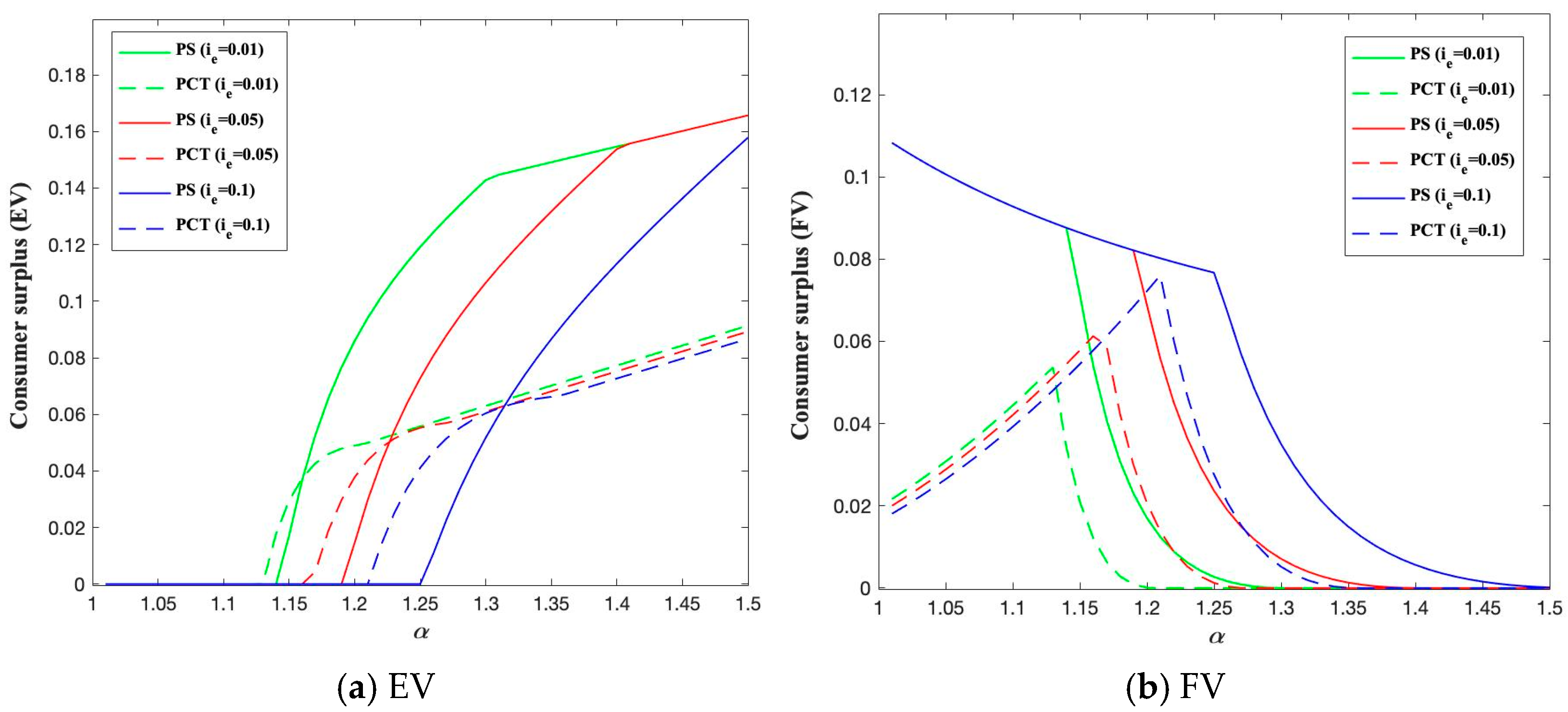
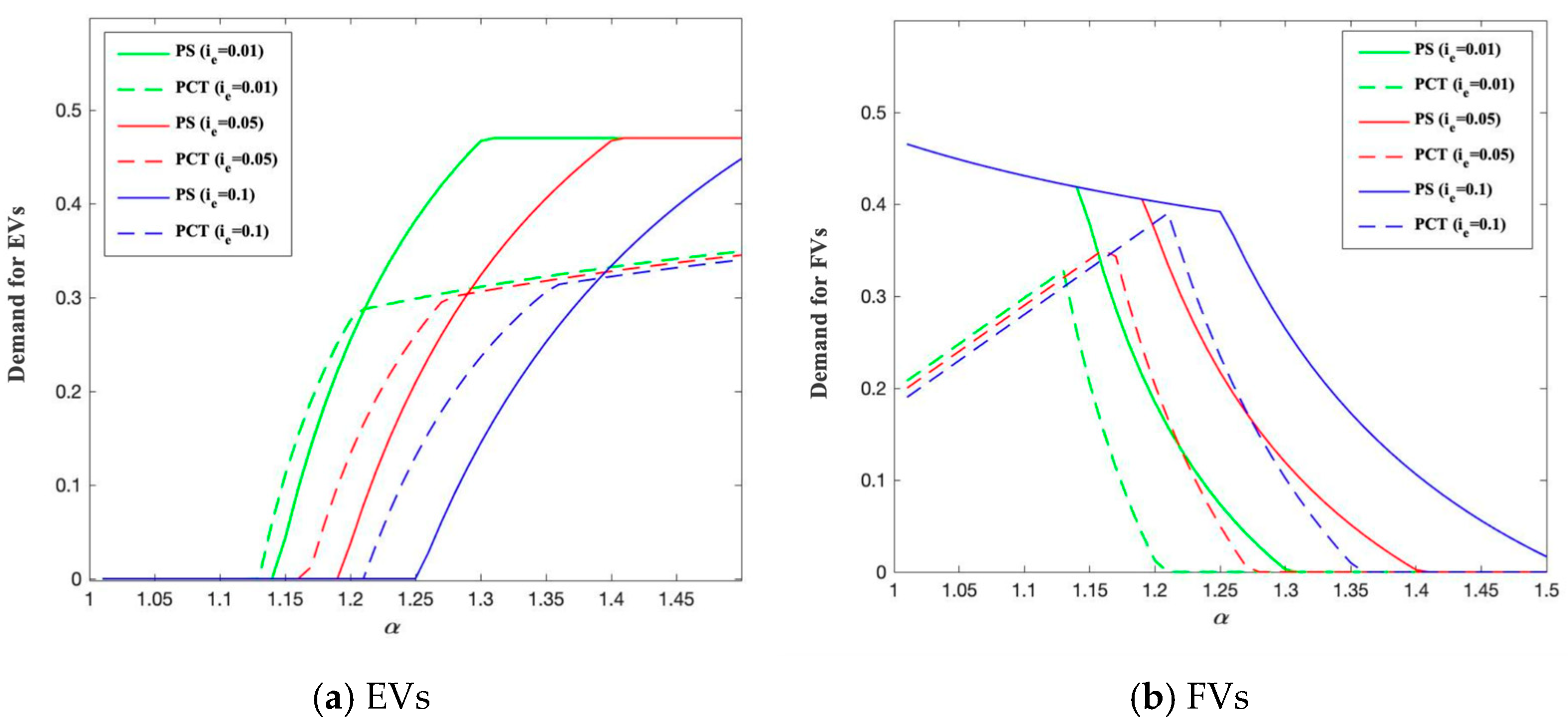
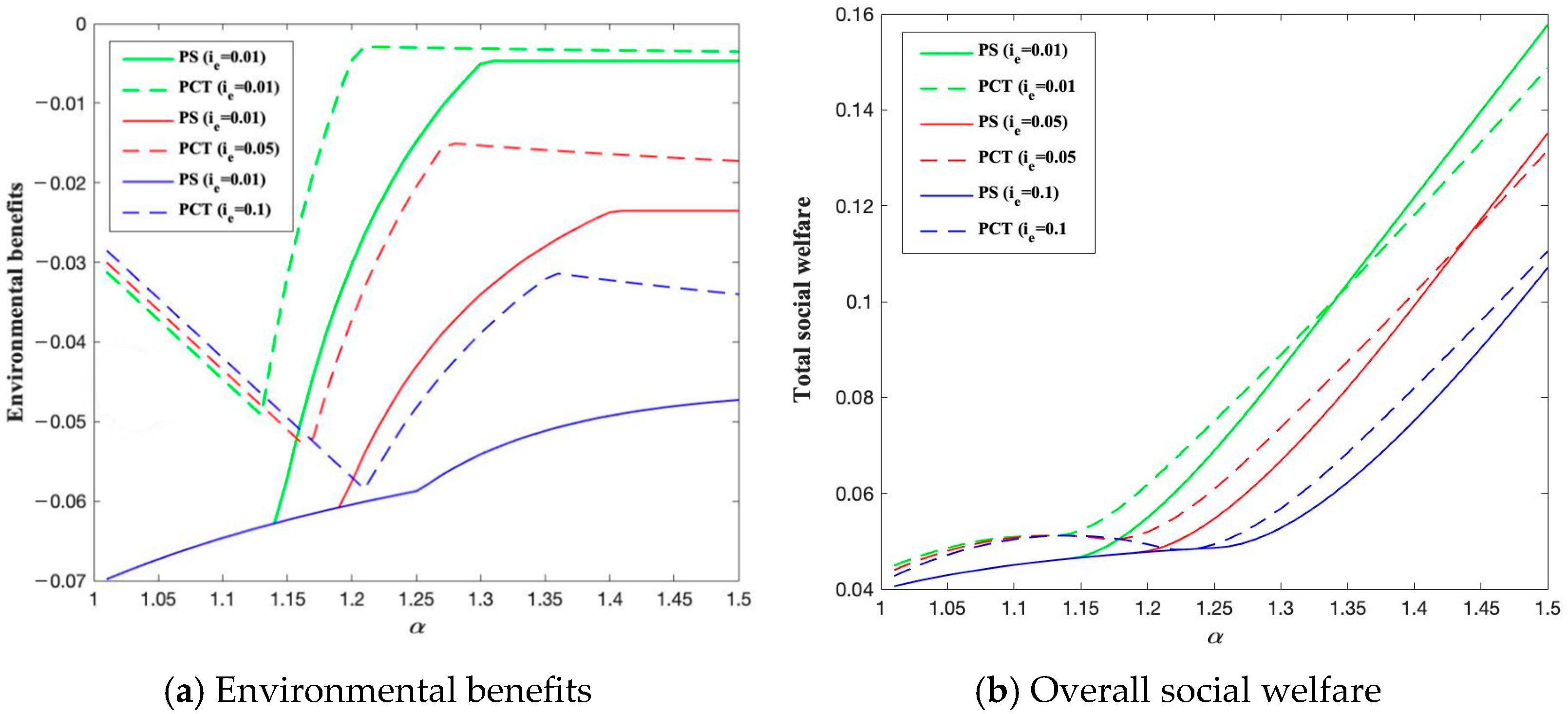
6. Numerical Simulations

In this section, we will further analyze the comparison and analysis of different policies under two contexts through numerical simulations. This section uses MATLAB 2018a to perform corresponding numerical experiments, and the experimental results are as follows.

6.1. Comparison of PCT and PS When α > 1

First, we analyze the impact of differences in basic utility valuation and per-unit carbon emission on different policies, consumer surplus, demands for EVs and FVs, EV manufacturer profit, FV manufacturer profit, environmental benefits, and overall social welfare under α > 1 . The parameter values we have selected satisfy the feasibility conditions under this scenario, with the following specifications:
(1)
We first standardize the model parameters. Assuming that the market size is standardized to 1, we proportionally map key parameters such as unit production costs, unit environmental impact, and market retail prices for both FV and EV to the range [0, 1]. According to the latest data from the Chinese Ministry of Public Security and the China Association of Automobile Manufacturers, the total number of vehicles in China reached 353 million in 2024, with over 260 million passenger cars. The regional distribution shows significant differences: developed coastal areas have a higher penetration rate of private cars, with, for example, 72 private cars per 100 households in urban Zhejiang, while Sichuan has only 32 per 100 households. Based on these data patterns, we set the consumer value acceptance threshold range to [0.32, 0.72]. Since c is lower than p e , and p e does not exceed the average consumer valuation, we select c = 0.5 as the baseline production cost parameter, which is the median of the preset range and well represents the industry’s average cost level.
(2)
Regarding the setting of the production cost coefficient, based on the research of Nie et al. [30] and Deng et al. [47], the unit production costs of EVs and FVs are approximately USD 29,000 and USD 25,000, respectively. According to the 2025 industry report by Eletra Consulting (https://www.go-electra.com/es/, (accessed on 22 June 2025)), as the scale production effect of EVs becomes more apparent, the current production cost of EVs is about 1.1 to 1.7 times that of FVs. Based on this, we set the production cost coefficient under the PS policy to 1.6 and under the PCT policy to 1.1, considering the cost differences in extreme cases.
(3)
Environmental pollution is calculated using a life cycle analysis method. Based on the research by Cen et al. [55] and Shao et al. [34], the exhaust pollution control cost of traditional fuel vehicles is approximately USD 0.01 per mile. Assuming the vehicle scrap mileage is 600,000 miles, the pollution control cost during the usage phase reaches USD 6000. Adding the disposal cost of USD 1430, as estimated by Crane and Mao [56], the total environmental management cost for a fuel vehicle over its entire life cycle is USD 7430. After standardization, i g is set to 0.15, which accurately reflects the relative environmental impact of the vehicle usage phase.
(4)
The United Nations “Global Sustainable Development Report” points out that 60% of Chinese consumers prefer to buy low-carbon emission vehicles and are willing to pay an additional 5–10% for environmentally friendly products and services (https://sdgs.un.org/zh/gsdr, (accessed on 22 June 2025)). It can be reasonably inferred that, in the car-buying decision process, the weight of the low-carbon factor is lower than the price factor but still has a significant influence. Based on the research of Shao et al. [34] and Nie et al. [30], we set β to 0.2.
Figure 4 illustrates the change in consumer surplus for purchasing two types of vehicles under different scenarios of basic utility valuation. Interestingly, as shown in Figure 4a, the consumer surplus of EVs under the PS policy is not always higher than that under the PCT policy, contrary to our common belief. This may be because although the subsidies of the PS policy can increase consumer surplus, the effect of this increase is limited and depends on the amount of the subsidy. Therefore, when the difference in basic utility valuation is small, the difference between the two types of vehicles is also small, and the negative impact of the PCT policy (increased cost of FVs) may be more significant than the positive impact of the PS policy (providing subsidies for EVs). Even without subsidies, consumers tend to choose EVs to avoid paying additional carbon taxes. Thus, the PCT policy increases the relative attractiveness of EVs, resulting in a higher consumer surplus for those who purchase EVs under this policy than under the PS policy. However, as shown in Figure 4b, this corresponds to our intuition that the FV consumer surplus under the PS policy is always higher than that under the PCT policy, regardless of the level of the coefficient of variation in the basic utility valuation. This is because the carbon tax increases the purchase cost of FVs, thereby reducing consumer surplus. Under the PS policy, the price of FV remains unchanged, and thus consumer surplus is not directly affected.
Figure 5 depicts the variations in market demand for two vehicle types under different coefficients of difference in basic utility valuation. Specifically, from Figure 5a it can be observed that, under this parameter setting, while holding other conditions constant, the demand for EVs under both policies is directly proportional to the coefficient of difference in basic utility valuation and inversely proportional to EV carbon emissions. This confirms the conclusions drawn in Lemmas 1 and 2, where, within a certain range, the demand for EVs increases with an increase in the coefficient of difference in basic utility valuation. Contrasting the PCT policy with the PS policy, it is found that when the coefficient of difference in basic utility valuation is small, the demand for EVs under the PCT policy is higher than under the PS policy, whereas the opposite is true when the coefficient of difference is large. This finding validates the substitutive effect of the PCT policy for the PS policy under certain conditions. From Figure 5b, it can be seen that, under the given parameter settings, while holding other conditions constant, the demand for FVs under the PS policy is inversely proportional to the coefficient of difference in basic utility valuation and directly proportional to EV carbon emissions. However, under the PCT policy, the demand for FVs initially increases and then decreases as the coefficient of difference in basic utility valuation increases.
Figure 6 illustrates the impact of varying coefficients of difference in basic utility valuation under two policies on the profits of two types of vehicle manufacturers. From Figure 6a, it can be observed that under both policies, the profit of EV manufacturers increases with the rising difference in basic utility valuation and decreases with the increase in EV carbon emissions. Figure 6b reveals that under both policies, the profit of FV manufacturers exhibits a pattern of initially increasing and then decreasing with the increase in the difference in basic utility valuation. Interestingly, under the PS policy, the profit of FV manufacturers increases with the increase in EV carbon emissions, whereas under the PCT policy, when the difference in basic utility valuation is low, the profit of FV manufacturers decreases with the increase in EV carbon emissions, and when the difference in basic utility valuation is high, the profit of FV manufacturers increases with the increase in EV carbon emissions. By comparing Figure 6a,b, the following findings can be made: First, when the difference in basic utility valuation is small, the profits of EV manufacturers under the PCT policy are higher than those under the PS policy, whereas when the difference in basic utility valuation is large, the profits of EV manufacturers under the PS policy are higher. Interestingly, regardless of the level of difference in basic utility valuation, the profits of FV manufacturers under the PS policy are consistently higher than those under the PCT policy.
Figure 7a illustrates the variation in environmental benefits under different policies. Consistent with expectations, compared to the PS policy, the adoption of the PCT policy by the government can effectively mitigate the impact of the transportation industry on environmental benefits. Specifically, under the PS policy, as the difference in basic utility valuation increases, the negative impact on the environment decreases, while the increase in EV carbon emissions leads to a greater negative impact on the environment. Under the PCT policy, when the difference in basic utility valuation is low, the increase in EV carbon emissions results in a smaller negative impact on the environment, whereas when the difference in basic utility valuation is high, the increase in EV carbon emissions leads to an increased negative impact on the environment.
Figure 7b shows the variation in overall social welfare under different policies. Propositions 2 and 6 indicate that the optimal policy choice by the government is influenced by both the difference in basic utility valuation and the carbon emissions of EVs. With other conditions unchanged, when the difference in basic utility valuation is low, the overall social welfare under the PCT policy is higher than that under the PS policy, whereas when the difference in basic utility valuation is high, the overall social welfare under the PS policy is higher than that under the PCT policy. Additionally, as EV carbon emissions continue to increase, the government is more inclined to choose the PCT policy. Consistent with Propositions 2 and 6, this finding from the perspective of social welfare validates the effective substitution effect of the PCT policy for the PS policy.

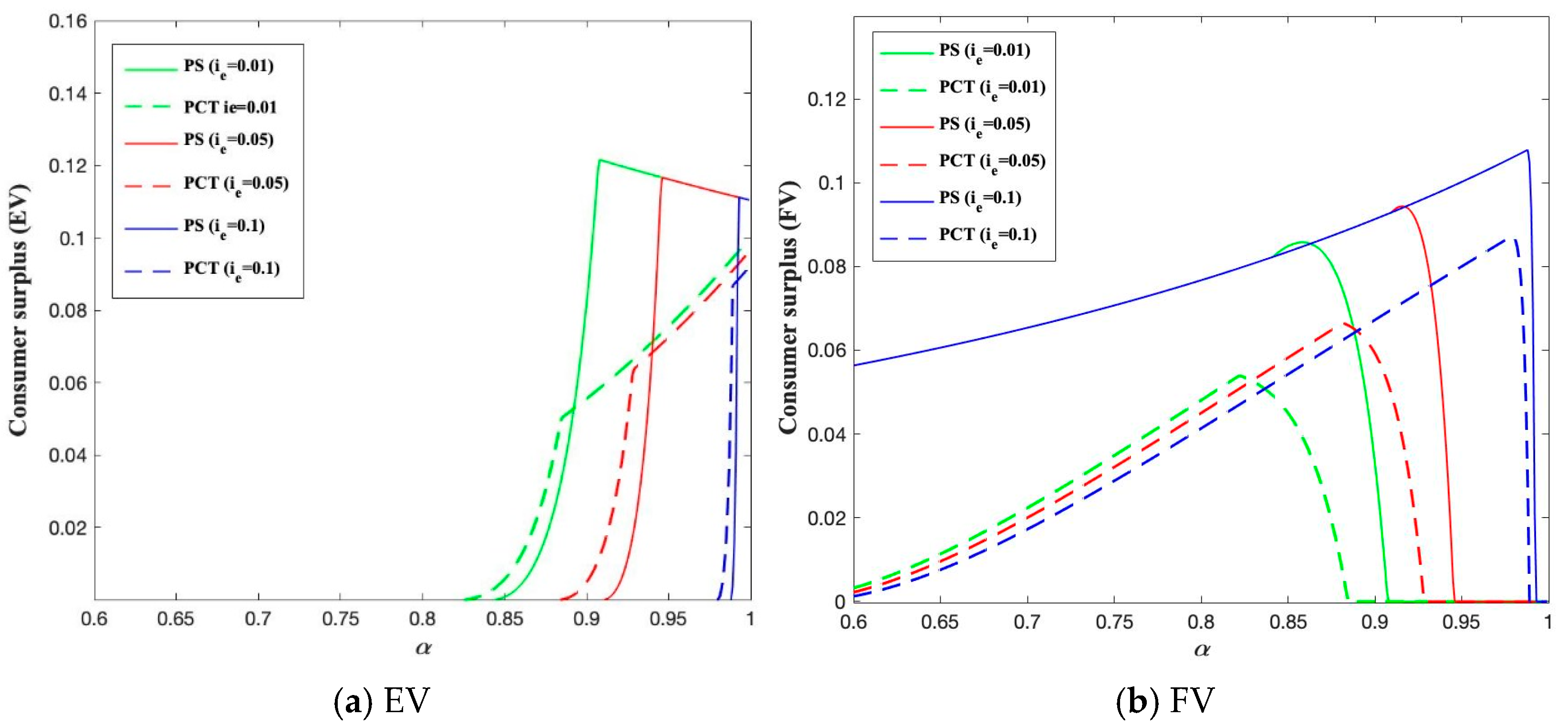
6.2. Comparison of PCT and PS When α < 1

In the scenario where α < 1 , we analyze the impact of changes in EV carbon emissions on different policies, including EV demand, FV demand, EV consumer surplus, FV consumer surplus, EV manufacturer’s profit, FV manufacturer’s profit, environmental benefits, and social welfare.
Figure 8 illustrates the impact of a difference in basic utility valuation on consumer surplus. Consistent with the results in Figure 4a, the consumer surplus for EVs under the PCT policy is greater than that under the PS policy when the coefficient of basic utility valuation difference is small. This can be attributed to the limited effectiveness of subsidies, which enhances the relative attractiveness of EVs under the PCT policy. Secondly, Figure 8b also indicates that the consumer surplus for FVs under the PS policy consistently exceeds that under the PCT policy, which indirectly validates the superiority of the PCT policy in promoting EV adoption from the perspective of consumers. Furthermore, the impact of EV carbon emissions on both EV consumer surplus and FV consumer surplus is similar. Specifically, as EV carbon emissions increase, the EV consumer surplus decreases while the FV consumer surplus increases. The above comparison and analysis of Figure 4 and Figure 8 can be summarized as the following Observation 1.
Observation 1. 
For FV consumer surplus, regardless of the difference in basic utility valuation, the consumer surplus under the PS policy always exceeds that under the PCT policy. However, for EV consumer surplus, when the difference in basic utility valuation is small, the consumer surplus under the PCT policy is higher than that under the PS policy, whereas the opposite is true when the difference in basic utility valuation is large.
Figure 9a,b describe the impact of the basic utility valuation difference on the demand of EVs and FVs. Under the PCT policy, the relationship between EV demand, as well as FV demand, and the basic utility valuation difference exhibits a similar pattern. Interestingly, under the PS policy, both EV demand and FV demand demonstrate a trend of initially increasing and then decreasing with the increase in the basic utility valuation difference. This contradicts the intuition that larger basic utility valuation differences would lead to a higher EV demand and a lower FV demand. The effect of EV carbon emissions on EV demand and FV demand is similar. Additionally, when α < 1 , the FV demand under the PS policy is also higher than under the PCT policy. This conclusion also confirms the inhibitory effect of the PCT policy on FV demand when α < 1 .
Figure 10a,b illustrate the variations in profits for EV manufacturers and FV manufacturers under different basic utility valuation differences. As depicted in Figure 10, it can be observed that under both policies, the profit of EV manufacturers exhibits a trend of initially increasing and then decreasing with the increase in the basic utility valuation difference, while decreasing with the increase in EV carbon emissions. Figure 10b reveals that under the PS policy, the profit of FV manufacturers decreases with the increase in the basic utility valuation difference, whereas under the PCT policy, the profit of FV manufacturers initially increases and then decreases with the increase in EV carbon emissions. Additionally, when the basic utility valuation difference is small, the profit of FV manufacturers decreases with the increase in EV carbon emissions, whereas when the basic utility valuation difference is large, the profit of FV manufacturers increases with the increase in EV carbon emissions. The above comparison and analysis of Figure 5, Figure 6, Figure 9 and Figure 10 can be summarized as the following Observation 2.
Observation 2. 
For FV demand and FV manufacturer profit, regardless of the level of the basic utility valuation difference, demand and profit under the PS policy will always be higher than under the PCT policy. For EV demand and EV manufacturer profit, when the basic utility valuation difference is small, the EV demand and profit of EV manufacturers under the PCT policy are higher than those under the PS policy, while the opposite is true when the basic utility valuation difference is large.
Figure 11a illustrates the variations in environmental benefits under different policies when α < 1 . Consistent with the scenario α > 1 , compared to the PS policy, government adoption of the PCT policy can effectively mitigate the negative environmental impacts of the transportation industry. Under the PS policy, as the basic utility valuation difference increases, the negative environmental impacts exhibit a trend of initially increasing and then decreasing, and with the increase in EV carbon emissions, the negative environmental impacts intensify. In the case of PCT, as the basic utility valuation difference increases, the negative environmental impacts also initially increase and then decrease. When the basic utility valuation difference is small, the increase in EV carbon emissions leads to a smaller negative environmental impact. Conversely, when the basic utility valuation difference is large, the increase in EV carbon emissions exacerbates the negative environmental impact.
Figure 11b illustrates the changes in social welfare under different policies. Consistent with Propositions 4 and 8, social welfare under both policies is influenced by the basic utility valuation difference and EV carbon emissions. As depicted in Figure 11b, holding other conditions constant, when the basic utility valuation difference is small, social welfare under the PS policy exceeds that under the PCT policy, whereas when the basic utility valuation difference is large, the PCT policy outperforms the PS policy. Regardless of whether it is the PCT or PS policy, as EV carbon emissions continue to increase, social welfare decreases. This finding echoes Proposition 2, suggesting that governments should integrate various efforts to enhance the environmental benefits of EVs and thus improve social welfare. As leaders in the game, governments should use their leadership roles to promote the enhancement of social welfare. The above comparison and analysis of Figure 7 and Figure 11 can be summarized as the following Observation 3.
Observation 3. 
For governments, the PCT policy consistently outperforms the PS policy in terms of environmental benefits. However, comparing the social welfare under the two policies, in the case of α > 1 , when the basic utility valuation difference is small, the overall social welfare of the PCT policy is higher than that of the PS policy. When the basic utility valuation difference is large, the overall social welfare of the PCT policy is lower than that of the PS policy. The situation where α < 1 is exactly the opposite.

7. Conclusions

Considering China’s effective promotion of the growing popularity of EVs through PS policy and, concurrently, the increasing adoption of PCT policy as regulatory tools in various international regions, it is particularly important and of profound significance to delve into the implementation effectiveness of these two policies across different application scenarios. The aim is to provide a scientific basis and strategic recommendations for the formulation and optimization of future related policies in our country. At present, some scholars have studied the application of PCT policy in promoting the development of the EV industry, but they have not considered the difference in basic utility valuation between EVs and FVs. By constructing a three-stage game model composed of government, manufacturers, and consumers, this paper examines the optimal decision of PCT policy and PS policy under the condition of basic utility valuation heterogeneity. Through the analysis, this paper obtains the following findings.

7.1. Findings

Firstly, under certain conditions, blindly increasing subsidies or raising carbon taxes may not effectively improve social welfare and could even have negative consequences. It is closely related to the valuation differences among consumers in the region. This is because the government’s determination of optimal subsidies and carbon taxes is influenced by various factors, such as EV carbon emissions, FV carbon emissions, and consumers’ low-carbon preferences. Our results also emphasize the critical role of basic utility valuation in determining differences in social welfare. Specifically, in regions with rapid EV industry development (e.g., China, Norway), as consumer preference for EVs increases, social welfare under the PCT policy initially surpasses that under the PS policy. However, as preferences continue to expand, social welfare under the PS policy exceeds that under the PCT policy. Interestingly, the opposite occurs in regions with slower EV industry development (e.g., Japan, Germany). From an environmental benefits perspective, the PCT (personal carbon tax) policy is always superior to the PS (purchase subsidy) policy. This finding can effectively assist the government in achieving the goal of reducing the negative environmental impact of the transportation sector through PCT policies.
Secondly, this research demonstrates that the government exhibits a preference in formulating policies for promoting the EV market. When the environmental benefits of EVs are significant, the government is more inclined to adopt proactive policy measures, such as providing more substantial subsidies or imposing higher carbon taxes. This is because significant environmental benefits imply that implementing economic incentives at this time can maximize the impact of the policies. When the environmental benefits of EVs are not evident, the government’s policy stance tends to be more conservative, such as offering fewer subsidies or setting lower carbon taxes. This conservative approach helps avoid excessive waste of fiscal resources and reduces the industry’s overreliance on governmental financial incentives. In summary, this preference for policies that consider the level of EV environmental benefits highlights the critical role of EV environmental performance in government decision-making.
Thirdly, consumer surplus for EVs under the PS policy does not always surpass that under the PCT policy. The study finds that when the difference in basic utility valuation is small, consumer surplus for EVs under the PCT policy is higher. This is because although the subsidies under the PS policy can increase consumer surplus, this increase effect is limited and depends on the amount of subsidy. In other words, when the difference in basic utility valuation is small and the difference between the two types of vehicles is small, even without subsidies under the PCT policy, consumers tend to choose EVs to avoid paying additional carbon taxes. In such cases, the PCT policy enhances the relative attractiveness of EVs, resulting in higher consumer surplus for purchasing EVs under this policy than under the PS policy. Interestingly, our findings also confirm another common perception, namely, that consumer surplus for FVs under the PS policy always exceeds that under the PCT policy. This is because the carbon tax increases the purchase cost of FVs, thereby reducing consumer surplus. Under the PS policy, as no measures are taken against FV consumers, the price of FVs remains unchanged, thus consumer surplus remains unaffected directly.
Finally, surprisingly, for manufacturers, both scenarios where the basic utility valuation difference coefficient is greater than 1 and less than 1 exhibit similar trends. With the increase in the difference in basic utility valuation, initially, the demand for EVs and the profits for EV manufacturers under the PCT policy are higher than under the PS policy. However, with further increases in the valuation difference, the demand for EVs and the profits for EV manufacturers under the PS policy exceed those under the PCT policy. Through this analysis, it is evident that neither the PS policy nor the PCT policy is a one-size-fits-all approach for expanding the EV market demand, and manufacturing enterprises need to make policy choices based on specific market conditions. However, the situation for FVs is quite different. This finding not only reveals the inhibitory effect of the PCT policy on traditional FVs but also confirms the positive role of this policy in accelerating the transformation of traditional automotive companies and updating industrial structures.

7.2. Practical Contributions

This study provides the following insights into industrial practice. Firstly, at the government policy level, it is recommended to establish a policy adaptation mechanism based on regional valuation differences. Specifically, this involves quantifying the regional basic utility valuation disparity coefficient and dividing the national market into three categories: high, medium, and low utility valuation disparity zones. In terms of policy implementation, regional economic characteristics and consumer preference structures should be fully considered in countries with rapid EV industry development, such as China and the United States. The rise of local companies like BYD and Tesla has strengthened consumer preference for EVs. These regions can be categorized as high valuation difference areas, where PS policies are suitable to enhance consumption incentives. In contrast, for some Middle Eastern countries with slower EV industry growth, consumer acceptance of EVs is limited due to cultural traditions and resource constraints. These areas can be categorized as low valuation difference areas, where implementing PCT policies through price mechanisms to guide industrial transformation may result in better social welfare outcomes. Therefore, it is recommended to establish a dynamic regional policy evaluation framework, adjusting regional classification standards based on market monitoring data, and implementing differentiated policy mechanisms to maximize policy effectiveness.
Finally, for manufacturing enterprises, relying solely on policy funding support to increase the market demand for EVs is not conducive to the long-term development of their own businesses and the whole industry. Instead, enterprises should start with the research and development of EV performance itself to enhance the perceived utility valuation of cars to consumers. Furthermore, genuine long-term expansion of the EV market can only be achieved through resource integration with the government to promote technological innovation and improvement. For consumers, actively acquiring relevant information and understanding the impact of different policies on the environment and social welfare are crucial. Consumers should make more rational and responsible purchase decisions based on their actual needs, thereby driving policies towards directions that align with the interests of the majority. In this process, consumer behavior not only represents individual choices but also influences and shapes the entire industry environment.

7.3. Future Research Directions

The three-stage Stackelberg game model constructed in this study effectively simulates the decision-making interactions between consumers, manufacturers, and the government. However, there are several limitations. First, in terms of model construction, the study focuses on the core relationship between the coefficient of consumer utility valuation differences and policy tool selection but does not fully incorporate spatial heterogeneity factors (such as regional differences in charging infrastructure coverage), the diversity of corporate competition strategies (such as the coexistence of price alliances and differentiated competition), and the complexity of the supply chain market (with diverse production and sales forms). Second, in terms of research content, the study simplifies consumers into two groups based on preferences for EVs and FVs, exploring their preferences for PS and PCT policies, without sufficiently considering consumer diversity and the synergistic effects of the two policies. Finally, in terms of research conclusions, although the study reveals the moderating role of carbon emission levels in optimal policy formulation, it does not establish a framework for determining the boundary conditions of policy applicability.
This paper proposes three directions for future research in this field. First, incorporating spatial heterogeneity parameters (such as regional infrastructure disparities) and the manufacturer’s competition game mechanism (such as price alliances or differentiation strategies) to make the model more aligned with industry realities. Second, based on consumer segmentation theory, constructing a heterogeneous utility function that includes multiple dimensions, such as technological preferences, environmental awareness, and price sensitivity. Third, exploring the moderating effects of other key variables on optimal policy formulation, such as consumer low-carbon preference coefficients and cost difference coefficients, to further analyze the boundary conditions for policy applicability.

Author Contributions

Data curation, J.Z.; formal analysis, P.L.; funding acquisition, L.C.; investigation, L.S., J.Z., P.L. and Z.Z.; methodology, L.S. and P.L.; resources, L.S.; software, J.Z.; supervision, Z.Z. and L.C.; writing—original draft, L.S., J.Z., P.L., Z.Z. and L.C.; writing—review and editing, L.S., J.Z., P.L., Z.Z. and L.C. All authors have read and agreed to the published version of the manuscript.

Funding

This research was supported by a research grant from the National Natural Science Foundation of China (No. 72102171), the Humanities and Social Sciences Youth Foundation, Ministry of Education of the People’s Republic of China (No. 21YJC630006), the Hubei Provincial Social Science Foundation, General Project (No. HBSKJJ20243252), and the Graduate Education Innovation Fund of Wuhan Institute of Technology (No. CX2024133).

Data Availability Statement

The original contributions presented in this study are included in the article. Further inquiries can be directed to the corresponding authors.

Conflicts of Interest

The authors declare no conflicts of interest.

Appendix A

Proof for Solving the Optimal Decision

(1) 
PS ( α > 1 )
According to consumers’ purchase behavior, the manufacturers determine the retail prices for EV and FV based on the principle of maximizing their own interests. Let π e p e = 0 and π g p g = 0 to obtain the retail prices for EV and FV. Substituting these prices into Equation (5), we can derive the optimal market demand for EVs and FVs, as shown in Equation (6).
To ensure the practical effectiveness of this study, it is necessary to have 2 α 1 i e β α i g β + 2 α k α k c 2 α α 1 2 α 1 = R m i n < R < R m a x = α α 1 + α i e β + α 2 α 2 i g β + α k + α 2 α 2 c α in this case, to guarantee that the market demand for EVs and FVs in Equation (6) is non-negative. Under this condition, the requirement θ 2 < θ 1 < 1 is met. Furthermore, in order to ensure R m i n R m a x , it is also required that c 1 β i g .
Substituting Equation (6) into Equation (4) yields the undifferentiated points θ 1 and θ 2 , as shown in Equation (7). Through the above calculations, the social welfare function can be obtained as shown in the following:
θ 1 p s + = 2 α 1 i e β α i g β + 2 α k α k c + 1 2 α R + 2 α 1 α 1 4 α 1 α 1
θ 2 p s + = i e β + 2 α i g β + 2 α + k c R + α 1 4 α 1
(2) 
PS ( α < 1 )
Similar to the case when α > 1 , the manufacturers make decisions to maximize their own interests. By setting π e p e = 0 and π g p g = 0 , we can obtain the optimal retail price and the market demands for EVs and FVs, as shown in Equation (10).
2 α i e β α i g β α k + α 2 k c + α α 1 2 α = R m i n < R < R m a x = 2 1 α + i e β 2 α i g β 2 α k c to ensure that the market demands for EVs and FVs are non-negative. Under this condition, it is ensured that θ 2 < θ 1 < 1 . Furthermore, to guarantee that R m i n R m a x , 1 β i g c 0 must also be satisfied.
Using the same method in Section 4.1, we can obtain the social welfare function and the undifferentiated points θ 1 and θ 2 , when α < 1 under the PS policy, as shown in the following:
θ 1 p s = i e β + 2 α i g β + 2 α k c + R + 2 α 1 α 4 α 1 α
θ 2 p s = 2 i e β + α i g β + 2 k + α c 2 R + α α 2 4 α α
(3) 
PCT ( α > 1 )
Setting π e p e = 0 and π g p g = 0 yields the optimal retail prices for EVs and FVs. By substituting this into Equation (12), the optimal market demands for EVs and FVs are obtained, as shown in Equation (13).
2 α α 1 + 2 α 1 β i e α β i g + 2 α k α k c α = T m i n T T m a x = α α 1 + α β i e + α 1 2 α β i g + α k + 1 2 α c α 2 α 1 to ensure that the market demands for EVs and FVs are non-negative. Under this condition, it is ensured that θ 2 < θ 1 < 1 . Furthermore, to guarantee that T m i n T m a x , α β i e c k 0 must also be satisfied.
Substituting Equation (13) into Equation (12) yields the undifferentiated points θ 1 and θ 2 , as shown in Equation (14). Similar to the method of calculating the social welfare function under the PS policy, the social welfare function can be derived as shown in Equation (14). It is worth noting that government revenue refers to the total amount of taxes levied on consumers who purchase FVs.
θ 1 p c t + = 2 α 1 β i e α β i g + 2 α k α k c α i g i e T + 2 α 1 α 1 4 α 1 α 1
θ 2 p c t + = β i e + 2 α β i g + 2 α + k c + 2 α i g i e T + α 1 4 α 1
(4) 
PCT ( α < 1 )
Setting π e p e = 0 and π g p g = 0 yields the optimal retail prices for EV and FV. Substituting into Equation (15), we obtain the optimal market demands for EV and FV, as presented in Equation (13).
α 1 α + 2 α β i e α β i g α k + α 2 k c α = T m i n < T < T m a x < 2 2 α + β i e + α 2 β i g 2 α k c 2 α to ensure that the market demands for EVs and FVs are non-negative. Under this condition, it is ensured that θ 2 < θ 1 < 1 . Furthermore, to guarantee that T m i n T m a x , α β i e c k 0 must also be satisfied.
Using the same method in Section 4.1, we can obtain the social welfare function and the undifferentiated points θ 1 and θ 2 , when α < 1 under the PCT policy, as shown in the following:
θ 1 p c t = β i e + 2 α β i g + 2 α k c + 2 α i g i e T + 2 3 α + α 2 4 α 1 α
θ 2 p c t = 2 β i e + α β i g + α + 2 k c + α i g i e T + α α 2 4 α α
Proof of Lemma 1. 
q e p s + α = 2 + 4 α 2 α 2 + c 4 α 2 c + 3 c k 8 α c k + 8 α 2 c k 3 R + 8 α R 8 α 2 R + 3 8 α + 8 α 2 β i e + β 4 α 2 β i g 1 4 α 2 1 + α 2 , when R 1 = 2 + 4 α 2 α 2 + c 4 α 2 c + 3 c k 8 α c k + 8 α 2 c k + 3 β i e 8 α β i e + 8 α 2 β i e + β i g 4 α 2 β i g 3 8 α + 8 α 2 , q e p s + α = 0 . R 1 R m i n = 1 5 α + 4 α 2 2 4 α + 4 α 2 c β i g 1 + 2 α 3 8 α + 8 α 2 > 0 , R m a x R 1 = 1 + 7 α 14 α 2 + 8 α 3 1 + 2 c + 2 β i g 3 8 α + 8 α 2 . When 1 2 β i g 2 < c < 1 β i g , R 1 > R m a x , at this time the value of each R is guaranteed q e p s + α > 0 , q e p s + increases with the increase in α . When 0 < c < 1 2 β i g 2 , R m i n < R 1 < R m a x . When R m i n < R < R 1 , q e p s + α > 0 , q e p s + increases with the increase in α . When R 1 < R < R m a x , q e p s + α < 0 , q e p s + decreases with the increase in α .
q g p s + α = 1 + 2 α α 2 + c 4 α c + 6 α 2 c + c k 4 α 2 c k R + 4 α 2 R + β 4 α 2 β i e + 1 4 α + 6 α 2 β i g 1 4 α 2 1 + α 2 , when R 2 = 1 2 α + α 2 c + 4 α c 6 α 2 c c k + 4 α 2 c k β i e + 4 α 2 β i e β i g + 4 α β i g 6 α 2 β i g 1 + 4 α 2 , q g p s + α = 0 . R 2 R m i n = 1 5 α + 4 α 2 1 + α c β i g 1 + 4 α 2 > 0 , R m a x R 1 = α 1 5 α + 4 α 2 1 + 2 c + 2 β i g 1 + 4 α 2 . When 1 2 β i g 2 < c < 1 β i g , R 2 > R m a x , at this time the value of each R is guaranteed q g p s + α > 0 , q g p s + increases with the increase in α . When 0 < c < 1 2 β i g 2 , R m i n < R 2 < R m a x . When R m i n < R < R 2 , q g p s + α > 0 , q g p s + increases with the increase in α . When R 2 < R < R m a x , q g p s + α < 0 , q g p s + decreases with the increase in α . □
Proof of Lemma 2. 
q e p c t + α = 2 1 + α 2 + 3 + 8 1 + α α β i e + β 4 α 2 β i g + c 1 4 α 2 + 3 k + 8 1 + α α k + 1 4 α 2 T 1 5 α + 4 α 2 2 , when T 1 = 3 8 α + 8 α 2 β i e 4 α 2 1 β i g 2 α 1 2 + c 1 4 α 2 + 3 8 α + 8 α 2 k 4 α 2 1 , q e p c t + α = 0 . T 1 T m i n = 1 5 α + 4 α 2 2 α 2 c k β i e α 1 + 4 α 2 > 0 , T m a x T 1 = 1 5 α + 4 α 2 1 + 2 c k + 2 β i e 1 + 4 α 2 . When 1 2 β i e 2 k < c < a β i e k , T 1 > T m a x , at this time the value of each T is guaranteed q e p c t + α > 0 , q e p c t + increases with the increase in α . When 0 < c < 1 2 β i e 2 k , T m i n < T 1 < T m a x . When T m i n < T < T 1 , q e p c t + α > 0 , q e p c t + increases with the increase in α . When T 1 < T < T m a x , q e p c t + α < 0 , q e p c t + decreases with the increase in α .
q g p c t + α = 2 1 + α 2 + 3 + 8 1 + α α β i e + β 4 α 2 β i g + c 1 4 α 2 + 3 k + 8 1 + α α k + 1 4 α 2 T 1 5 α + 4 α 2 2 , when T 2 = 1 + α 2 + β 4 α 2 β i e + 1 4 α + 6 α 2 β i g + c 1 4 α + α 2 6 4 k + k + 1 4 α + 6 α 2 T 1 5 α + 4 α 2 2 , q g p c t + α = 0 . T 2 T m i n = 1 5 α + 4 α 2 3 α 2 + c k α 1 + 2 c k + β 2 α β i e α 1 4 α + 6 α 2 > 0 , T m a x T 2 = α 1 5 α + 4 α 2 1 + 2 c k + 2 β i e 1 + 2 α 1 4 α + 6 α 2 . When 1 2 β i e 2 k < c < α β i e k , T 2 > T m a x , at this time the value of each T is guaranteed q g p c t + α > 0 , q g p c t + increases with the increase in α . When 0 < c < 1 2 β i e 2 k , T m i n < T 2 < T m a x . When T m i n < T < T 2 , q g p c t + α > 0 , q g p c t + increases with the increase in α . When T 1 < T < T m a x , q g p c t + α < 0 , q g p c t + decreases with the increase in α . □
Proof of Propositions 1 and 2. 
When S W p s + R = 0 , in this case R ^ = 3 α 7 α 2 + 4 α 3 2 α c + 4 α 2 c c k + 3 α c k 4 α 2 c k + 3 α R 4 α 2 R 1 + β 3 α 2 + β + 4 α 2 2 + β i e + α 1 2 β + 4 α 1 + β i g 1 4 α 2 1 + α , which means that when R = R ^ , the overall social welfare is maximized. At the same time, to ensure that the demand is positive, R needs to satisfy R m i n R R m a x . When R m a x = R ^ , i e 2 = α c + 2 α 2 c + c k 2 α c k + a i g a β i g + 2 α 2 β i g 1 + 2 α 1 + β . So when i e i e 2 , R m a x R ^ , the maximum point R ^ is on the right side of the value range. When R [ R m i n , R m a x ] , S W p s + R > 0 , the overall social welfare increases with the increase in R . When R m i n = R ^ , i e 1 = 3 α 7 α 2 + 4 α 3 2 α c + 3 α 2 c c k + 4 α c k 4 α 2 c k α i g + 2 α 2 i g 2 α β i g + 3 α 2 β i g 1 + 2 α 2 1 + β . So when i e i e 1 , R m i n R ^ , the maximum point R ^ is on the left side of the value range. When R [ R m i n , R m a x ] , S W p s + R < 0 , the overall social welfare decreases with the increase in R . When i e 2 < i e < i e 1 , R m i n < R ^ < R m a x , if R [ R m i n , R ^ ] , then S W p s + R > 0 , that is, the overall social welfare increases with the increase in R ; If R R ^ , R m a x , then S W p s + R < 0 , that is, the overall social welfare decreases with the increase in R . In summary, when i e i e 2 , if R = R m a x , then the overall social welfare is the largest. When i e 1 i e , if R = R m i n , then the overall social welfare is the largest. When i e 2 < i e < i e 1 , if R = R ^ , then the social welfare is the largest. □
Proof of Propositions 3 and 4. 
The proofs of Propositions 3 and 4 are similar to those of Propositions 1 and 2. □
Proof of Propositions 5 and 6. 
When S W p c t + T = 0 , in this case T ^ = α 1 + i e 1 + 2 β 4 α 4 α β + i g 1 + β + i g 4 α 3 2 + β α + 1 + 2 k + α 4 α 3 4 k c α 4 α 3 . To ensure that the demand is positive, T needs to satisfy T m i n T T m a x . When T m a x = T ^ , i e 1 = 2 α 1 α 1 + 2 α 1 β + 1 i g c 2 α 1 k 1 2 α 1 β + 1 . So when i e i e 1 , T m a x T ^ , the maximum point T ^ is on the right side of the value range. When T [ T m i n , T m a x ] , S W p c t + T > 0 , the overall social welfare increases with the increase in T . When T m i n = T ^ , i e 2 = ( α 1 ) 2 + 1 + β ( 2 α 1 ) 2 i g + c 1 + 2 k 4 α 3 α k + 4 α 2 α 2 + 3 β 2 β + 1 . Therefore, when i e i e 2 , T m i n T ^ , the maximum point T ^ is on the left side of the value range. When T [ T m i n , T m a x ] , S W p c t + T < 0 , the overall social welfare decreases with the increase in T . When i e 1 < i e < i e 2 , T m i n < T ^ < T m a x , if T [ T m i n , T ^ ] , then S W p c t + T > 0 , that is, the overall social welfare increases with the increase in T ; If T T ^ , T m a x , then S W p c t + T < 0 , that is, the overall social welfare decreases with the increase in T . In summary, when i e i e 1 , if T = T m a x , then the overall social welfare is the largest. When i e 2 i e , if T = T m i n , then the overall social welfare is the largest. When i e 1 < i e < i e 2 , if T = T ^ , then the overall social welfare is the largest. □
Proof of Propositions 7 and 8. 
The proofs of Propositions 7 and 8 are similar to those of Propositions 5 and 6. □

References

  1. Anufriev, I.E.; Khusainov, B.; Tick, A.; Devezas, T.; Sarygulov, A.; Kaimoldina, S. Mathematical model for assessing new, non-fossil fuel technological products (li-Ion batteries and electric vehicle). Mathematics 2025, 13, 143. [Google Scholar] [CrossRef]
  2. Chen, L.; Dong, T.; Li, X.; Xu, X. Logistics engineering management in the platform supply chain: An overview from logistics service strategy selection perspective. Engineering 2025, 47, 236–249. [Google Scholar] [CrossRef]
  3. Fang, L.; Li, Y.; Govindan, K. Entry mode selection for a new entrant of the electric vehicle automaker. Eur. J. Oper. Res. 2024, 313, 270–280. [Google Scholar] [CrossRef]
  4. Ma, H.; Yang, R.; Li, X. Delivery routing for a mixed fleet of conventional and electric vehicles with road restrictions. Int. J. Prod. Res. 2024, 1–24. [Google Scholar] [CrossRef]
  5. Zhang, W.; Dou, Y. Coping with spatial mismatch: Subsidy design for electric vehicle and charging markets. Manuf. Serv. Oper. Manag. 2022, 24, 1595–1610. [Google Scholar] [CrossRef]
  6. Abouee-Mehrizi, H.; Baron, O.; Berman, O.; Chen, D. Adoption of electric vehicles in car sharing market. Prod. Oper. Manag. 2021, 30, 190–209. [Google Scholar] [CrossRef]
  7. Qiu, Y.; Ding, S.; Pardalos, P.M. Routing a mixed fleet of electric and conventional vehicles under regulations of carbon emissions. Int. J. Prod. Res. 2024, 62, 5720–5736. [Google Scholar] [CrossRef]
  8. Liu, J.; Li, L.; He, L.; Ma, X.; Yuan, H. Consumers or infrastructure firms? Who should the government subsidize to promote electric vehicle adoption when considering the indirect network and herd effects. Transp. Policy 2024, 149, 163–176. [Google Scholar] [CrossRef]
  9. Song, Y.; Li, G.; Wang, Q.; Meng, X.; Wang, H. Scenario analysis on subsidy policies for the uptake of electric vehicles industry in China. Resour. Conserv. Recycl. 2020, 161, 104927. [Google Scholar] [CrossRef]
  10. He, C.; Ozturk, O.C.; Gu, C.; Chintagunta, P.K. Consumer tax credits for EVs: Some quasi-experimental evidence on consumer demand, product substitution, and carbon emissions. Manag. Sci. 2023, 69, 7759–7783. [Google Scholar] [CrossRef]
  11. Chung, H.; Ahn, H.S.; Lee, M.; Kim, S.W. Optimal subsidy policy for innovation: Technology push and demand pull. Prod. Oper. Manag. 2024, 33, 817–831. [Google Scholar] [CrossRef]
  12. Wang, C.; Sun, H.; Wang, Y. Synergy and effectiveness evaluation of carbon policy and government subsidies: Variational inequality model based on supply chain network. Mathematics 2025, 13, 1099. [Google Scholar] [CrossRef]
  13. Yang, S.; Cheng, P.; Li, J.; Wang, S. Which group should policies target? Effects of incentive policies and product cognitions for electric vehicle adoption among Chinese consumers. Energy Policy 2019, 135, 111009. [Google Scholar] [CrossRef]
  14. Xia, L.; Gao, S.; Wei, J.; Ding, Q. Government subsidy and corporate green innovation-Does board governance play a role? Energy Policy 2022, 161, 112720. [Google Scholar] [CrossRef]
  15. Harvey, L.D. Rethinking electric vehicle subsidies, rediscovering energy efficiency. Energy Policy 2020, 146, 111760. [Google Scholar] [CrossRef]
  16. Mohammadzadeh, N.; Zegordi, S.H.; Kashan, A.H.; Nikbakhsh, E. Optimal government policy-making for the electric vehicle adoption using the total cost of ownership under the budget constraint. Sustain. Prod. Consum. 2022, 33, 477–507. [Google Scholar] [CrossRef]
  17. Li, K.; Wang, L. Optimal electric vehicle subsidy and pricing decisions with consideration of EV anxiety and EV preference in green and non-green consumers. Transp. Res. Part E Logist. Transp. Rev. 2023, 170, 103010. [Google Scholar] [CrossRef]
  18. Huang, C.Y.; Chen, Z.; Fan, Z.P.; Zhang, Q. Sharing mode selection and optimal pricing for an electric vehicle manufacturer. Int. J. Gen. Syst. 2024, 53, 403–425. [Google Scholar] [CrossRef]
  19. Shi, L.; Sethi, S.P.; Çakanyıldırım, M. Promoting electric vehicles: Reducing charging inconvenience and price via station and consumer subsidies. Prod. Oper. Manag. 2022, 31, 4333–4350. [Google Scholar] [CrossRef]
  20. Li, W.; Long, R.; Chen, H.; Yang, M.; Chen, F.; Zheng, X.; Li, C. Would personal carbon trading enhance individual adopting intention of battery electric vehicles more effectively than a carbon tax? Resour. Conserv. Recycl. 2019, 149, 638–645. [Google Scholar] [CrossRef]
  21. Mohammadzadeh, N.; Zegordi, S.H.; Nikbakhsh, E. Pricing and free periodic maintenance service decisions for an electric-and-fuel automotive supply chain using the total cost of ownership. Appl. Energy 2021, 288, 116471. [Google Scholar] [CrossRef]
  22. Srivastava, A.; Kumar, R.R.; Chakraborty, A.; Mateen, A.; Narayanamurthy, G. Design and selection of government policies for electric vehicles adoption: A global perspective. Transp. Res. Part E Logist. Transp. Rev. 2022, 161, 102726. [Google Scholar] [CrossRef]
  23. Fawcett, T. Personal carbon trading: A policy ahead of its time? Energy Policy 2010, 38, 6868–6876. [Google Scholar] [CrossRef]
  24. Xie, F.; Liu, N.; Jin, M.; Lin, Z. Impacts of the consumer heterogeneity in fuel economy valuation on compliance with fuel economy standards. Energy 2019, 177, 167–174. [Google Scholar] [CrossRef]
  25. He, H.; Wang, C.; Wang, S.; Ma, F.; Sun, Q.; Zhao, X. Does environmental concern promote EV sales? Duopoly pricing analysis considering consumer heterogeneity. Transp. Res. Part D Transp. Environ. 2021, 91, 102695. [Google Scholar] [CrossRef]
  26. Behnood, A.; Haghani, M.; Golafshani, E.M. Determinants of purchase likelihood for partially and fully automated vehicles: Insights from mixed logit model with heterogeneity in means and variances. Transp. Res. Part A Policy Pract. 2022, 159, 119–139. [Google Scholar] [CrossRef]
  27. Jia, W.; Chen, T.D. Investigating heterogeneous preferences for plug-in electric vehicles: Policy implications from different choice models. Transp. Res. Part A Policy Pract. 2023, 173, 103693. [Google Scholar] [CrossRef]
  28. Cheng, Y.; Fan, T. Production coopetition strategies for an FV automaker and a competitive NEV automaker under the dual-credit Policy. Omega 2021, 103, 102391. [Google Scholar] [CrossRef]
  29. Yi, Y.; Zhang, M.; Zhang, A.; Li, Y. Can “dual credit” replace “subsidies” successfully?-based on analysis of vehicle supply chain decisions under the digital transformation of technology. Energy Econ. 2024, 130, 107303. [Google Scholar] [CrossRef]
  30. Nie, Q.; Zhang, L.; Li, S. How can personal carbon trading be applied in electric vehicle subsidies? A Stackelberg game method in private vehicles. Appl. Energy 2022, 313, 118855. [Google Scholar] [CrossRef]
  31. Wang, N.; Shang, K.; Liu, H.; Duan, Y.; Qin, D. How carbon trading policy should be integrated with existing industrial policies: A case study of Chinese automotive industry. Appl. Energy 2025, 384, 125442. [Google Scholar] [CrossRef]
  32. Yu, Y.; Zha, D.; Zhou, D.; Wang, Q. Promoting the adoption of electric vehicles through private charging infrastructure: Should subsidies be for the builder or non-builder? Transp. Res. Part A Policy Pract. 2025, 192, 104368. [Google Scholar] [CrossRef]
  33. Chen, T.; Zheng, X.X.; Jia, F.; Koh, L. Toward mass adoption of electric vehicles: Policy optimisation under different infrastructure investment scenarios. Int. J. Prod. Res. 2025, 1–26. [Google Scholar] [CrossRef]
  34. Shao, L.; Yang, J.; Zhang, M. Subsidy scheme or price discount scheme? Mass adoption of electric vehicles under different market structures. Eur. J. Oper. Res. 2017, 262, 1181–1195. [Google Scholar] [CrossRef]
  35. Kumar, R.R.; Chakraborty, A.; Mandal, P. Promoting electric vehicle adoption: Who should invest in charging infrastructure? Transp. Res. Part E Logist. Transp. Rev. 2021, 149, 102295. [Google Scholar] [CrossRef]
  36. Liao, H.; Peng, S.; Li, L.; Zhu, Y. The role of governmental policy in game between traditional fuel and new energy vehicles. Comput. Ind. Eng. 2022, 169, 108292. [Google Scholar] [CrossRef]
  37. Fan, Z.P.; Cao, Y.; Huang, C.Y.; Li, Y. Pricing strategies of domestic and imported electric vehicle manufacturers and the design of government subsidy and tariff policies. Transp. Res. Part E Logist. Transp. Rev. 2020, 143, 102093. [Google Scholar] [CrossRef]
  38. Zhang, J.; Huang, J. Vehicle product-line strategy under government subsidy programs for electric/hybrid vehicles. Transp. Res. Part E Logist. Transp. Rev. 2021, 146, 102221. [Google Scholar] [CrossRef]
  39. Xu, Y.; Tian, Y.; Pang, C.; Tang, H. Manufacturer vs. Retailer: A comparative analysis of different government subsidy strategies in a dual-channel supply chain considering green quality and channel preferences. Mathematics 2024, 12, 1433. [Google Scholar] [CrossRef]
  40. Ashraf, F.; Equbal, A.; Khan, O.; Yahya, Z.; Alhodaib, A.; Parvez, M.; Ahmad, S. Assessment and ranking of different vehicles carbon footprint: A comparative study utilizing entropy and TOPSIS methodologies. Green Technol. Sustain. 2025, 3, 100128. [Google Scholar] [CrossRef]
  41. Yu, Y.; Zhou, D.; Zha, D.; Wang, Q.; Zhu, Q. Optimal production and pricing strategies in auto supply chain when dual credit policy is substituted for subsidy policy. Energy 2021, 226, 120369. [Google Scholar] [CrossRef]
  42. Liu, J.; Zhao, H.; Li, J.; Yue, X. Operational strategy of customized bus considering customers’ variety seeking behavior and service level. Int. J. Prod. Econ. 2021, 231, 107856. [Google Scholar] [CrossRef]
  43. Zhang, Q.; Liu, Y. Promoting electric vehicle adoption in ride-hailing platforms: To control or subsidize? Comput. Ind. Eng. 2024, 191, 110146. [Google Scholar] [CrossRef]
  44. Wang, Z.; Li, X. Demand subsidy versus production regulation: Development of new energy vehicles in a competitive environment. Mathematics 2021, 9, 1280. [Google Scholar] [CrossRef]
  45. Yang, A.; Liu, C.; Yang, D.; Lu, C. Electric vehicle adoption in a mature market: A case study of Norway. J. Transp. Geogr. 2023, 106, 103489. [Google Scholar] [CrossRef]
  46. Li, C.; Lu, X.; Liu, Y.; Xia, Z.; Wang, X.; Zhao, H. A study of tripartite strategies for closed-loop charging infrastructure construction of new energy vehicles in China under the expectation of government withdrawal subsidies. J. Clean. Prod. 2025, 493, 144943. [Google Scholar] [CrossRef]
  47. Deng, R.; Shen, N.; Zhao, Y. Diffusion model to analyse the performance of electric vehicle policies: An evolutionary game simulation. Transp. Res. Part D Transp. Environ. 2024, 127, 104037. [Google Scholar] [CrossRef]
  48. Bao, B.; Ma, J.; Goh, M. Short-and long-term repeated game behaviours of two parallel supply chains based on government subsidy in the vehicle market. Int. J. Prod. Res. 2020, 58, 7507–7530. [Google Scholar] [CrossRef]
  49. Han, Z.; Si, Y.; Wang, X.; Yang, S. Battery mode selection and carbon emission decisions of competitive electric vehicle manufacturers. Mathematics 2024, 12, 2472. [Google Scholar] [CrossRef]
  50. Varian, H.R. Microeconomic Analysis; W. W. Norton & Company: New York, NY, USA, 1992. [Google Scholar]
  51. Bian, J.; Zhang, G.; Zhou, G. Manufacturer vs. consumer subsidy with green technology investment and environmental concern. Eur. J. Oper. Res. 2020, 287, 832–843. [Google Scholar] [CrossRef]
  52. Liu, C.; Huang, W.; Yang, C. The evolutionary dynamics of China’s electric vehicle industry–Taxes vs. subsidies. Comput. Ind. Eng. 2017, 113, 103–122. [Google Scholar] [CrossRef]
  53. Okada, T.; Tamaki, T.; Managi, S. Effect of environmental awareness on purchase intention and satisfaction pertaining to electric vehicles in Japan. Transp. Res. Part D Transp. Environ. 2019, 67, 503–513. [Google Scholar] [CrossRef]
  54. Bunsen, T.; Cazzola, P.; Gorner, M.; Paoli, L.; Scheffer, S.; Schuitmaker, R.; Teter, J. Global EV Outlook 2018: Towards Cross-Modal Electrification; International Energy Agency: Paris, France, 2018. [Google Scholar]
  55. Cen, X.; Lo, H.K.; Li, L. A framework for estimating traffic emissions: The development of passenger car emission unit. Transp. Res. Part D Transp. Environ. 2016, 44, 78–92. [Google Scholar] [CrossRef]
  56. Crane, K.; Mao, Z. Costs of Selected Policies to Address Air Pollution in China; RAND Corporation: Santa Monica, CA, USA, 2015. [Google Scholar]
Figure 1. The decision-making process among the three participants.
Systems 13 00506 g001
Figure 2. Different behaviors of the heterogeneous consumers when α > 1 .
Systems 13 00506 g002
Figure 3. Different behaviors of the heterogeneous consumers when α < 1 .
Systems 13 00506 g003
Figure 4. Consumer surplus ( α > 1 ) .
Systems 13 00506 g004
Figure 5. Market demand ( α > 1 ) .
Systems 13 00506 g005
Figure 6. Manufacturers’ profits ( α > 1 ) .
Systems 13 00506 g006
Figure 7. Governmental analysis perspective ( α > 1 ) .
Systems 13 00506 g007
Figure 8. Consumer surplus ( α < 1 ) .
Systems 13 00506 g008
Figure 9. Market demand ( α < 1 ) .
Systems 13 00506 g009
Figure 10. Manufacturers’ profits ( α < 1 ) .
Systems 13 00506 g010
Figure 11. Governmental analysis perspective ( α < 1 ) .
Systems 13 00506 g011
Table 1. Comparison of the previous literature with this paper.
ArticlesBasic Utility Valuation
Heterogeneity Difference
Personal
Carbon Tax
Purchase
Subsidy
Policy
Comparison
EVFVSocial Welfare
Li and Wang [17]
Srivastava et al. [22]
He et al. [25]
Nie et al. [30]
Shao et al. [34]
Kumar et al. [35]
Fan et al. [37]
Zhang and Huang [38]
This paper
Table 2. Summary of notations.
NotationsDescriptions
Decision variables
p e Retail price of an EV
p g Retail price of an FV
T Personal carbon tax charged to FV buyers
R Purchase subsidy given to EV buyers
Parameters
θ Basic driving utility for consumer, 0 < θ < 1
α Consumers’ basic utility valuation difference, α > 0 and α 1
c Unit cost of an FV, c > 0
k Cost coefficient of an EV relative to an FV, k > 1
i e Per-unit carbon emission of EVs, i e > 0
i g Per-unit carbon emission of FVs, i g > 0
β Consumers’ low-carbon preference, 0 < β < 1
q e Market demand for EVs
q g Market demand for FVs
Superscript
p s + Under the PS policy, α > 1
p s Under the PS policy, 0 < α < 1
p c t + Under the PCT policy, α > 1
p c t Under the PCT policy, 0 < α < 1
Table 3. The optimal solution under the PS policy, when α > 1 .
ParametersOptimal SolutionRange
R p s + α α 1 + α i e β + α 2 α 2 i g β + α k + α 2 α 2 c α i e i e 2
4 α 3 α α 1 + 3 α 4 α 2 1 i e β + 1 4 α 2 α 1 i e + 2 α 2 α 1 i g β + α 4 α 1 i g + 3 α k 4 α 2 k + 4 α 2 2 α k c 4 α 2 3 α i e 2 < i e < i e 1
2 α 1 i e β α i g β + 2 α k α k c 2 α α 1 2 α 1 i e 1 i e
p e p s + α 1 + c α c + c k α 1 β i g i e i e 2
α 3 2 c + α 7 + 4 α + 3 c + α 1 c k 1 2 α 2 1 + β i e + α 1 + 2 α 2 β + 3 α β i g α 4 α 3 i e 2 < i e < i e 1
c k i e 1 i e
p g p s + c i e i e 2
c k + 2 α c 1 + α + k + 1 + 2 α 1 + β i e + α 1 + β 2 α β i g α 4 α 3 i e 2 < i e < i e 1
α 1 + α c α 1 β i g 2 α 1 i e 1 i e
Table 4. The optimal solution under the PS policy, when α < 1 .
ParametersOptimal SolutionRange
R p s 2 α 1 α + i e α β 2 α α i g β 2 α k α c α i e i e 2
2 α 1 α + i e α β 2 α α i g β 2 α k α c α i e 2 < i e < i e 1
2 α i e β α i g β α k + α 2 k c α α 1 2 α i e 1 i e
p e p s 1 + α 1 + c + c k + 1 + α β i g i e i e 2
α 1 + α 2 + c 3 + k α 2 + c 2 + k + 2 + α 2 1 + β i e + α 2 + α 3 β + 2 α β i g 4 + 3 α i e 2 < i e < i e 1
c k i e 1 i e
p g p s c i e i e 2
1 + α 2 + α 2 c + 2 + α c k + 2 + α 1 + β i e + α + 2 β α β i g 4 + 3 α i e 2 < i e < i e 1
1 + α c + β α β i g 2 + α i e 1 i e
Table 5. The optimal solution under the PCT policy, when α > 1 .
ParametersOptimal SolutionRange
T p c t + α α 1 + α β i e + α 1 2 α β i g + α k + 1 2 α c α 2 α 1 i e i e 1
α 1 + i e 1 + 2 β 4 α 4 α β + i g 1 + β + i g 4 α 3 2 + β α + 1 + 2 k + α 4 α 3 4 k c α 4 α 3 i e 1 < i e < i e 2
2 α α 1 + 2 α 1 β i e α β i g + 2 α k α k c α i e 2 i e
p e p c t + α 1 + α + c k + β α β i e 1 + 2 α i e i e 1
1 + 2 α 1 + α + c + 2 1 + α c k + 1 + β 2 α β i e + 1 + 2 α 1 + β i g 3 + 4 α i e 1 < i e < i e 2
c k i e 2 i e
p g p c t + c i e i e 1
1 + α 1 + α + c + 2 + 3 α c k + 1 2 β + α 2 + 3 β i e 1 2 α 2 1 + β i g α 3 + 4 α i e 1 < i e < i e 2
1 + α + c c k + c k α 1 β i e α i e 2 i e
Table 6. The optimal solution under the PCT policy, when α < 1 .
ParametersOptimal SolutionRange
T p c t 2 2 α + β i e + α 2 β i g 2 α k c 2 α i e i e 1
4 3 α α 1 4 α + 4 β 2 α β i e + 4 2 + β i g + α 6 + α + α 3 β i g + 4 4 k + α α + 2 k 3 c 4 3 α i e 1 < i e < i e 2
α 1 α + 2 α β i e α β i g α k + α 2 k c α i e 2 i e
p e p c t 1 + α α c k + β α β i e 2 + α i e i e 1
2 + α α c + 2 1 + α c k + α + 2 β α β i e + 2 + α α 1 + β i g 4 + 3 α i e 1 < i e < i e 2
c k i e 2 i e
p g p c t c i e i e 1
1 + α 4 + α 3 + c + 3 + 2 α c k + 2 + α 3 β + 2 α β i e + 2 + α 2 1 + β i g 4 + 3 α i e 1 < i e < i e 2
1 α + c + 1 + α c k + β i e α i e 2 i e
Disclaimer/Publisher’s Note: The statements, opinions and data contained in all publications are solely those of the individual author(s) and contributor(s) and not of MDPI and/or the editor(s). MDPI and/or the editor(s) disclaim responsibility for any injury to people or property resulting from any ideas, methods, instructions or products referred to in the content.

