Optimal Pricing Strategies for Trade-In Programs: A Comparative Theoretical Analysis of No-Price-Commitment and Price-Commitment Models for Remanufacturing

Abstract

In the context of increasing environmental awareness and resource scarcity, trade-in and remanufacturing have emerged as important strategies for sustainable product management. This study constructs decision-making models for a monopolistic manufacturer operating in a two-period market. The manufacturer produces new products in Period 1, recycles used products via trade-in for remanufacturing, and sells both new and remanufactured products in Period 2. Depending on whether the remanufactured product price is pre-committed, two models (no price commitment and price commitment) are established. The model optimization reveals that, regardless of the price commitment, four recycling and remanufacturing strategies emerge when the manufacturer engages in remanufacturing. The choice of strategy is jointly influenced by the unit residual value of the used product ($s$) and the unit cost of the remanufactured one ($c_r$). The theoretical findings for a special case ($c_r=s=0$) demonstrate that pre-committing the price of remanufactured products compels the manufacturer to simultaneously lower the price of new products and reduce trade-in subsidy while elevating the remanufactured product price. This pricing realignment reduces combined sales volumes across both periods, ultimately diminishing the total profit over two periods. Moreover, price commitment does not boost the remanufacturing rate. This study provides theoretical guidance and managerial insights for manufacturers in terms of pricing strategies and the reuse of used products.

1. Introduction

Driven by the circular economy and the extended producer responsibility system, trade-in is gradually becoming the core mechanism through which the durable consumer goods industry achieves a closed-loop supply chain. Through trade-in, manufacturers stimulate demand for new products while recycling used ones, providing a raw material foundation for remanufacturing and forming a value closed loop of “sales—recycling—remanufacturing”. For example, Huawei has introduced a trade-in service in its official store, where customers can submit their old devices. After evaluation by the manufacturer, they receive a voucher of a certain amount, which can be used towards the purchase of new products.1 Similar trade-in services have also been implemented by many leading 3C manufacturers, such as Xiaomi2 and Lenovo3. Collected devices are remanufactured by brands and resold through official channels. Huawei, Xiaomi, and Lenovo all have dedicated platforms for these products. Currently, “sequential pricing” is widely adopted in the sale of both new and remanufactured products. Using this strategy, manufacturers sell new products in the early period and announce the price of remanufactured products until they sell them in the later period. For example, Huawei released the HUAWEI Mate X3 in 2023 (priced at CNY 12,999 for the new product) and did not introduce the refurbished version until 2024, when it was priced at CNY 10,999.4 Similarly, Samsung typically introduces certified refurbished versions of its Galaxy smartphones several months after new model releases.5 Microsoft’s certified refurbished Surface devices typically launch 6–12 months after new product releases.6 However, this information asymmetry creates a strategic dilemma: when manufacturers later disclose remanufactured product prices, existing customers who have already purchased new items may demonstrate lower repurchase intent. Consequently, the addressable market for remanufactured goods becomes constrained due to prior consumption lock-in effects.

Therefore, some enterprises have considered announcing the prices of remanufactured products before selling them. Caterpillar commits to pricing remanufactured parts 40–60% lower than new products, while providing the same warranty as for new ones.7 Similarly, Apple’s certified refurbished products are announced with discounts of at least 15%.8 When manufacturers share clear pricing information for their remanufactured products, customers can estimate future prices for remanufactured products when they launch. This helps customers to make better decisions about when to purchase (new vs. remanufactured products). This phenomenon may lead price-sensitive customers to opt for remanufactured products later rather than purchasing new products initially. While such behavioral shifts could initially reduce the sales of new products, they ultimately create expanded market potential for manufacturers to capitalize on remanufactured goods.

As an increasing number of enterprises incorporate the production and sales of new products and remanufactured products into a unified production and operation framework, it is necessary for enterprises to consider a different pricing model to the original sequential pricing model and explore the impact on enterprises of announcing the price of remanufactured products in advance.

This study constructs two trade-in models with different price commitment types to determine whether the manufacturer commits to the price of remanufactured products, namely, no-price-commitment and price commitment. Using these two models, this paper constructs production, recycling, and remanufacturing decision-making models for manufacturers. This paper mainly studies the following two aspects: (1) For different price commitment types, under what conditions does the manufacturer implement trade-in and remanufacturing strategies? How does the manufacturer choose different recycling and remanufacturing strategies? For different recycling and remanufacturing strategies, how does the manufacturer make pricing decisions? (2) How will the commitment to the price of remanufactured products affect the manufacturer’s recycling and remanufacturing conditions and the choice of recycling and remanufacturing strategies? How will different price commitment types affect the manufacturer’s pricing decisions, profits, and remanufacturing rate?

This study constructs profit maximization models for a monopolistic manufacturer operating in a two-period market. The manufacturer produces new products in Period 1, recycles used products via trade-in for remanufacturing, and sells both new and remanufactured products in Period 2. The rest of this manuscript is structured as follows: Section 2 provides a review of the literature. Section 3 presents the model descriptions and assumptions. Section 4 provides the model analysis. In Section 4, there are four recycling and remanufacturing strategies in each model, which are partial recycling and partial remanufacturing, partial recycling and full remanufacturing, full recycling and partial remanufacturing, and full recycling and full remanufacturing, respectively. Specifically, when both the unit remanufacturing cost and the per-unit residual value of used products are sufficiently low, the manufacturer will adopt a full recycling and remanufacturing strategy. Section 5 introduces the model comparison, and Section 6 outlines the conclusions and provides management insights.

2. Literature Review

2.1. Trade-In

In recent years, the issue of used-product recycling has attracted much attention in operations management, and scholars have achieved fruitful results in the related research areas. Recycling activities are the first step for enterprises to reprocess used products. Guide and VanWassenhove [1] pointed out that economic-incentive mechanisms in product recycling management play an important role in recycling. Enterprises can encourage customers to return used products through recycling subsidies, thereby effectively controlling reverse logistics. Trade-in is a common economic-incentive policy for recycling [2]. Some scholars have conducted research from different perspectives, such as individual enterprises and supply chains, taking into account specific conditions, markets, customer behaviors, and other factors affecting trade-in policies (Yin et al. [3] and Cao et al. [4]). For example, Yin et al. [3] found that trade-in policies benefit firm profitability when the durability of the current product is high or the uncertainty (or expected incremental value) of new products is high. A study by Cao et al. [4] demonstrated that for B2C platforms offering trade-in discounts via gift cards (GCs) or cash coupons (CCs), higher rates of gift card redemption do not always enhance platform profitability.

In recent years, considering the latest industry practices, scholars have conducted more in-depth research on trade-in. Hu et al. [5] studied the conditions under which manufacturers facing strategic customers adopt trade-in and refurbishment strategies. Tang et al. [6] introduced two types of policies, exclusive and non-exclusive, into the trade-in decision-making problem of two competing retailers, considering the impact of customer brand loyalty on retailers’ choice of trade-in policies. Dong et al. [7] studied the cross-brand trade-in policy choice problem of two competing brand enterprises. When the additional fixed cost of an enterprise is below a certain threshold, the enterprise chooses cross-brand trade-in. Dou and Choi [8] considered enterprises simultaneously implementing green technologies and trade-in, comparing the profits and carbon emissions of enterprises under manufacturer recycling and retailer recycling models. Cao and Choi [9] studied the choice of refund policies for enterprises under trade-in services.

Most of the above research simplifies the used-product processing procedure after trade-in, only calculating the residual value of used products through exogenous parameters. Some other studies have explored the remanufacturing of used products recycled through trade-in. Zhang and Zhang [10] studied the impact of the purchasing behavior of strategic or myopic consumers on manufacturers’ trade-in and remanufacturing decisions, finding that when consumers are strategic, although manufacturers’ trade-in and remanufacturing can increase their profits, these factors will have negative effects on the environment and social welfare. Zhao et al. [11] analyzed the manufacturer’s trade-in decisions under third-party remanufacturing competition. Their findings demonstrate that implementing a trade-in program effectively mitigates competitive threats from third-party remanufacturers. Feng et al. [12] analyzed whether the manufacturer should sell remanufactured products to the independent secondary market in the context of trade-ins.

Table 1. Research content or findings related to trade-in.

Research Focus	Research Content or Findings	Authors
Trade-ins as a recycling incentive policy	Economic incentives boost reverse-logistics efficiency.	Guide and VanWassenhove [1]
	Trade-ins are an effective recycling incentive.	Östlin et al. [2]
Trade-in industry practices	High product durability/uncertainty increases trade-in benefits.	Yin et al. [3]
	Gift card redemption rates do not necessarily increase platform profit.	Cao et al. [4]
	Conditions for adopting trade-ins/refurbishment.	Hu et al. [5]
	Brand loyalty affects trade-in policy choice.	Tang et al. [6]
	Fixed cost threshold determines cross-brand adoption.	Dong et al. [7]
	Manufacturer vs. retailer recycling impacts profit/emissions.	Dou and Choi [8]
	Optimal refund strategy selection.	Cao and Choi [9]
Remanufacturing used products recycled through trade-ins	Trade-ins and remanufacturing boost profit, but may harm environment/social welfare.	Zhang and Zhang [10]
	Trade-ins are effective for coping with competition from third-party remanufacturers.	Zhao et al. [11]
	Trade-in context influences manufacturers’ strategies for selling remanufactured products to independent secondary markets.	Feng et al. [12]

categorizes and summarizes the studies related to trade-in.

2.2. Remanufacturing

Some of the literature has considered the situation in which manufacturers recycle used products through trade-in for remanufacturing. Most scholars assume that remanufactured products and new products are sold in the same market. Ferrer and Swaminathan [13] successively considered, in monopoly and duopoly scenarios, that the manufacturer sells new products in Period 1 and simultaneously sells new products and remanufactured products in the subsequent periods. Their research found that if remanufacturing is profitable, the manufacturer will profit from remanufacturing at the expense of new-product profits. Ferguson and Toktay [14] first analyzed the competition between new products and remanufactured products in the monopoly scenario, and then analyzed the potential profit loss brought by external remanufacturing competition. Ovchinnikov [15] considered enterprises selling both new products and remanufactured products simultaneously. He proposed a demand cannibalization model and a behavioral study. The research found that, compared with consideration only of consumers’ willingness to pay, when this was combined with an inverted U-shaped consumer behavior, the remanufacturing profit increased threefold. Agrawal et al. [16] found, through a series of behavioral experiments, that the manufacturer’s remanufacturing will reduce the perceived value of new products, while third-party remanufacturing will increase the perceived value of new products. Yan et al. [17] considered manufacturers selling remanufactured products through direct sales and third-party channels. The study found that the direct sales channel is more environmentally friendly than the third-party channel, but the third-party channel is more beneficial to the manufacturer. Yan et al. [18] studied the pricing problem of enterprises selling new products and remanufactured products within a limited planning scope. They found that the inventory level of a remanufactured product increased, while the optimal price of a remanufactured product decreased, if new products were made-to-order (MTO). If new products were made-to-stock (MTS), then the optimal manufacturing policy was a base-stock policy, with the base-stock level decreasing in the remanufactured product inventory. Zhou et al. [19] examined a supply chain consisting of an original equipment manufacturer (OEM), an authorized manufacturer (AR), and an unauthorized manufacturer (UR). They developed a game-theoretic model and investigated the equilibrium decisions for two scenarios: unauthorized remanufacturing and authorized remanufacturing. The study revealed that Pareto improvement regions emerged under a low remanufacturing cost when either the AR or the OEM set authorization fees. In contrast to Zhou et al.’s paper, which focuses on licensing-fee negotiations and competition among multiple entities, this paper primarily investigates the decision-making problem of whether a monopoly manufacturer should adopt price-commitment or non-price-commitment strategies for product pricing.

2.3. Price Commitment

With the continuous upgrading of products, enterprises will adjust product prices. Some of the literature has studied enterprises’ pricing strategies with regard to dynamic pricing and advance price-commitment pricing. Dynamic pricing refers to the dynamic price adjustment carried out by enterprises in different periods according to corresponding information. This pricing method is adopted for some physical products (such as household appliances) and some service products (such as movies and air tickets). Advance pricing, also known as price commitment, means that enterprises set and commit to the current and future market prices of products at the beginning of product sales. In industry, many enterprises also adopt similar methods. Sam’s Club promises customers a series of prices for products over a certain period in advance. Some studies have found that compared to dynamic pricing strategies, price commitment can mitigate consumers’ tendency to wait for price reductions, thereby enhancing product sales and profits. For example, Aviv and Pazgal [20] revealed that under dynamic pricing, consumers’ wait-for-discount behavior could lead to a 20% profit loss for retailers, whereas price commitment strategies yield higher profit levels. Similarly, Cachon and Feldman [21] and Correa et al. [22] found that price commitment stimulates demand more effectively demand than dynamic pricing. Chen and Jiang [23] demonstrated that price commitment reduces signaling costs for high-quality firms, benefiting them, while increasing imitation costs for low-quality firms, thereby harming their profits. However, some researchers have also noted that price commitment may undermine retailers’ profitability. Dasu and Tong [24] compared the profit situations under two pricing methods, commitment pricing and dynamic pricing, according to the historical sales volume adopted by physical retail stores, and the conclusion showed that there is no optimal pricing strategy. Papanastasiou and Savva [25] found that under conditions of social learning, dynamic pricing outperforms price commitment in terms of profitability. Zhang and Zhang [26] showed that price commitment is not always effective when facing disappointment-averse consumers. Likewise, Wang et al. [27] found that when the level of disappointment aversion exceeds a certain threshold, price commitment negatively impacts retailers’ profits. Sheng et al. [28] found that retailers adopt different pricing strategies under different supply-chain structures. In centralized supply chains, both dynamic pricing and price commitment enable retailers to maximize profit, whereas in decentralized supply chains, retailers achieve profit maximization through dynamic-pricing strategies. Most of the abovementioned studies use a two-period or multi-period approach to describe enterprises’ pricing strategies, and the findings indicate that in different situations, these two pricing methods have their own advantages and disadvantages. Some scholars have extended this inquiry to examine commitments in recycling pricing. Liu et al. [29] studied the new-product and recycling pricing issues of a monopolistic manufacturer implementing trade-in during two cycles, proposing two strategies: dynamic pricing and commitment pricing. In contrast to the abovementioned literature, in the commitment pricing strategy, the manufacturer commits to both the new-product price and the trade-in subsidy in Period 2 and the first period, thus affecting customers’ purchasing decisions. Esenduran et al. [30] focused on the competition coordination problem between downstream dealers and lessors by the manufacturer through a buyback program in a dual-channel context. The manufacturer buys back used cars from leasers and sells them through dealers.

To summarize, although the literature on trade-in, remanufacturing, price commitment, etc., is extensive, few studies have studied the price commitment of remanufactured products based on integrating trade-in recycling and remanufacturing into a unified framework. This study will integrate trade-in recycling and remanufacturing into a unified framework and specifically focus on the price commitment of remanufactured products. By considering the entire process, from trade-in, to remanufacturing, and then to pricing, it will provide a more comprehensive understanding of the interactions among these elements, fill the gap in the existing literature, and offer practical insights for manufacturers’ decision-making in this context.

3. Model Description and Assumptions

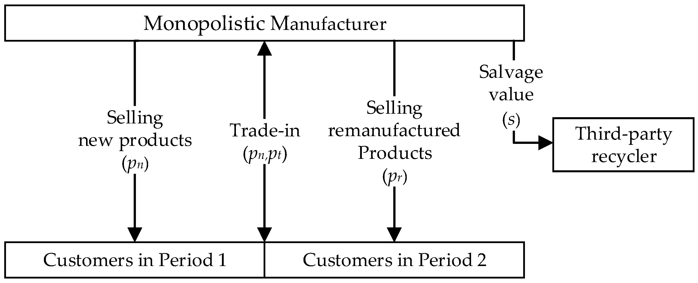
3.1. Model Description

This study considers a monopolistic manufacturer’s production, trade-in, and remanufacturing activities across two periods [3,16]. Electronics are typical examples. Leading electronics manufacturers like Apple and Lenovo have launched trade-in programs and sell remanufactured products through their official websites. In Period 1, the manufacturer produces new products and sells them at the unit price $p_n$, with the market size normalized to 1. New products purchased in Period 1 become used products after one usage period, transforming first-period buyers into used-product holders. In Period 2, the manufacturer continues producing new products at the unit price $p_n$ while implementing a trade-in program. The manufacturer offers a trade-in subsidy $p_t$ per unit of used product to customers participating in trade-in. During this period, the manufacturer can either remanufacture collected used products or resell them to third-party recyclers for residual value $s$ per unit of used product. The unit price of remanufactured products is $p_r$. Both periods’ new products have identical unit production costs $c_n$ ($0<c_n<1$) [13], while the unit remanufacturing cost is $c_r$, where $c_n>c_r$. In practice, manufacturers often prioritize pricing stability for flagship products (e.g., smartphones, appliances) to mitigate consumer dissatisfaction risks. A representative case is Apple’s pricing strategy: the iPhone 15 Plus was launched at GBP 799 in 2023, and its successor, the iPhone 16, retained the same GBP 799 price point in 2024. To balance price stability with circular economy goals, Apple simultaneously introduced trade-in rebates (e.g., up to GBP 4409 for the return of an iPhone 15 Plus) and sold remanufactured products (e.g., refurbished iPhone 15 Plus units priced at GBP 679). This dual approach aligns with that of De Giovanni and Zaccour [31], who modeled similar price stability.

This study assumes that $s$ is exogenous [14] and $p_t$ is uniform regardless of the used product quality [31,32]. The sales volumes of new products in Periods 1 and 2 are $q_{1n}$ and $q_{2n}$, respectively, with the quantity of used products collected through trade-in at the beginning of Period 2 denoted as $q_t$. The manufacturer’s remanufactured product sales volume is $q_r$. The process during the two periods is shown in Figure 1.

Based on whether the manufacturer commits to the price of remanufactured products in Period 1, we developed optimal decision-making models under two scenarios: trade-in without remanufacturing price commitment (TR) and trade-in with remanufacturing price commitment (CTR). The price announcements under the different scenarios are summarized in

Table 2. The manufacturer’s price announcements during each period in the two models.

Scenario	Price Announcement in Each Period
	First Period	Second Period
TR	$p_n$	$p_r$, $p_t$
CTR	$p_n$, $p_r$	$p_t$

.

3.2. Model Assumptions

This study assumes that each customer uses at most one product (new, used, or remanufactured) during the planning horizon [1,6]. Both new and existing customers exhibit heterogeneous willingness to pay (WTP) for new products, denoted by $\theta$, which follows a uniform distribution over the interval $\left[0,1\right]$ [3,26,33,34]. After one usage cycle, new products undergo quality or functional degradation. In Period 2, existing customers’ perceived value of the retained used products diminishes to ${\delta }_u\theta$, where ${\delta }_u$($0<{\delta }_u<1$) represents the valuation discount coefficient for used products [34]. The discount coefficient ${\delta }_u$ inversely correlates with trade-in participation: a higher ${\delta }_u$ indicates stronger customer preference for retaining used products (implying greater collection difficulty), while a lower ${\delta }_u$ signals higher return propensity. Although the manufacturer upgrades remanufactured products to the latest specification, consumers generally perceive them to be inferior to new products. Let ${\delta }_r$($0<{\delta }_r<1$) denote the WTP discount coefficient for remanufactured products [16,35], yielding consumers’ WTP for remanufactured products as ${\delta }_r\theta$. Key parameters and variables are summarized in

Table 3. Symbols for model-related parameters and variables.

Parameters
Symbol	Definition	Symbol	Definition
$c_n$	unit production cost (new product)	${\delta }_r$	customer valuation coefficient for remanufactured product
$c_r$	unit remanufacturing cost (remanufactured product)	${\delta }_u$	customer valuation discount coefficient for used product
$s$	residual value per unit of used product
Variables
Symbol	Definition	Symbol	Definition
$p_{in}$	unit price of new product in Period $i$	$q_r$	demand for remanufactured products in Period 2
$p_t$	trade-in subsidy per unit of used product	${\pi }_{in}$	profit from new products in Period i
$p_r$	unit price of remanufactured product	${\pi }_r$	profit from remanufactured products in Period 2
$q_{in}$	demand for new products in Period $i$	$C_t$	recycling cost
$q_t$	quantity of used products collected via trade-in	${\pi }_0$	total profit across both periods

, where superscript $i=1,2$ denotes the time period. ${\pi }_{in}=(p_n-c_n)q_{in}$, ${\pi }_r=(p_r-c_r)q_r$, $C_t=q_t{p}_t$, ${\pi }_t={\pi }_{1n}+{\pi }_{2n}+{\pi }_r-C_t$.

4. Model Analysis

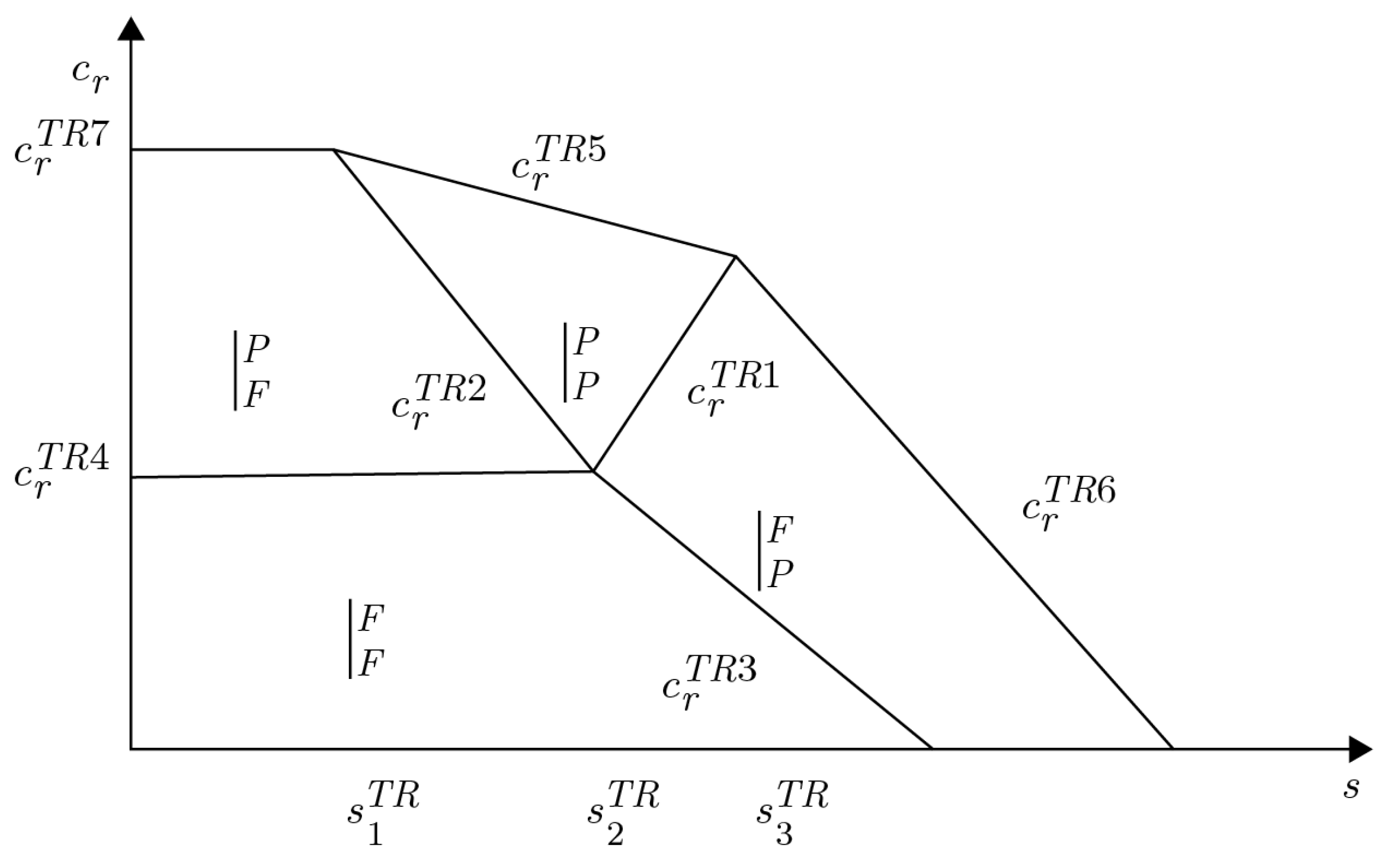
4.1. Trade-In Without Remanufactured-Product Price Commitment (TR Model)

In the TR model, the manufacturer announces $p_n$ in Period 1 and discloses prices $p_t$ and $p_r$ in Period 2. Because the manufacturer only announces the new-product price in Period 1, consumers make purchasing decisions in Period 1 solely based on the net utility of that period. If a consumer purchases the new product in Period 1, their net utility is $\theta -p_n$; if they do not purchase it, their net utility is 0. Consumers will purchase the new product in Period 1 if $\theta \ge p_n$, and abstain from purchasing otherwise. The demand function for new products in Period 1 is $q_{1n}^{TR}={\displaystyle {\int }_{p_n}^1}d\theta =1-p_n$.

Existing customers who purchased new products in Period 1 face distinct purchasing options in Period 2. If an existing customer participates in the trade-in program in Period 2, the net utility is $\theta -p_n+p_t$; if they continue to use the used product, the net utility is ${\delta }_u\theta$. A customer will adopt the trade-in strategy if $\theta -p_n+p_t>{\delta }_u\theta$ and $\theta >p_n$. Otherwise, they retain the used product. Under these conditions, the quantity of used products collected via trade-in in Period 2 is derived as $q_t^{TR}={\displaystyle {\int }_{\frac{p_n-p_t}{1-{\delta }_u}}^1}d\theta =1-{\displaystyle \frac{p_n-p_t}{1-{\delta }_u}}$.

Customers who do not purchase new products in Period 1 (denoted as $\theta <p_n$) face distinct purchasing options in Period 2. Since the new-product price remains unchanged across both periods, these customers will not purchase new products in Period 2. When a consumer purchases a remanufactured product in Period 2, the net utility becomes ${\delta }_r\theta -p_r$; when they purchase neither a new nor a remanufactured product, their net utility remains 0. Consumers will purchase remanufactured products in Period 2 if ${\delta }_r\theta -p_r>0$; otherwise, they will abstain from both options. This study focuses on a scenario where the manufacturer simultaneously sells new and remanufactured products in Period 2; thus, ${\displaystyle \frac{p_r}{{\delta }_r}}<p_n$ is assumed to ensure market segmentation. The demand quantity for remanufactured products in Period 2 can be formulated as $q_r^{TR}={\displaystyle {\int }_{\frac{p_r}{{\delta }_r}}^{p_n}}d\theta =p_n-{\displaystyle \frac{p_r}{{\delta }_r}}$. From the preceding analysis, it can be concluded that the sales volume of new products in Period 2 originates from existing customers participating in the trade-in program. Specifically, the sales volume of new products in Period 2 is given by $q_{2n}^{TR}=q_t^{TR}={\displaystyle {\int }_{\frac{p_n-p_t}{1-{\delta }_u}}^1}d\theta =1-{\displaystyle \frac{p_n-p_t}{1-{\delta }_u}}$.

The manufacturer makes optimal decisions across both periods to maximize the total profit, with the objective function formulated in Equation (1).

$$\begin{array}{l}{\pi }_0^{TR}(p_n,p_t,p_r)=q_{1n}(p_n-c_n)+q_{2n}(p_n-c_n)+q_r(p_r-c_r)-q_t{p}_t+(q_t-q_r)s\\ s.t.q_{1n}\ge q_t\ge q_r>0\end{array}$$

(1)

In Equation (1), the first and second terms represent the new-product sales profits in the first and second periods, respectively. The third term represents the profit from remanufactured products in Period 2. The fourth term represents the trade-in recycling cost in Period 2, and the fifth term represents the direct disposal income of used products. The constraint conditions are as follows: $q_{1n}\ge q_t$ indicates that the quantity of recycled products in Period 2 shall not exceed the sales volume in Period 1; $q_t\ge q_r$ indicates that the remanufacturing quantity in Period 2 shall not exceed the quantity of recycled used products; and $q_r>0$ indicates that the manufacturer sells remanufactured products in Period 2.

Proposition 1.

When the remanufacturing cost is relatively low ($c_r<\min \{c_r^{TR7},c_r^{TR5},c_r^{TR6}\}$), the manufacturer will engage in recycling and remanufacturing:

(1) 

When  $c_r<\min \{c_r^{TR4},c_r^{TR3}\}$, the manufacturer adopts a strategy of full recycling and full remanufacturing (${|}_F^F$);

(2) 

When  $c_r^{TR4}<c_r<\min \{c_r^{TR2},c_r^{TR7}\}$, the manufacturer adopts a strategy of partial recycling and full remanufacturing (${|}_F^P$);

(3) 

When  $\max \{c_r^{TR1},c_r^{TR2}\}<c_r<c_r^{TR5}$, the manufacturer adopts a strategy of partial recycling and partial remanufacturing (${|}_P^P$);

(4) 

When  $\max \{0,c_r^{TR3}\}<c_r<\min \{c_r^{TR1},c_r^{TR6}\}$, the manufacturer adopts a strategy of full recycling and partial remanufacturing (${|}_P^F$).10

Proof. 

See Appendix A. □

The optimal solution for the manufacturer is shown in

Table A1. The optimal solution for the TR model.

Strategy	${|}_{\mathit{P}}^{\mathit{P}}$	${|}_{\mathit{P}}^{\mathit{F}}$	${|}_{\mathit{F}}^{\mathit{P}}$	${|}_{\mathit{F}}^{\mathit{F}}$
$p_n^{T{R}^{\ast }}$	${\displaystyle \frac{2(1+c_n)-(c_r+s)}{4-{\delta }_r}}$	${\displaystyle \frac{4(1+c_n)-c_r-3s-2{\delta }_u}{8-{\delta }_r-4{\delta }_u}}$	$\begin{array}{l}{\displaystyle \frac{2(1-{\delta }_u)(1+c_n)}{4-4{\delta }_u+4{\delta }_r-{\delta }_r^2}}+\\ {\displaystyle \frac{{\delta }_r(3-{\delta }_u+c_n-c_r)}{4-4{\delta }_u+4{\delta }_r-{\delta }_r^2}}\end{array}$	$\begin{array}{l}{\displaystyle \frac{1+c_n}{2{\delta }_r-{\delta }_u+2}}+\\ {\displaystyle \frac{c_r+3{\delta }_r-{\delta }_u}{2(2{\delta }_r-{\delta }_u+2)}}\end{array}$
$p_t^{T{R}^{\ast }}$	$\begin{array}{l}{\displaystyle \frac{(s-c_r)+2{\delta }_u}{(4-{\delta }_r)}}+\\ {\displaystyle \frac{{\delta }_r(1+c_n-{\delta }_u-s)}{2(4-{\delta }_r)}}\end{array}$	${\displaystyle \frac{{\delta }_u(4c_n-c_r-2{\delta }_u-3s+4)}{8-{\delta }_r-4{\delta }_u}}$	$\begin{array}{l}{\displaystyle \frac{({\delta }_r^2+2{\delta }_u)(1-{\delta }_u)}{4-4{\delta }_u+4{\delta }_r-{\delta }_r^2}}+\\ {\displaystyle \frac{2{\delta }_r{\delta }_u+{\delta }_r(2-{\delta }_u)c_n}{4-4{\delta }_u+4{\delta }_r-{\delta }_r^2}}-\\ {\displaystyle \frac{(2+{\delta }_r-2{\delta }_u)c_r}{4-4{\delta }_u+4{\delta }_r-{\delta }_r^2}}\end{array}$	$\begin{array}{l}{\displaystyle \frac{{\delta }_u(1+c_n)}{(2{\delta }_r-{\delta }_u+2)}}+\\ {\displaystyle \frac{{\delta }_u(c_r+3{\delta }_r-{\delta }_u)}{2(2{\delta }_r-{\delta }_u+2)}}\end{array}$
$p_r^{T{R}^{\ast }}$	$\begin{array}{l}{\displaystyle \frac{{\delta }_r(1+c_n)}{4-{\delta }_r}}+\\ {\displaystyle \frac{(2-{\delta }_r)(c_r+s)}{4-{\delta }_r}}\end{array}$	$\begin{array}{l}{\displaystyle \frac{c_r(4-{\delta }_r-2{\delta }_u)}{8-{\delta }_r-4{\delta }_u}}+\\ {\displaystyle \frac{{\delta }_r(2+2c_n-{\delta }_u)}{8-{\delta }_r-4{\delta }_u}}+\\ {\displaystyle \frac{2(2-{\delta }_r-{\delta }_u)s}{8-{\delta }_r-4{\delta }_u}}\end{array}$	$\begin{array}{l}{\displaystyle \frac{{\delta }_r{c}_r(2-{\delta }_r)}{4-4{\delta }_u+4{\delta }_r-{\delta }_r^2}}+\\ {\displaystyle \frac{{\delta }_r({\delta }_r+2c_n)(2-{\delta }_u)}{4-4{\delta }_u+4{\delta }_r-{\delta }_r^2}}\end{array}$	${\displaystyle \frac{{\delta }_r(2c_n+c_r+{\delta }_r)}{2{\delta }_r-{\delta }_u+2}}$
$q_{1n}^{T{R}^{\ast }}$	${\displaystyle \frac{2(1-c_n)+(c_r+s)-{\delta }_r}{4-{\delta }_r}}$	$\begin{array}{l}{\displaystyle \frac{4-4c_n+c_r}{8-{\delta }_r-4{\delta }_u}}+\\ {\displaystyle \frac{3s-{\delta }_r-2{\delta }_u}{8-{\delta }_r-4{\delta }_u}}\end{array}$	$\begin{array}{l}{\displaystyle \frac{2(1-{\delta }_u)(1-c_n)}{4-4{\delta }_u+4{\delta }_r-{\delta }_r^2}}+\\ {\displaystyle \frac{{\delta }_r(1+{\delta }_u-{\delta }_r+c_r-c_n)}{4-4{\delta }_u+4{\delta }_r-{\delta }_r^2}}\end{array}$	${\displaystyle \frac{2(1-c_n)-c_r+{\delta }_r-{\delta }_u}{2(2+2{\delta }_r-{\delta }_u)}}$
$q_{2n}^{T{R}^{\ast }}$	${\displaystyle \frac{1-{\delta }_u+s-c_n}{2(1-{\delta }_u)}}$	$\begin{array}{l}{\displaystyle \frac{4-4c_n+c_r}{8-{\delta }_r-4{\delta }_u}}+\\ {\displaystyle \frac{3s-{\delta }_r-2{\delta }_u}{8-{\delta }_r-4{\delta }_u}}\end{array}$	$\begin{array}{l}{\displaystyle \frac{{\delta }_r(1+c_n)}{4-4{\delta }_u+4{\delta }_r-{\delta }_r^2}}+\\ {\displaystyle \frac{2(1-{\delta }_u-c_n-c_r)}{4-4{\delta }_u+4{\delta }_r-{\delta }_r^2}}\end{array}$	${\displaystyle \frac{2(1-c_n)-c_r+{\delta }_r-{\delta }_u}{2(2+2{\delta }_r-{\delta }_u)}}$
$q_r^{T{R}^{\ast }}$	${\displaystyle \frac{{\delta }_r(1+c_n)-2(s+c_r)}{(4-{\delta }_r){\delta }_r}}$	$\begin{array}{l}{\displaystyle \frac{2(1+c_n)-{\delta }_u-s}{(8-{\delta }_r-4{\delta }_u)}}-\\ {\displaystyle \frac{2(2-{\delta }_u)(c_r+s))}{{\delta }_r(8-{\delta }_r-4{\delta }_u)}}\end{array}$	$\begin{array}{l}{\displaystyle \frac{{\delta }_r(1+c_n)}{4-4{\delta }_u+4{\delta }_r-{\delta }_r^2}}+\\ {\displaystyle \frac{2(1-{\delta }_u-c_n-c_r)}{4-4{\delta }_u+4{\delta }_r-{\delta }_r^2}}\end{array}$	${\displaystyle \frac{2(1-c_n)-c_r+{\delta }_r-{\delta }_u}{2(2+2{\delta }_r-{\delta }_u)}}$

of Appendix B.

The sale of remanufactured products and the disposal of used products are both sources of profit for the manufacturer that stem from recycling used products. Therefore, as illustrated in Figure 2, $c_r$ and $s$ jointly influence the manufacturer’s choice of four different types of recycling and remanufacturing strategies. The boundary relationships of $c_r$ for different recycling and remanufacturing strategies are shown in Figure 2. Among them, $s_1^{TR}={\delta }_u-1+c_n$, $s_2^{TR}={\displaystyle \frac{(2{\delta }_u+{\delta }_r)c_n-{\delta }_r(1-{\delta }_u)}{2+{\delta }_r}}$, and $s_3^{TR}={\delta }_u{c}_n$. The four recycling and remanufacturing strategies deduced in this study share certain similarities with Li et al.’s work [35]. While their analysis primarily investigates the conditions for adopting these four strategies from the perspective of $c_n$, this paper places greater emphasis on explaining manufacturers’ strategic choices through the lens of $c_r$ and $s$. Proposition 1 indicates the following:

(1) The condition required for the manufacturer to adopt remanufacturing is $c_r<\min \{c_r^{TR5},c_r^{TR6},c_r^{TR7}\}$. When $s$ is relatively small ($s<s_1^{TR}$), the residual value of used products is not attractive enough, and the manufacturer does not consider reselling used products. Therefore, as the critical point for remanufacturing, $c_r^{TR7}$ is independent of $s$. When $s$ is relatively large ($s>s_1^{TR}$), the manufacturer may resell the used products. The larger $s$ is, the more inclined the manufacturer is to dispose of the used products, and the lower the critical point ($\min \{c_r^{TR5},c_r^{TR6}\}$) is for adopting remanufacturing, which makes it less likely that the manufacturer will adopt the remanufacturing strategy.

(2) $s=\max \{s_4^{TR},s_5^{TR}\}$11 is the critical residual value line required for the manufacturer to adopt partial-remanufacturing and full-remanufacturing strategies. When $s$ is not attractive enough ($s<\max \{s_4^{TR},s_5^{TR}\}$), the manufacturer does not consider reselling the used products, and instead adopts a full-remanufacturing strategy. In particular, if $c_r$ is sufficiently small ($c_r<c_r^{TR4}$), the manufacturer recycles all the used products for full remanufacturing. When $s$ is relatively attractive ($s>\max \{s_4^{TR},s_5^{TR}\}$), the manufacturer resells some of the used products. $s=\max \{s_4^{TR},s_5^{TR}\}$ decreases with $c_r$, which indicates that the lower the remanufacturing cost $c_r$ is, the more attractive $s$ must be for the manufacturer to consider reselling the used products.

(3) When $s<s_3^{TR}$, $c_r=\max \{c_r^{TR1},c_r^{TR4}\}$ represents the critical threshold for manufacturers to adopt partial-recycling versus full-recycling strategies. When $c_r$ is relatively small ($c_r<\max \{c_r^{TR1},c_r^{TR4}\}$), the manufacturer exhibits higher remanufacturing motivation and implements full recycling. Conversely, they adopt partial recycling when $c_r$ is large. When $s$ is relatively small ($s<s_2^{TR}$), the critical threshold for a manufacturer’s recycling strategy ($c_r^{TR4}$) remains independent of $s$. When $s$ becomes sufficiently large ($s>s_2^{TR}$), the higher $s$ value increases the manufacturer’s recycling motivation, consequently relaxing the critical threshold for full recycling ($\partial c_r^{TR1}{\displaystyle /}\partial s>0$). When $s>s_3^{TR}$, $s$ becomes sufficiently attractive, and the manufacturer implements full recycling regardless of $c_r$.

Corollary 1.

(1) When $s>s_6^{TR}$, $s-p_t^{{TR}^{\ast }}>0$; otherwise, $s-p_t^{{TR}^{\ast }}\le 0$. (2) When  $c_r<c_r^{TR}$, $p_r^{{TR}^{\ast }}-p_t^{{TR}^{\ast }}-c_r>0$; otherwise,  $p_r^{{TR}^{\ast }}-p_t^{{TR}^{\ast }}-c_r\le 0$.

Corollary 1 indicates that the manufacturer does not always profit from the reuse of used products. The manufacturer can obtain profit by directly reselling the used products only when $s$ is sufficiently high; it can obtain profit by remanufacturing used products only when $s$ is sufficiently low.

Corollary 2.

The monotonicities of optimal solutions under different strategies in the TR model with respect to $c_n$, $c_r$, and $s$ are shown in 

Table 4. The monotonicities of optimal solutions under different strategies in the TR model with respect to $c_n$, $c_r$, and $s$.

Optimal Solutions	${\mathit{p}}_{\mathit{n}}^{{\mathit{T}\mathit{R}}^{\ast }}$		${\mathit{p}}_{\mathit{t}}^{\mathit{T}{\mathit{R}}^{\ast }}$		${\mathit{p}}_{\mathit{r}}^{\mathit{T}{\mathit{R}}^{\ast }}$		${\mathit{q}}_{1\mathit{n}}^{\mathit{T}{\mathit{R}}^{\ast }}$		${\mathit{q}}_{2\mathit{n}}^{\mathit{T}{\mathit{R}}^{\ast }}$		${\mathit{q}}_{\mathit{r}}^{\mathit{T}{\mathit{R}}^{\ast }}$
$c_n$	↑		↑		↑		↓		↓		${|}_P$	↑
											${|}_F$	↓
$c_r$	${|}^P$${|}_P^F$	↓	${|}^P$${|}_P^F$	↓	↑		${|}^P$${|}_P^F$	↑	${|}_P^P$	→	↓
									${|}_P^F$	↑
	${|}_F^F$	↑	${|}_F^F$	↑			${|}_F^F$	↓	${|}_F$	↓
$s$	${|}_P$	↓	${|}_P^P$	↑	${|}_P$	↑	${|}_P$	↑	${|}_P$	↑	${|}_P$	↓
			${|}_P^F$	↓
	${|}_F$	→	${|}_F$	→	${|}_F$	→	${|}_F$	→	${|}_F$	→	${|}_F$	→

Note: (1) ${|}^P$ and ${|}^F$ denote partial-recycling and full-recycling strategies, respectively; ${|}_P$ and ${|}_F$ represent partial-remanufacturing and full-remanufacturing strategies, respectively. (2) ↑ means monotonically increasing, → means irrelevant, and ↓ means monotonically decreasing.

.

Corollary 2 indicates that the monotonicity of optimal pricing and production quantities with respect to parameters $c_r$ or $s$ can vary under different strategies.

(1) The introduction of remanufactured products by the manufacturer in Period 2 serves to attract customers with a lower WTP in that period. When $c_r$ increases, the manufacturer’s incentive to remanufacture weakens, leading to reduced sales of remanufactured products and a greater focus on new products and reselling used products. Therefore, except for in the cases of full recycling and full remanufacturing (${|}_F^F$), the manufacturer lowers the prices of new products in Period 1 to stimulate sales. Under partial remanufacturing, the manufacturer also increases profit by reselling more recycled used products ($\partial (q_t^{T{R}^{\ast }}{|}_P-q_r^{T{R}^{\ast }}{|}_P){\displaystyle /}\partial c_r>0$). However, under full recycling and full remanufacturing (${|}_F^F$), since all first-period products are used for remanufacturing, the manufacturer must raise the price of new products to limit sales and, therefore, constrain the supply of used products.

(2) When $s$ is small, recycled products are not resold, and the manufacturer adopts a full-remanufacturing strategy (${|}_F$). In this case, the optimal pricing and production decisions are independent of $s$. As $s$ increases, once the manufacturer begins reselling some used products under the partial-remanufacturing strategy (${|}_P$), a higher $s$ increases the manufacturer’s incentive to recycle used products. Consequently, the manufacturer reduces the prices of new products to boost sales, potentially raising the trade-in subsidy, which collectively increase the volume of recycled used products. Meanwhile, sales of remanufactured products decline, while resales of used products rise.

(3) When $c_n$ increases, the manufacturer raises the prices of new products, the trade-in subsidy in Period 2, and the prices of remanufactured products. This results in reduced sales of new products across both periods and lower second-period recycling volumes. However, under partial remanufacturing, the quantity of remanufactured products increases with $s$, whereas under full remanufacturing, the quantity of remanufactured products decreases with $s$, due to constraints affecting the supply of recycled used products.

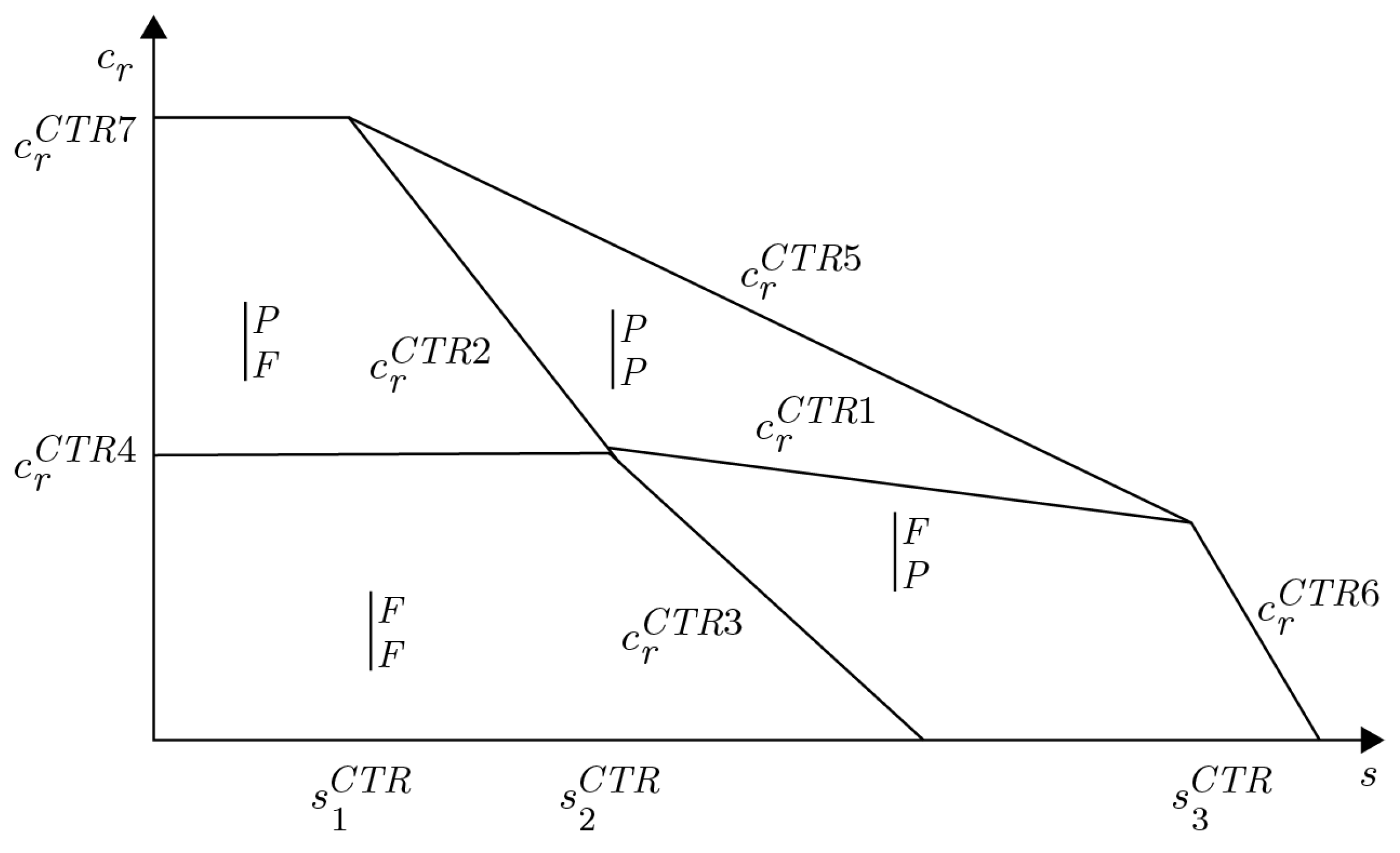
4.2. Trade-In with Remanufactured-Product Price Commitment (CTR Model)

In the CTR model, the manufacturer declares $p_n$, $p_r$ in Period 1, and $p_t$ in Period 2. Customers make their purchasing decisions in Period 1 based on the current pricing information ($p_n$ for new products and $p_r$ for remanufactured products). Because customers are informed in advance about the remanufactured product price, they conduct a utility comparison between two purchasing options: (1) buying a new product in Period 1; (2) postponing their purchase to acquire a remanufactured product in Period 2. This forward-looking decision-making process reflects how price commitment influences consumer behavior across different time periods. If a customer purchases the new product in Period 1, the net utility is $\theta -p_n$; if a customer purchases the remanufactured product in Period 2, the net utility is ${\delta }_r\theta -p_r$. When $\theta -p_n>{\delta }_r\theta -p_r$ and $\theta -p_n>0$, the customer purchases a new product in Period 1; otherwise, the customer does not make a purchase. The demand function for new products in Period 1 is $q_{1n}^{CTR}={\displaystyle {\int }_{\frac{p_n-p_r}{1-{\delta }_r}}^{1}d\theta =1}-{\displaystyle \frac{p_n-p_r}{1-{\delta }_r}}$.

The manufacturer announces $p_t$ in Period 2, and customers continue to make purchasing decisions related to price information. When $\theta -p_n+p_t>{\delta }_u\theta$ and $\theta >(p_n-p_r){\displaystyle /}(1-{\delta }_r)$, that is, $\theta >(p_n-p_t){\displaystyle /}(1-{\delta }_u)$, the customers participate in trade-in in Period 2; otherwise, they retain the used product. When ${\delta }_r\theta -p_r>0$ and $\theta <(p_n-p_r){\displaystyle /}(1-{\delta }_r)$, which is $p_r{\displaystyle /}{\delta }_r<\theta <(p_n-p_r){\displaystyle /}(1-{\delta }_r)$, the replacement customers purchase the remanufactured product in Period 2. $(p_n-p_r){\displaystyle /}(1-{\delta }_r)>p_r{\displaystyle /}{\delta }_r$ is assumed to ensure the existence of remanufactured products in Period 2. The quantities of trade-ins and sales of remanufactured products in Period 2 are derived as $q_t^{CTR}={\displaystyle {\int }_{\frac{p_n-p_t}{1-{\delta }_u}}^{1}d\theta }=1-{\displaystyle \frac{p_n-p_t}{1-{\delta }_u}}$, $q_r^{CTR}={\displaystyle {\int }_{\frac{p_r}{{\delta }_r}}^{\frac{p_n-p_r}{1-{\delta }_r}}d\theta }={\displaystyle \frac{p_n-p_r}{1-{\delta }_r}}-{\displaystyle \frac{p_r}{{\delta }_r}}$.

In brief, only existing customers will purchase the new product in Period 2, and the sales of the new product in Period 2 are indicated as $q_{2n}^{CTR}=q_t^{CTR}={\displaystyle {\int }_{\frac{p_n-p_t}{1-{\delta }_u}}^{1}d\theta }=1-{\displaystyle \frac{p_n-p_t}{1-{\delta }_u}}$.

Lemma 1.

When the manufacturer adopts the same $p_n$, $p_t$, and $p_r$ values in the two models and satisfies the assumptions of each model, $q_{1n}^{TR}>q_{1n}^{CTR}$, $q_t^{TR}=q_t^{CTR}$, $q_{2n}^{TR}=q_{2n}^{CTR}$, and $q_r^{TR}<q_r^{CTR}$; ${\pi }_{1n}^{TR}>{\pi }_{1n}^{CTR}$, ${\pi }_{2n}^{TR}={\pi }_{2n}^{CTR}$, ${\pi }_r^{TR}<{\pi }_r^{CTR}$, and ${\pi }_s^{TR}>{\pi }_s^{CTR}$.

In Period 1, the price commitment strategy for remanufactured products implemented by the manufacturer leads some customers with low WTP ($p_n<\theta <(p_n-p_r){\displaystyle /}(1-{\delta }_r)$) to delay purchasing the new product in Period 1; i.e., they purchase nothing in Period 1 and purchase the remanufactured product in Period 2. The remanufactured product and the new product participate in a similar contemporaneous race to the bottom. Therefore, compared to the TR model, the profit of new products falls in Period 1 (${\pi }_{1n}^{CTR}<{\pi }_{1n}^{TR}$), the profit of remanufactured products rises in Period 2 (${\pi }_r^{CTR}>{\pi }_r^{TR}$), the profit of new products remains unchanged in Period 2 (${\pi }_{2n}^{TR}={\pi }_{2n}^{CTR}$), and the profit from reselling used products decreases (${\pi }_s^{TR}>{\pi }_s^{CTR}$). The above analysis demonstrates that the manufacturer needs to weigh the effects of the various changes in the commitment of $p_r$ on the profit of new products, the profit of remanufactured products, and the profit of reselling used products in the CTR model.

The manufacturer makes optimal decisions in both periods simultaneously based on the maximization of total profits. The objective profit function is shown in Equation (2).

$$\begin{array}{l}{\pi }_0^{CTR}(p_n,p_t,p_r)=q_{1n}(p_n-c_n)+q_{2n}(p_n-c_n)+q_r(p_r-c_r)-q_t{p}_t+(q_t-q_r)s\\ s.t.q_{1n}\ge q_t\ge q_r>0\end{array}$$

(2)

Proposition 2.

When the remanufacturing cost is relatively low ($c_r<\min \{c_r^{CTR7},c_r^{CTR5},c_r^{CTR6}\}$), the manufacturer will engage in recycling and remanufacturing.

(1) 

When  $c_r<\min \{c_r^{CTR4},c_r^{CTR3}\}$, the manufacturer adopts a full-recycling and full-remanufacturing strategy (${|}_F^F$);

(2) 

When  $c_r^{CTR4}<c_r<\min \{c_r^{CTR2},c_r^{CTR7}\}$, the manufacturer enacts a partial-recycling and full-remanufacturing strategy (${|}_F^P$);

(3) 

When  $\max \{c_r^{CTR1},c_r^{CTR2}\}<c_r<c_r^{CTR5}$, the manufacturer implements a partial-recycling and partial-remanufacturing strategy (${|}_P^P$);

(4) 

When  $\max \{0,c_r^{CTR3}\}<c_r<\min \{c_r^{CTR1},c_r^{CTR6}\}$, the manufacturer adopts a full-recycling and partial-remanufacturing strategy (${|}_P^F$)12.

Proof. 

See Appendix A. □

The optimal solution for the manufacturer is shown in

Table A2. The optimal solution for the CTR model.

Strategy	${|}_{\mathit{P}}^{\mathit{P}}$	${|}_{\mathit{P}}^{\mathit{F}}$	${|}_{\mathit{F}}^{\mathit{P}}$	${|}_{\mathit{F}}^{\mathit{F}}$
$p_n^{CT{R}^{\ast }}$	${\displaystyle \frac{1+c_n}{2}}$	$\begin{array}{l}{\displaystyle \frac{(1-{\delta }_r)(2c_n-s+1)}{2(2-{\delta }_r-{\delta }_u)}}+\\ {\displaystyle \frac{(1-{\delta }_u)(1+c_r+s)}{2(2-{\delta }_r-{\delta }_u)}}\end{array}$	${\displaystyle \frac{1+c_n}{2}}$	$\begin{array}{l}{\displaystyle \frac{(2c_n+c_r)(1+{\delta }_r)}{2(3{\delta }_r-{\delta }_u+2)}}+\\ {\displaystyle \frac{2-{\delta }_u+{\delta }_r(3+{\delta }_u-{\delta }_r)}{2(3{\delta }_r-{\delta }_u+2)}}\end{array}$
$p_t^{CT{R}^{\ast }}$	${\displaystyle \frac{{\delta }_u+s}{2}}$	$\begin{array}{l}{\displaystyle \frac{2(1-{\delta }_u)(c_r+s+{\delta }_u)}{2(2-{\delta }_r-{\delta }_u)}}\\ +{\displaystyle \frac{({\delta }_r-{\delta }_u)(s-2c_n-{\delta }_u)}{2(2-{\delta }_r-{\delta }_u)}}\end{array}$	$\begin{array}{l}{\displaystyle \frac{{\delta }_r(1-{\delta }_r)(c_n+2{\delta }_u-1)}{2(-{\delta }_r^2+{\delta }_r-{\delta }_u+1)}}\\ +{\displaystyle \frac{(1-{\delta }_u)({\delta }_r{c}_n+{\delta }_u-c_r)}{2(-{\delta }_r^2+{\delta }_r-{\delta }_u+1)}}\end{array}$	$\begin{array}{l}{\displaystyle \frac{(2c_n+c_r)({\delta }_r+{\delta }_u)}{2(3{\delta }_r-{\delta }_u+2)}}+\\ {\displaystyle \frac{(2-{\delta }_u){\delta }_u-{\delta }_r(2+{\delta }_r-6{\delta }_u)}{2(3{\delta }_r-{\delta }_u+2)}}\end{array}$
$p_r^{CT{R}^{\ast }}$	${\displaystyle \frac{c_r+{\delta }_r+s}{2}}$	${\displaystyle \frac{c_r+{\delta }_r+s}{2}}$	$\begin{array}{l}{\displaystyle \frac{{\delta }_r{c}_r(1-{\delta }_r)}{2(-{\delta }_r^2+{\delta }_r-{\delta }_u+1)}}+\\ {\displaystyle \frac{{\delta }_r(c_n+{\delta }_r)(2-{\delta }_r-{\delta }_u)}{2(-{\delta }_r^2+{\delta }_r-{\delta }_u+1)}}\end{array}$	${\displaystyle \frac{{\delta }_r(2c_n+c_r+2{\delta }_r)}{3{\delta }_r-{\delta }_u+2}}$
$q_{1n}^{CT{R}^{\ast }}$	${\displaystyle \frac{1-c_n-{\delta }_r+s+c_r}{2(1-{\delta }_r)}}$	${\displaystyle \frac{1}{2}}-{\displaystyle \frac{2c_n-c_r-2s}{2(2-{\delta }_r-{\delta }_u)}}$	$\begin{array}{l}{\displaystyle \frac{(1-{\delta }_r-c_n)(1-{\delta }_u)}{2(-{\delta }_r^2+{\delta }_r-{\delta }_u+1)}}+\\ {\displaystyle \frac{+{\delta }_r(1-{\delta }_r+c_r)}{2(-{\delta }_r^2+{\delta }_r-{\delta }_u+1)}}\end{array}$	${\displaystyle \frac{-2c_n-c_r+{\delta }_r-{\delta }_u+2}{2(3{\delta }_r-{\delta }_u+2)}}$
$q_{2n}^{CT{R}^{\ast }}$	${\displaystyle \frac{1-{\delta }_u+s-c_n}{2(1-{\delta }_u)}}$	${\displaystyle \frac{1}{2}}-{\displaystyle \frac{2c_n-c_r-2s}{2(2-{\delta }_r-{\delta }_u)}}$	${\displaystyle \frac{1-{\delta }_u-c_r-(1-{\delta }_r)c_n}{2(-{\delta }_r^2+{\delta }_r-{\delta }_u+1)}}$	${\displaystyle \frac{-2c_n-c_r+{\delta }_r-{\delta }_u+2}{2(3{\delta }_r-{\delta }_u+2)}}$
$q_r^{CT{R}^{\ast }}$	${\displaystyle \frac{{\delta }_r{c}_n-(s+c_r)}{2{\delta }_r(1-{\delta }_r)}}$	${\displaystyle \frac{{\delta }_r(2c_n-s)-(2-{\delta }_u)(c_r+s)}{2{\delta }_r(2-{\delta }_r-{\delta }_u)}}$	${\displaystyle \frac{1-{\delta }_u-c_r-(1-{\delta }_r)c_n}{2(-{\delta }_r^2+{\delta }_r-{\delta }_u+1)}}$	${\displaystyle \frac{-2c_n-c_r+{\delta }_r-{\delta }_u+2}{2(3{\delta }_r-{\delta }_u+2)}}$

of Appendix B.

In the CTR model, the conditions compelling the manufacturer to choose diverse recycling and remanufacturing strategies are basically similar to those of the TR model. The boundary relationships of $c_r$ for different recycling and remanufacturing strategies are shown in Figure 3, in which $s_1^{CTR}={\delta }_u-1+c_n$, $s_2^{CTR}={\displaystyle \frac{({\delta }_u+{\delta }_r)c_n-{\delta }_r(1-{\delta }_u)}{1+{\delta }_r}}$, and $s_3^{CTR}={\delta }_u{c}_n$. The difference is that $c_r^{CTR1}$ decreases with $s$. In the CTR model, lower new-product sales in Period 1 are more likely to constrain the number of used products recycled in Period 2, so the manufacturer undertakes full recycling. When $s$ is relatively large ($s>s_2^{CTR}$), the manufacturer has a stronger incentive to recycle and resell the used product, and if $c_r$ is lower, a lower $p_r$ makes the remanufactured product a stronger competitor for the new product in Period 1, and the likelihood that the quantity recycled in Period 2 is constrained is greater. Therefore, as $s$ grows, the critical point for full recycling ($\min \{c_r^{CTR1},c_r^{CTR4}\}$) becomes smaller. In the TR model, when $s$ is larger, the manufacturer’s incentive to recycle and resell used products is likewise stronger. However, since remanufactured products only supplement the sales of new products in Period 1, the two approaches do not have a competitive predatory relationship, and remanufacturing and reselling are only two mutually complementary ways of reusing used products, the critical point $c_r^{CTR1}$ is even less restrictive as $s$ becomes larger, so full recycling is easier to achieve.

Concerning the analysis of the characteristics of the CTR model above, in the commitment of $p_r$, the remanufactured product exerts a cannibalization effect on new products in Period 1. For partial recycling, new products are all priced at $p_n^{\ast }{|}^P=(1+c_n){\displaystyle /}2$. For partial remanufacturing, the used product tackled for remanufacturing has a potential residual value ($s$) for resale, the actual cost of the remanufactured product is $c_r+s$, and the remanufactured product is priced at $p_r^{\ast }{|}_P=(c_r+{\delta }_r+s){\displaystyle /}2$. In particular, in the case of partially recycled and partially remanufactured products, a single cost-based pricing approach is adopted for both products ($p_n^{\ast }{|}_P^P=(1+c_n){\displaystyle /}2$, $p_r^{\ast }{|}_P^P=(c_r+{\delta }_r+s){\displaystyle /}2$).

Corollary 3.

(1) When $s<{\delta }_u$, $s-p_t^{CTR\ast }<0$; otherwise, $s-p_t^{CTR\ast }\ge 0$. (2) When $c_r<c_r^{CTR}$, $p_r^{CTR\ast }-p_t^{CTR\ast }-c_r>0$; otherwise, $p_r^{CTR\ast }-p_t^{CTR\ast }-c_r\le 0$. $c_r^{CTR}={\delta }_r-{\delta }_u$.

(1) Similarly to in the TR model, the manufacturer does not necessarily make positive profits from resale or remanufacturing. Under this condition, the manufacturer is more concerned with the promotional role of the recycling model for new products, and the reprocessing of used products is mainly treated as a method to cover the cost of recycling. With the commitment price $p_r$, remanufacturing is always unprofitable. (2) With a further commitment $p_r$ by the manufacturer, the remanufactured product conducts a race to the bottom with the new product in Period 1, and the manufacturer has more control over pricing $p_r$. The cost of obtaining a positive profit from remanufacturing ($c_r$) will become less demanding; therefore, $c_r^{CTR}>c_r^{TR}$.

Corollary 4.

The monotonicities of the optimal solutions under each strategy of the CTR model with respect to $c_n$, $c_r$, and $s$ are shown in 

Table 5. The monotonicities of optimal solutions under different strategies in the CTR model with respect to $c_n$, $c_r$, and $s$.

Optimal Solution	${\mathit{p}}_{\mathit{n}}^{{\mathit{C}\mathit{T}\mathit{R}}^{\ast }}$		${\mathit{p}}_{\mathit{t}}^{{\mathit{C}\mathit{T}\mathit{R}}^{\ast }}$		${\mathit{p}}_{\mathit{r}}^{{\mathit{C}\mathit{T}\mathit{R}}^{\ast }}$		${\mathit{q}}_{1\mathit{n}}^{{\mathit{C}\mathit{T}\mathit{R}}^{\ast }}$		${\mathit{q}}_{2\mathit{n}}^{{\mathit{C}\mathit{T}\mathit{R}}^{\ast }}$		${\mathit{q}}_{\mathit{r}}^{{\mathit{C}\mathit{T}\mathit{R}}^{\ast }}$
$c_n$	↑		${|}_P^P$	→	${|}_P$	→	↓		↓		${|}_P$	↑
			${|}_P^F$	↓							${|}_F$	↓
			${|}_F$	↑	${|}_F$	↑
$c_r$	${|}^P$	→	${|}_P^P$	→	↑		${|}^P$${|}_P^F$	↑	${|}_P^P$	→	↓
			${|}^F$	↑					${|}_P^F$	↑
	${|}^F$	↑	${|}_F^P$	↓			${|}_F^F$	↓	${|}_F$	↓
$s$	${|}_P^F$	↑	${|}_P$	↑	${|}_P$	↑	${|}_P$	↑	${|}_P$	↑	${|}_P$	↓
	${|}_P^P$${|}_F$	→	${|}_F$	→	${|}_F$	→	${|}_F$	→	${|}_F$	→	${|}_F$	→

Note: (1) ${|}^P$ and ${|}^F$ denote partial-recycling and full-recycling strategies, respectively, while ${|}_P$ and ${|}_F$ represent partial-remanufacturing and full-remanufacturing strategies, respectively. (2) ↑ means monotonically increasing, → means irrelevant, and ↓ means monotonically decreasing.

.

(1) With an increase in $c_r$, the manufacturer prefers to improve the pricing of remanufactured products. However, differently from the TR model, in the CTR model, when $c_r$ is sufficiently large and the manufacturer only adopts partial recycling, the manufacturer chooses to maintain the new-product price at $(1+c_n){\displaystyle /}2$ to increase the sales of new products in Period 1, focusing on ensuring profit through new-product sales in Period 1. Similarly, for partial remanufacturing, the quantity of remanufacturing is not constrained, and $p_r$ remains at $(c_r+{\delta }_r+s){\displaystyle /}2$, which is independent of $c_n$.

(2) Unlike in the TR model, in the CTR model, the monotonicity of $p_t$ with respect to $c_n$ does not always increase. For partial remanufacturing (${|}_P$), although the price of new products will increase with $c_n$, $p_t$ may decrease with $c_n$. This is due to the fact that in the CTR model, in Period 1, the manufacturer has already locked in the sales of new products and remanufactured products in Period 2 through $p_n$ and $p_r$; in Period 2, the manufacturer only announces $p_t$ to influence the quantity of trade-ins, thereby affecting the sales of new products and the profit on the resale of used products in Period 2. Regarding new-product sales, as $c_n$ increases, regardless of how $p_t$ changes, $q_{2n}^{CT{R}^{\ast }}$ ($q_t^{CT{R}^{\ast }}$) decreases. Because $p_t$ is the potential cost of reprocessing used products in Period 2, the actual unit net profit from the resale of used products is $s-p_t$. Once $s$ is sufficiently high ($s>$$\max \{s_4^{CTR},s_5^{CTR}\}$13), the manufacturer considers recycling and reselling used products. As $c_n$ increases, the manufacturer expects to maintain or reduce $p_t$ to keep, as far as possible, the net profit per unit gained from the resale of the used product ($s-p_t$). At the same time, while keeping $p_r$ unchanged, the net profit from refurbishing also increases ($(p_r-c_r-p_t)q_r$).

5. Model Comparison

Through the theoretical analysis of the two models above, it can be observed that $c_r$ and $s$ are critical parameters influencing the manufacturer’s choice of recycling and remanufacturing strategies, as well as the performance of optimal decisions and profits. The unit production cost of remanufactured products primarily includes unit material costs and other associated costs (e.g., labor, processing).

Under generalized $c_r$ and $s$ ($c_r>0$, $s>0$), it is theoretically challenging to define a common comparable interval for the two models to compare their optimal solutions. This study assumes that $c_r=s=0$. $c_r=0$ aligns with the prior literature on remanufacturing [35,36,37], where $s=0$ reflects the difficulty of monetizing the residual value of used products in the market [35,36,37]. Based on this assumption, we conducted theoretical analysis and numerical experiments to compare pricing, quantities, profits, and remanufacturing rates between the two models.

Lemma 2.

When  $c_r=s=0$, as  $c_n$  increases, the manufacturer will turn from a full-recycling and partial-remanufacturing strategy (${|}_P^F$) to a full-recycling and full-remanufacturing strategy (${|}_F^F$).

5.1. Optimal Prices

Corollary 5.

$p_n^{TR\ast }>p_n^{CTR\ast }$, $p_t^{TR\ast }>p_t^{CTR\ast }$, $p_r^{TR\ast }<p_r^{CTR\ast }$, $p_r^{TR\ast }-p_t^{TR\ast }-c_r<p_r^{CTR\ast }-p_t^{CTR\ast }-c_r$.

Corollary 5 shows that after the manufacturer commits to $p_r$, $p_n^{\ast }$ and $p_t^{\ast }$ both decrease, while $p_r^{\ast }$ increases. Under the commitment to $p_r$, the remanufactured products in Period 1 form a cannibalization relationship with the new products. On the one hand, the manufacturer lowers the price of new products and the trade-in subsidy; on the other hand, the manufacturer raises the price of remanufactured products. Compared to a scenario without price commitment, individual customers purchasing remanufactured products in Period 2 experience a reduced net utility (${\delta }_r\theta -p_r^{CT{R}^{\ast }}<{\delta }_r\theta -p_r^{T{R}^{\ast }}$). Furthermore, once this cannibalization relationship emerges, the manufacturer is more likely to achieve a positive net profit ($p_r-p_t-c_r$) from remanufacturing.

Furthermore, this study investigated the differential impacts of changes in the new product unit cost ($c_n$) on pricing decisions across two models through numerical experiments. The parameter values (${\delta }_r=0.7$, ${\delta }_u=0.5$) were selected based on dual rationales: (1) consistency with the prior literature (e.g., ${\delta }_r=0.7$ in [38,39] and ${\delta }_u=0.5$ in [40]); (2) alignment with practical observations. Enhanced remanufacturing capabilities and increasing promotional efforts have elevated consumer valuation coefficients for remanufactured products, as exemplified by Xiaomi’s remanufactured devices, which are priced at 65–75% of the price of new products14. ${\delta }_r=0.7$ reflects current market recognition of high-quality remanufactured goods while accommodating differentiated product strategies. Furthermore, ${\delta }_u=0.5$ is chosen to represent the median depreciation range across product categories, thereby strengthening the model’s generalizability to diverse market scenarios. In subsequent numerical experiments, this study adopts the same parameter combination.

Figure 4 validates the theoretical results of Corollary 5 and provides additional implications. Figure 4a,b reveal that the price gap between the two models in $p_n$ and $p_t$ exhibits a non-monotonic variation characteristic with respect to $c_n$: when $c_n$ is low, the gap widens as $c_n$ increases; however, when $c_n$ exceeds a critical threshold, the gap gradually diminishes with further increases in $c_n$. Figure 4c shows that the price gap in $p_r$ between the two models decreases monotonically as $c_n$ rises. Figure 4d shows that as $c_n$ increases, the unit profit advantage ($p_r-p_t$) derived from the price commitment for remanufactured products demonstrates a diminishing marginal pattern, indicating that cost pressures significantly suppress the marginal benefit of remanufacturing operations.

5.2. Optimal Quantities

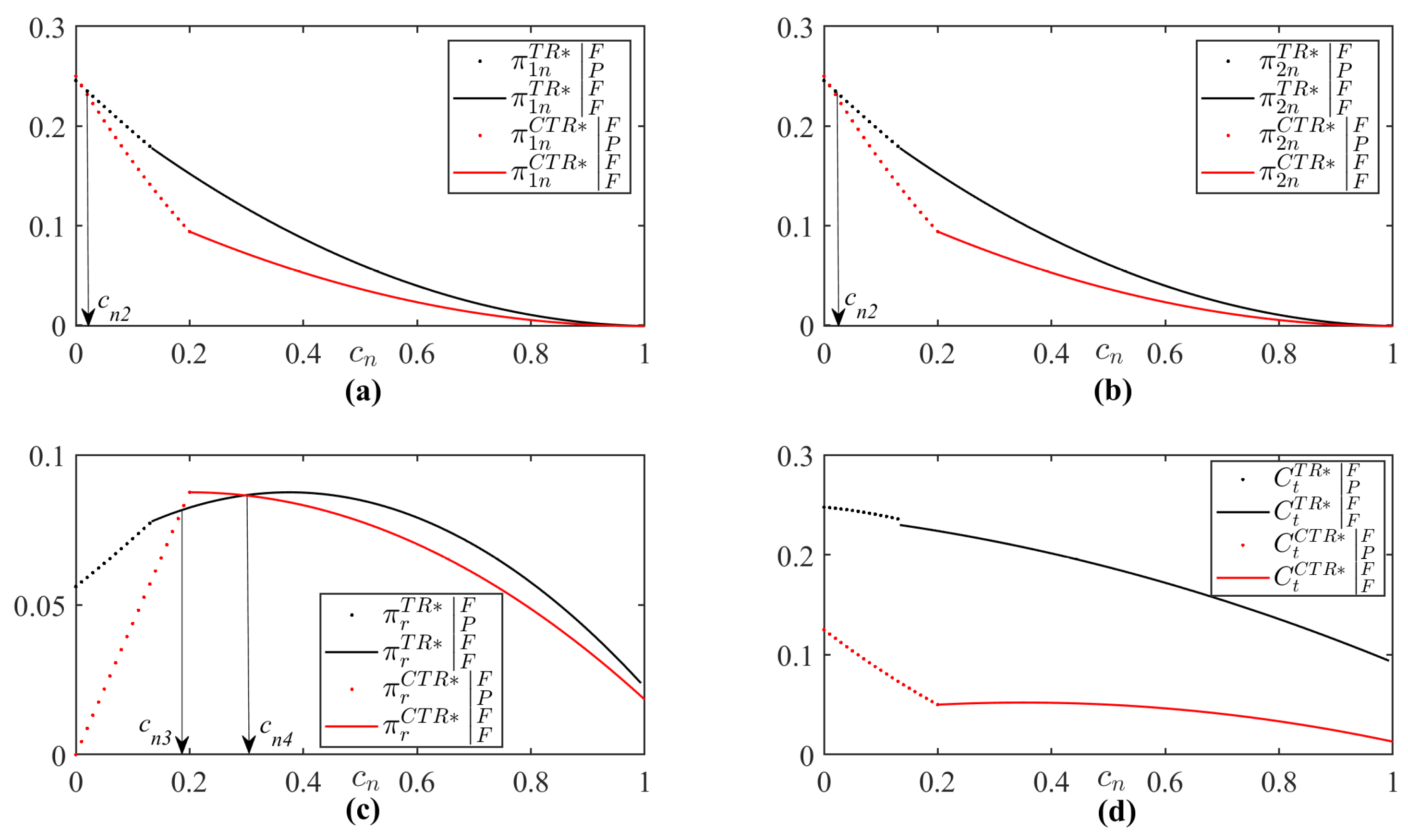
Corollary 6.

When $c_n<c_{n1}$,$q_{1n}^{TR\ast }<q_{1n}^{CTR\ast }$,$q_{2n}^{TR\ast }<q_{2n}^{CTR\ast }$,$q_t^{TR\ast }<q_t^{CTR\ast }$; otherwise,$q_{1n}^{TR\ast }>q_{1n}^{CTR\ast }$,$q_{2n}^{TR\ast }>q_{2n}^{CTR\ast }$,$q_t^{TR\ast }>q_t^{CTR\ast }$. $q_r^{TR\ast }>q_r^{CTR\ast }$. ${(q_{1n}+q_{2n}+q_r)}^{TR\ast }>{(q_{1n}+q_{2n}+q_r)}^{CTR\ast }$. $c_{n1}={\displaystyle \frac{2-{\delta }_r-{\delta }_u}{4}}$.

Corollary 6 shows that for products with relatively high unit production costs ($c_n>c_{n1}$), the manufacturer cannot increase the sales volume of new products in Period 1 by lowering $p_n$ after committing to $p_r$, because this causes some customers with low willingness to pay in Period 1 to consider purchasing products in Period 2. However, because the manufacturer has increased $p_r$, it loses some customers with low willingness to pay who would have purchased remanufactured products in Period 2, i.e., $q_r^{CTR\ast }<q_r^{TR\ast }$. Generally speaking, in the CTR model, the manufacturer does not gain an advantage in terms of either the second-period sales volume or the total sales volume over the two periods, i.e., ${(q_{1n}+q_{2n}+q_r)}^{T{R}^{\ast }}>{(q_{1n}+q_{2n}+q_r)}^{CT{R}^{\ast }}$.

Figure 5 not only verifies Corollary 6, but also offers additional insights. Figure 5a demonstrates that when $c_n<c_{n1}$, the discrepancy in $q_{1n}$ ($\left|q_{1n}^{T{R}^{\ast }}-q_{1n}^{CT{R}^{\ast }}\right|$) decreases as $c_n$ increases, whereas when $c_n>c_{n1}$, this discrepancy exhibits non-monotonic behavior. Figure 5b–d reveal that as $c_n$ increases, the differences between the two models in $q_r$, $q_{2n}+q_r$, and $q_{2n}+q_r+q_t$ gradually diminish. These experimental results indicate that when $c_n$ exceeds a critical threshold, the influence of the remanufacturing price commitment on sales volume and recycling quantity progressively weakens with further increases in $c_n$.

5.3. Profits

Corollary 7.

${\pi }_0^{T{R}^{\ast }}>{\pi }_0^{CT{R}^{\ast }}$.

Corollary 7 shows that remanufactured price commitment does not help to increase the total profit for the manufacturer in the two periods. As ${\pi }_0={\pi }_{1n}+{\pi }_{2n}+{\pi }_r-C_t$, and given the limitations of analytical methods in directly revealing the dynamics of ${\pi }_{1n}$, ${\pi }_{2n}$, ${\pi }_r$, and $C_t$ in the context of the two models, this study employed a numerical experiment to observe the results. This approach provides a robust interpretation of the comparative results for optimal profit between the two models.

As shown in Corollary 6, for products with a relatively low unit production cost ($c_n<c_{n1}$), lowering $p_n$ helps to increase the sales volume of new products in Period 1. Figure 6 shows that when $c_n$ is low enough ($c_n<c_{n2}<c_{n1}$), this promotional method is beneficial for increasing the profit of new products in Period 1 (${\pi }_{1n}$). However, as $c_n$ increases to become $c_{n1}$, this promotional profit advantage disappears. This indicates that when $c_n$ is low, the cost advantage of remanufacturing ($\left|0-c_n\right|$) is relatively unclear, and the manufacturer still attempts to ensure the profitability of new products in both periods (${\pi }_{1n}$ and ${\pi }_{2n}$) through pricing strategies.

Although committing to $p_r$ creates a competitive relationship between remanufactured products and new products in Period 1, the manufacturer’s strategy of raising prices causes the sales volume of remanufactured products ($q_r$) to decline. This changing trend makes the relationship between the magnitudes of ${\pi }_r$ in the two models more complex as $p_r$ increases. When $c_n$ is small enough ($c_n<c_{n3}$) or $c_n$ is large enough ($c_n>c_{n4}$), ${\pi }_r$ will decrease, and only when $c_n$ is moderate ($c_{n3}<c_n<c_{n4}$) can the manufacturer obtain higher profit from remanufactured products by committing to $p_r$.

The numerical experiments show that committing to $p_r$ does not always enable the manufacturer to obtain higher profit from remanufactured products, nor does it always cause the manufacturer to lose profit from new products. When $c_n$ is fixed, there is no situation in which the relationships between ${\pi }_{1n}$, ${\pi }_{2n}$, ${\pi }_r$, and $-C_t$ change consistently.

In summary, committing to $p_r$ in Period 1 triggers a cannibalization effect on the sales of new products in the same period. This reduces profits from new-product sales across both periods, thereby significantly impacting the trend in the manufacturer’s total profit. Consequently, the manufacturer cannot achieve higher profitability through price commitment.

Furthermore, this study observed the dynamics of profit reduction after price commitment through numerical experiments. Figure 7 shows that as $c_n$ increases, the gap in total profits between the two models ($\left|{\pi }_0^{T{R}^{\ast }}-{\pi }_0^{CT{R}^{\ast }}\right|$) gradually narrows.

5.4. Remanufacturing Rate

Corollary 8.

When $c_n<c_{n5}$, $(q_r{\displaystyle /}{q}_t{)}^{TR\ast }>(q_r{\displaystyle /}{q}_t{)}^{CTR\ast }$; otherwise, $(q_r{\displaystyle /}{q}_t{)}^{TR\ast }=(q_r{\displaystyle /}{q}_t{)}^{CTR\ast }$. $c_{n5}={\displaystyle \frac{2-{\delta }_r-{\delta }_u}{4}}$.

Corollary 8 shows that when $c_n$ is relatively small ($c_n<c_{n5}$), the manufacturer’s commitment to $p_r$ may instead decrease the remanufacturing rate. This is mainly because after the manufacturer raises $p_r$, $q_r$ decreases, which has a major impact on the overall decline in the remanufacturing rate.

The numerical experiment in Figure 8 shows that when $c_n<c_{n5}$, the gap in remanufacturing rates ($\left|(q_r{\displaystyle /}{q}_t{)}^{T{R}^{\ast }}-(q_r{\displaystyle /}{q}_t{)}^{CT{R}^{\ast }}\right|$) diminishes as $c_n$ increases. This indicates that for products with higher unit production costs, the influence of price commitment on the remanufacturing rate weakens progressively.

A growing number of 3C enterprises have developed formal business models for selling remanufactured products through official channels. This study focuses on leading companies within the 3C industry and analyzes pricing strategies by monitoring official website disclosures from 10 enterprises as shown in

Table 6. A list of 10 enterprises in the 3C industry.

Enterprise	Price Commitment	Enterprise	Price Commitment
Samsung	No	Cannon	No
Surface	No	Xiaomi	No
Huawei	No	Dji	Yes
Dell	No	EPSON	Yes
Lenovo	No	Apple	Yes

Notes: The website of each enterprise is shown in Table A3 of Appendix C.

. The findings reveal that 70% of the sampled firms (e.g., Dell, Samsung, Huawei) adopt a non-price-commitment strategy (i.e., refraining from publicly disclosing remanufactured product discount rates), while only 30% (e.g., Apple, which explicitly advertises up to 15% discounts) implement a price-commitment strategy for remanufactured goods. This pattern demonstrates that in the 3C remanufacturing sector—characterized by high standardization and rapid product iteration—most enterprises prioritize profit retention through strategic pricing opacity.

6. Conclusions and Management Insights

6.1. Conclusions

This study constructed a production decision-making model for a manufacturer with a monopoly in a two-period market in which the manufacturer produces new products in Period 1, and then recycles used products through trade-in, and simultaneously sells new and remanufactured products to customers, in Period 2. This study constructed two models, depending on whether the manufacturer commits to the price of remanufactured products in advance: a model without price commitment and a model with price commitment for remanufactured products. By obtaining the optimal solution for each model, this study determined the following: Regardless of whether the price of remanufactured products is committed to in advance, when the manufacturer implements remanufacturing, four potential recycling and remanufacturing strategies can be used. The factors influencing the manufacturer’s selection of these four strategies are mainly jointly affected by the unit residual value of the used products and the unit cost of the remanufactured products. The manufacturer will adopt the full recycling strategy only when the unit residual value of the used products is attractive enough, and the manufacturer will adopt the full remanufacturing strategy in both models only when the unit cost of remanufacturing is relatively low.

Furthermore, this study observed the optimal solutions, profit levels, and remanufacturing rates of the two models when the unit remanufacturing costs and the unit residual values of the used products are sufficiently low (i.e., both parameters are set to 0). The results of the model comparison show the following: (1) Price commitment for remanufactured products compels the manufacturer to simultaneously lower the price of new products and reduce the trade-in subsidy, while elevating the price of remanufactured products. This approach does not necessarily increase the sales volumes of new products in Period 1; instead, it reduces the sales volumes of remanufactured products in Period 2. As a result, the profit from new products in both periods declines, and the profit from remanufactured-product sales is not effectively increased, meaning that the manufacturer performs worse in terms of total profit over the two periods. (2) Committing to the price of remanufactured products in advance does not increase the remanufacturing rate.

6.2. Management Insights

To comprehensively utilize the theoretical findings of this study, management insights are put forward.

(1) Residual value and cost thresholds: Strategy adoption depends on the levels of these values. A high residual value makes full recycling attractive, while a low remanufacturing cost is crucial for full remanufacturing. Managers can assess strategy viability and plan operations accordingly, e.g., increasing the residual value through better design or reducing the remanufacturing cost by optimizing processes.

(2) Impact of price commitment on profits: Theoretical results in special cases show that advance price commitment for remanufactured products may harm overall profitability. Managers should be cautious, as this may reduce sales volumes and lower total profits. Alternative pricing strategies should be explored.

Avoiding unintended consequences of price commitment: Since price commitment does not increase the remanufacturing rate, manufacturers should seek other ways to improve it, such as marketing campaigns, improving product quality, or establishing partnerships.

This study focused on the centralized operation decision-making problem faced by monopolistic manufacturers. While the monopoly assumption provides analytical tractability for modeling centralized decision-making, there are multiple parties, such as retailers and third-party remanufacturers, involved in the recycling and reuse of used products, thus forming a multi-level, closed-loop supply-chain network. There are several critical dimensions in the real world: power asymmetry, competitive dynamics, and information decentralization in multi-echelon systems. Therefore, exploring interactions and collaborative strategies among diverse entities in multi-level closed-loop supply chains—building upon the understanding of sequential interactions gained from our two-period model—constitutes one vital extension pathway. Extending the analytical framework to multi-period dynamics represents another. Future work encompassing both dimensions will employ dynamic programming or simulation to investigate the intricate coordination requirements and long-term sustainability performance of such complex systems.

References

1. Guide, V.D.R.; Wassenhove, L.N. Managing product returns for remanufacturing. Prod. Oper. Manag. 2001, 10, 142–155. [Google Scholar] [CrossRef]
2. Östlin, J.; Sundin, E.; Björkman, M. Importance of closed-loop supply chain relationships for product remanufacturing. Int. J. Prod. Econ. 2008, 115, 336–348. [Google Scholar] [CrossRef]
3. Yin, R.; Li, H.; Tang, C.S. Optimal pricing of two successive-generation products with trade-in options under uncertainty. Decis. Sci. 2015, 46, 565–595. [Google Scholar] [CrossRef]
4. Cao, K.; Xu, X.; Bian, Y.; Sun, Y. Optimal trade-in strategy of business-to-consumer platform with dual-format retailing model. Omega 2019, 82, 181–192. [Google Scholar] [CrossRef]
5. Hu, S.; Zhu, S.X.; Fu, K. Optimal trade-in and refurbishment strategies for durable goods. Eur. J. Oper. Res. 2023, 309, 133–151. [Google Scholar] [CrossRef]
6. Tang, F.; Dai, Y.; Ma, Z.J.; Choi, T.M. Trade-in operations under retail competition: Effects of brand loyalty. Eur. J. Oper. Res. 2023, 310, 397–414. [Google Scholar] [CrossRef]
7. Dong, R.; Wang, N.; Jiang, B.; He, Q. Within-brand or cross-brand: The trade-in option under consumer switching costs. Int. J. Prod. Econ. 2023, 255, 108676. [Google Scholar] [CrossRef]
8. Dou, G.; Choi, T.M. Does implementing trade-in and green technology together benefit the environment? Eur. J. Oper. Res. 2021, 295, 517–533. [Google Scholar] [CrossRef]
9. Cao, K.; Choi, T. Optimal Trade-in Return Policies: Is it Wise to be Generous? Prod. Oper. Manag. 2022, 31, 1309–1331. [Google Scholar] [CrossRef]
10. Zhang, F.; Zhang, R. Trade-in Remaufacturing, Customer Purchasing Behavior, and Government Policy. Manuf. Serv. Oper. Manag. 2018, 20, 601–616. [Google Scholar] [CrossRef]
11. Zhao, S.; You, Z.; Zhu, Q. Quality choice for product recovery considering a trade-in program and third-party remanufacturing competition. Int. J. Prod. Econ. 2021, 240, 108239. [Google Scholar] [CrossRef]
12. Feng, L.; Li, Y.; Fan, C. Optimization of pricing and quality choice with the coexistence of secondary market and trade-in program. Ann. Oper. Res. 2020, 1–18. [Google Scholar] [CrossRef]
13. Ferrer, G.; Swaminathan, J.M. Managing New and Remanufactured Products. Manag. Sci. 2006, 52, 15–26. [Google Scholar] [CrossRef]
14. Ferguson, M.E.; Toktay, L.B. The Effect of Competition on Recovery Strategies. Prod. Oper. Manag. 2006, 15, 351–368. [Google Scholar] [CrossRef]
15. Ovchinnikov, A. Revenue and Cost Management for Remanufactured Products. Prod. Oper. Manag. 2011, 20, 824–840. [Google Scholar] [CrossRef]
16. Agrawal, V.V.; Atasu, A.; Van Ittersum, K. Remanufacturing, Third-Party Competition, and Consumers’ Perceived Value of New Products. Manag. Sci. 2015, 61, 60–72. [Google Scholar] [CrossRef]
17. Yan, W.; Xiong, Y.; Xiong, Z.; Guo, N. Bricks vs. clicks: Which is better for marketing remanufactured products? Eur. J. Oper. Res. 2015, 242, 434–444. [Google Scholar] [CrossRef]
18. Yan, X.; Chao, X.; Lu, Y.; Zhou, S.X. Optimal Policies for Selling New and Remanufactured Products. Prod. Oper. Manag. 2017, 26, 1746–1759. [Google Scholar] [CrossRef]
19. Zhou, Q.; Meng, C.; Yuen, K.F. Remanufacturing authorization strategy for competition among OEM, authorized remanufacturer, and unauthorized remanufacturer. Int. J. Prod. Econ. 2021, 242, 108295. [Google Scholar] [CrossRef]
20. Aviv, Y.; Pazgal, A. Optimal pricing of seasonal products in the presence of forward-looking consumers. Manuf. Serv. Oper. Manag. 2008, 10, 339–359. [Google Scholar] [CrossRef]
21. Cachon, G.P.; Feldman, P. Price commitments with strategic consumers: Why it can be optimal to discount more frequently … than optimal. Manuf. Serv. Oper. Manag. 2015, 17, 399–410. [Google Scholar] [CrossRef]
22. Correa, J.; Montoya, R.; Thraves, C. Contingent preannounced pricing policies with strategic consumers. Oper. Res. 2016, 64, 251–272. [Google Scholar] [CrossRef]
23. Chen, Y.; Jiang, B. Dynamic pricing and price commitment of new experience goods. Oper. Res. 2021, 30, 2752–2764. [Google Scholar] [CrossRef]
24. Dasu, S.; Tong, C. Dynamic pricing when consumers are strategic: Analysis of posted and contingent pricing schemes. Eur. J. Oper. Res. 2010, 204, 662–671. [Google Scholar] [CrossRef]
25. Papanastasiou, Y.; Savva, N. Dynamic pricing in the presence of social learning and strategic consumers. Mark. Sci. 2017, 63, 919–939. [Google Scholar] [CrossRef]
26. Zhang, Y.; Zhang, J. Strategic customer behavior with disappointment aversion customers and two alleviation policies. Int. J. Prod. Econ. 2017, 191, 170–177. [Google Scholar] [CrossRef]
27. Wang, H.; Guan, Z.; Dong, D.; Zhao, N. Optimal pricing strategy with disappointment-aversion and elation-seeking consumers: Compared to price commitment. Int. Trans. Oper. Res. 2019, 28, 2810–2840. [Google Scholar] [CrossRef]
28. Sheng, J.; Du, S.; Nie, T.; Zhu, Y. Dynamic pricing vs. pre-announced pricing in supply chain with consumer heterogeneity. Electron. Commer. Res. Appl. 2023, 62, 101311. [Google Scholar] [CrossRef]
29. Liu, J.; Zhai, X.; Chen, L. Optimal pricing strategy under trade-in program in the presence of strategic consumers. Omega 2019, 84, 1–17. [Google Scholar] [CrossRef]
30. Esenduran, G.; Lu, L.X.; Swaminathan, J.M. Buyback pricing of durable goods in dual distribution channels. Manuf. Serv. Oper. Manag. 2020, 22, 412–428. [Google Scholar] [CrossRef]
31. De Giovanni, P.; Zaccour, G. Optimal quality improvements and pricing strategies with active and passive product returns. Omega. 2018, 88, 248–262. [Google Scholar] [CrossRef]
32. Genc, T.S.; Giovanni, P.D. Optimal return and rebate mechanism in a closed-loop supply chain game. Eur. J. Oper. Res. 2018, 269, 661–681. [Google Scholar] [CrossRef]
33. Fan, X.; Guo, X.; Wang, S. Optimal collection delegation strategies in a retail-/dual-channel supply chain with trade-in programs. Eur. J. Oper. Res. 2022, 303, 633–649. [Google Scholar] [CrossRef]
34. Bai, X.; Choi, T.; Li, Y.; Sun, X. Implementing trade-in programs in the presence of resale platforms: Mode selection and pricing. Prod. Oper. Manag. 2023, 32, 3193–3208. [Google Scholar] [CrossRef]
35. Li, Y.; Feng, L.; Govindan, K.; Xu, F. Effects of a secondary market on original equipment manufactures’ pricing, trade-in remanufacturing, and entry decisions. Eur. J. Oper. Res. 2019, 279, 751–766. [Google Scholar] [CrossRef]
36. Zhou, Y.; Xiong, Y.; Jin, M. Less is more: Consumer education in a closed-loop supply chain with remanufacturing. Omega 2021, 101, 102259. [Google Scholar] [CrossRef]
37. Xiong, Y.; Li, G.; Zhou, Y.; Fernandes, K.; Harrison, R.; Xiong, Z. Dynamic pricing models for used products in remanufacturing with lost-sales and uncertain quality. Int. J. Prod. Econ. 2014, 147, 678–688. [Google Scholar] [CrossRef]
38. Atasu, A.; Sarvary, M.; Van Wassenhove, L.N. Remanufacturing as a marketing strategy. Manag. Sci. 2008, 10, 1731–1746. [Google Scholar] [CrossRef]
39. Li, W.; Wang, P.; Nie, K. Transnational remanufacturing decisions under carbon taxes and tariffs. Eur. J. Oper. Res. 2024, 312, 150–163. [Google Scholar] [CrossRef]
40. Huang, X.; Atasu, A.; Tereyagoglu, N.; Toktay, L.B. Lemons, trade-ins, and certified pre-owned programs. Manuf. Serv. Oper. Manag. 2023, 25, 737–755. [Google Scholar] [CrossRef]
Figure 1. A two-period model for a monopolistic manufacturer, with production, trade-in, and remanufacturing of used products.
Systems 13 00472 g001
Figure 2. The conditional intervals of the optimal strategies for the TR model.
Systems 13 00472 g002
Figure 3. The conditional intervals of the optimal strategies for the CTR model.
Systems 13 00472 g003
Figure 4. Optimal pricing comparison between the TR and CTR models based on numerical experiments. Notes: (ad) are the price comparisons between the TR and CTR models for p n , p t , p r , and ( p r p t c r ) , respectively.
Systems 13 00472 g004
Figure 5. Optimal quantity comparison between the TR and CTR models based on numerical experiments. Notes: (ad) are quantity comparisons between the TR and CTR models for q 1 n , q r , ( q 2 n + q r ) , and ( q 1 n + q 2 n + q r ) , respectively.
Systems 13 00472 g005
Figure 6. Profit and cost comparisons between the TR and CTR models, based on numerical experiments. Notes: (ad) are comparisons between the TR and CTR models for π 1 n , π 2 n , π r , and C t , respectively.
Systems 13 00472 g006
Figure 7. Total profit comparison between the TR and CTR models based on numerical experiments.
Systems 13 00472 g007
Figure 8. Remanufacturing rate comparison between the TR and CTR models based on numerical experiments.
Systems 13 00472 g008