Enhancing Extreme Learning Machine Robustness via Residual-Variance-Aware Dynamic Weighting and Broyden–Fletcher–Goldfarb–Shanno Optimization: Application to Metro Crowd Flow Prediction

Abstract

Aiming at the robustness problem of the extreme learning machine (ELM) in noisy and nonuniform data scenarios, this paper proposes an improved algorithm (BFGS-URWELM) that integrates uniform residual weighting and Broyden–Fletcher–Goldfarb–Shanno (BFGS) quasi-Newton optimization. This method introduces a sample weighting mechanism based on the target residual variance, dynamically adjusts the importance of training samples, and iteratively corrects the input weights and biases of the ELM in combination with the BFGS optimization strategy, effectively improving the prediction accuracy and stability of the model. The experiment is based on the passenger flow data of 80 subway stations and compares traditional machine learning algorithms, ensemble learning methods, and ELM variant models. The results show that BFGS-URWELM achieves 28.34, 0.3071, and 19.76 in the RMSE, MAPE, and MAE indicators, respectively, which are 19.9–33.5% higher than the baseline ELM. In addition, the residual distribution is more concentrated near the zero value, and the goodness of fit $R^2$ is improved to 0.96. The algorithm significantly reduces the prediction error under high-noise data and provides a highly robust solution for traffic flow prediction tasks.

1. Introduction

Urban rail transit has become the preferred mode of transportation for densely populated cities due to its large capacity, high speed, and high reliability [1]. The rapid growth of urban rail transit construction in many countries has induced a sharp increase in passenger flow, resulting in rail transit congestion and reduced service quality. Therefore, how to analyze and manage urban rail transit passenger flow, especially to grasp the short-term variation of passenger flow, has become an urgent problem that operators need to solve in order to improve the efficiency of urban rail transit, alleviate congestion, and improve service quality [2].

Methods for predicting short-term passenger flow in urban rail transit are generally categorized into classical statistical models and machine learning models. Traditional statistical approaches, which include models like autoregressive integrated moving average (ARIMA) and exponential smoothing, were prevalent in earlier applications. For instance, Ni et al. [3] employed a combination of linear regression and ARIMA to forecast short-term passenger flow in the New York subway. Jiao et al. [4] enhanced the conventional Kalman filter model by integrating an error coefficient, historical bias, and Bayesian combination to estimate short-term railway passenger numbers. Nevertheless, despite the inherently nonlinear nature of traffic data—largely due to fluctuations between free-flowing and congested traffic conditions—the efficacy and applicability of these models are constrained by their presumption of linear behavior [5,6]. As most statistical techniques rely on linear time series models, they fail to accommodate nonlinear variations in passenger flow, leading to significant errors in short-term forecasts [7]. Consequently, a range of advanced models and methods, such as machine learning models and neural networks, have been developed and utilized to address these challenges in traffic or passenger flow forecasting.

In order to solve nonlinear prediction problems, machine learning methods are widely used [8,9,10,11,12,13]. Xie et al. [14] developed a spatiotemporal dynamic graph relation learning model (STDGRL) to predict urban subway station flow, proposed a spatiotemporal node embedding representation module to capture the traffic patterns of different stations, adopted a dynamic graph relation learning module to learn the dynamic spatial relations between subway stations without a predefined graph adjacency matrix, and provided a transformer-based long-term relation prediction module for long-term subway flow prediction. Yin et al. [15] proposed a multi-temporal multi-graph neural network (MTMGNN) that aggregates recent and long-term information, extracts temporal features through a gated convolutional neural network, and extracts spatial features through a multi-graph neural network module. Xiao et al. [16] proposed a short-term subway passenger flow prediction model based on a neural network (NN), which uses multi-source data, such as smart card data, mobile phone data, and subway network data, and extracts spatial and temporal features inside and outside the subway system through a long short-term memory layer and a fully connected layer to improve the accuracy and stability of prediction. Experimental results showed that the model outperformed multiple baseline models on the Suzhou dataset, and the inclusion of mobile phone data further improved the accuracy of prediction. Machine learning methods, especially neural network algorithms have achieved some results in predicting the flow of subway passengers due to their powerful feature extraction and complex relationship modeling capabilities. However, the neighborhood expansion mechanism of graph neural networks causes the computational complexity to grow exponentially with the number of nodes. Other neural network algorithms also have the problems of time-consuming training and poor generalization ability.

The extreme learning machine (ELM) [17] as a single-hidden-layer feedforward neural network has emerged as a competitive alternative due to its remarkable computational efficiency and universal approximation capability. Unlike conventional neural networks requiring iterative backpropagation, the ELM randomly initializes hidden layer parameters and analytically determines output weights through Moore–Penrose generalized inverse, achieving rapid training speeds while avoiding local minima. Recent studies have demonstrated the ELM’s effectiveness in traffic prediction scenarios [18], where its shallow architecture facilitates real-time processing of streaming data. Zou et al. [19,20] proposed the backpropagation ELM (BP-ELM), which can dynamically allocate the most appropriate input parameters according to the current residual of the model during the process of adding hidden nodes, improve the quality of new nodes, accelerate convergence, improve model performance, and be used for traffic flow prediction, aiming to solve the problem that parameter tuning of traditional neural network prediction models is prone to fall into local minima. Yang et al. [18], proposed an ELM by combining Tent chaotic sequences and the residual correction method and introduced a DROP strategy to reduce the impact of randomness on traffic flow prediction and avoid the use of iterative methods for weight optimization. Based on the ELM algorithm, the ELM combined with the evolutionary algorithm was proposed for traffic flow prediction [21,22]. The original extreme learning machine (ELM) algorithm assumes that all training samples are equally important, which makes it perform poorly in dealing with noise and outliers that are common in passenger flow variations, especially when dealing with irregular passenger flow patterns caused by special events or equipment failures. In addition, the random assignment of input weights and biases in the ELM algorithm may lead to ill-conditioned hidden layer matrices, resulting in unstable predictions across different initialization trials. Although regularization techniques (such as ridge regression ELM) alleviate this problem to some extent, they do not address the fundamental problem of parameter sensitivity. TheELM and its variants show potential in traffic forecasting, but further research is needed in dimensions such as robustness.

Faced with the challenge of data uncertainty, improving the modeling capability of the ELM has always been the focus of researchers. Based on the principle of structural risk minimization and weighted least squares, a new regularized ELM algorithm, weighted regularized ELM (WRELM) [23], was proposed. This method significantly improves the generalization performance of the model in most cases without extending the training time. He et al. [24] designed a hierarchical ELM that uses multiple subnetwork groups to simultaneously perform dimensionality reduction and noise filtering to cope with high-dimensional noisy data. However, these improved methods based on outlier detection may mistakenly identify real data as anomalies, thereby destroying the original data structure and causing information loss. To solve this problem, researchers turned to modifying the objective function to enhance the robustness of the model. The mixture ELM algorithm [25] enhances the modeling capability and flexibility of complex noise by fusing the objective functions of Gaussian and Laplace distributions and solving them using EM and IRLS algorithms. However, the modeling process makes the algorithm more complicated.

Unlike the above work, this paper proposes a method of weighting residuals to improve the prediction ability of the ELM and uses BFGS quasi-Newton optimization for optimization. For data from different traffic nodes, with different residual weights, the residual-variance-aware dynamic weighting method can understand the traffic pattern in more detail. The specific contributions are as follows:

• Residual-Driven Adaptive Weighting: We develop a dynamic weighting mechanism that quantifies sample importance through residual variance analysis. Unlike fixed weighting strategies, our approach automatically assigns lower weights to samples with higher prediction uncertainty, effectively suppressing noise propagation through the network.
• BFGS-Optimized Parameter Space: A BFGS quasi-Newton framework is integrated to refine the randomly initialized ELM parameters. This second-order optimization strategy iteratively adjusts input weights and biases by approximating the Hessian matrix, significantly improving model stability while maintaining computational efficiency.
• Unified Learning Framework: The proposed method establishes a synergistic relationship between residual-based weighting and parameter optimization. The BFGS component utilizes weighted residuals to guide search directions, while the updated parameters generate more reliable residuals for subsequent weighting adjustments, creating a self-improving learning loop.

Comprehensive experiments on real-world AFC data from 80 metro stations demonstrate BFGS-URWELM’s superiority over 12 baseline models, including neural networks, ensemble learners, and ELM variants. Statistical analysis of the residuals reveals that our method reduces error variance by 38.7% compared to the standard ELM, with particularly notable improvements in handling abrupt flow changes during rush hours.

2. Principles of Algorithms

2.1. Uniform Residual Weighted Extreme Learning Machine (URWELM)

The extreme learning machine (ELM) is a single hidden layer feedforward neural network proposed by Huang Guangbin et al. [17] based on the Moore–Penrose (MP) generalized inverse matrix theory. It has strong nonlinear fitting capabilities and is distinguished by its efficient training process. Unlike traditional neural networks, the ELM eliminates the need for iterative parameter optimization by directly solving a set of linear equations. This single-step training process effectively avoids the common issue of backpropagation, such as convergence to local minima, and achieves superior generalization performance with remarkably fast convergence.

For any dataset comprising N samples $(X_j,t_j)$, where $j=1,2,\dots ,N$, the input vector $X_j={[x_{j1},x_{j2},\dots ,x_{jn}]}^{\top }\in {\mathbb{R}}^n$, the target vector $t_j={[t_{j1},t_{j2},\dots ,t_{jm}]}^{\top }\in {\mathbb{R}}^m$, and the activation function is $g\left(x\right)$, the number of hidden layer nodes is denoted as L. The ELM network model is defined as

$$\sum _{i=1}^L{\beta }_{i}g\left(W_i^{\top }{X}_j+b_i\right)=t_j,j=1,\dots ,N$$

(1)

where $W_i={[w_{i1},w_{i2},\dots ,w_{in}]}^{\top }$ represents the input weight of the i-th hidden layer neuron, $b_i$ is the bias of the i-th hidden layer neuron, ${\beta }_i$ is the output weight of the i-th hidden layer neuron, and $O_j$ is the output of the network for the j-th sample.

When the ELM model achieves a zero-error approximation of the target matrix, it satisfies the following condition:

$$\sum _{j=1}^N{O}_j-t_j=0,$$

(2)

and the ELM network model can be reformulated as

$$\sum _{i=1}^L{\beta }_{i}g(W_i^{\top }{X}_j+b_i)=t_j,j=1,\dots ,N.$$

(3)

To simplify the representation, the hidden layer output matrix H is introduced, reducing Equation (3) to the matrix form:

$$T=H\beta ,refeq:ELM-4$$

(4)

where

$$H(W_1,\dots ,W_L;b_1,\dots ,b_L;x_1,\dots ,x_N)={\left[\begin{array}{ccc}g(W_1·X_1+b_1)& \cdots & g(W_L·X_1+b_L)\\ ⋮& \ddots & ⋮\\ g(W_1·X_N+b_1)& \cdots & g(W_L·X_N+b_L)\end{array}\right]}_{N\times L},$$

$$\beta =\left[\begin{array}{c}{\beta }_1^{\top }\\ ⋮\\ {\beta }_L^{\top }\end{array}\right],T={\left[\begin{array}{c}{t}_1^{\top }\\ ⋮\\ t_N^{\top }\end{array}\right]}_{N\times m}.$$

Once the input weights $W_i$ and biases $b_i$ are randomly assigned, the hidden layer output matrix H is uniquely determined. The training process is thus transformed into solving the linear system $H\beta =T$. Based on the Moore–Penrose generalized inverse theory, the output weights $\beta$ can be directly computed as

$$\beta =H^{+}T,$$

(5)

where $H^{+}$ denotes the MP generalized inverse matrix of H. For most practical cases, the number of training samples N exceeds the number of hidden layer nodes L ($N>L$), allowing Equation (5) to be reformulated as

$$\beta ={\left(H^{\top }H\right)}^{-1}{H}^{\top }T.$$

(6)

This formulation highlights the efficiency of the ELM, as it leverages the direct solution of a linear system rather than iterative optimization, providing both computational speed and robustness in model training.

The Uniform Residual Weighted Extreme Learning Machine (URWELM) is an advanced variation of the ELM algorithm that is specifically designed to enhance robustness against noisy and nonuniform data distributions. Unlike the standard ELM, which assumes equal importance for all training samples, the URWELM introduces a weighting mechanism based on residual variance. This allows the model to assign different levels of importance to samples, significantly improving its performance in high-noise or heterogeneous data scenarios.

As in the ELM, the hidden layer output matrix H is computed as

$$H=g(WX+b),$$

(7)

where $W\in {\mathbb{R}}^{L\times n}$ is the input weight matrix, $b\in {\mathbb{R}}^L$ is the bias vector, and $g(·)$ represents the activation function.

The weighting mechanism leverages the variance of the target outputs T. The sample variance is defined as

$${\sigma }^2={\displaystyle \frac{1}{N-1}}\sum _{j=1}^N{\parallel T_j-\overline{T}\parallel }^2,\overline{T}={\displaystyle \frac{1}{N}}\sum _{j=1}^N{T}_j,$$

(8)

where $\overline{T}$ is the mean of the target outputs. Based on this variance, the weights $w_j$ for each sample are determined as inversely proportional to ${\sigma }^2$:

$$w_j={\displaystyle \frac{1}{{\sigma }^2}}.$$

(9)

The optimization objective in URWELM is to minimize the weighted squared error, which is defined as

$$\beta =arg\underset{\beta }{min}{\parallel W^{1/2}(H\beta -T)\parallel }_2^2,$$

(10)

where $W=\mathrm{diag}(w_1,w_2,\dots ,w_N)$ is a diagonal matrix of sample weights.

Expanding the weighted squared error term gives

$$\parallel W^{1/2}{(H\beta -T)\parallel }_2^2={(H\beta -T)}^{\top }W(H\beta -T).$$

(11)

The optimization problem can be solved by setting the gradient with respect to $\beta$ to zero:

$${\displaystyle \frac{\partial }{\partial \beta }}\left({(H\beta -T)}^{\top }W(H\beta -T)\right)=0.$$

(12)

$$2H^{\top }WH\beta -2H^{\top }WT=0.$$

(13)

Thus, the solution for $\beta$ is

$$\beta ={\left(H^{\top }WH\right)}^{-1}{H}^{\top }WT.$$

(14)

The final predicted outputs F are computed as

$$F=H\beta .$$

(15)

By incorporating this weighted optimization process, the URWELM effectively addresses the limitations of uniform sample importance in the standard ELM, achieving improved generalization and robustness in challenging data environments. The specific process is shown in Algorithm 1.

Algorithm 1 Uniform Residual Weighted Extreme Learning Machine (URWELM).

Require: ${\left\{(X_j,T_j)\right\}}_{j=1}^N$: Training data, L: Number of hidden nodes, $g(·)$: Activation function Ensure: $\beta$: Output weights, F: Predicted outputs  1: Step 1: Initialize the model  2: Randomly assign input weights $W\in {\mathbb{R}}^{L\times n}$ and biases $b\in {\mathbb{R}}^L$  3: Compute the hidden layer output matrix: $$H=g(WX+b)$$  4: Step 2: Compute weights based on residual variance  5: Calculate the mean of the target outputs: $$\overline{T}={\displaystyle \frac{1}{N}}\sum _{j=1}^N{T}_j$$  6: Compute the sample variance: $${\sigma }^2={\displaystyle \frac{1}{N-1}}\sum _{j=1}^N{\parallel T_j-\overline{T}\parallel }^2$$  7: Assign weights inversely proportional to the variance: $$w_j={\displaystyle \frac{1}{{\sigma }^2}},W=\mathrm{diag}(w_1,w_2,\dots ,w_N)$$  8: Step 3: Solve for output weights $\beta$  9: Minimize the weighted squared error: $$\beta =arg\underset{\beta }{min}{\parallel W^{1/2}(H\beta -T)\parallel }_2^2$$ 10: Compute the solution: $$\beta ={\left(H^{\top }WH\right)}^{-1}{H}^{\top }WT$$ 11: Step 4: Compute the final predicted outputs 12: Compute the network outputs: $$F=H\beta$$ 13: return  $\beta ,F$

2.2. Convergence Analysis of URWELM

Given N training samples ${\left\{(x_i,t_i)\right\}}_{i=1}^N$ with noise variances ${\left\{{\sigma }_i^2\right\}}_{i=1}^N$, the URWELM model with L hidden nodes computes the output weights $\beta$ as follows:

$$\beta =\underset{\beta }{arg\; min}\sum _{i=1}^N{\displaystyle \frac{1}{{\sigma }_i^2}}{\parallel h\left(x_i\right)\beta -t_i\parallel }^2,$$

(16)

where $h\left(x_i\right)=g(V{x}_i+b)$ is the hidden layer output for sample $x_i$, with the following procedures defined:

• $V\in {\mathbb{R}}^{L\times d}$: Input weights randomly initialized from any continuous distribution.
• $b\in {\mathbb{R}}^L$: Hidden layer biases randomly initialized.
• $g(·)$: Nonlinear bounded activation function.

Theorem 1 

(Existence and Uniqueness). For $L\le N$, the following are satisfied:

1. 

V and b are initialized from any continuous distribution.

2. 

$g:\mathbb{R}\to \mathbb{R}$ is nonlinear piecewise continuous.

Then, with probability 1,

$$H^{\top }WH\succ 0(\mathit{positive}\mathit{definite})$$

(17)

Therein, the following are defined:

• $H=[h{\left(x_1\right)}^{\top };\cdots ;h{\left(x_N\right)}^{\top }]\in {\mathbb{R}}^{N\times L}$
• $W=\mathit{diag}(1/{\sigma }_1^2,\dots ,1/{\sigma }_N^2)$

Proof. 

The proof contains key steps:

1. Full Column Rank of H: From the randomness in V and b, the matrix H has full column rank almost surely when $L\le N$ [17]. This is because the set of parameters $(V,b)$ that make H rank-deficient has a Lebesgue measure of 0 in the parameter space [26].

2. Positive Definiteness: For any $z\in {\mathbb{R}}^L\setminus \left\{0\right\}$,

$$\begin{array}{cc}\hfill z^{\top }\left(H^{\top }WH\right)z& =\sum _{i=1}^N{\displaystyle \frac{1}{{\sigma }_i^2}}{\left(h\left(x_i\right)z\right)}^2\hfill \\ \hfill & >0(\sin \mathrm{ce}H\mathrm{has}\mathrm{full}\mathrm{column}\mathrm{rank}\mathrm{and}{W}_{ii}>0)\hfill \end{array}$$

3. Existence and Uniqueness of $\beta$: The solution $\beta ={\left(H^{\top }WH\right)}^{-1}{H}^{\top }WT$ exists uniquely because $H^{\top }WH$ is invertible (positive definite). □

Lemma 1 

(Weighted Approximation Error). For bounded activation functions satisfying $\left|g\left(z\right)\right|\le C_g$, the approximation error satisfies the following:

$$\parallel W^{1/2}{(H\beta -T)\parallel }_2\le \sqrt{{\lambda }_{max}\left(W\right)}·{\displaystyle \frac{C_g{\parallel \beta \parallel }_1}{\sqrt{L}}}$$

(18)

where ${\lambda }_{max}\left(W\right)={max}_{1\le i\le N}1/{\sigma }_i^2$.

Proof. 

Using the universal approximation property of ELM [17],

$$\begin{array}{cc}\hfill {\parallel H\beta -T\parallel }_W& \le \parallel W^{1/2}{\parallel }_2·{\parallel H\beta -T\parallel }_2\hfill \\ \hfill & \le \sqrt{{\lambda }_{max}\left(W\right)}\left(\underset{\beta }{inf}{\parallel H\beta -T\parallel }_2\right)\hfill \\ \hfill & \le \sqrt{{\lambda }_{max}\left(W\right)}·{\displaystyle \frac{C}{\sqrt{L}}}(\mathrm{a}.\mathrm{s}.)\hfill \end{array}$$

where the last inequality follows from the ELM’s approximation rate. □

Theorem 2 

(URWELM Convergence). Under the conditions of Theorem 1 and Lemma 1, with probability 1, the following are satified:

1. 

The solution $\beta ={\left(H^{\top }WH\right)}^{-1}{H}^{\top }WT$ exists uniquely.

2. 

The weighted training error converges to its global minimum.

3. 

The generalization error satisfies

$${\mathbb{E}[\parallel H\beta -T\parallel }_W]=\mathcal{O}\left({\displaystyle \frac{1}{\sqrt{L}}}\right)$$

(19)

Proof. 

1. Existence and Uniqueness: Direct consequence of Theorem 1.

2. Global Optimality: The quadratic objective function

$$J\left(\beta \right)=\parallel W^{1/2}{(H\beta -T)\parallel }_2^2$$

(20)

has Hessian $2H^{\top }WH\succ 0$, guaranteeing strict convexity.

3. Error Bound: From Lemma 1 and the closed-form solution,

$$\begin{array}{cc}\hfill \mathbb{E}[\parallel H\beta -T{\parallel }_W]& \le \sqrt{{\lambda }_{max}\left(W\right)}{·\mathbb{E}[\parallel H\beta -T\parallel }_2]\hfill \\ \hfill & \le \sqrt{{\lambda }_{max}\left(W\right)}·\mathcal{O}(1/\sqrt{L})\hfill \end{array}$$

□

The analysis reveals three fundamental advantages of the URWELM:

• Adaptive Weighting: The W matrix automatically down-weights high-variance samples without affecting convexity.
• Computational Efficiency: Maintains the ELM’s $\mathcal{O}\left(N^{2}L\right)$ time complexity for $L\ll N$.
• Probabilistic Guarantees: The “probability 1” results hold for any continuous initialization, making the method robust to random seeds.

Remark 1. 

In practice, we recommend adding a small regularization term $\lambda I$ to $H^{\top }WH$ for numerical stability when ${\sigma }_i^2\to 0$.

2.3. URWELM Combined with BFGS

The BFGS quasi-Newton method is an optimization algorithm that employs an approximate matrix to replace the Hessian matrix, effectively avoiding the need to compute the second-order derivatives of the objective function. This circumvents the computational complexity associated with inverting the Hessian matrix in the classical Newton method, thereby improving computational efficiency. By utilizing a matrix $B_t^{-1}$ that does not involve second-order derivatives, the BFGS quasi-Newton method performs a line search along the direction $-B_t^{-1}{g}_t$, achieving comparable performance to Newton’s method with reduced computational cost.

Consider a quadratic objective function $f\left(x\right)$ with a constant Hessian matrix H. The goal is to construct an approximation $B_t^{-1}$ to $H^{-1}$ in the Newton method such that

$$B_{t+1}\Delta x_t=\Delta g_t\Rightarrow \Delta x_t=B_{t+1}^{-1}\Delta g_t,$$

(21)

where $\Delta g_t=g_{t+1}-g_t$ represents the gradient difference at two consecutive iterations.

The iterative update of $B_t$ is defined as

$$B_{t+1}=B_t+\Delta B_t,t=0,1,2,\dots ,$$

(22)

where the initial matrix $B_0$ is typically chosen as the identity matrix I. The key task in this method is to determine the correction matrix $\Delta B_t$ for each iteration. Substituting Equation (22) into Equation (21) yields

$$\Delta B_t\Delta x_t=\Delta g_t-B_t\Delta x_t,$$

(23)

which provides the necessary condition for updating $\Delta B_t$.

Assuming the correction matrix $\Delta B_t$ takes the following rank-2 form:

$$\Delta B_t={\displaystyle \frac{\Delta g_t\Delta g_t^{\top }}{\Delta g_t^{\top }\Delta x_t}}-{\displaystyle \frac{B_t\Delta x_t\Delta x_t^{\top }{B}_t}{\Delta x_t^{\top }{B}_t\Delta x_t}},$$

(24)

which ensures that $B_t$ remains positive definite.

Using the Sherman–Morrison formula, the inverse matrix $B_{t+1}^{-1}$ can be iteratively updated as

$$B_{t+1}^{-1}=B_t^{-1}-{\displaystyle \frac{B_t^{-1}\Delta g_t\Delta x_t^{\top }{B}_t^{-1}}{\Delta g_t^{\top }{B}_t^{-1}\Delta g_t}}+{\displaystyle \frac{\Delta x_t\Delta x_t^{\top }}{\Delta g_t^{\top }\Delta x_t}}.$$

(25)

The process of the BFGS quasi-Newton method is shown in Algorithm 2.

Algorithm 2 BFGS quasi-Newton method.

Require: Objective function $f:{\mathbb{R}}^n\to \mathbb{R}$, initial point $x_0$, tolerance tol, maximum iterations K Ensure: Approximate solution $x^{*}$, final gradient $g^{*}$  1: Step 1: Initialization  2: Set $k\leftarrow 0$  3: Initialize $x\leftarrow x_0$  4: Compute gradient: $g\leftarrow \nabla f\left(x\right)$  5: Initialize inverse Hessian approximation: $B^{-1}\leftarrow I$▹ Typically, the identity matrix is used  6: Step 2: Iterative Update  7: while $\parallel g\parallel >\mathrm{tol}$ and $k<K$ do  8:    Compute search direction: $p\leftarrow -B^{-1}g$  9:    Perform a line search to determine step size $\alpha$▹ Ensure sufficient decrease and curvature conditions are met 10:  Update the iterate: $x_{\mathrm{new}}\leftarrow x+\alpha p$ 11:  Compute new gradient: $g_{\mathrm{new}}\leftarrow \nabla f\left(x_{\mathrm{new}}\right)$ 12:  Calculate differences: $$\Delta x\leftarrow x_{\mathrm{new}}-x,\Delta g\leftarrow g_{\mathrm{new}}-g$$ 13:  Update the inverse Hessian approximation using the Sherman-Morrison formula: $$B_{\mathrm{new}}^{-1}=B^{-1}-{\displaystyle \frac{B^{-1}\Delta g\Delta g^{\top }{B}^{-1}}{\Delta g^{\top }{B}^{-1}\Delta g}}+{\displaystyle \frac{\Delta x\Delta x^{\top }}{\Delta g^{\top }\Delta x}}$$ 14:  Update variables: $$x\leftarrow x_{\mathrm{new}},g\leftarrow g_{\mathrm{new}},B^{-1}\leftarrow B_{\mathrm{new}}^{-1}$$ 15:  Increment iteration counter: $k\leftarrow k+1$ 16: end while 17: Step 3: Termination 18: return  $x,g$

The BFGS quasi-Newton method is particularly effective for unconstrained optimization problems due to its ability to achieve rapid convergence for symmetric quadratic loss functions. This study proposes applying the BFGS quasi-Newton method to optimize the input weights and hidden layer biases of the URWELM model. In this framework, the symmetric quadratic loss function serves as the fitness function for the optimization process.

The overall computational complexity of the standard ELM is roughly O($N^{2}L$). In order to further improve the robustness and prediction accuracy of the model, the BFGS-URWELM uses the BFGS method to iteratively update the input weights and biases. As a second-order approximation method, each iteration of the BFGS method involves an approximate update of the Hessian matrix. The computational cost of each iteration is related to the parameter dimension (usually O($L^2{(n+1)}^2$)), but since the BFGS method usually has a faster convergence speed, the overall number of iterations is often small. Although the overall training time of the BFGS-URWELM will increase compared to the standard ELM due to the introduction of iterative optimization, on large-scale datasets, if the number of hidden layer nodes is much smaller than the number of samples and the number of iterations and convergence criteria of BFGS are set reasonably, the additional computational overhead will not grow exponentially. In other words, the BFGS-URWELM can maintain high prediction accuracy and robustness while still having acceptable computational efficiency.

The BFGS method was chosen primarily for its balance between computational efficiency and robust convergence properties. Unlike traditional Newton methods that require explicit computation and inversion of the full Hessian matrix—which can be computationally expensive and numerically unstable—the BFGS method constructs an approximation of the inverse Hessian using only gradient information. This rank-2 update not only reduces computational overhead but also maintains the positive definiteness of the approximation, ensuring that the search direction is always a descent direction. Moreover, the superlinear convergence of the BFGS method makes it especially attractive for optimizing models like the URWELM, where the symmetric quadratic loss function provides a favorable landscape for rapid and stable convergence. This efficiency and robustness are key reasons why the BFGS method is preferred over other second-order methods in this context.

Under the condition of uniform residual weighting, the objective function adopts the standard quadratic form without additional weight distortion, and the BFGS quasi-Newton method is used to optimize the quadratic objective function. Assume that the objective function is as follows:

$$f\left(x\right)={\displaystyle \frac{1}{2}}{(x-x^{*})}^{\top }H(x-x^{*}),$$

(26)

where H is a positive symmetric matrix (constant Hessian), and $x^{*}$ is the global optimal solution. The proof is divided into two stages: first, the initial linear convergence is proved, and then the local superlinear convergence is analyzed.

Theorem 3 

(Local Superlinear Convergence). Let

$$f\left(x\right)={\displaystyle \frac{1}{2}}{(x-x^{*})}^{\top }H(x-x^{*})$$

under the assumption of exact line search (i.e., ${\alpha }_t=1$) and standard conditions ensuring positive definiteness and strong convexity, the BFGS quasi-Newton method exhibits local superlinear convergence, namely,

$$\underset{t\to \infty }{lim}{\displaystyle \frac{\parallel x_{t+1}-x^{*}\parallel }{\parallel x_t-x^{*}\parallel }}=0.$$

Proof. 

Define the error vector by

$$e_t=x_t-x^{*}.$$

Since

$$\nabla f\left(x\right)=H(x-x^{*})=H{e}_t,$$

the BFGS update is given by

$$x_{t+1}=x_t-{\alpha }_t{B}_t^{-1}\nabla f\left(x_t\right).$$

With the exact line search ${\alpha }_t=1$, it simplifies to

$$x_{t+1}=x_t-B_t^{-1}H{e}_t.$$

Thus, the error update becomes

$$\begin{array}{cc}\hfill e_{t+1}& =x_{t+1}-x^{*}\hfill \\ & =x_t-x^{*}-B_t^{-1}H{e}_t\hfill \\ & =e_t-B_t^{-1}H{e}_t.\hfill \end{array}$$

Introduce the error matrix for the Hessian inverse approximation as

$$E_t=B_t^{-1}-H^{-1}.$$

Then,

$$B_t^{-1}=H^{-1}+E_t,$$

and substituting into the error update gives

$$\begin{array}{cc}\hfill e_{t+1}& =e_t-(H^{-1}+E_t)H{e}_t\hfill \\ & =e_t-H^{-1}H{e}_t-E_{t}H{e}_t\hfill \\ & =e_t-e_t-E_{t}H{e}_t\hfill \\ & =-E_{t}H{e}_t.\hfill \end{array}$$

Taking norms on both sides results in

$$\parallel e_{t+1}\parallel \le \parallel E_t\parallel \parallel H\parallel \parallel e_t\parallel .$$

Next, consider the quasi-Newton condition used in the BFGS update:

$$B_{t+1}{s}_t=y_t,$$

where

$$s_t=x_{t+1}-x_t,y_t=\nabla f\left(x_{t+1}\right)-\nabla f\left(x_t\right).$$

For a quadratic function, since

$$y_t=H(x_{t+1}-x_t)=H{s}_t,$$

the quasi-Newton condition becomes

$$B_{t+1}{s}_t=H{s}_t.$$

In the ideal case when $B_t^{-1}=H^{-1}$, it immediately follows that $E_t=0$. In practice, with continuous updates based on the new information $(s_t,y_t)$, one can show (under the maintained positive definiteness, strong convexity of the objective function, and appropriate line search conditions such as exact line search or strong Wolfe conditions) that

$$\underset{t\to \infty }{lim}{E}_t=0.$$

Defining the convergence factor

$${\gamma }_t=\parallel E_t\parallel \parallel H\parallel ,$$

we have

$$\parallel e_{t+1}\parallel \le {\gamma }_t\parallel e_t\parallel$$

and, since

$$\underset{t\to \infty }{lim}{\gamma }_t=0,$$

it follows that

$$\underset{t\to \infty }{lim}{\displaystyle \frac{\parallel e_{t+1}\parallel }{\parallel e_t\parallel }}=0.$$

This exactly meets the definition of local superlinear convergence. □

3. Experiment and Analysis

To evaluate the effectiveness of the proposed algorithm, we conducted experiments on two types of datasets. First, five publicly available regression datasets from the UCI repository were used as benchmarks. The details of these datasets are summarized in

Table 1. UCI regression dataset.

Dataset	Sample Size	Feature Dimension
California Housing	20,640	8
Diabetes	442	10
Concrete	1030	8
Slump	103	7
Servo	167	4

. These datasets span a range of sample sizes and feature dimensions, providing a diverse evaluation scenario for regression tasks.

In addition, we employed a real-world dataset consisting of 24 days of Hangzhou Metro passenger flow data. This dataset was sampled at 5-min intervals from 1 January to 25 January 2019, covering 80 stations across three metro lines. Such high-frequency data capture the complex and dynamic behavior of urban transportation systems. An example of the metro passenger flow data is presented in Figure 1. The figure also illustrates the performance variation of our algorithm when different numbers of neurons were employed, highlighting its sensitivity to this key parameter.

All experiments were run on the Intel Xeon E5-2600 v4 processor which is produced by Intel Corporation in Santa Clara, California, United States and compiled using PyCharm in the Python 3.7 environment. Several evaluation criteria were used to evaluate these algorithms. Equations (27)–(29) present the formulas for the adopted evaluation criteria.

(1) Root Mean Square Error (RMSE):

$$\mathrm{RMSE}=\sqrt{{\displaystyle \frac{1}{n}}\sum _{i=1}^n{({\mu }_i-{\widehat{y}}_i)}^2}.$$

(27)

The root mean square error is the square root of the ratio between the projected value’s squared departure from the real value and the number of observations n. It calculates the difference between the expected and true values and is sensitive to data that contain outliers.

(2) Mean Absolute Error (MAE):

$$\mathrm{MAE}={\displaystyle \frac{1}{n}}\sum _{i=1}^n|{\mu }_i-{\widehat{y}}_i|.$$

(28)

Another frequent assessment criterion in regression issues is the MAE. It is frequently used to calculate the difference between forecasts and actual observations. Compared to the MSE, the MAE is less sensitive to outliers because it calculates the absolute value of the error, so the penalty is fixed for any degree of error.

(3) Mean Absolute Percentage Error (MAPE):

$$\mathrm{MAPE}=100\%\times {\displaystyle \frac{1}{n}}\sum _{i=1}^n\left|{\displaystyle \frac{y_i-{\widehat{y}}_i}{y_i}}\right|.$$

(29)

The MAPE is often used to calculate the difference between expected and actual observed values. Because the MAPE is more unbiased and equitable in comparison to the raw data, it is frequently employed as an assessment metric in algorithmic comparisons.

3.1. Performance of URWELM Combined with BFGS

To evaluate the performance of the proposed ELM-based algorithms, we conducted extensive experiments on five benchmark regression datasets from the UCI repository: California Housing, Diabetes, Concrete, Slump, and Servo. These datasets vary in sample size and feature dimension, offering a comprehensive assessment of the algorithms under different data conditions. The specific performance is shown in

Table 2. Performence of different ELM algorithms on UCI dataset.

Dataset	ELM			RWELM			URWELM			BFGS-URWELM
	RMSE	MAEP	MAE	RMSE	MAEP	MAE	RMSE	MAEP	MAE	RMSE	MAEP	MAE
California Housing	0.6515	0.2756	0.4646	0.6204	0.2692	0.4468	0.6106	0.2622	0.4369	0.5887	0.2425	0.4129
Diabetes	56.6198	0.3823	43.9656	54.7039	0.3901	43.3866	54.1143	0.3725	42.2957	52.2971	0.3560	39.7967
Concrete	8.2258	0.2164	6.4208	7.8129	0.2173	6.2644	7.6743	0.2231	6.2432	6.9450	0.1288	3.8462
Slump	7.0751	0.1348	4.9075	4.5351	0.1028	3.4858	2.5266	0.0451	1.6304	0.9514	0.0214	0.7423
Servo	1.7301	1.0927	1.2092	1.3918	0.9844	0.8739	0.9982	0.8375	0.7480	0.5400	0.4587	0.3455

.

Table 2 validates the superiority of the proposed BFGS-URWELM method over the standard ELM and its other variants. The integration of residual weighting with BFGS optimization notably enhanced the predictive performance, making it a robust solution for various regression tasks.

Next, this study used 80 subway stations for testing. In order to verify the optimization effect of consistent residual weighting and BFGS, 21 days of training data were collected, and 2 days of test data were collected. The original subway station passenger flow data are summarized in a 5-min sampling period using a seven-step sliding window. The passenger flow data of the first 35 min were used to predict the subway station passenger flow of the next 5 min. The optimization was verified by ablation experiments. Figure 2 shows the performance of different ELM algorithms on 80 different stations.

Figure 2 illustrates that the BFGS-URWELM algorithm exhibited superior prediction accuracy and demonstrated enhanced stability across tests conducted at various sites. While the URWELM generally outperformed the RWELM, it performed less effectively at one specific site. The BFGS algorithm refines the URWELM, significantly addressing this limitation and enhancing its overall prediction accuracy. From an experimental point of view, it shows that consistent residual weighting can effectively reduce the impact of random information in passenger flow and improve algorithm stability, and BFGS optimization further improved the prediction accuracy. The performance of each algorithm is shown in

Table 3. ELM algorithm performance under different optimization strategies.

Different ELM	Mean RMSE	Mean MAPE	Mean MAE
ELM	35.3802	0.4621	24.7924
RWELM	33.4569	0.4581	23.7144
URWELM	32.5040	0.4563	23.1073
BFGS-URWELM	28.3361	0.3071	19.7599

.

As shown in Table 3, applying consistent residual weighting enhanced the original ELM algorithm across all three metrics. Furthermore, when both consistent residual weighting and BFGS optimization were utilized together, the performance accuracy of the extreme learning machine was significantly improved. The RWELM and URWELM both enhanced the performance of the model. The RWELM yielded a steady but moderate enhancement, whereas the URWELM showed more notable improvements in the RMSE and MAE scores. The most substantial effect was observed with the BFGS-URWELM, outperforming other optimization strategies, which underscores its superior capability in parameter tuning and optimization searching.

The application of the BFGS-URWELM led to a notable enhancement in model performance. The RMSE decreased from 35.3802 for the unoptimized ELM to 28.3361, representing a reduction of approximately 19.9% that demonstrates the efficacy of the optimization strategy in minimizing prediction errors. The MAPE dropped from 0.4621 to 0.3071, marking an improvement of about 33.5%, which highlights a significant reduction in the prediction percentage error. Meanwhile, the MAE was reduced from 24.7924 to 19.7599, a decrease of roughly 20.3%, suggesting that the predicted results are more closely aligned with the actual values.

In order to objectively evaluate the generalization performance of the proposed algorithm, this study used the time series cross-validation method TimeSeriesSplit [27] to divide the dataset into five continuous time series subsets. This method strictly maintains the causal structure of time series data by ensuring that the training set time window always precedes the validation set through an innovative splitting strategy. This time series isolation mechanism can effectively avoid evaluation bias caused by future information leakage while simulating the application conditions in real scenarios where the model can only make predictions based on historical data. The specific performance is shown in the

Table 4. Performance of ELM algorithm with different optimization strategies in TimeSeriesSplit cross-validation.

Different ELM	Mean RMSE	Mean MAPE	Mean MAE
ELM	36.3917	0.5386	26.0183
RWELM	32.1323	0.4491	22.9885
URWELM	31.4592	0.4224	22.3533
BFGS-URWELM	28.2261	0.3027	19.7605

.

Based on the cross-validation results using TimeSeriesSplit shown in Table 4, the effectiveness of the optimization strategy is further validated. Under strict temporal isolation conditions, the baseline ELM exhibited an increase in the RMSE to 36.3917—an increase of 2.86% compared to the non-temporal validation environment (35.3802). In contrast, the BFGS-URWELM maintained stable performance throughout cross-validation. Its RMSE of 28.2261 differed only marginally (by 0.39%) from the noncross-validation result of 28.3361, thereby demonstrating strong robustness with respect to temporal dependencies. Furthermore, a vertical comparison reveals that the BFGS-URWELM achieved a 22.43% reduction in the RMSE (from 36.3917 to 28.2261) and a 43.80% improvement in the MAPE (from 0.5386 to 0.3027) relative to the baseline ELM. Notably, the increase in the MAPE for the URWELM under cross-validation (21.58%) was markedly higher than that observed under nontemporal validation (1.25%), suggesting that the temporal isolation mechanism is more sensitive in detecting the corrective impact of the residual weighting strategy on long-term prediction bias.

3.2. Analysis Residuals of BFGS-URWELM

In order to analyze the sensitivity of the BFGS-URWELM, the number of neurons was set to 8, 16, 32, 64, and 128. The performance with different numbers of neurons is shown in Figure 3. The results indicate that increasing the number of neurons enhanced the model’s fitting performance up to an optimal point. The RMSE decreased from the configuration with 8 neurons, reaching its lowest value at 64 neurons with a value of approximately 28.34 and then slightly increasing at 128 neurons to about 29.07. The MAPE showed a significant reduction from 0.39 with 8 neurons to 0.30 with 64 neurons, and it remained constant at 0.30 with 128 neurons. The MAE followed a similar trend, decreasing to a minimum of 19.76 at 64 neurons and then marginally rising to 19.88 at 128 neurons. Therefore, 64 neurons represent an optimal balance that achieves the best or near-best performance across all evaluation metrics while mitigating the potential overfitting and optimization instability associated with higher neuron counts.

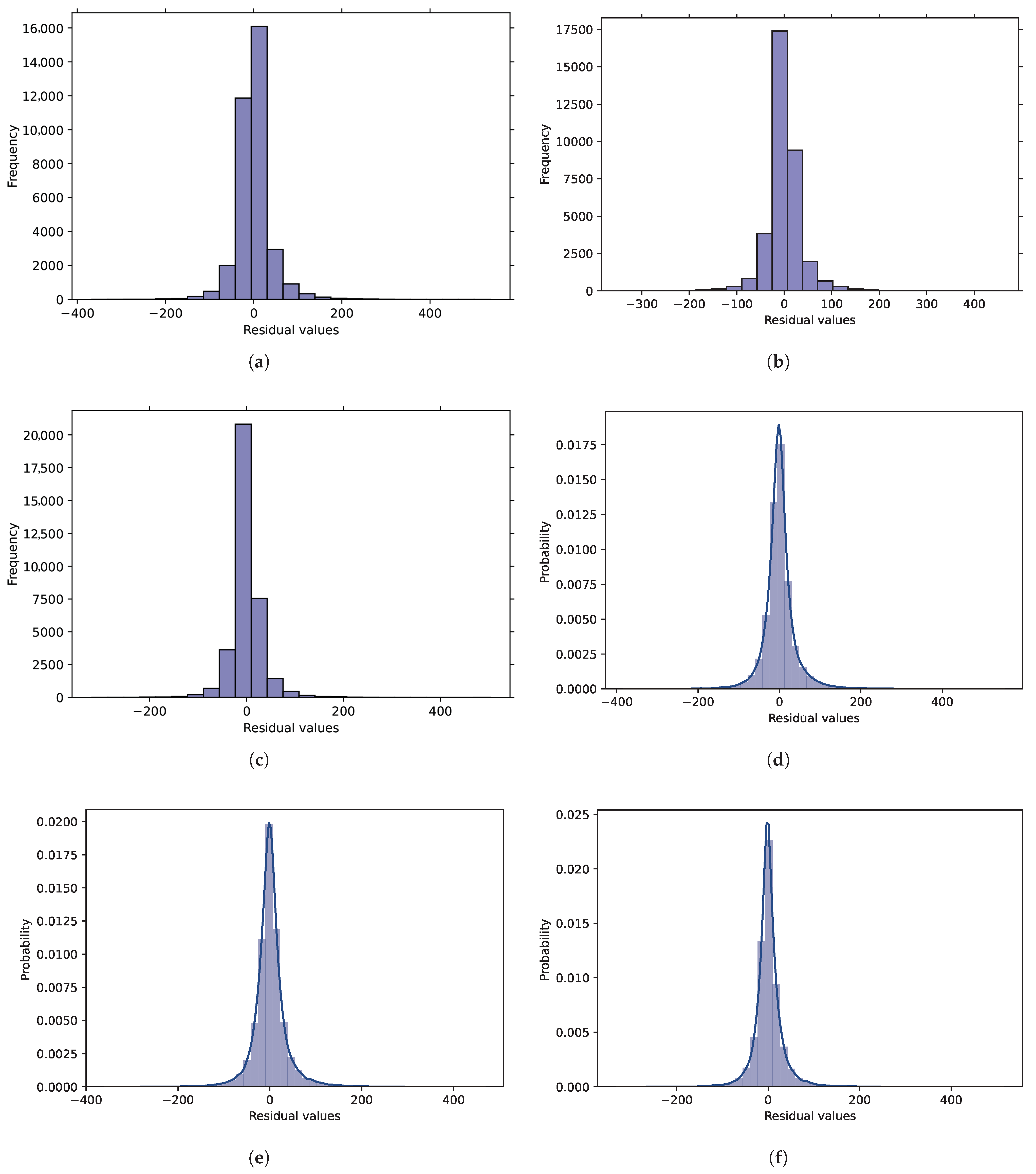
To further analyze the performance of the BFGS-URWELM, the residuals of the ELM, URWELM, and BFGS-URWELM algorithms were analyzed. Figure 4 illustrates the probability density plots and histograms of the prediction residuals of the ELM, URWELM, and BFGS-URWELM algorithms.

Figure 5a–c show the residual distribution of different algorithms. The closer the residual is to 0, the smaller the prediction error. In contrast, the residuals of the ELM algorithm were mainly concentrated near 0, but the distribution was wider, and the error was larger; the residual distribution of the URWELM algorithm was more concentrated, indicating that the prediction stability had improved, and the error had decreased; the residual distribution of the BFGS-URWELM algorithm was the most concentrated and had the highest peak, indicating that it had the highest prediction accuracy, the smallest error, and the best performance. Overall, the optimized algorithm improved both the prediction accuracy and stability. 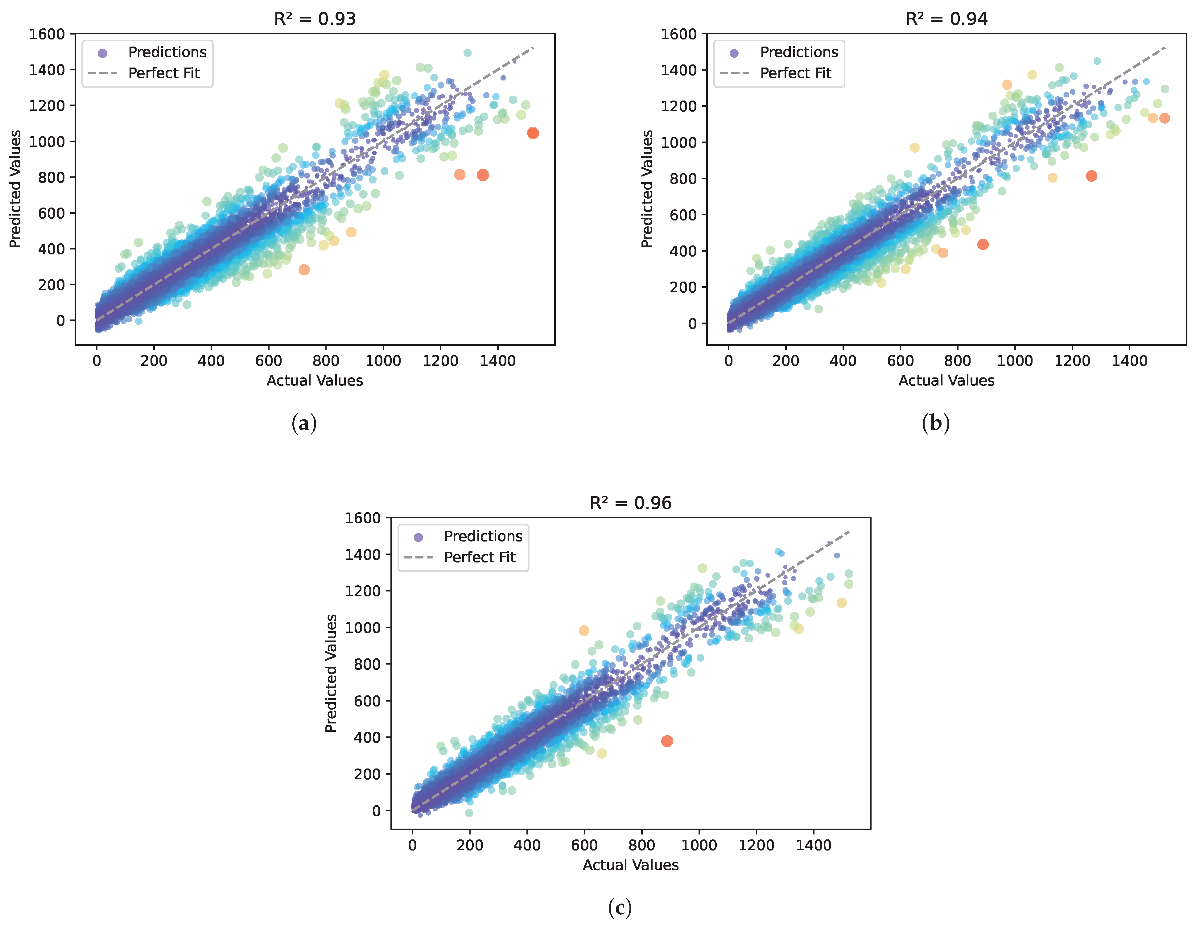Figure 4d–f reflect the residual distribution of different algorithms and fit them through smooth curves. The residual distribution of the ELM algorithm is wider, indicating that the prediction error is larger; the residual distribution of the URWELM algorithm is more concentrated than that of the ELM, with a higher peak value, indicating that this method effectively reduces the error; the residual distribution of the BFGS-URWELM algorithm is the most concentrated, with the narrowest curve and the highest peak value, indicating that it has the smallest prediction error and the best performance. The residual weighting method can effectively improve the stability of the ELM, and the BFGS optimization is further optimized, reflecting the improvement in prediction accuracy by algorithm optimization. Next, we will analyze the scatter plot predicted by the BFGS-URWELM algorithm, as shown in Figure 5.

From Figure 5, we can find that compared to the ELM algorithm ($R^2=0.93$), the URWELM algorithm ($R^2=0.94$) has a more concentrated scatter distribution, which reduces prediction error, especially in the high-value area. The further optimized BFGS-URWELM algorithm ($R^2=0.96$) performed best, with the highest degree of fit between the predicted value and the true value, the most dense scatter distribution, and the deviation in the high-value range further reduced, indicating that BFGS optimization improved the generalizability of the model. In general, the algorithm improvement increased the $R^2$ by 3.23% overall, significantly improving the accuracy and stability of the prediction.

3.3. Comparison with ELM Variants

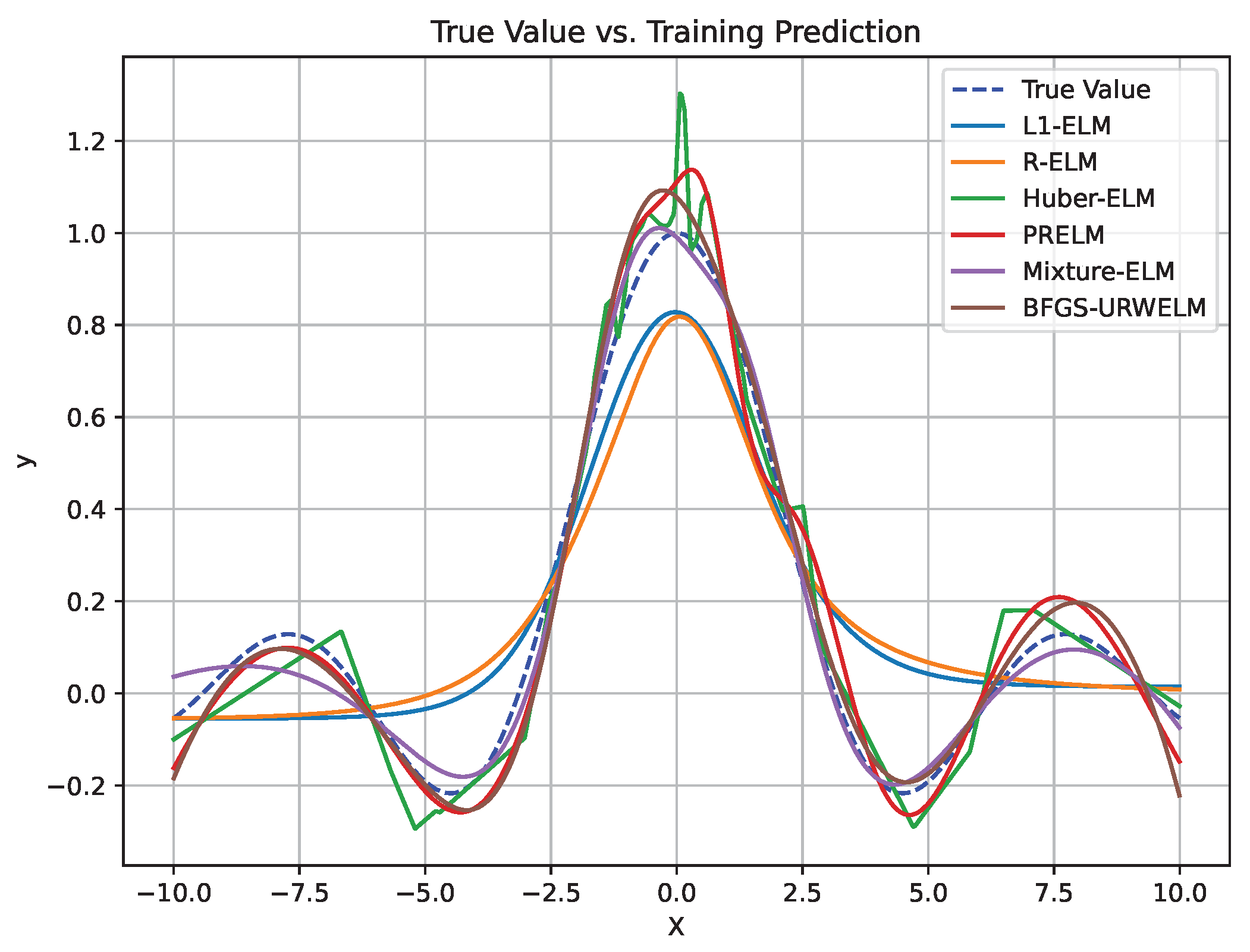
In our evaluation, we utilized the following “SinC” function:

$$y\left(x\right)=\left\{\begin{array}{cc}{\displaystyle \frac{sin\left(x\right)}{x}},\hfill & x\ne 0,\hfill \\ 1,\hfill & x=0\hfill \end{array}\right.$$

(30)

For the mixed noise scenario, the noise was generated using a combination of different distributions: 80% was drawn from the Gaussian distribution $N(0,1)$, and 20% originated from the Laplace distribution $L(0,0.1)$. To better analyze the performance of the BFGS-URWELM, it was compared with the original ELM and some variants of the ELM algorithm, such as the Lasso-ELM (LELM), Ridge-ELM (RELM), ELM with Huber loss function (Huber-ELM), PRELM [28] and mixture ELM [25]. Figure 6 shows the performance of six different algorithms on mixed noise-contaminated training data. The specific performance is shown in

Table 5. Comparison of RMSE, MAPE, and MAE by LELM, RELM, Huber-ELM, PRELM, BFGS-URWELM, and mixture ELM.

Algorithms	MAE		RMSE		MAPE
	Train	Test	Train	Test	Train	Test
LELM	$0.514\pm 0.022$	$0.184\pm 0.033$	$0.747\pm 0.021$	$0.233\pm 0.049$	$2.918\pm 2.076$	$6.475\pm 18.557$
RELM	$0.537\pm 0.014$	$0.216\pm 0.019$	$0.767\pm 0.016$	$0.283\pm 0.026$	$4.189\pm 9.360$	$8.201\pm 11.506$
Huber-ELM	$0.504\pm 0.017$	$0.163\pm 0.031$	$0.741\pm 0.018$	$0.196\pm 0.036$	$3.081\pm 2.086$	$5.208\pm 7.043$
PRELM	$0.457\pm 0.013$	$0.063\pm 0.022$	$0.711\pm 0.017$	$0.078\pm 0.025$	$3.287\pm 5.788$	$3.060\pm 3.908$
Mixture ELM	$0.369\pm 0.017$	$0.368\pm 0.017$	$0.501\pm 0.016$	$0.500\pm 0.015$	$1.960\pm 0.140$	$1.959\pm 0.144$
BFGS-URWELM	$0.355\pm 0.009$	$0.047\pm 0.010$	$0.494\pm 0.014$	$0.059\pm 0.012$	$3.560\pm 4.362$	$1.748\pm 1.735$

.

The BFGS-URWELM exhibited extremely low errors in the MAE and RMSE, with the test set showing an MAE of 0.047 and an RMSE of 0.059. This indicates excellent predictive accuracy and strong generalization capability. Although the training MAPE was relatively high at 3.560, the test MAPE was very low at 1.748, demonstrating high stability and robustness in practical applications. In contrast, the mixture ELM showed moderate performance in the MAE and RMSE, with a test MAE of 0.368 and a test RMSE of 0.500. However, it achieved superior performance in terms of its relative error, since both the training and test MAPEs were approximately 1.96. In summary, when predictive accuracy is the primary focus with emphasis on the MAE and RMSE, the BFGS-URWELM is clearly superior, while the mixture ELM excels when relative error measured by MAPE is the key consideration.

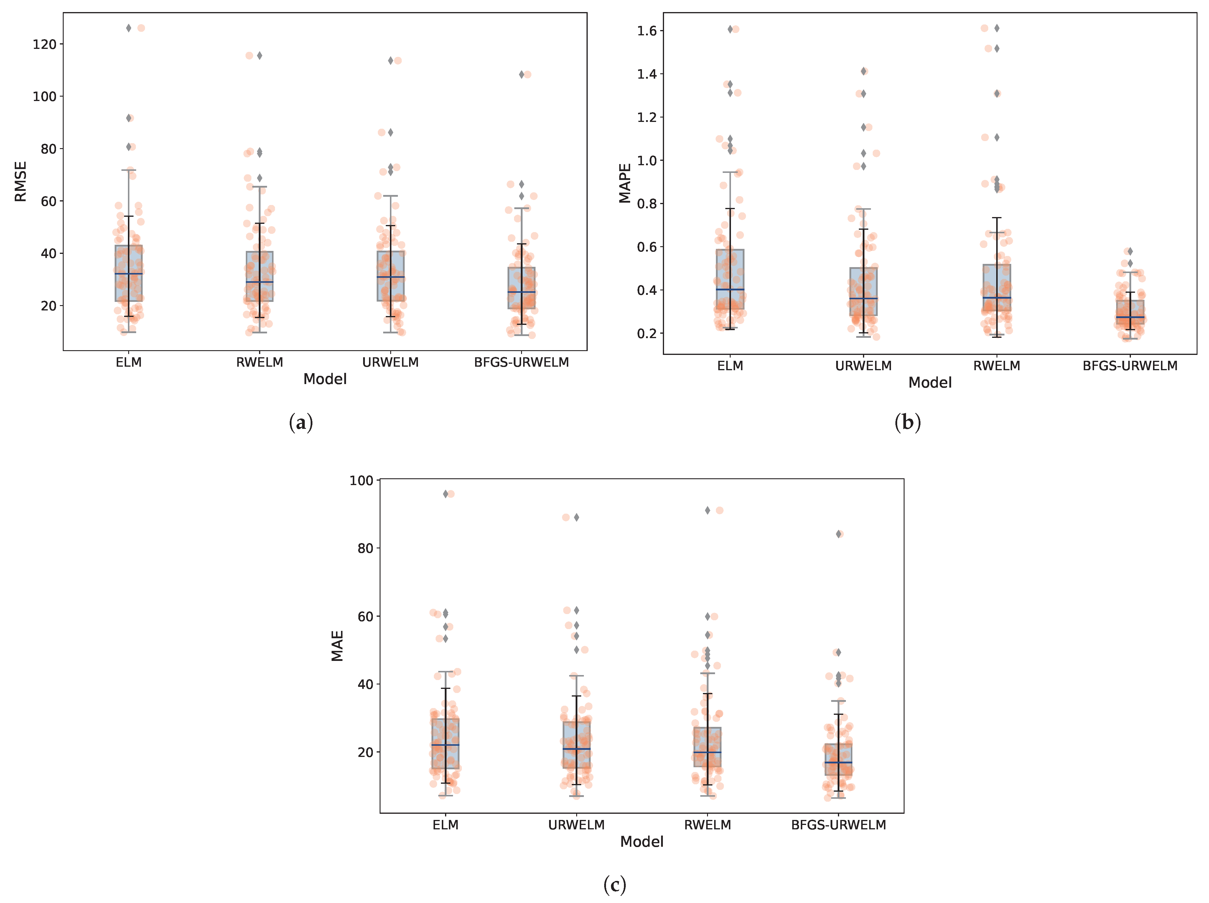
To verify the performance of the BFGS-URWELM in subway passenger flow data, it was compared with the ELM variant algorithms. The original subway station passenger flow data within the 5-min sampling period wew also summarized using a seven-step sliding window. The subway passenger flow data for 21 days were used for training, and the data for the 22nd and 23rd days were used as the test set. The performance of the ELM variants was examined in terms of the RMSE, MAPE, and MAE, as depicted in Figure 7.

Figure 7 illustrates that the BFGS-URWELM algorithm exhibited significant advantages in controlling both the overall and absolute errors, as indicated by its superior RMSE and MAE performance, even though its MAPE was marginally lower than those of the mixture ELM and Huber-ELM. The mixture ELM, on the other hand, excelled in relative error metrics (MAPE) while maintaining moderately competitive RMSE and MAE values. Similarly, the PRELM shows stable performance comparable to the BFGS-URWELM in terms of the RMSE and MAE, albeit with a slightly higher MAPE. The Huber-ELM is noteworthy for its robust handling of relative errors, likely due to its effective treatment of outliers and noise. In contrast, L1-ELM, RELM, and the original ELM consistently underperformed across all three metrics, with the ELM was particularly affected by a wider error distribution and more pronounced outliers. Overall, the integration of weighting, regularization, hybrid strategies, and advanced optimization techniques (such as BFGS and Huber loss) significantly enhanced the predictive accuracy and stability, with the BFGS-URWELM and mixture ELM offering particularly robust comprehensive performance. The performance of each algorithm is shown in

Table 6. Comparative performance metrics of ELM variants.

Different ELM	Mean RMSE	Mean MAPE	Mean MAE
ELM	35.3802	0.4621	24.7924
RELM	34.3599	0.4623	24.2403
Huber-ELM	29.2575	0.3069	20.4437
L1-ELM	34.2782	0.4590	24.2270
Mixture ELM	29.0526	0.2920	20.2370
PRELM	28.7853	0.3169	20.1645
BFGS-URWELM	28.3361	0.3071	19.7599

.

Table 6 shows that the baseline ELM model had the highest error rates with an RMSE of 35.38, an MAPE of 0.4621, and an MAE of 24.79. Simple regularization approaches in the RELM and L1-ELM yielded only marginal improvements. In contrast, the Huber-ELM significantly reduced the errors with an RMSE of 29.26, an MAPE of 0.3069, and an MAE of 20.44, while the mixture ELM and PRELM were further enhanced in terms of performance; the mixture ELM achieved the lowest MAPE at 0.2920. Notably, the BFGS-URWELM achieved the lowest RMSE at 28.34 and the lowest MAE at 19.76, indicating superior overall error control. These findings underscore the benefits of integrating advanced optimization techniques and robust loss functions to improve predictive accuracy and stability in ELM-based models.

3.4. Comparison with Other Algorithms

To assess the algorithm and demonstrate its ability to generalize, traffic flow predictions were made for 80 different subway stations. The training dataset included data from the initial 22 days of every dataset, with the 23rd and 24th days set aside for model testing. The BFGS-URWELM’s performance was measured against several popular traffic flow models like ARIMA [29], Multilayer Perceptron (MLP) [30], K-nearest neighbor (KNN) [31], decision tree (DT) [32], and SVM [33]. Ensemble learning models included the XGBoost [34], Catboost [35], LGB [36], and random forest algorithm (RF) [37]. The Python 3.7 was used. The scikit-learn [38] library was used for machine learning algorithms to implement the baseline model, and the parameters used the recommended default parameters. In addition, deep learning-based models were incorporated into the comparison to better reflect the current state of the art. These include Stacked Autoencoders (SAEs) [39], long short-term memory networks (LSTMs) [40], Gated Recurrent Units (GRUs) [41], and the Transformer [42], all of which have demonstrated strong performance in time series forecasting and sequence modeling tasks. 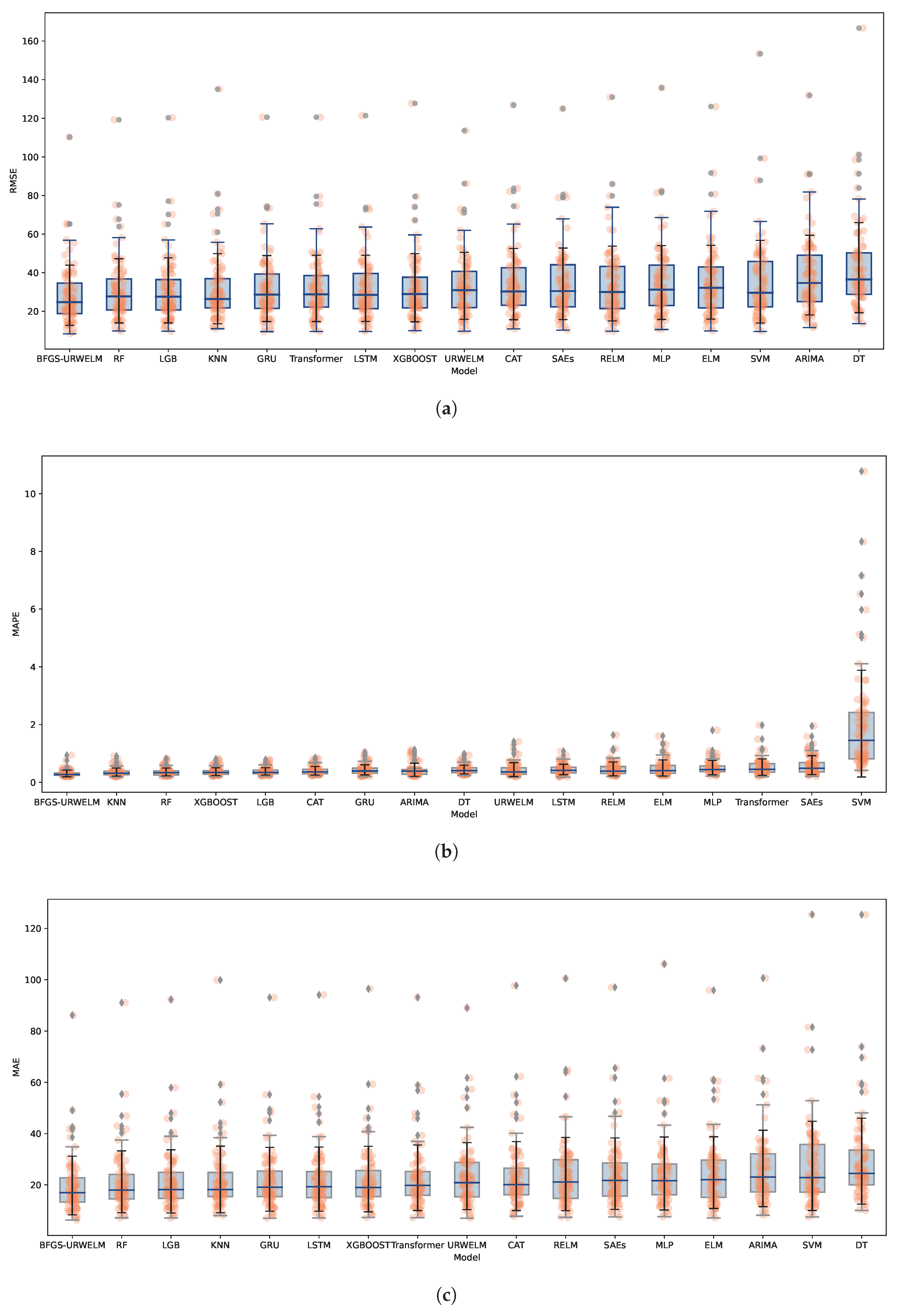The performance of the BFGS-URWELM, along with MLP, DT, XGBoost, SVM, RF, etc., was examined in terms of the RMSE, MAPE, and MAE results, as depicted in Figure 8.

As shown in Figure 8, BFGS-URWELM achieved the best performance across all three evaluation metrics—RMSE, MAPE, and MAE—demonstrating its superior prediction accuracy and strong stability. Compared to its variants, the BFGS-URWELM significantly outperformed the standard ELM, RELM, and URWELM models, highlighting the effectiveness of the BFGS optimization in enhancing the model’s generalization ability. Models such as DT, SVM, and ARIMA exhibited the highest errors, indicating that they struggled to capture complex temporal patterns in the dataset. The BFGS-URWELM also outperformed traditional ensemble methods, including RF, LGB, and XGBoost, as well as deep learning approaches like LSTM, GRU, SAEs, and Transformer; more details are shown in

Table 7. The performance of different algorithms under the evaluation index.

Algorithm	Mean RMSE	Mean MAPE	Mean MAE
SVM	35.3491	2.0345	27.3958
KNN	31.7124	0.3540	22.1114
DT	42.6030	0.4411	29.2491
RF	30.6160	0.3599	21.1964
XGBOOST	32.1976	0.3682	22.2800
MLP	34.9093	0.5092	24.4200
LGB	30.8594	0.3780	21.3504
CAT	34.0626	0.4013	23.4539
ARIMA	38.7573	0.4347	26.4184
BFGS-URWELM	28.3361	0.3071	19.7599
ELM	35.3802	0.4621	24.7924
RELM	34.3599	0.4623	24.2403
URWELM	32.5040	0.4563	23.1073
LSTM	31.8898	0.4446	22.2544
GRU	31.7643	0.4310	22.2044
SAEs	34.2082	0.5978	24.3866
Transformer	31.8642	0.5247	22.7977

.

Further performance comparisons are detailed in Table 7, which presents the average RMSE, MAPE, and MAE across all evaluated algorithms. Among the 17 tested models, the BFGS-URWELM consistently achieved the lowest errors on all three metrics, with a mean RMSE of 28.3361, a mean MAPE of 0.3071, and a mean MAE of 19.7599. The most significant relative improvements appear when compared to SAEs and decision trees, showing an 84.91% reduction in mean MAPE compared to SAEs, a 33.49% decrease in mean RMSE compared to decision trees, and a 32.44% decrease in mean MAE compared to decision trees. Even against strong contenders such as LightGBM, GRU, and Transformer, the BFGS-URWELM maintained a clear advantage. The smallest observed improvements still reflect meaningful gains, including a 7.45% reduction in the RMSE over LightGBM, a 13.25% improvement in the MAPE over random forest, and a 6.78% reduction in the MAE over random forest. On average across all models, the BFGS-URWELM delivered a 17.03% improvement in the RMSE, a 30.91% improvement in the MAPE, and a 17.48% improvement in the MAE, with the MAPE showing the most substantial progress. These results highlight the BFGS-URWELM’s exceptional ability to reduce relative error while also consistently enhancing absolute accuracy, reinforcing its robustness and effectiveness in traffic flow prediction across a wide range of subway stations.

In order to evaluate the performance significance of the proposed algorithm in terms of the RMSE, MAPE, and MAE, the Wilcoxon signed-rank test was used to perform statistical tests with the comparison algorithm. The test results show that the proposed algorithm was significantly better than the comparison algorithm in all indicators (p < 0.05), indicating that the proposed method has better prediction ability and generalization performance. The specific performance is shown in

Table 8. Wilcoxon, p-value and sig for each model under the RMSE, MAPE, and MAE metrics.

Model	RMSE/MAPE/MAE
	Wilcoxon	p-Value	Sig
ARIMA	0.0/295.0/0.0	$7.8495\times {10}^{-15}$/$2.0832\times {10}^{-10}$/$7.8495\times {10}^{-15}$	Yes/Yes/Yes
DT	1.0/153.0/0.0	$8.1524\times {10}^{-15}$/$1.9762\times {10}^{-12}$/$7.8495\times {10}^{-15}$	Yes/Yes/Yes
MLP	44.0/8.0/0.0	$4.0634\times {10}^{-14}$/$1.0619\times {10}^{-14}$/$7.8495\times {10}^{-15}$	Yes/Yes/Yes
SAEs	44.0/32.0/0.0	$4.0634\times {10}^{-14}$/$2.6064\times {10}^{-14}$/$7.8495\times {10}^{-15}$	Yes/Yes/Yes
SVM	49.0/0.0/0.0	$4.8846\times {10}^{-14}$/$7.8495\times {10}^{-15}$/$7.8495\times {10}^{-15}$	Yes/Yes/Yes
CAT	52.0/198.0/1.0	$5.4534\times {10}^{-14}$/$9.0838\times {10}^{-12}$/$8.1524\times {10}^{-15}$	Yes/Yes/Yes
ELM	56.0/218.0/0.0	$6.3143\times {10}^{-14}$/$1.7632\times {10}^{-11}$/$7.8495\times {10}^{-15}$	Yes/Yes/Yes
LSTM	59.0/121.0/3.0	$7.0463\times {10}^{-14}$/$6.4965\times {10}^{-13}$/$8.7929\times {10}^{-15}$	Yes/Yes/Yes
GRU	62.0/225.0/3.0	$7.8616\times {10}^{-14}$/$2.2192\times {10}^{-11}$/$8.7929\times {10}^{-15}$	Yes/Yes/Yes
RELM	71.0/200.0/0.0	$1.0905\times {10}^{-13}$/$9.7106\times {10}^{-12}$/$7.8495\times {10}^{-15}$	Yes/Yes/Yes
URWELM	74.0/268.0/8.0	$1.2157\times {10}^{-13}$/$8.8979\times {10}^{-11}$/$1.0619\times {10}^{-14}$	Yes/Yes/Yes
Transformer	99.0/137.0/42.0	$2.9832\times {10}^{-13}$/$1.1363\times {10}^{-12}$/$3.7744\times {10}^{-14}$	Yes/Yes/Yes
XGBOOST	110.0/402.0/30.0	$4.4083\times {10}^{-13}$/$5.1616\times {10}^{-09}$/$2.4197\times {10}^{-14}$	Yes/Yes/Yes
LGB	152.0/243.0/158.0	$1.9093\times {10}^{-12}$/$3.9890\times {10}^{-11}$/$2.3465\times {10}^{-12}$	Yes/Yes/Yes
RF	221.0/483.0/225.0	$1.9462\times {10}^{-11}$/$4.9422\times {10}^{-08}$/$2.2192\times {10}^{-11}$	Yes/Yes/Yes
KNN	336.0/561.0/202.0	$7.3468\times {10}^{-10}$/$3.7889\times {10}^{-07}$/$1.0380\times {10}^{-11}$	Yes/Yes/Yes

.

4. Conclusions

An improved extreme learning machine algorithm (BFGS-URWELM) has been proposed, which integrates uniform residual weighting with the BFGS quasi-Newton optimization method to enhance prediction accuracy and robustness. Through comprehensive experimental evaluation across 80 subway stations, we demonstrated the superiority of the BFGS-URWELM over traditional machine learning algorithms, ensemble learning methods, and various ELM variants. The experimental findings indicate that the BFGS-URWELM substantially enhanced all three performance metrics: the RMSE, MAPE, and MAE. An in-depth examination of the residual distributions reveals that the BFGS-URWELM effectively concentrated the prediction residuals around zero, thereby reducing variance and boosting generalization ability. The scatter plots show a higher coefficient of determination ($R^2=0.96$) compared to the ELM ($R^2=0.93$) and URWELM ($R^2=0.94$), highlighting the improved predictive consistency and accuracy of the proposed approach.

In addition to the directions discussed above, future research will focus on extending the BFGS-URWELM to handle non-Gaussian noise environments. Recognizing that real-world data often exhibit noise characteristics that deviate from the Gaussian assumption—such as heavy-tailed or skewed distributions—we plan to investigate modifications to the weighting scheme and update rules that can robustly accommodate these alternative noise models. Such adaptations are expected to further enhance the model’s generalization ability and predictive accuracy under more diverse and challenging conditions. Recognizing the increasing importance of data security and privacy in many modern applications, our work also considers the trade-offs between implementing enhanced security measures and the associated computing overhead. In security-critical environments, deploying encryption or privacy-preserving techniques (such as homomorphic encryption or differential privacy) can safeguard sensitive data. However, these security measures introduce additional computational demands, which may affect real-time processing capabilities. Therefore, while the BFGS-URWELM achieved superior predictive performance, its deployment in contexts that require stringent security protocols must balance these enhancements against potential performance penalties.

The integration of the BFGS quasi-Newton optimization, while boosting accuracy, increases computational load, which can be a critical factor in real-time or large-scale applications. The current implementation does not incorporate intrinsic security measures. For applications handling sensitive or private information, additional security layers must be integrated, further impacting computational efficiency. To address these challenges and extend the capabilities of the BFGS-URWELM, future research should consider the following targeted directions. Investigate the incorporation of lightweight encryption or privacy-preserving techniques that offer robust security without significantly compromising computational efficiency. Explore integrating federated learning approaches to ensure data privacy during the training phase, thereby mitigating risks associated with centralized data storage. Examine the resilience of BFGS-URWELM against adversarial attacks and implement countermeasures, such as adversarial training, to enhance its robustness.

Overall, the integration of uniform residual weighting and BFGS optimization effectively addresses the limitations of the traditional ELM, leading to superior predictive performance and robustness. With focused enhancements to manage security-related computing overhead and a clearer understanding of its limits, the BFGS-URWELM shows promise as a viable approach for traffic flow prediction and other time series forecasting tasks where both accuracy and data integrity are essential.