Empirical Analysis of Hierarchical Pathfinding in Lifelong Multi-Agent Pathfinding with Turns ^†

Abstract

Lifelong multi-agent pathfinding has two interrelated aspects: one is to find conflict-free paths for the agents, and the other is to resolve the conflicts among the agents in the best possible way. We focus on the first aspect by investigating three hierarchical pathfinding approaches, while we apply the same conflict resolution method. We formally present the three pathfinding options: map reduction using fixed waypoints, map reduction using dynamic waypoints, and the classic grid region-based approach. We point out the problem of emerging conflicts in lifelong multi-agent pathfinding with turns. We describe how we evaluate the proposed solutions to example scenarios from the League of Robot Runners competition, and we formulate the goals of the empirical analysis. Based on the experimental results, we point out the need to find the sweet spot between response time and throughput.

1. Introduction

In many multi-agent systems, the agents have to solve the problem of navigating in the environment without colliding with other agents or obstacles. This is needed in many applications including traffic control, video game character control, warehouse automation, and many more. A well-known abstract model for this problem is Multi-Agent Pathfinding (MAPF) [1].

Finding the optimal and complete solution for the MAPF problem is NP-hard [2] and cannot be applied at the scale of practical applications. There are search algorithms for solving MAPF in practice, but they may either have limited scalability, or may generate an expensive solution, or may fail to find a suitable path in the case of difficult graphs and problems [3]. Big e-commerce companies are interested in MAPF research [4]. Game developers tackle the pathfinding complexity by dividing the map into polygons1 to create a hierarchical abstract level map.

Lifelong multi-agent pathfinding has two interrelated aspects: one is to find conflict-free paths for the agents, and the other is to resolve the direct and the emerging conflicts among the agents in the best possible way. We focus on the first aspect by investigating three hierarchical pathfinding approaches, while we apply the same conflict resolution method. The three pathfinding options are as follows: map reduction using fixed waypoints2, map reduction using dynamic waypoints, and the classic grid region-based approach. The initial versions of the first two waypoint approaches are described in [5] and the original version of the grid region based approach is described in [6].

We target pathfinding because, if the pathfinding is faster, there is more time for local repair heuristics to produce better solutions like in [7]. Faster pathfinding methods instead of usual graph search algorithms are also essential if the map is large and there are many agents. The maps discussed in this paper, or larger maps, may benefit from hierarchical pathfinding. Usual pathfinding algorithms work well on smaller maps, and hierarchical pathfinding may be less effective on them.

We use an extended version of the well-known Cooperative A* search algorithm [8] to resolve the direct conflicts among the paths of the agents. As an extension, we use safe interval path planning [9] instead of the classic A* algorithm. We use the reservation table of the Cooperative A* search algorithm to detect emerging conflicts among the agents, and we avoid possible collisions with turns.

We evaluate the three hierarchical pathfinding methods on the example scenarios from the League of Robot Runners3 competition. The scenarios include three different types of maps and several agent team sizes. These maps are fixed during the experiment, like in usual MAPF test scenarios.

Most studies on hierarchical pathfinding [10,11] either focus on the one-shot MAPF problem and do not take into account the lifelong aspects nor turn movements, or they focus on the parallel computing aspects [12]. The original grid region-based approach contains a path-smoothing algorithm, but it cannot be applied directly when the space–time search of [8] is used. In this context, path smoothing is related to the movements on a grid map environment, where the robots move in time steps, and we do not have to go into the details of real-world robot movements which is discussed for example in [13]. If the windowed search is used in the case of lifelong MAPF with turns, then emerging conflicts are generated by the space–time search.

Our contributions are the formal description of the map-reduction methods of [5], the modification of the path-smoothing method of the classic grid region based approach [6] for lifelong multi-agent space–time search with turns, and the empirical comparison of these approaches. These contributions may be useful when designers select the right pathfinding methods for different types of maps and scenarios.

In Section 2, we describe the problem of this study. In Section 3, we formally present the proposed solutions to be used in the empirical analysis. In Section 4, we describe how we evaluate the proposed solutions, and we formulate the goals of the empirical analysis. In Section 5, we present the results of the experiments. In Section 6, we evaluate the results. Finally, we conclude the empirical analysis in Section 7.

2. Problem Statement

2.1. MAPF Version

There are different versions of the MAPF problem. In the classic MAPF verion, there are m agents $A=\{a_1,a_2,\dots a_m\}$ which move on a grid map. The map is represented by a graph $G=(V,E)$ where V are the vertices and E are the edges. Agents have their start and goal vertices: $s_i\in V$ and $g_i\in V$. The start vertices are different for every agent, and the goal vertices are usually different too. Let $l_i\left(t\right)\in V$ denote the location of agent $a_i$ in discrete timestep t. Agent $a_i$ starts in its initial location $l_i\left(0\right)=s_i$. At each step, an agent can move to an adjacent vertex or wait at its current vertex, that is, $l_i(t+1)=l_i\left(t\right)$ or $(l_i\left(t\right);l_i(t+1))\in E$. The agents have to avoid collisions when two agents move to the same vertex or traverse the same edge at the same step. Formally: two agents cannot be in the same location in the same timestep, that is, $\forall a_i,a_j\in A:a_i\ne a_j\Rightarrow \forall t:l_i\left(t\right)\ne l_j\left(t\right)$, and two agents cannot move along the same edge in opposite directions in the same timestep, that is, $\forall a_i,a_j\in A:a_i\ne a_j\Rightarrow \forall t:l_i\left(t\right)\ne l_j(t+1)\vee l_i(t+1)\ne l_j\left(t\right)$. The target is to find collision-free paths for all agents to their goals. The agents are expected to optimize their paths, like minimizing the total number of moves or minimizing the make-span.

In the lifelong (LMAPF) version of the above MAPF, the agents are constantly assigned new goals. The optimization criterion is to maximize throughput, measured by the number of goals reached by all agents during a given number of steps.

In the MAPF with Turns (MAPF-T) version of the above MAPF, the state of an agent is determined by its location $v\in V$ plus an orientation $o\in \{East, South, West, North\}$. At each step, an agent can move forward to an adjacent vertex in accordance with its orientation, rotate 90 degrees clockwise or counterclockwise, or wait at its current vertex.

The MAPF version of the League of Robot Runners competition is lifelong MAPF with Turns (LMAPF-T) which is a combination of LMAPF and MAPF-T. The agents are constantly assigned new goals, and their movement rules are that of MAPF-T. The LMAPF-T problem can be regarded as an abstract model of the Amazon warehouse [4]. Our investigations focus on this LMAPF-T problem.

2.2. Pathfinding

Because the optimal and complete MAPF algorithms, like Conflict-Based Search (CBS) [14], are computationally intractable, several algorithms have been developed without guarantee on optimality and/or completeness. Bounded suboptimal algorithms, like Enhanced CBS (ECBS) [15], guarantee solutions within a given bound, but do not scale to large warehouses and their real-time requirements. Prioritized algorithms, like [16], decouple the search algorithm into a series of single agent searches to increase speed, but they are neither complete nor optimal. Computation time can be reduced if conflicts among the individual agent searches are resolved only within a limited distance ahead, and the conflict resolutions are updated as agents progress, like [17]. The conflict resolution part can be made faster with the large neighbourhood technique [18] known for combinatorial optimisation. The Priority Inheritance with Backtracking (PIBT) algorithm [19] combines the shortest path planning and reservation with prioritization and backtracking to avoid deadlocks, and achieves very fast operation even in the case of large number of agents, but loses on solution quality.

Many of the above algorithms use the concepts of the Cooperative A* (CA*) search algorithm [8], where pathfinding is decoupled into a series of single-agent searches. The individual searches are performed in three-dimensional space–time (two spatial dimensions and one time dimension). After each agent’s route is calculated, the future locations along the route are recorded into a reservation table, and these entries in the reservation table are considered impassable during searches by subsequent agents. The reservation table is in fact a form of intention awareness which is used in other multi-agent route planning applications as well, like vehicle routing [20]. This intention awareness has some proven problems [21] caused by the fact that agents cannot take into account intentions submitted after their own plan is created, and, in some cases, the traffic in vehicle routing may be worse off by exploiting intention awareness than without exploiting intention awareness. This three-dimensional search is often called space–time search.

In our empirical analysis, we use safe interval path-planning (SIPP) [9] which is an enhanced form of the Cooperative A* algorithm. SIPP has many advantages over CA*. One advantage is that the search space is reduced, because consecutive future time steps at the same location without entries in the reservation table are merged into a single state. Another advantage is that SIPP treats a location differently before and after the passing of an agent through that location. This allows an agent to step aside and lets another agent pass by and step back to the same location to continue on its path. In A*, this is not possible because in the A* algorithm stepping back to the same location is a longer path to the same position, therefore it is excluded. We sometimes call the SIPP algorithm state-time search.

The core of most of the above algorithms is the pathfinding for a single agent. The different versions of the A* algorithm need more and more time as the size of the map grows. Hierarchical pathfinding [6] can mitigate this problem by creating a higher-level abstraction of the search space. Because the abstraction level map is smaller than the low-level map, the search on this higher-level map is faster. The skeleton of the path, created on the higher level map, is then filled with shorter-distance searches on the lower level. The resulting path is then smoothed to get a near-optimal path. However, the known smoothing algorithm works for a single agent, and in a CA* or SIPP context, another kind of smoothing is needed. We present such a smoothing approach in the next section and empirically analyse its working in LMAPF-T problems.

There is another issue when hierarchical pathfinding is used in combination with the CA* and SIPP algorithms. The reservations of these algorithms originate from the paths of the low-level search, while skeleton of the path is fixed at the high level, which may result in congestions in certain parts of the high-level path. It might be possible that it would be better to search for an alternative high-level path instead of avoiding the reservations at the low level. Our empirical analysis touches on this congestion issue as well.

2.3. Emerging Conflicts in LMAPF-T

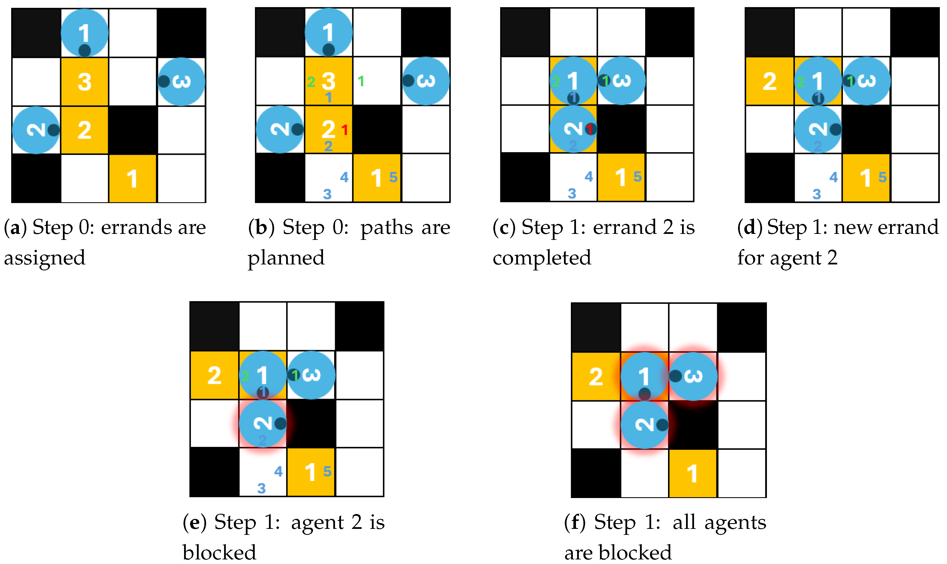
In the one shot MAPF and MAPF-T problems, the reservation tables of the CA* and the SIPP algorithms guarantee that the paths are conflict-free paths. Unfortunately, in the LMPAF-T problem, this is not enough, and a new type of conflict may emerge because of the continuous errand assignments and the turn movements. This emerging conflict is illustrated in Figure 1.

There are three agents (blue circles on the figure and their orientation is marked with dark blue dots) with their corresponding target locations (yellow cells) on the map of Figure 1a. The priorities of the agents are the same as their numberings. The agents individually plan their path, and record their reservation in the reservation table, as shown in Figure 1b. The smaller-sized numbers show the reservation for a given cell in a given time step. The position of the number in the cell indicates the orientation of the agent in the cell. The blue numbers are for agent 1, the red numbers are for agent 2, and the green ones are for agent 3. The reservations are only until the agent reaches its target location because, after that, the agent will receive a new target location which is not known at the time of the planning. Agent 2 is happy to plan to move into its goal cell in time step 1, because there is no reservation for that time step. In time step 1, the agents move as planned (Figure 1c) and a new target location is assigned to agent 2 (Figure 1d). Agent 2 is unable to plan its path to the new target location because every path would need a turn movement in the same location, and that location is already reserved by agent 1 for time step 2 (Figure 1e). Agent 1 is blocked, and this escalates to agent 1 and 3 as well (Figure 1f).

This emerging conflict is specific to LMAPF-T; therefore conflict-checking needs to be performed in each time step for agents who would advance to another cell. We can detect the conflict using the reservation table and the location of the agents. We use a simple technique to resolve the conflict. The agent who would have entered into a conflict—instead of moving forward—stays in place and randomly turns in one direction or the other. Since the turn also takes time, it is hoped that there will be a time shift between the lengths of the paths of the agents in conflict, which will be able to direct the agents towards new paths. Because of the possibility of the above mentioned escalation, we have to re-examine whether a new conflict would arise with another agent. Conflict detections and corrections must be repeated until there is no conflict with any of the agents. This conflict resolution can prevent collisions, but does not solve the problem optimally, and there may be cases where the agents come to a standstill in a narrow part of the map. There are better conflict resolution methods (see above in this section), but this simple method is enough for our experimental analysis because we want to evaluate the robustness of the different hierarchical search methods against this emerging conflict. One could even say that the simple conflict resolution method is better for this analysis because it enlarges any weaknesses of the hierarchical search.

Because hierarchical search and the rolling horizon approach [17] cut the pathfinding into smaller pieces, the emerging conflicts in the LMAPF-T problem may intensify. Our empirical analysis addresses this issue as well.

3. Hierarchical Search Methods in the Analysis

3.1. Map Reduction to Fixed or Dynamic Waypoints

We have created a novel approach for hierarchical pathfinding. An earlier version of this approach is described informally in [5]. The approach uses waypoints which are created with the help of map reduction. The intuitive outline is the following. First we reduce the free part of the map by leaving out the free cells at the edge of the free area until only a single lane remains in the middle of the free area. Then we create waypoints on these lanes at specific distances. The waypoints may be fixed on the map, and then the high-level path is created from the set of these fixed waypoints for all agents. In another version, the waypoints are created dynamically for each agent, and then the agents may create their high-level path from different set of waypoints. The pathfinding on the waypoints works very fast, and the pathfinding from one waypoint to another one is done with the usual algorithms, which is also fast because the distances are not long.

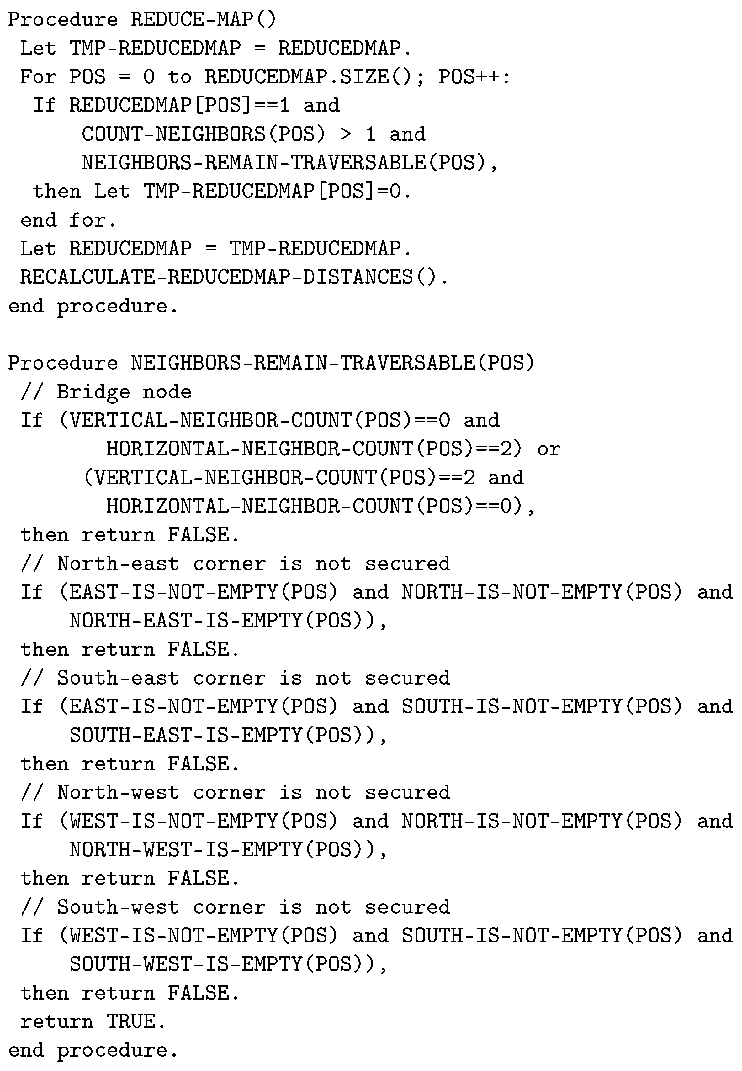
The map reduction process preliminarily initializes the reduced map by assigning to each free cell its distance from the nearest wall. This is straightforward, and it is not described here in details. Then we execute map reduction cycles. The map reduction procedure and the procedure to check traversability are shown in Figure 2. In each reduction cycle, we “delete” the free cells for which the value of the distance is 1, and “deleting” the cell does not disconnect its neighbours, thereby preserving the connectivity on the map. These “deleted” cells will still be represented as free cells, but from now on we regard them as walls when we calculate distance from walls. Then, we recalculate the distances from the walls on the reduced map using the same straightforward algorithm as in the initialization. We repeat this cycle until the graph can no longer be reduced. This gives us a skeleton of the original map with lanes in the middle of the free areas. 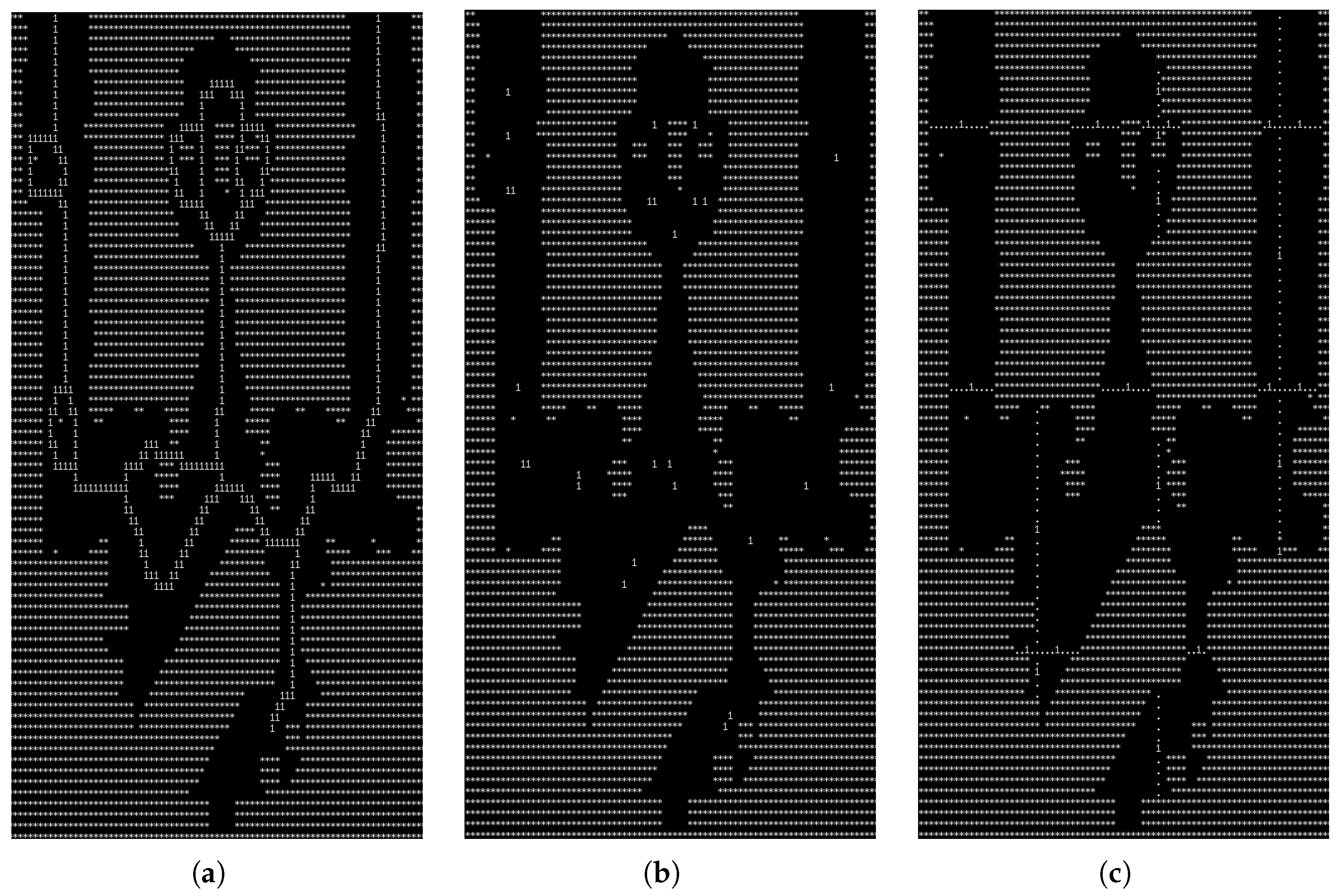Figure 3a shows the result on a part of the game map.

The lanes are used in two different ways to produce either dynamic waypoints or fixed waypoints.

Dynamic waypoints are created for each agent when the agent plans its path. The pathfinding works on the lanes using the A* algorithm. The starting location of the search is the location on the lanes closest to the agent. The target location of the search is the location on the lanes closest to the target location of the agent. When the path is found, every Nth positions along the path are kept as waypoints. If parameter N is small, then we get dense waypoints; if N is bigger, then we get sparse waypoints. These dynamic waypoints depend on the starting position; therefore the waypoints may be different for different agents along the lanes, which might be useful to avoid congestions around waypoints.

For fixed waypoints, a waypoint map is created from the lanes using the algorithm of Figure 4. The waypoint map only contains the waypoints and the links from each waypoint to its neighbouring waypoints together with the distances to the neighbours. The waypoint map is created before the actual LMAPF-T pathfinding starts; therefore all the agents use the same set of waypoints. The algorithm of Figure 4 keeps the crossing positions of the lanes, and removes other positions if the distance between the neighbours of the given position is shorter than a given parameter $N=MAXDISTANCE$. With the removal of a position, the links between its neighbours are updated with the proper distances. If a position in a corner is to be removed, the distance between its neighbours is increased by 1 to take into account a turn movement. Figure 3b shows the result of waypoint creation on a part of the game map.

Once we have either the reduced map with the lanes or the waypoint map, the pathfinding is divided into two parts.

In the first part, we search on the reduced map with lanes (in the case of dynamic waypoints) or on the waypoint map (in the case of fixed waypoints) for the position that is closest to the agent’s location, then we do the same for the target location, and these will be the starting and ending waypoints. Then, in the case of dynamic waypoints, we create the waypoints along the lanes between the starting and ending waypoints as described above, or in the case of fixed waypoints, we search on the waypoint map for a waypoint path between the start and end waypoints using the A* algorithm. In both cases, we get a waypoint path.

In the second part, the agent plans a path from its position to the proximity of the next waypoint using the SIPP algorithm on the original map and avoiding conflicts with other agents. Once the agent has found the path, it only reserves the path up to the given proximity to its target waypoint, and as soon as the agent is close enough to the waypoint (before reaching the proximity target), it plans a new path to the next waypoint. This is needed so that several agents can find the best possible route to the same waypoint and to avoid congestion. We call this technique waypoint proximity path planning. After the agent completes the path to the proximity of its current target waypoint, it discards it and plans a path to the proximity of the next waypoint again. It repeats this until it reaches the proximity of its final waypoint. Having reached the final waypoint, the agent plans a path with the SIPP algorithm to its target location. The agent not only approaches the target location cell, but also gets there exactly.

With this solution, we split the agent’s pathfinding problem into several simpler problems, where the algorithm is able to find a path very quickly, even on the largest maps. If dynamic waypoints are used, then we denote the pathfinding DynWP pathfinding, if fixed waypoints are used, then we denote the pathfinding FixWP pathfinding.

3.2. Classical Hierarchical Search: Grid Waypoints

The classical hierarchical pathfinding (HPA*) [6] creates a topological abstraction of the map, and then this map abstraction is used to build an abstract graph for hierarchical search. The representation of the abstract graph is basically the same as the waypoint map in the previous Section 3.1, the difference between the two approaches is how the waypoint locations are determined. The topological abstraction covers the map with a set of disjunct rectangular blocks. This abstraction is topology independent. For each border line between two adjacent blocks, the HPA* approach identifies a set of entrances connecting them. An entrance is a maximal obstacle-free segment along the common border of two adjacent blocks. For each entrance, the HPA* approach defines a transition in the middle of the entrance. These transitions are the waypoints where a path may lead from one block to a neighbouring block. Then the pairwise distances inside a block between the transition points at the border of the block are computed, and the transition points are linked to each other together with these distance values. This way a waypoint map is created, and the waypoint map is similar to the waypoint map in the previous Section 3.1, with the difference that in HPA* the waypoints are always on the border of the abstract level rectangular blocks. Figure 3c shows the result of this waypoint creation on a part of the game map.

Once the waypoint map is created, the pathfinding is is done in two parts, like in the previous Section 3.1. In the first part, we search a path from the starting position to the border of the block, then we search a path on the waypoint map to the border of the block of the goal position, and then from the border of that block to the goal position. This way we get a waypoint path. In the second part, the detailed path from the starting position to the goal position is created by filling in the gaps between the waypoints with usual A* search on the original map.

The detailed low-level path is optimal in the abstract graph but not necessarily in the initial problem graph. To improve the solution quality, the original HPA* approach performs a postprocessing for path smoothing. The path smoothing of the HPA* approach starts from one end of the solution. Then for each node in the solution, it checks whether a subsequent node in the path can be reached in a straight line. If this is the case, then the linear path between the two nodes replaces the initial sub-optimal sequence between these nodes.

This path smoothing of the classic HPA* approach cannot be used directly in the LMAPF-T problem if we use the SIPP algorithm because we have to take into account the reservations of other agents as well. In order to be able to use the SIPP algorithm, we apply the same waypoint proximity path planning technique as in the previous Section 3.1. The agents only plan and reserve the path up to a given proximity to their next target waypoint, and as soon as the agent is close enough to the waypoint, it plans a new path to the next waypoint. Having reached the final waypoint, the agent plans a path with the SIPP algorithm to its target location.

We denote this hierarchical pathfinding modified with the waypoint proximity path planning technique GridWP pathfinding.

3.3. Full Pathfinding Versus Windowed Pathfinding

The above hierarchical pathfinding algorithms decompose the long distance pathfinding process into several short distance pathfinding processes, and the long distance path is created by concatenating the short distance paths. There is the question, whether it is better to plan and reserve the full path already at the beginning of the journey of the agent, or it is better to plan and reserve the path always only for the next window to the next waypoint. This question may be critical in the LMAPF-T problem.

The advantage of the windowed pathfinding is that the response time might be shorter because only short distance pathfinding and reservation happens in each planning step. The disadvantage of the windowed pathfinding is that the reservations are only for a short distance, and the emerging conflict described in Section 2.3 might happen at the end of every window. The more emerging conflicts, the more time might be needed to resolve them, or even more chance for congestions if the conflict needs more time to solve. Both conflict resolution and congestion might increase the pathfinding time, and the response time of the planner might suffer this.

The advantage of the full pathfinding is that emerging conflict might happen only once at the end of the planned path. The fewer emerging conflicts, the less time might be needed to resolve them, or there may even be less chance of congestions. The disadvantage of the full pathfinding is that long pathfinding and reservation needs to be done, and the response time of the planner may be long.

We empirically compare the full and the windowed pathfinding.

4. Experimental Setup

We want to empirically analyse the hierarchical pathfinding methods of the above Section 3 in the LMAPF-T problem. The analysis is carried out based on the example scenarios4 of the 2023 League of Robot Runners competition.

Only the large map scenarios will be used in the tests because, on smaller maps, there is no need for hierarchical pathfinding. We do not carry out tests on the sortation centre map because it is very similar to the warehouse map, and previous experiences have shown that the test results are also very similar. The maps of the example scenarios in the tests are illustrated in Figure 5.

Each map has a specific style. The warehouse map has a grid style with many possible alternative high-level paths in the form of parallel corridors, but no alternatives at the low-level inside the corridor. The city map has a random style with still several possible alternative high-level paths, and also several alternatives at the low level in the large free areas. The game map has very few alternatives at the high level. The agents have the same choice to go through the same rooms and corridors if they have to go from one end of the map to the other. There are more low-level alternatives inside the rooms than in the corridors, but there are narrow gates as well.

The free space on all the maps is similar, ranging from about 99% if there are 200 agents on the map to about 80% if there are 8000 agents on the map.

The number of agents in the scenarios range from 200 to 8000. The errands for the agents are from the example scenarios of the competition. The tests are executed without a timeout limit on the planner because the speed of the execution depends on the computing environment. The tests are run for 5000 planning cycles by default; only scenarios with large number of agents are stopped earlier if the execution time exceeds an hour. On the game map, the scenarios with more than 2000 agents exceed this limit already in the first time step, and these scenarios are not included in the tests. We compare the execution times and indicatively compare the number of cases where the execution time exceeds 1 s in the given environment of the tests. We leave out certain scenarios from the evaluation because their execution would take too much time (days). The tests are carried out on a virtual computer with AMD EPYC 7763 2.5 GHz processor with 32 CPU cores and 128 GiB Memory, similar to the virtual computer of the League of Robot Runners competition.

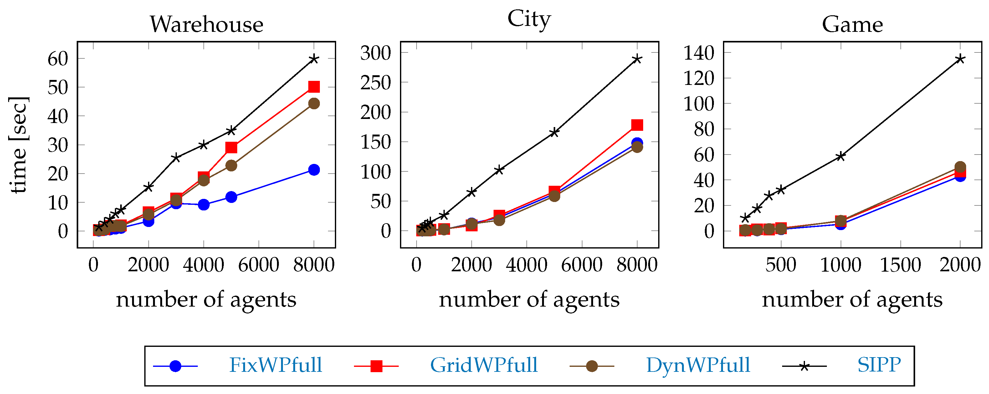
We denote the analysed hierarchical pathfinding methods FixWPfull, FixWPwin, DynWPfull, DynWPwin, GridWPfull, and GridWPwin. The first part of the notation indicates the hierarchical pathfinding method, the middle “WP” indicates “waypoint” pathfinding, and the ending indicates whether full or windowed pathfinding is used. The reference pathfinding method is the SIPP method. The best parameters of the waypoint proximity path planning method for the example scenarios of the competition in [5] were 24 for the maximum distance between waypoints, 8 for the proximity of the target waypoint path planning, and 12 for the closeness to the target waypoint when the agent aims towards the next waypoint. We use the same values in the tests.

There are several things that we want to test. We would like to test the solution quality of the hierarchical pathfinding methods in case of a single agent, the speed-up of hierarchical pathfinding in case of multiple agents, the robustness against emerging conflicts, and whether windowed or full pathfinding performs better in these aspects. We formulate hypotheses for these.

Hypothesis 1 (H1).

The length of the path with hierarchical pathfinding in a single agent scenario is maximum 1% more than the optimal solution.

The path smoothing of the original hierarchical pathfinder in [6] achieved 1% overhead, but in the LMAPF-T setting with reservations we use the waypoint proximity path planning method to smooth the path. We hope that the waypoint proximity path-planning method produces results similar to the path smoothing of the original hierarchical pathfinder.

The measurement to test this hypothesis is to count the number of steps needed to complete 1000 errands by a single agent in the example scenarios.

Hypothesis 2 (H2).

The one shot MAPF-T problem is computed faster with full path hierarchical pathfinding than with SIPP.

We expect that full path hierarchical pathfinding can find an initial solution of a MAPF-T problem faster than SIPP, and then the remaining time can be used for optimisation of the paths.

The measurement to test this hypothesis is the time needed to compute the first step of the example scenarios, and then we compare these values to the time of the SIPP computation.

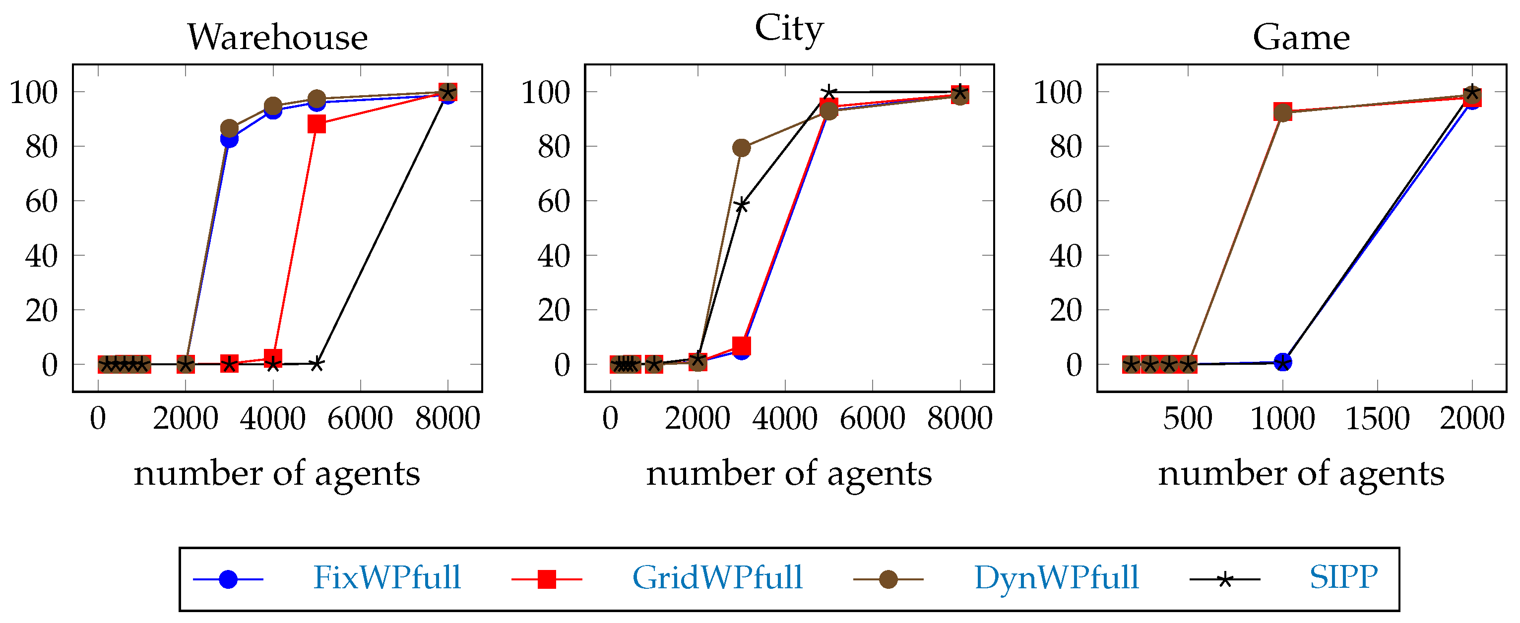
Hypothesis 3 (H3).

The LMAPF-T problem is computed faster with full path hierarchical pathfinding than with SIPP, but the gain quickly drops as the team size increases.

Although the MAPF-T hierarchical pathfinding is faster, we expect that the emerging conflicts to generate repeated path searches; therefore the average time of pathfinding quickly increases as the team size increases. We are not only interested in the average, but also in the timeouts to see if the slowdown is a general issue or if it is caused by only a few cases.

The measurements to test this hypothesis are the timeout percentage during the test execution, and the average pathfinding time during the test execution.

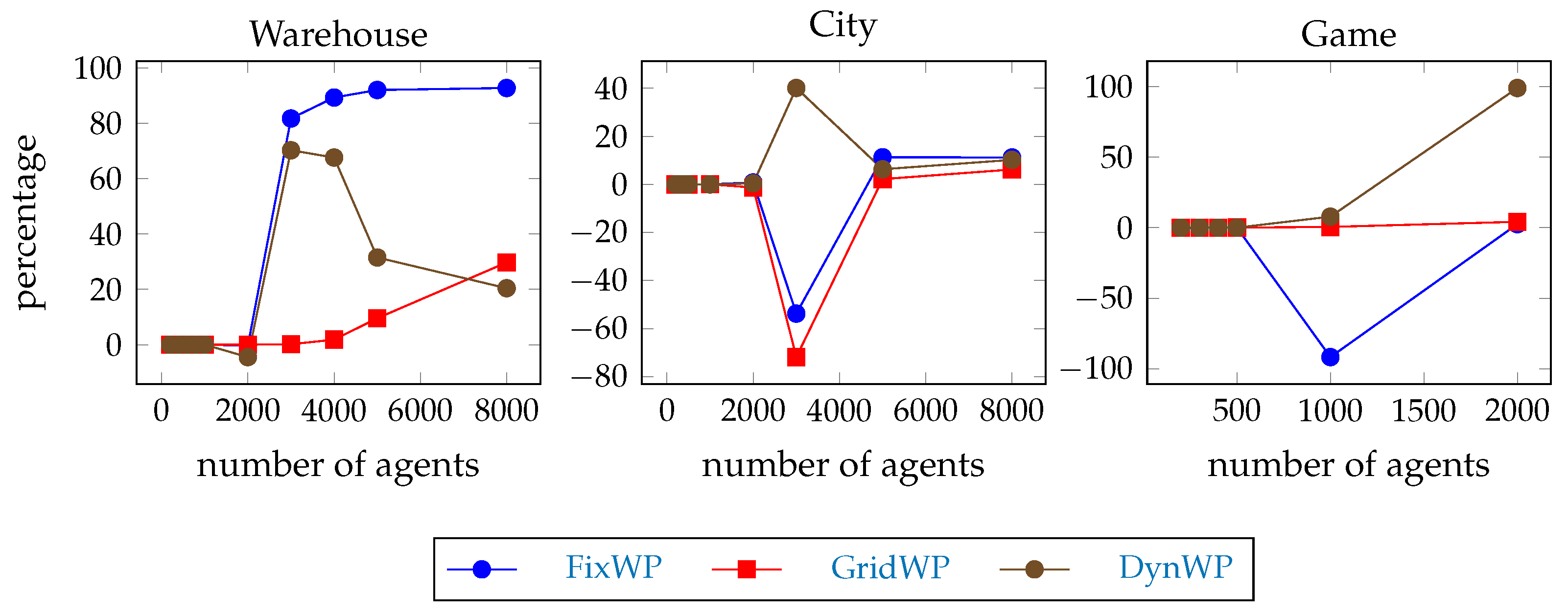
Hypothesis 4 (H4).

The throughput of the full path hierarchical pathfinding solution is worse than the throughput of the SIPP solution in general, but it is significant only if the agent team size is large.

We expect that the full path hierarchical pathfinding works faster, but the solution quality is not so good, and the robustness against emerging conflicts quickly drops if the team size increases; therefore the throughput is not better than the throughput of the SIPP solution.

The measurement to test this hypothesis is the number of errands completed per agent per 500 steps5 (i.e., 500 times the number of errands completed divided by the number of agents divided by the total number of steps in the experiment).

Hypothesis 5 (H5).

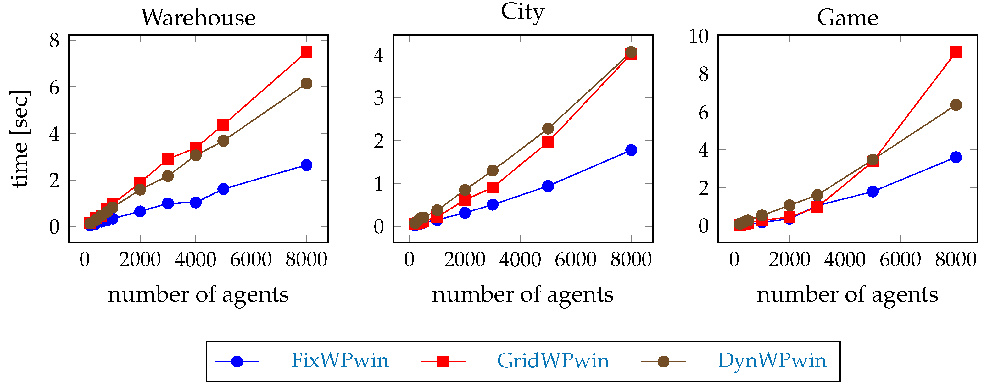
The LMAPF-T problem is computed faster with windowed hierarchical pathfinding than with full path hierarchical pathfinding.

We expect that the windowed hierarchical pathfinder is faster.

The measurements to test this hypothesis are the percentage of time steps with response time longer than 1 s during the test execution, and the average pathfinding time during the test execution compared to the full path hierarchical pathfinding results.

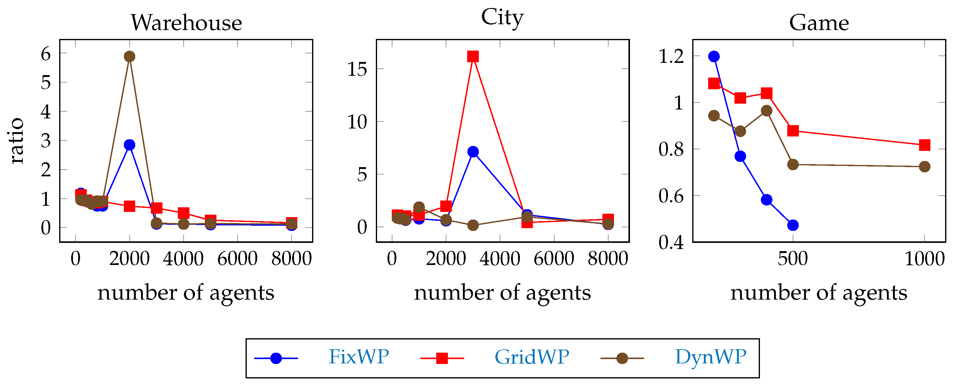
Hypothesis 6 (H6).

The throughput of the windowed hierarchical pathfinding solution is less than the throughput of the full path hierarchical pathfinder.

We expect that although the windowed hierarchical pathfinding works faster, but the solution quality is not so good, and the robustness against emerging conflicts is worse than in the case of full path hierarchical pathfinding; therefore the throughput is less than the throughput of the full path solution.

The measurement to test this hypothesis is the number of errands completed per agent per 500 steps as a ratio of the full path hierarchical pathfinding results.

5. Experimental Results

5.1. Single Agent Pathfinding

Hypothesis 1 (H1).

The length of the path with hierarchical pathfinding in a single agent scenario is maximum 1% more than the optimal solution.

The number of steps needed to complete 1000 errands by a single agent in the example scenarios are shown in

Table 1. Number of steps needed to complete 1000 errands with 1 agent.

Algorithm	City [Steps]	Game [Steps]	wh [Steps]
SIPP	197,167	439,684	241,968
FixWPfull	217,593	455,711	244,227
GridWPfull	217,593	455,711	244,227
DynWPfull	211,499	452,972	243,522

. The number of extra steps needed to complete 1000 errands by a single agent in the example scenarios compared to SIPP are shown in

Table 2. Number of extra steps needed to complete 1000 errands with 1 agent compared to SIPP.

Algorithm	City Extra [%]	Game Extra [%]	wh Extra [%]
FixWPfull	10.36%	3.65%	0.93%
GridWPfull	10.36%	3.65%	0.93%
DynWPfull	7.27%	3.02%	0.64%

. We can see that more than 7% extra steps are needed on the city map, and more than 3% extra steps are needed on the game map. The extra steps on the warehouse map are below 1%. Hypothesis H1 is refuted. In general, the path smoothing with waypoint proximity path planning, which is needed to handle the SIPP reservations, is not so efficient than the classic hierarchical path smoothing. The efficiency depends on the type of map. On the warehouse map the waypoint proximity path planning is efficient in this experiment.

5.2. Full Path Hierarchical Pathfinding

Hypothesis 2 (H2).

A one shot MAPF-T problem is computed faster with full path hierarchical pathfinding than with SIPP.

The time needed to compute the first step of the example scenarios is shown on Figure 6. The hierarchical pathfinders are faster than the SIPP. Hypothesis H2 is confirmed. The differences can be better seen in Figure 7 where the planning times are shown as the percentage of the SIPP planning time. The order depends on the type of map, but the GridWPfull pathfinder needs the most time among the hierarchical pathfinders, except on the game map.

Hypothesis 3 (H3).

The LMAPF-T problem is computed faster with full path hierarchical pathfinding than with SIPP, but the gain quickly drops as the team size increases.

The percentage of steps over the 1 s timeout during the test execution is shown on Figure 8. The timeouts clearly dominate at bigger team sizes. The limits are not so clear. On the warehouse map, the GridWPfull fails only at team size 5000, FixWPfull and DynWPfull already fail at team size 3000, the SIPP fails only above 5000. On the city map, GridWPfull and FixWPfull are more or less ok at team size 3000, but all of them fail at 5000. On the game map, FixWPfull and SIPP work at team size 1000, and all of them fail at team size 2000. Larger team sizes are not included because the execution time would have been too long due to our simple method of resolving emerging conflicts.

The average pathfinding time during the test execution with SIPP is shown in

Table 3. Average planning times during the test execution with SIPP.

(a) Warehouse
agents	avg time [s]
200	0.011998901
400	0.022552702
600	0.034176904
800	0.041371778
1000	0.050681986
2000	0.100927232
3000	0.151275545
4000	0.208499815
5000	0.285683670
8000	6.832577463
(b) City
agents	avg time [s]
200	0.045657797
300	0.067279897
400	0.088269814
500	0.105861575
1000	0.211923618
2000	0.396427745
3000	40.267597740
5000	40.134877420
(c) Game
agents	avg time [s]
200	0.039688620
300	0.060824621
400	0.084290686
500	0.100520674
1000	0.238721289
2000	66.859035690

. This is in line with the timeout results; so the increased average pathfinding time is a general issue. The average pathfinding time during the test execution with the full path hierarchical pathfinders is shown in Figure 9 as a percentage of the SIPP time. They produce useful speed-up only until team size 5000 on the city map, until team size 2000 on the warehouse map, and until team size 500 on the game map. This is also in line with the timeout results, so the increased average pathfinding time is a general issue. Hypothesis H3 is confirmed.

Hypothesis 4 (H4).

The throughput of the full-path hierarchical pathfinding solution is worse than that of the SIPP solution in general, but it is significant only if the agent team size is large.

The number of errands completed per agent per 500 steps is shown in Figure 10. SIPP has the highest throughput on all maps. On the warehouse map, the throughput of FixWPfull and DynWPfull drop at team size 2000, and GridWPfull drops at team size 5000. On the city map, all hierarchical pathfinders degrade above team size 3000. On the game map, GridWPfull and DynWPfull drop at team size 1000, and all of them drop above team size 1000. The performance drops at larger team sizes, so Hypothesis H4 is confirmed.

5.3. Windowed Hierarchical Pathfinding

Hypothesis 5 (H5).

The LMAPF-T problem is computed faster with windowed hierarchical pathfinding than with full path hierarchical pathfinding.

The timeout percentage of the windowed pathfinders during the test execution compared to the full path hierarchical pathfinding results are shown in Figure 11. Note that we call windowed pathfinders those that always plan only until the next waypoint, and the waypoint distances are at most 24 as described in Section 4. On the warehouse map, the full-path pathfinders produce more timeouts than the windowed pathfinders (with a small exception at team size 2000). On this map, the windowed versions of the FixWP and the DynWP methods are better than the GridWP method. On the city map, the windowed versions of the GridWP and FixWP methods are worse than the full-path versions at team size 3000, but otherwise the windowed versions are better. On the game map, the windowed version of the FixWP method is worse than the full-path version at team size 1000, but otherwise the windowed versions are better.

The time of the path planning in the first step of the example scenarios with windowed hierarchical pathfinding is shown in Figure 12. The values are obviously much smaller than with full-path pathfinding (see Figure 6) because the pathfinding is only until the first waypoint.

The average pathfinding time of the windowed hierarchical pathfinding during the test execution divided by the average pathfinding time of the full-path hierarchical pathfinding are shown in Figure 13. The results are not unanimous: although most of the cases the windowed hierarchical pathfinding methods work faster, but in many cases the full-path hierarchical pathfinders are better. Hypothesis H5 is refuted.

Hypothesis 6 (H6).

The throughput of the windowed hierarchical pathfinding solution is less than the throughput of the full-path hierarchical pathfinder.

The ratio of the number of errands completed per agent per 500 steps by the windowed hierarchical pathfinders divided by the number of errands completed per agent per 500 steps by the full-path hierarchical pathfinders is shown in Figure 14. The results are in line with this Hypothesis H6 in most of the cases, but there are a few exceptions on the game map at agent team size 1000, so Hypothesis H6 is refuted.

6. Evaluation

The experiments do not show an overall clear result. The results sometimes are specific to the given scenario. It is clear that one shot hierarchical pathfinding is faster than SIPP pathfinding, and the response time of the windowed hierarchical pathfinders is shorter than the response time of the full-path hierarchical pathfinders. However, on the longer run of the LMAPF-T problem, this faster response time often diminishes, probably because of the emerging conflicts of the LMAPF-T problem. In the experiments, the path planning time of the SIPP algorithm was the longest, then mainly the grid waypoint version was the second longest, and finally the fix and dynamic waypoint versions were the shortest. The throughput of the SIPP algorithm was the best, then the grid waypoint was mainly the second best, and the fix and dynamic waypoint versions were somewhat behind. Although the windowed hierarchical pathfinders have the best response time, their better throughput in connection with the SIPP algorithm cannot be confirmed.

7. Conclusions

One of the techniques to speed-up pathfinding on large maps is the hierarchical pathfinding. The hierarchical pathfinding algorithm is usually used to find the path for a single agent. A common technique in MAPF to use reservation tables to find conflict-free paths for multiple agents. It is called space–time search (CA*) or state–time search (SIPP). We have developed and formally presented three different techniques to use hierarchical pathfinding in connection with state–time search in LMAPF-T problems. We have evaluated these techniques using the example scenarios from the 2023 League of Robot Runners competition. According to the experiments, the hierarchical pathfinding techniques produce better response times in the beginning compared to the SIPP algorithm, but in the longer run they produce worse throughput. The windowed version of the hierarchical pathfinders produce the best response time, but this does not necessarily lead to better throughput.

In spite of these problems, the full-path hierarchical pathfinding methods can be used to produce an initial solution quickly, and then other techniques are needed to resolve the emerging conflicts and to optimise the conflict-free paths, like in large neighbour search.

The windowed hierarchical pathfinding methods can be used to improve the response time, but they may lose a bit on the throughput.