Remanufacturing Modes Selection in Competitive Closed-Loop Supply Chains

Abstract

In the context of green economy, Closed-Loop Supply Chain (CLSC) competition is intensifying. This study aims to help companies operating in green supply chains determine optimal remanufacturing strategies when competing with other firms. We examine the decision-making problem of CLSCs in competitive environments facing multiple remanufacturing mode options. The research constructs a Prisoner’s dilemma model for dual CLSCs, where each chain has three strategic choices: independent remanufacturing, outsourced remanufacturing, and authorized remanufacturing. Employing Stackelberg game models, Nash equilibrium analysis, and numerical simulations, this study explores how remanufactured product unit saving costs affect remanufacturing mode decisions concerning competitive intensity and discount policies. The study then draws the following conclusions: (1) CLSCs prefer outsourced and authorized remanufacturing in competitive scenarios; (2) Remanufactured product discounting significantly influences CLSC remanufacturing decisions; (3) Competitors typically adopt conservative strategies by aligning decisions with rivals. These results provide practical guidance for CLSCs selecting remanufacturing approaches when facing substitute competition, contributing to more sustainable and competitive supply chain operations.

1. Introduction

Competition for CLSCs is intensifying as global companies continue to focus on sustainability and environmental protection. Many companies are developing circular economy models that maximize the life of products through remanufacturing, as well as recycling and reusing materials at the end of their life cycle. Remanufacturing is an important means for the country to achieve the “carbon peak and carbon neutrality” goal and to promote the development of a green economy [1]. China first proposed the “Dual carbon” goal at the 75th session of the General Assembly of the United Nations. Considering the greenness and economy of remanufacturing, many enterprises and some Original Equipment Manufacturer (OEM) companies, such as Caterpillar, Xerox, EPSON, HP, IBM, and Michelin, have been actively involved in remanufacturing activities [2,3]. Remanufactured products not only extend the life cycle of products and reduce resource wastage, but also reduce production costs and environmental impacts. By reusing and reprocessing waste materials, remanufactured products provide an effective way for companies to achieve resource recycling, which helps to reduce carbon emissions and over-exploitation of natural resources. For instance, Nike has developed Nike Grind, a recycled material made from used sports shoes and production waste, which is used in the manufacture of new sports shoes and sports surfaces [4]. It has recycled 140 million pounds of waste materials since 1992. IKEA reduces resource consumption and environmental impact by recycling and reusing waste furniture materials to produce new furniture products [5].

Currently, remanufacturing models mainly include independent remanufacturing, outsourced remanufacturing and authorised remanufacturing. Independent remanufacturing refers to the production and sale of new and remanufactured products by OEM and Third-Party Remanufacturer (TPR) respectively, which are independent and compete with each other. Outsourced remanufacturing means that the OEM and the TPR are in a partnership, where the OEM outsources the remanufacturing activities to the TPR, thus focusing on the production of new products, but with pricing power for remanufactured products. For example, Land Rover outsources its remanufacturing activities to Caterpillar [6]. Authorized remanufacturing is another partnership model where the OEM authorises remanufacturing activities to TPR while the pricing of the remanufactured product is transferred to TPR. However, it is a major challenge for CLSCs to choose the optimal remanufacturing mode in the face of competition. Specifically, we address the following questions:

1. What is the optimal remanufacturing model decision for a CLSC in a competitive market?

2. Which factor, the intensity of market competition or the discount on remanufactured products, has a strong influence on the decision of a CLSC remanufacturing model?

3. When in a competitive market, should a CLSC choose a conservative strategy (aligned with the other party’s strategy) or a risky strategy (not aligned with the other party’s strategy)?

In competitive markets, the choice of remanufacturing model can have a significant impact on the profitability, market positioning, and sustainability of OEMs. The optimal decision depends on a number of key factors, such as unit savings from remanufacturing, competitive intensity, and discount of remanufactured products. In less competitive situations, OEMs may prefer an outsourced remanufacturing model to maximize control over pricing and quality. However, in highly competitive markets, authorized remanufacturing activities to TPRs tend to be more attractive because it allows OEMs to profit from licensing fees while avoiding a direct price war.

The intensity of market competition and the discount of remanufactured products both influence decision-making, but their relative importance varies. In markets with fierce competition, OEMs are more likely to adopt an authorized remanufacturing mode to stabilize prices and reduce rivalry. Conversely, when consumers highly value remanufactured products (i.e., the discount is small), OEMs may prioritize capturing the secondary market through outsourced remanufacturing. The balance between these factors determines whether an OEM should compete, cooperate, or abstain from remanufacturing altogether.

The choice between conservative and risky strategies depends on market stability and risk tolerance. A conservative approach—aligning with competitors’ strategies—reduces uncertainty and is preferable in volatile markets. However, if an OEM has a strong cost advantage or superior brand reputation, a risky strategy can lead to higher profits.

The rest of this paper is organized as follows: Section 2 reviews the relevant literatures. Section 3 introduces the notations and models used later on. Section 4 builds six Stackelberg models, respectively, and solves for the decision variables and the profit equilibrium solution for each subject. Section 5 introduces numerical experiments, which include the CLSC’s remanufacturing mode selection, impact of each parameter on decision-making, and profits of CLSCs. Section 6 includes some discussion and conclusions. The proofs of all corollaries are given in Appendix A.

2. Literature Review

Our research is mainly related to these two streams of literature: (1) remanufacturing model; (2) CLSC competition. Table 1 provides a summary of the pertinent literature, emphasizing key research gaps that our paper seeks to address.

2.1. Remanufacturing Model

At present, scholars have carried out a series of studies on remanufacturing model research and achieved certain results. This paper reviewed relevant research on remanufacturing models from three perspectives. The first is outsourced remanufacturing: Fang et al. [7] described the definition of outsourced remanufacturing, which is a commonly adopted business practice in which OEMs outsource remanufacturing to Third-Party Remanufacturers (TPRs) and focus on new products. Yan et al. [8] concluded that outsourcing is more beneficial to manufacturers by comparing and analyzing the economic, social, and environmental status quo under the two modes of OEMs and TPRs, but failed to gain the support of manufacturers. Zhao et al. [9] on the basis of information asymmetry of enterprises, using evolutionary game theory, studied the recovery strategy of outsourcing of remanufacturing enterprises, which provides reference for enterprises’ long-term outsourced remanufacturing decision.

The second is authorized remanufacturing: The subject of authorizing fee decision-making is not necessarily the OEM, Zhou et al. [10] studied three bargaining scenarios for authorizing decision-making: fee setting by the OEM, fee setting by the contract manufacturer, and fee setting by mutual negotiation, and concluded that neither exogenous nor endogenous wholesale prices could lead to authorizing cooperation. Liu et al. [11] argued that the quality of small remanufactured products relying on in-house research and development is often lower than that of established OEMs, and that authorizing of patents by OEMs is expected to improve the quality of remanufactured products. Huang et al. [12] modeled the impact of competition between new products and authorized and unauthorized remanufactured products on OEMs’ marketing and channel strategies.

The third is remanufacturing model selection: In the early CLSC, manufacturing companies mainly recovered used products for product remanufacturing through direct recycling, retailer recycling and third-party recycling [13]. Zou et al. [14] focused on comparing the two modes of authorized remanufacturing and outsourced remanufacturing. Huang et al. [15] classified the remanufacturing model into supplier-remanufacturing and manufacturer-remanufacturing and developed a Stackelberg model to analyze the supply chain member profit relationships. Feng et al. [16] constructed two remanufacturing models dominated by OEM and independent remanufacturer (IR) and further explored the impact of government subsidies on both models. Zhou et al. [17] proposed the self-remanufacturing model, in which the OEM performs its own remanufacturing activities. Li et al. [18] further examined the impact of tax and duty regulations on an OEM’s decision whether to engage in remanufacturing or outsource to a TPR. Ma et al. [19] explored the issue of financing strategies for OEMs to choose between outsourced remanufacturing model or authorized remanufacturing model.

In contrast to the above literatures, we considered three modes of decision making: independent remanufacturing, authorised remanufacturing, and outsourced remanufacturing under competitive conditions. We also considered the impact of multiple factors on the decision-making model of remanufacturing, including the intensity of competition in the market, the discount of remanufactured products, and the remanufactured product unit saving costs.

2.2. CLSC Competition

In this paper, we reviewed related studies on competition in CLSCs from two perspectives. The first is the pricing [20,21,22], coordination [23,24] and network equilibrium decision-making literature [25,26,27,28] on CLSCs. For example, Gu et al. [29] discovered that government subsidies significantly enhance the sustainable development of CLSCs across economic, environmental and social dimensions. Through Stackelberg game analysis of manufacturer-retailer-collector systems, they found subsidies consistently improve total chain profits, environmental benefits and social welfare, with more pronounced effects under unequal bargaining power structures. Wang et al. [30] investigated government intervention mechanisms in CLSC coordination, comparing reward-penalty and subsidy mechanisms. Their analysis of centralized versus decentralized models revealed that both can enhance collection rates and partner profits while reducing new product prices when environmental benefits are moderate. Cheng et al. [31] revealed that cap-sharing schemes outperform cap-and-trade in balancing profitability and emission reduction in multi-tiered CLSCs. Their variational inequality model showed scientifically allocated emission caps with green technology incentives optimize network performance, especially for large enterprises. Taleizadeh et al. [32] discovered that channel power structures significantly influence optimal pricing, quality, and return policies in three-level CLSCs.

The second one is the study of market structure and firm competition in CLSCs, which examines the competitive strategies of firms in CLSCs under different market structures. Pal et al. [33] explored the competition between two different qualitative substitutes in a CLSC. Wang et al. [34] developed a game model to explore the effect of incentives and penalties on the competition of substitutes and concluded that the recovery rate is positively related to the coefficient of substitution. Doustmohammadi and Babazadeh [35] examined the competition of CLSC substitutes in the WPC industry. Zhang et al. [36] explored price competition for patented substitutes in a CLSC. Wei et al. [37] explored the optimal collection strategy for a CLSC consisting of a manufacturer, a retailer and two collectors, where the two collectors are in competition. It is concluded that when competition is intense, it is more beneficial for the retailer to merge with the collectors. Liu et al. [22] explored a CLSC consisting of a competing manufacturer and a single retailer, which found that the greater the competition, the greater the CLSC profits.

Most of the above literatures consider competition in a single CLSC. The studies that consider dual CLSCs do not incorporate the Nash equilibrium analysis to dynamically analyze the equilibrium solution, despite using the Stackelberg model. Our main contributions are listed below (Table 1): First, combining these two streams of literature, we considered the choice of remanufacturing model in two CLSCs under a competitive market. And we analyzed the dynamics of the model equilibrium solution using the delineation method. Second, we explored the effects of market competition intensity, remanufacturing discounts, and unit savings on decision-making in remanufacturing models.

Table 1. Comparison of our work with related literature.

Papers	Model Formulation		Decision Variables		Strategy
	RM	CC	PQ	PP	SM
Yan et al. [8]	✓	×	✓	✓	×
Zhao et al. [9]	✓	×	✓	×	✓
Mutha et al. [13]	×	×	✓	✓	×
Huang et al. [15]	✓	×	×	✓	✓
Li et al. [18]	✓	×	✓	✓	✓
Xu et al. [22]	×	✓	✓	✓	×
Pal et al. [32]	×	✓	×	✓	✓
Doustmohammadi and Babazadeh [34]	×	✓	×	×	×
Zhang et al. [35]	✓	✓	×	✓	✓
Liu et al. [37]	×	✓	×	✓	×
Our research	✓	✓	✓	✓	✓

Note: RM = remanufacturing mode; CC = CLSC competition; PQ = Product quantity; PP = Product price; SM = Stackelberg Model.

Table 1. Comparison of our work with related literature.

Papers	Model Formulation		Decision Variables		Strategy
	RM	CC	PQ	PP	SM
Yan et al. [8]	✓	×	✓	✓	×
Zhao et al. [9]	✓	×	✓	×	✓
Mutha et al. [13]	×	×	✓	✓	×
Huang et al. [15]	✓	×	×	✓	✓
Li et al. [18]	✓	×	✓	✓	✓
Xu et al. [22]	×	✓	✓	✓	×
Pal et al. [32]	×	✓	×	✓	✓
Doustmohammadi and Babazadeh [34]	×	✓	×	×	×
Zhang et al. [35]	✓	✓	×	✓	✓
Liu et al. [37]	×	✓	×	✓	×
Our research	✓	✓	✓	✓	✓

Note: RM = remanufacturing mode; CC = CLSC competition; PQ = Product quantity; PP = Product price; SM = Stackelberg Model.

3. Model

To examine competitive decision-making in CLSCs, we developed a Prisoner’s dilemma framework involving two parallel CLSCs, each consisting of an OEM and a Third-Party Remanufacturer (TPR) producing substitute products. The model distinctly segregates production responsibilities: OEMs exclusively manufacture new products while TPRs specialize in remanufactured products, with both distributing directly to consumers. This segregation ensures clarity and efficiency in the production processes within each CLSC. Each CLSC offers three distinct remanufacturing models: independent remanufacturing, outsourced remanufacturing, and authorised remanufacturing, so there are nine strategies in total. Because the two CLSC costs are homogeneous, the profit matrix is symmetric along the diagonal, and this paper unfolds the six strategies: Model II, Model IO, Model IA, Model OO, Model OA and Model AA, which are structured as shown below Figure 1. Our study specifically explored how remanufactured product unit saving costs affect remanufacturing model decisions across varying levels of market competition intensity and remanufactured product discounts, providing comprehensive insights into competitive CLSC dynamics.

The main assumptions about costs, product life, consumers, authorised remanufacturing mode and outsourced remanufacturing mode in this paper are as follows.

Table 2. Notations.

Notations	Definitions
Indices
i	Index of the Model: $i\in \{II,IO,IA,OO,OA,AA\}$
j	Index of the products: $j=n$ (new products); $j=r$ (remanufactured products)
k	Index of the CLSC: $k\in \{1,2\}$
Symbols
s	Unit saving costs of new and remanufactured products
c	Unit production costs of new products
$\delta$	Discount on remanufactured products
$\beta$	Intensity of competition
Decision variables
$p_{jk}^i$	Indicates the retail price per unit of j in CLSC k under Model i
$q_{jk}^i$	Indicates the market demand of j in CLSC k under Model i
$z_k$	Unit license fee under CLSC k
$w_k$	Unit outsourcing fee under CLSC k

shows the notations used in this paper.

Let s and c denote the unit saving costs of new and remanufactured products and unit production costs of the new products, respectively. According to the related literature [38], the cost of manufacturing remanufactured products is lower than the cost of manufacturing new products, that is, s exists and satisfies: $0<s<c$. The inequality ensures the economic viability of remanufacturing, while it reflects the fundamental cost advantage that makes remanufacturing an attractive alternative to conventional production.

All events take place within a single period. We presume the product was already present in the market. The quantity of remanufactured products should not exceed that of used products that can be gathered from consumers within a single period [39]. Therefore, the new and remanufactured product quantities satisfy: $q_{nk}^i⩾q_{rk}^i$.

Consumers’ willingness to pay v for new products is assumed to obey a uniform distribution on $[0,1]$. Specifically, the net utility gained by consumers from purchasing the new product is $U_{nk}=v-p_{nk}$. Consistent with the related literatures [40,41], consumers generally have a lower willingness-to-pay for remanufactured products. The consumer’s valuation discount on remanufactured products is denoted by $\delta (0<\delta <1)$. The consumer’s net utility from purchasing remanufactured products is $U_{rk}=\delta v-p_{rk}$. Furthermore, $\beta (0<\beta <1)$ indicates the intensity of competition in the market, and as the value increases, the competition becomes more intense [42]. A consumer possesses a maximum of one item, either new or remanufactured, with the market size standardized to 1. Therefore, the inverse demand function of the new and remanufactured products of two products can be formulated as follows:

$$p_{n1}^i=1-(q_{n1}^i+\delta q_{r1}^i)-\beta (q_{n2}^i+\delta q_{r2}^i)$$

(1)

$$p_{r1}^i=\delta (1-(q_{n1}^i+q_{r1}^i)-\beta (q_{n2}^i+q_{r2}^i))$$

(2)

$$p_{n2}^i=1-(q_{n2}^i+\delta q_{r2}^i)-\beta (q_{n1}^i+\delta q_{r1}^i)$$

(3)

$$p_{r2}^i=\delta (1-(q_{n2}^i+q_{r2}^i)-\beta (q_{n1}^i+q_{r1}^i))$$

(4)

In order to acquire authorization for selling remanufactured products, the TPR must pay the unit authorizing fee $z_1$ or $z_2$ ($z_1>0,z_2>0$) to the OEM [43]. This fee is an exogenous variable set by the OEM and remains unaffected by the demand for remanufactured products; OEM outsourcing the production of remanufactured products to TPR is required to pay the unit outsourcing fee $w_1$ or $w_2$ ($w_1>0,w_2>0$) to TPR [19]. This fee is an exogenous variable set by the TPR and remains unaffected by the demand for remanufactured products.

4. Model Formulation

There are nine strategies in total, but due to homogeneity, the strategy matrix is symmetrically distributed along the diagonal, so the model only shows six strategies. In this paper, we developed a two-stage decision model to analyze the strategic interaction between OEMs and Third-Party Remanufacturers (TPRs). At the same time, the reverse induction approach is used to solve this continuous game: the remaining equilibrium solutions are obtained first by computing the second-stage equilibrium solutions and then substituting these equilibrium solutions into the first-stage model.

4.1. Model II: Both Independent Remanufacturing Mode

In this scenario, both OEMs take independent remanufacturing model, with the OEMs profiting from the sale of new products and the TPRs profiting from the sale of remanufactured products. The two OEMs and TPRs profit equations are shown below:

$${\pi }_{n1}^{II}=(p_{n1}^{II}-c)q_{n1}^{II}$$

(5)

$${\pi }_{r1}^{II}=(p_{r1}^{II}-c+s)q_{r1}^{II}$$

(6)

$${\pi }_{n2}^{II}=(p_{n2}^{II}-c)q_{n2}^{II}$$

(7)

$${\pi }_{r2}^{II}=(p_{r2}^{II}-c+s)q_{r2}^{II}$$

(8)

The two OEMs first make simultaneous decisions on the demand for new product 1 and 2, followed by the two TPRs making simultaneous decisions on the demand for remanufactured products 1 and 2. Applying reverse induction, the optimal solutions for Model II are as follows:

Lemma 1.

In the Model II, the equilibrium market demand for new product 1, 2, remanufactured product 1, 2 and the profits of OEMs, TPRs are given as follows:

$$q_{n1}^{I{I}^{*}}=q_{n2}^{I{I}^{*}}={\displaystyle \frac{(\beta -2)\left(\right(s+\delta -1)\beta +s+\delta +c-2)}{(\delta -1){\beta }^3-2{\beta }^2+(4-3\delta )\beta -4\delta +8}}$$

(9)

$$\begin{array}{cc}\hfill q_{r1}^{I{I}^{*}}=q_{r2}^{I{I}^{*}}=& {\displaystyle \frac{(c-s-c\delta ){\beta }^3+((-c-1)\delta +2c-2s){\beta }^2}{(\beta +2)\delta \left((\delta -1){\beta }^3-2{\beta }^2+(4-3\delta )\beta -4\delta +8\right)}}\hfill \\ \hfill & +{\displaystyle \frac{+(4c\delta -4c+4s)\beta -2{\delta }^2+(6c-2s+4)\delta -8c+8s}{(\beta +2)\delta \left((\delta -1){\beta }^3-2{\beta }^2+(4-3\delta )\beta -4\delta +8\right)}}\hfill \end{array}$$

(10)

$${\pi }_{n1}^{I{I}^{*}}={\pi }_{n2}^{I{I}^{*}}={\displaystyle \frac{(\beta -2){((s+\delta -1)\beta +s+\delta +c-2)}^2\left({\beta }^2+2\delta -4\right)}{{\left((\delta -1){\beta }^3-2{\beta }^2+(4-3\delta )\beta -4\delta +8\right)}^2(\beta +2)}}$$

(11)

$${\pi }_{r1}^{I{I}^{*}}=\left(\delta \left(1-\left(q_{n1}^{I{I}^{*}}+\delta q_{r1}^{I{I}^{*}}\right)-\beta \left(q_{n2}^{I{I}^{*}}+\delta q_{r2}^{I{I}^{*}}\right)\right)-c+s\right)q_{r1}^{I{I}^{*}}$$

(12)

$${\pi }_{r2}^{I{I}^{*}}=\left(\delta \left(1-\left(q_{n2}^{I{I}^{*}}+\delta q_{r2}^{I{I}^{*}}\right)-\beta \left(q_{n1}^{I{I}^{*}}+\delta q_{r1}^{I{I}^{*}}\right)\right)-c+s\right)q_{r2}^{I{I}^{*}}$$

(13)

4.2. Model IO: One Is Independent Remanufacturing Mode, the Other Is Outsourced Remanufacturing Mode

In this scenario, OEM1 chooses the independent remanufacturing model and OEM2 chooses the outsourced remanufacturing model. The profits of each of the two OEMs and TPRs are shown below:

$${\pi }_{n1}^{IO}=(p_{n1}^{IO}-c)q_{n1}^{IO}$$

(14)

$${\pi }_{r1}^{IO}=(p_{r1}^{IO}-c+s)q_{r1}^{IO}$$

(15)

$${\pi }_{n2}^{IO}=(p_{n2}^{IO}-c)q_{n2}^{IO}+(p_{r2}^{IO}-w_2)q_{r2}^{IO}$$

(16)

$${\pi }_{r2}^{IO}=(w_2-c+s)q_{r2}^{IO}$$

(17)

When OEM1 decides on the demand for new product 1, TPR2 decides on the unit outsourcing fee for remanufactured product 2. Next, when TPR1 decides on the demand for remanufactured product 1, OEM2 decides on the demand for both new product 2 and remanufactured product 2.

Lemma 2.

In the Model IO, the equilibrium market demand for new product 1, 2, remanufactured product 1, 2, and unit remanufacturing outsourcing cost need to satisfy the following equations, and the profits of OEMs and TPRs are given as follows:

$$-\delta q_{r1}^{I{O}^{*}}+\delta \left(1-q_{n1}^{I{O}^{*}}-q_{r1}^{I{O}^{*}}-\beta \left(q_{n2}^{I{O}^{*}}+q_{r2}^{I{O}^{*}}\right)\right)-c+s=0$$

(18)

$$-2q_{n2}^{I{O}^{*}}+1-2\delta q_{r2}^{I{O}^{*}}-\beta \left(\delta q_{r1}^{I{O}^{*}}+q_{n1}^{I{O}^{*}}\right)-c=0$$

(19)

$$-\delta q_{n2}^{I{O}^{*}}-\delta q_{r2}^{I{O}^{*}}+\delta \left(1-q_{n2}^{I{O}^{*}}-q_{r2}^{I{O}^{*}}-\beta \left(q_{r1}^{I{O}^{*}}+q_{n1}^{I{O}^{*}}\right)\right)-w_2^{*}=0$$

(20)

$$\begin{array}{cc}\hfill & {\displaystyle \frac{-2q_{n1}^{I{O}^{*}}(\delta -1){\beta }^4+\left(c-w_2+\delta -1\right){\beta }^3+\beta \left(-4c+2w_2-2\delta +4\right)-8}{2{\beta }^2-8}}\hfill \\ \hfill & +{\displaystyle \frac{\left(\left(8q_{n1}^{I{O}^{*}}-2\right)\delta -2s-12q_{n1}^{I{O}^{*}}+2\right){\beta }^2+\left(8q_{n1}^{I{O}^{*}}+4\right)\delta +4c+4s+16q_{n1}^{I{O}^{*}}}{2{\beta }^2-8}}=0\hfill \end{array}$$

(21)

$$\begin{array}{cc}\hfill & {\displaystyle \frac{\left({\beta }^3{\delta }^2{q}_{n1}^{I{O}^{*}}-{\beta }^3\delta q_{n1}^{I{O}^{*}}-{\beta }^2\delta c-{\beta }^2{\delta }^2+{\beta }^2\delta w_2^{*}-2\beta {\delta }^2{q}_{n1}^{I{O}^{*}}+{\beta }^2\delta -2\beta \delta c+2\beta c+2\beta \delta s+\right.}{2\delta \left({\beta }^2-4\right)(\delta -1)}}\hfill \\ \hfill & +{\displaystyle \frac{\left.2\beta \delta q_{n1}^{I{O}^{*}}-2\beta \delta -2\beta s+4c\delta -4w_2^{*}\right)+\left(w_2^{*}-c+s\right)\left({\beta }^2\delta -4\right)}{2\delta \left({\beta }^2-4\right)(\delta -1)}}=0\hfill \end{array}$$

(22)

$${\pi }_{n1}^{I{O}^{*}}=\left(\left(1-\left(q_{n1}^{I{0}^{*}}+\delta q_{r1}^{I{O}^{*}}\right)-\beta \left(q_{n2}^{I{O}^{*}}+\delta q_{r2}^{I{O}^{*}}\right)\right)-c\right)q_{n1}^{I{O}^{*}}$$

(23)

$${\pi }_{r1}^{I{O}^{*}}=\left(\delta \left(1-\left(q_{n1}^{{I_{*}}^{*}}+\delta q_{r1}^{I{O}^{*}}\right)-\beta \left(q_{n2}^{I{O}^{*}}+\delta q_{r2}^{I{O}^{*}}\right)\right)-c+s\right)q_{r1}^{I{O}^{*}}$$

(24)

$${\pi }_{n2}^{I{O}^{*}}=(p_{n2}^{I{O}^{*}}-c)q_{n2}^{I{O}^{*}}+(p_{r2}^{I{O}^{*}}-w_2^{*})q_{r2}^{I{O}^{*}}$$

(25)

$${\pi }_{r2}^{I{O}^{*}}=(w_2^{*}-c+s)q_{r2}^{I{O}^{*}}$$

(26)

4.3. Model IA: One Is Independent Remanufacturing Mode, the Other Is Authorised Remanufacturing Mode

In this scenario, OEM1 selects the independent remanufacturing model and OEM2 selects the authorised remanufacturing model. The two OEMs and TPRs profit formulas are as follows:

$${\pi }_{n1}^{IA}=(p_{n1}^{IA}-c)q_{n1}^{IA}$$

(27)

$${\pi }_{r1}^{IA}=(p_{r1}^{IA}-c+s)q_{r1}^{IA}$$

(28)

$${\pi }_{n2}^{IA}=(p_{n2}^{IA}-c)q_{n2}^{IA}+z_2{q}_{r2}^{IA}$$

(29)

$${\pi }_{r2}^{IA}=(p_{r2}^{IA}-c+s-z_2)q_{r2}^{IA}$$

(30)

Firstly, when OEM1 decides on the new product 1 demand, OEM2 decides on the unit licencing fee of remanufactured product 2; secondly, when TPR1 decides on the remanufactured product 1 demand, OEM2 decides on the new product 2 demand and finally TPR2 decides on the remanufactured product 2 demand.

Lemma 3.

In the Model IA, the equilibrium market demand for new product 1, 2, remanufactured product 1, 2, unit licence cost need to satisfy the following equations and the profits of OEMs, TPRs are given as follows:

$$\begin{array}{c}\hfill {\displaystyle \frac{\left(-s-2q_{n1}^{I{A}^{*}}-\delta +1\right){\beta }^2+\left(2-4q_{n1}^{I{A}^{*}}\right)\delta +2c+2s+8q_{n1}^{I{A}^{*}}}{{\beta }^2-4}}\\ \hfill +{\displaystyle \frac{\left(\left(-3q_{n2}^{I{A}^{*}}+1\right)\delta -c+s-z_2^{*}+4q_{n2}^{I{A}^{*}}\right)\beta -4+q_{n2}^{I{A}^{*}}(\delta -1){\beta }^3}{{\beta }^2-4}}=0\end{array}$$

(31)

$$\begin{array}{cc}\hfill & {\displaystyle \frac{\left(-s-2q_{n2}^{I{A}^{*}}-\delta +1\right){\beta }^2+\left(2-4q_{n2}^{I{A}^{*}}\right)\delta +2c+2s+8q_{n2}^{I{A}^{*}}}{{\beta }^2-4}}\hfill \\ \hfill & +{\displaystyle \frac{\left(\left(-3q_{n1}^{I{A}^{*}}+1\right)\delta -c+s+4q_{n1}^{I{A}^{*}}\right)\beta -4+q_{n1}^{I{A}^{*}}(\delta -1){\beta }^3}{{\beta }^2-4}}=0\hfill \end{array}$$

(32)

$$-\delta q_{r1}^{I{A}^{*}}+\delta \left(1-q_{n1}^{I{A}^{*}}-q_{r1}^{I{A}^{*}}-\beta \left(q_{n2}^{I{A}^{*}}+q_{r2}^{I{A}^{*}}\right)\right)-c+s=0$$

(33)

$$-\delta q_{r2}^{I{A}^{*}}+\delta \left(1-q_{n2}^{I{A}^{*}}-\delta q_{r2}^{I{A}^{*}}-\beta \left(q_{n1}^{I{A}^{*}}+q_{r1}^{I{A}^{*}}\right)\right)-c+s-z_2^{*}=0$$

(34)

$${\displaystyle \frac{\left(\left(q_{n1}^{I{A}^{*}}+1\right)\delta -c+s\right)\beta +2c-2s+4z_2^{*}-2\delta }{\delta \left({\beta }^2-4\right)}}=0$$

(35)

$${\pi }_{n1}^{I{A}^{*}}=(p_{n1}^{I{A}^{*}}-c)q_{n1}^{I{A}^{*}}$$

(36)

$${\pi }_{r1}^{I{A}^{*}}=(p_{r1}^{I{A}^{*}}-c+s)q_{r1}^{I{A}^{*}}$$

(37)

$${\pi }_{n2}^{I{A}^{*}}=(p_{n2}^{I{A}^{*}}-c)q_{n2}^{I{A}^{*}}+z_2^{*}{q}_{r2}^{IA}$$

(38)

$${\pi }_{r2}^{I{A}^{*}}=(p_{r2}^{I{A}^{*}}-c+s-z_2^{*})q_{r2}^{I{A}^{*}}$$

(39)

4.4. Model OO: Both Outsourced Remanufacturing Mode

In this scenario, both OEMs take outsourced remanufacturing model, with the OEMs profiting from sales of new and remanufactured products. TPRs profits from the outsourcing fee. The profit equations for both OEMs and TPRs are shown below:

$${\pi }_{n1}^{OO}=(p_{n1}^{OO}-c)q_{n1}^{OO}+(p_{r1}^{OO}-w_1)q_{r1}^{OO}$$

(40)

$${\pi }_{r1}^{OO}=(w_1-c+s)q_{r1}^{OO}$$

(41)

$${\pi }_{n2}^{OO}=(p_{n2}^{OO}-c)q_{n2}^{OO}+(p_{r2}^{OO}-w_2)q_{r2}^{OO}$$

(42)

$${\pi }_{r2}^{OO}=(w_2-c+s)q_{r2}^{OO}$$

(43)

The two TPRs first decide on the unit outsourcing fee, followed by the two OEMs deciding on the demand for new and remanufactured products.

Lemma 4.

In the Model OO, the equilibrium market demand for new product 1, 2, remanufactured product 1, 2, unit remanufacturing outsourcing cost need to satisfy the following equations and the profits of OEMs, TPRs are given as follows:

$$-2q_{n1}^{O{O}^{*}}+1-2\delta q_{r1}^{O{O}^{*}}-\beta \left(q_{n2}^{O{O}^{*}}+\delta q_{r2}^{O{O}^{*}}\right)-c=0$$

(44)

$$-2q_{n2}^{O{O}^{*}}+1-2\delta q_{r2}^{O{O}^{*}}-\beta \left(q_{n1}^{O{O}^{*}}+\delta q_{r1}^{O{O}^{*}}\right)-c=0$$

(45)

$$-\delta q_{n1}^{O{O}^{*}}-\delta q_{r1}^{O{O}^{*}}+\delta \left(1-q_{n1}^{O{O}^{*}}-q_{r1}^{O{O}^{*}}-\beta \left(q_{n2}^{O{O}^{*}}+q_{r2}^{O{O}^{*}}\right)\right)-w_1^{*}=0$$

(46)

$$-\delta q_{n2}^{O{O}^{*}}-\delta q_{r2}^{O{O}^{*}}+\delta \left(1-q_{n2}^{O{O}^{*}}-q_{r2}^{O{O}^{*}}-\beta \left(q_{n1}^{O{O}^{*}}+q_{r1}^{O{O}^{*}}\right)\right)-w_1^{*}=0$$

(47)

$${\displaystyle \frac{-c(\beta -2)\delta +\beta w_2^{*}+2c-2s-4w_1^{*}}{\delta \left({\beta }^2-4\right)(\delta -1)}}=0$$

(48)

$${\displaystyle \frac{-c(\beta -2)\delta +\beta w_1^{*}+2c-2s-4w_2^{*}}{\delta \left({\beta }^2-4\right)(\delta -1)}}=0$$

(49)

$${\pi }_{n1}^{O{O}^{*}}=(p_{n1}^{O{O}^{*}}-c)q_{n1}^{O{O}^{*}}+(p_{r1}^{O{O}^{*}}-w_1^{*})q_{r1}^{O{O}^{*}}$$

(50)

$${\pi }_{r1}^{O{O}^{*}}=(w_1^{*}-c+s)q_{r1}^{O{O}^{*}}$$

(51)

$${\pi }_{n2}^{O{O}^{*}}=(p_{n2}^{O{O}^{*}}-c)q_{n2}^{O{O}^{*}}+(p_{r2}^{O{O}^{*}}-w_2^{*})q_{r2}^{O{O}^{*}}$$

(52)

$${\pi }_{r2}^{O{O}^{*}}=(w_2^{*}-c+s)q_{r2}^{O{O}^{*}}$$

(53)

4.5. Model OA: One Is Outsourced Remanufacturing Mode, the Other Is Authorised Remanufacturing Mode

In this scenario, when OEM1 selects the outsourced remanufacturing model, OEM2 selects the authorised remanufacturing model. The two OEMs and TPRs profit equations are shown below:

$${\pi }_{n1}^{OA}=(p_{n1}^{OA}-c)q_{n1}^{OA}+(p_{r1}^{OA}-w_1)q_{r1}^{OA}$$

(54)

$${\pi }_{r1}^{OA}=(w_1-c+s)q_{r1}^{OA}$$

(55)

$${\pi }_{n2}^{OA}=(p_{n2}^{OA}-c)q_{n2}^{OA}+z_2{q}_{r2}^{OA}$$

(56)

$${\pi }_{r2}^{OA}=(p_{r2}^{OA}-c+s-z_2)q_{r2}^{OA}$$

(57)

First, when TPR1 decides on the outsourcing cost per unit of remanufactured product 1, OEM2 decides on the licensing cost per unit of remanufactured product 2; second, when OEM1 decides on the demand for new product 1 and remanufactured product 1, OEM2 decides on the demand for new product 2; and finally, TPR2 decides on the demand for remanufactured product 2.

Lemma 5.

In the Model OA, the equilibrium market demand for new product 1, 2, remanufactured product 1, 2, unit remanufacturing outsourcing cost, unit licence cost need to satisfy the following equations and the profits of OEMs, TPRs are given as follows:

$$-2q_{n1}^{O{A}^{*}}+1-2\delta q_{r1}^{O{A}^{*}}-\beta \left(q_{n2}^{O{A}^{*}}+\delta q_{r2}^{O{A}^{*}}\right)-c=0$$

(58)

$$\begin{array}{c}\hfill {\displaystyle \frac{4c+4s+16q_{n2}^{O{A}^{*}}-8+\left(c-w_1+\delta -1\right){\beta }^3+{\beta }^2\left(\left(8q_{n2}^{O{A}^{*}}-2\right)\delta -2s-12q_{n2}^{O{A}^{*}}+2\right)}{2{\beta }^2-8}}\\ \hfill +{\displaystyle \frac{\left(4c+2w_1^{*}-2\delta +4\right)\beta +\left(-8q_{n2}^{O{A}^{*}}+4\right)\delta +-2q_{n2}^{O{A}^{*}}(\delta -1){\beta }^4}{2{\beta }^2-8}}=0\end{array}$$

(59)

$$-\delta q_{n1}^{O{A}^{*}}-\delta q_{r1}^{O{A}^{*}}+\delta \left(1-q_{n1}^{O{A}^{*}}-q_{r1}^{O{A}^{*}}-\beta \left(q_{n2}^{O{A}^{*}}+q_{r2}^{O{A}^{*}}\right)\right)-w_1^{*}=0$$

(60)

$$-\delta q_{r2}^{O{A}^{*}}+\delta \left(1-q_{n2}^{O{A}^{*}}-\delta q_{r2}^{O{A}^{*}}-\beta \left(q_{n1}^{O{A}^{*}}+q_{r1}^{O{A}^{*}}\right)\right)-c+s-z_2^{*}=0$$

(61)

$$\begin{array}{cc}\hfill & {\displaystyle \frac{\left({\beta }^3{\delta }^2{q}_{n1}^{O{A}^{*}}-{\beta }^3\delta q_{n1}^{O{A}^{*}}-{\beta }^2\delta c-{\beta }^2{\delta }^2+{\beta }^2\delta w_1^{*}-2\beta {\delta }^2{q}_{n1}^{O{A}^{*}}+{\beta }^2\delta -2\beta \delta c+2\beta c\right.}{2\delta \left({\beta }^2-4\right)(\delta -1)}}\hfill \\ \hfill & +{\displaystyle \frac{\left.2\beta \delta s+2\beta {\delta }^2+2\beta \delta q_{n1}^{O{A}^{*}}-2\beta \delta -2\beta s+4c\delta -4w_1^{*}\right)+\left(w_1^{*}-c+s\right)\left({\beta }^2\delta -4\right)}{2\delta \left({\beta }^2-4\right)(\delta -1)}}=0\hfill \end{array}$$

(62)

$${\pi }_{n1}^{O{A}^{*}}=(p_{n1}^{O{A}^{*}}-c)q_{n1}^{O{A}^{*}}+(p_{r1}^{O{A}^{*}}-w_1^{*})q_{r1}^{O{A}^{*}}$$

(63)

$${\pi }_{r1}^{O{A}^{*}}=(w_1^{*}-c+s)q_{r1}^{O{A}^{*}}$$

(64)

$${\pi }_{n2}^{O{A}^{*}}=(p_{n2}^{O{A}^{*}}-c)q_{n2}^{O{A}^{*}}+z_2^{*}{q}_{r2}^{O{A}^{*}}$$

(65)

$${\pi }_{r2}^{O{A}^{*}}=(p_{r2}^{O{A}^{*}}-c+s-z_2^{*})q_{r2}^{O{A}^{*}}$$

(66)

4.6. Model AA: Both Authorised Remanufacturing Mode

In this scenario, both OEMs take the authorised remanufacturing model, where the OEMs profit from new product sales and licensing fee. TPRs profit from remanufactured product sales. The profit equations for the OEMs and TPRs are shown below:

$${\pi }_{n1}^{AA}=(p_{n1}^{AA}-c)q_{n1}^{AA}+z_1{q}_{r1}^{AA}$$

(67)

$${\pi }_{r1}^{AA}=(p_{r1}^{AA}-c+s-z_1)q_{r1}^{AA}$$

(68)

$${\pi }_{n2}^{AA}=(p_{n2}^{AA}-c)q_{n2}^{AA}+z_2{q}_{r2}^{AA}$$

(69)

$${\pi }_{r2}^{AA}=(p_{r2}^{AA}-c+s-z_2)q_{r2}^{AA}$$

(70)

The two OEMs decide on the unit licence fee and then on the demand for new products 1 and 2, while at the same time the two TPRs decide on the demand for remanufactured products 1 and 2.

Lemma 6.

In the Model AA, the equilibrium market demand for new product 1, 2, remanufactured product 1, 2, unit licence cost need to satisfy the following equations and the profits of OEMs, TPRs are given as follows:

$$\begin{array}{cc}\hfill & {\displaystyle \frac{\left(-s-2q_{n1}^{A{A}^{*}}-\delta +1\right){\beta }^2+\left(2-4q_{n1}^{A{A}^{*}}\right)\delta +2c+2s+8q_{n1}^{A{A}^{*}}}{{\beta }^2-4}}\hfill \\ \hfill & +{\displaystyle \frac{\left(\left(-3q_{n2}^{A{A}^{*}}+1\right)\delta -c+s-z_2^{*}+4q_{n2}^{A{A}^{*}}\right)\beta -4+q_{n2}^{A{A}^{*}}(\delta -1){\beta }^3}{{\beta }^2-4}}=0\hfill \end{array}$$

(71)

$$\begin{array}{cc}\hfill & {\displaystyle \frac{\left(-s-2q_{n2}^{A{A}^{*}}-\delta +1\right){\beta }^2+\left(2-4q_{n2}^{A{A}^{*}}\right)\delta +2c+2s+8q_{n2}^{A{A}^{*}}}{{\beta }^2-4}}\hfill \\ \hfill & +{\displaystyle \frac{\left(\left(-3q_{n1}^{A{A}^{*}}+1\right)\delta -c+s-z_1^{*}+4q_{n1}^{A{A}^{*}}\right)\beta -4+q_{n1}^{A{A}^{*}}(\delta -1){\beta }^3}{{\beta }^2-4}}=0\hfill \end{array}$$

(72)

$$-\delta q_{r1}^{A{A}^{*}}+\delta \left(1-q_{n1}^{A{A}^{*}}-\delta q_{r1}^{A{A}^{*}}-\beta \left(q_{n2}^{A{A}^{*}}+q_{r2}^{A{A}^{*}}\right)\right)-c+s-z_1^{*}=0$$

(73)

$$-\delta q_{r2}^{A{A}^{*}}+\delta \left(1-q_{n2}^{A{A}^{*}}-\delta q_{r2}^{A{A}^{*}}-\beta \left(q_{n1}^{A{A}^{*}}+q_{r1}^{A{A}^{*}}\right)\right)-c+s-z_2^{*}=0$$

(74)

$${\displaystyle \frac{\left(\left(q_{n2}^{A{A}^{*}}+1\right)\delta -c+s-z_2^{*}\right)\beta +2c-2s+4z_1^{*}-2\delta }{\delta \left({\beta }^2-4\right)}}=0$$

(75)

$${\displaystyle \frac{\left(\left(q_{n1}^{A{A}^{*}}+1\right)\delta -c+s-z_1^{*}\right)\beta +2c-2s+4z_2^{*}-2\delta }{\delta \left({\beta }^2-4\right)}}=0$$

(76)

$${\pi }_{n1}^{A{A}^{*}}=(p_{n1}^{A{A}^{*}}-c)q_{n1}^{A{A}^{*}}+z_1^{*}{q}_{r1}^{A{A}^{*}}$$

(77)

$${\pi }_{r1}^{A{A}^{*}}=(p_{r1}^{A{A}^{*}}-c+s-z_1^{*})q_{r1}^{A{A}^{*}}$$

(78)

$${\pi }_{n2}^{A{A}^{*}}=(p_{n2}^{A{A}^{*}}-c)q_{n2}^{A{A}^{*}}+z_2^{*}{q}_{r2}^{A{A}^{*}}$$

(79)

$${\pi }_{r2}^{A{A}^{*}}=(p_{r2}^{A{A}^{*}}-c+s-z_2^{*})q_{r2}^{A{A}^{*}}$$

(80)

5. Numerical Analysis

In this Section we used numerical experiments to analyze the equilibrium solutions from Section 4. The intensity of market competition $\beta$ takes values between (0, 1). When $\beta$ is close to 0, there is almost no substitutability of products. Taking $\beta =0.8$ allows for the most intensely competitive markets; taking $\beta =0.5$ reflects a partially homogeneous market, which is consistent with the classical duopoly model of competition, such as the automobile industry (e.g., Toyota vs. Honda) [44]; and the interval of 0.3 clearly distinguishes the degree of competition, so we take $\beta =0.2$ [45,46,47]. When $\beta =0.2$, products are highly differentiated and competition is weak—e.g., Rolex vs. Patek Philippe—with brand reputation and unique features limiting direct price competition [48]. The discounts of remanufactured products $\delta \in (0<\delta <1)$ reflect consumers’ willingness to pay for a remanufactured product relative to a new product. The higher $\delta$ indicates a lower level of discounting. When $\delta =0.2$, remanufactured products face steep discounts. For instance, recycled automotive components like alternators that cost even more to recycle than new products [49]. At $\delta =0.5$, we observed moderate discounts common for certified refurbished consumer electronics such as smartphones or laptops, where professional refurbishment and limited warranties help maintain about half the value of new devices [50]. The highest $\delta$ value (0.8) applies to premium remanufactured goods that retain most of their functionality and brand value, exemplified by networking equipment like Cisco routers [51]. These differential discount rates are well-documented in the literature [40,41], our choice of $\delta \in \left\{0.2,0.5,0.8\right\}$ can cover most market situations. In order to satisfy the two conditions that both decision variables are greater than 0 and the number of new products is greater than the number of remanufactured products, s needs to be satisfied: $s\in [\underline{s},\overline{s}]$, fixing $c=0.8$ [14,41].

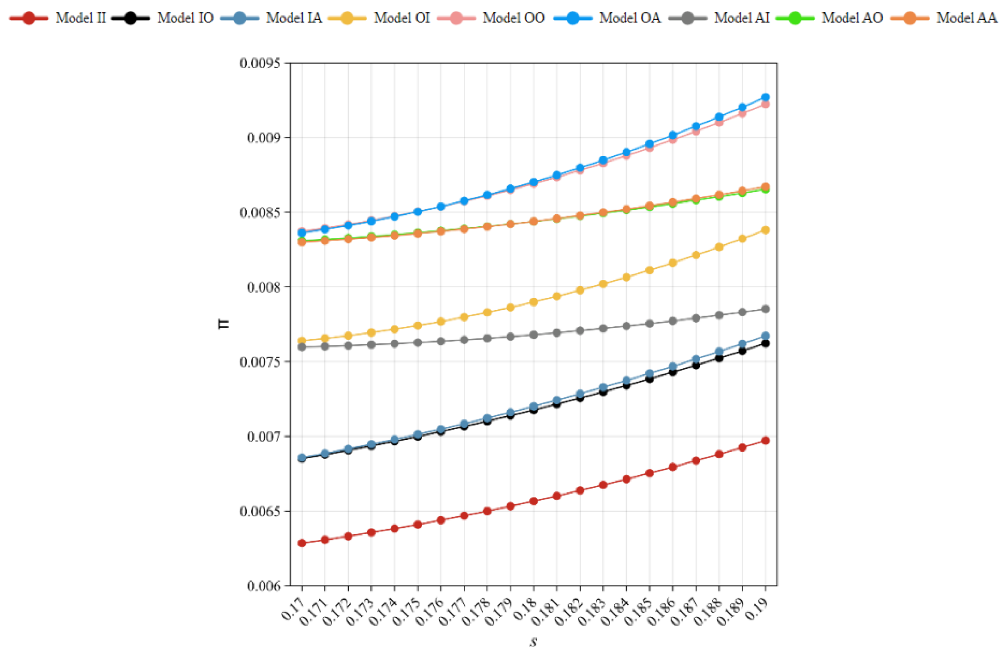
We first explore the low-competition and high-discount scenario, where the competition intensity is low $(\beta =0.2)$ and the discount factor is high $(\delta =0.2)$. This situation represents an industry environment with limited competitive pressure but substantial production cost savings in remanufacturing, which may reduce manufacturers’ incentives for proactive remanufacturing investments. In this setting, s takes the range $\left[0.645,0.655\right]$ (See Appendix A for details), testing how unit savings affect behavior.

Corollary 1.

In a low-competition, high-discount market environment, CLSC can maximize own profits by choosing outsourced remanufacturing mode.

(1) $s\in [0.645,0.654)$, take $s=0.649$, the profits of the CLSC remanufacturing model are as follows

Table 3. When $s=0.649$, remanufacturing modes profit.

CLSC1	CLSC2
	I Model	O Model	A Model
I model	(0.007771, 0.007771)	(0.007992, 0.0081)	(0.007998, 0.00811)
O model	(0.0081, 0.007992)	(0.008351, 0.008351)	(0.008335, 0.008345)
A model	(0.00811, 0.007998)	(0.008345, 0.008335)	(0.008343, 0.008343)

:

(2) Take $s=0.654$, the profits of the CLSC remanufacturing model are as follows

Table 4. When $s=0.654$, remanufacturing modes profit.

CLSC1	CLSC2
	I Model	O Model	A Model
I model	(0.00789, 0.00789)	(0.008158, 0.008177)	(0.008167, 0.008181)
O model	(0.008177, 0.008158)	(0.008473, 0.008473)	(0.008459, 0.008458)
A model	(0.008181, 0.008167)	(0.008458, 0.008459)	(0.008458, 0.008458)

:

(3) $s\in (0.654,0.655]$, take $s=0.655$, the profits of the CLSC remanufacturing model are as follows

Table 5. When $s=0.655$, remanufacturing modes profit.

CLSC1	CLSC2
	I Model	O Model	A Model
I model	(0.007921, 0.007921)	(0.008199, 0.008198)	(0.008209, 0.008201)
O model	(0.008198, 0.008199)	(0.008504, 0.008504)	(0.00849, 0.008486)
A model	(0.008201, 0.008209)	(0.008486, 0.00849)	(0.008487, 0.008487)

:

Combined with the analysis of the Nash equilibrium scribing method in Figure 2, it can be concluded that the optimal strategy is the outsourcing remanufacturing mode under the condition of low competition and high discount. This is because in the case of high discounts, the profit obtained by remanufacturing is very small, and there is no need to invest too much effort in the remanufacturing market. By outsourcing remanufacturing activities, OEMs can not only seize the remanufactured market, but also concentrate on producing new products, thereby gaining a greater advantage in a low-competition market.

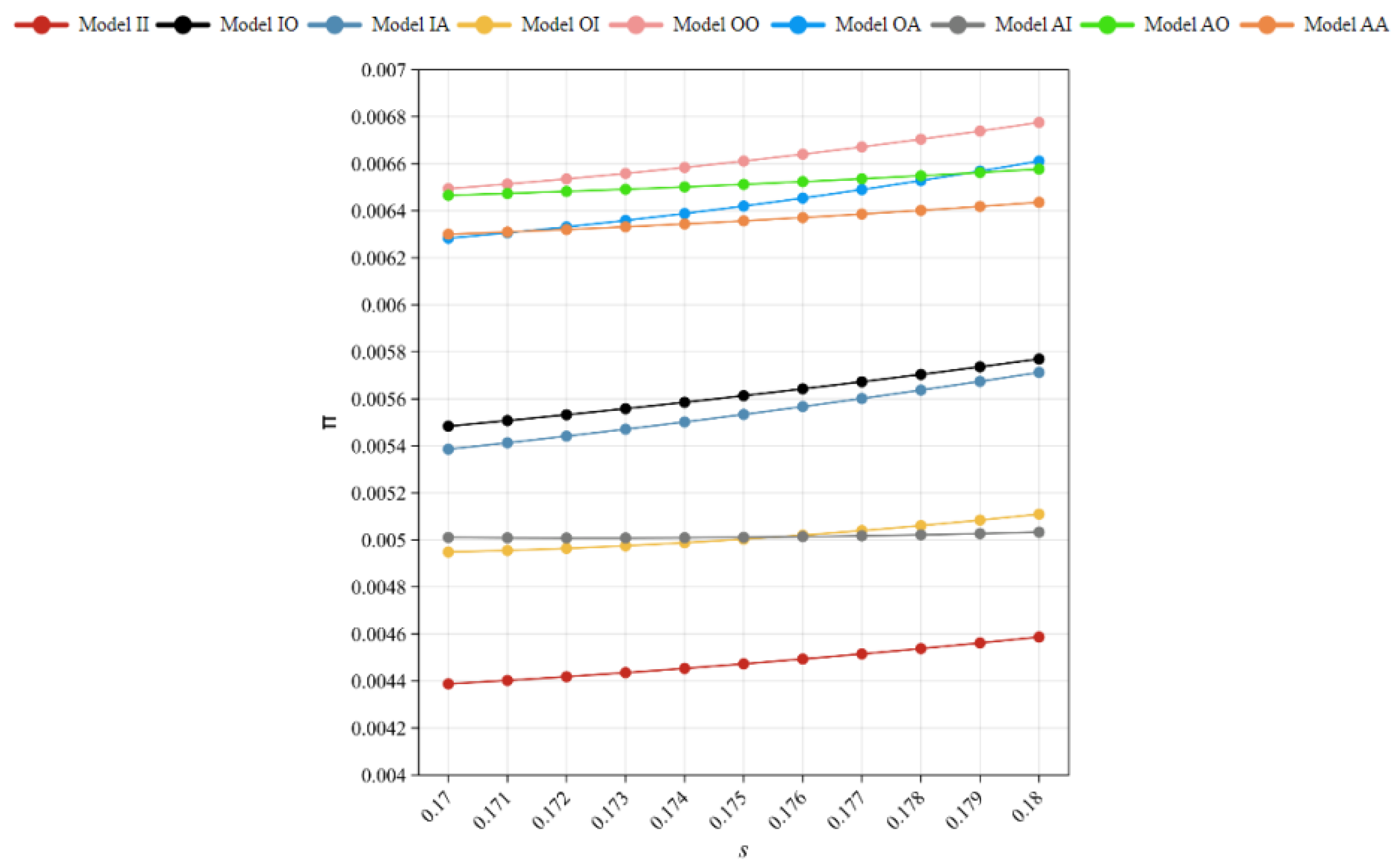
We next examine the low-competition and mid-discount scenario, where competition intensity remains low $(\beta =0.2)$ while the remanufacturing discount factor is moderate $(\delta =0.5)$. This reflects a market with limited rivalry but a balanced cost advantage for remanufactured products, resulting in intermediate incentives for strategic investments in remanufacturing. In this situation, $s\in [0.41,0.43]$. The following corollary can be made:

Corollary 2.

The optimal strategy for CLSC in a low-competition, mid-discount market is outsourced remanufacturing mode.

(1) $s\in [0.41,0.425)$, take $s=0.417$, the profits of the CLSC remanufacturing model are as follows

Table 6. When $s=0.417$, remanufacturing modes profit.

CLSC1	CLSC2
	I Model	O Model	A Model
I model	(0.007112, 0.007112)	(0.007579, 0.007911)	(0.007595, 0.007886)
O model	(0.007911, 0.007579)	(0.008462, 0.008462)	(0.008451, 0.008411)
A model	(0.007886, 0.007595)	(0.008411, 0.008451)	(0.00841, 0.00841)

:

(2) Take $s=0.425$, the profits of the CLSC remanufacturing model are as follows

Table 7. When $s=0.425$, remanufacturing modes profit.

CLSC1	CLSC2
	I Model	O Model	A Model
I model	(0.007346, 0.007346)	(0.007872, 0.008077)	(0.007897, 0.008002)
O model	(0.008077, 0.007872)	(0.008691, 0.008691)	(0.008688, 0.00858)
A model	(0.008002, 0.007897)	(0.00858, 0.008688)	(0.008586, 0.008586)

:

(3) $s\in (0.425,0.429)$, take $s=0.427$, the profits of the CLSC remanufacturing model are as follows

Table 8. When $s=0.427$, remanufacturing modes profit.

CLSC1	CLSC2
	I Model	O Model	A Model
I model	(0.007921, 0.007921)	(0.008199, 0.008198)	(0.008209, 0.008201)
O model	(0.008198, 0.008199)	(0.008504, 0.008504)	(0.00849, 0.008486)
A model	(0.008201, 0.008209)	(0.008486, 0.00849)	(0.008487, 0.008487)

:

(4) Take $s=0.429$, the profits of the CLSC remanufacturing model are as follows

Table 9. When $s=0.429$, remanufacturing modes profit.

CLSC1	CLSC2
	I Model	O Model	A Model
I model	(0.007496, 0.007496)	(0.008052, 0.008192)	(0.008083, 0.008083)
O model	(0.008192, 0.008052)	(0.008838, 0.008838)	(0.00884, 0.008689)
A model	(0.008083, 0.008083)	(0.008689, 0.00884)	(0.008699, 0.008699)

:

(5) $s\in (0.429,0.43]$, take $s=0.43$, the profits of the CLSC remanufacturing model are as follows

Table 10. When $s=0.43$, remanufacturing modes profit.

CLSC1	CLSC2
	I Model	O Model	A Model
I model	(0.007537, 0.007537)	(0.0081, 0.008224)	(0.008133, 0.008106)
O model	(0.008224, 0.0081)	(0.008878, 0.008878)	(0.008882, 0.008719)
A model	(0.008106, 0.008133)	(0.008719, 0.008882)	(0.00873, 0.00873)

:

As Figure 3, OEMs are still willing to focus on new products to improve market competitiveness when there is low-competition and mid-discount. Due to higher consumer preference for remanufactured products, OEMs prefer to retain pricing power over remanufactured products when handing over remanufacturing activities to Third-Party Remanufacturers (TPRs), i.e., they prefer the outsourced remanufacturing model.

We then investigate the low-competition and low-discount scenario, featuring weak market competition $(\beta =0.2)$ and a modest cost differential between new and remanufactured products $(\delta =0.8)$. This configuration reflects a market with limited competitive pressure where remanufacturing offers relatively small unit cost savings $(s\in [0.17,0.19\left]\right)$. Our study focuses on how these specific cost savings affect the CLSCs’ overall profitability.

Corollary 3.

The optimal strategy for the CLSC in the low-competition, low-discount scenario is still outsourced remanufacturing mode.

(1) $s\in [0.17,0.178)$, take $s=0.174$, the profits of the CLSC remanufacturing model are as follows

Table 11. When $s=0.174$, remanufacturing modes profit.

CLSC1	CLSC2
	I Model	O Model	A Model
I model	(0.006382, 0.006382)	(0.006966, 0.007717)	(0.006979, 0.00762)
O model	(0.007717, 0.006966)	(0.008473, 0.008473)	(0.00847, 0.00835)
A model	(0.00762, 0.006979)	(0.00835, 0.00847)	(0.008344, 0.008344)

:

(2) Take $s=0.178$, the profits of the CLSC remanufacturing model are as follows

Table 12. When $s=0.178$, remanufacturing modes profit.

CLSC1	CLSC2
	I Model	O Model	A Model
I model	(0.0065, 0.0065)	(0.007102, 0.007829)	(0.007122, 0.007656)
O model	(0.007829, 0.007102)	(0.00861, 0.00861)	(0.008616, 0.008405)
A model	(0.007656, 0.007829)	(0.008405, 0.008616)	(0.008403, 0.008403)

:

(3) $s\in (0.178,0.19]$, take $s=0.184$, the profits of the CLSC remanufacturing model are as follows

Table 13. When $s=0.184$, remanufacturing modes profit.

CLSC1	CLSC2
	I Model	O Model	A Model
I model	(0.006713, 0.006713)	(0.00734, 0.008065)	(0.007374, 0.007738)
O model	(0.008065, 0.00734)	(0.008878, 0.008878)	(0.008902, 0.008514)
A model	(0.007738, 0.007374)	(0.008514, 0.008902)	(0.00852, 0.00852)

:

When competition is low, OEMs prefer third-party remanufacturing (as Figure 4). Mid-discount and low-discount have little effect on the OEM’s remanufacturing model decision, and the OEM still prefers the outsourced remanufacturing model.

We next analyze the mid-competition and high-discount scenario, characterized by moderate market competition $(\beta =0.5)$ coupled with significant cost advantages for remanufactured products $(\delta =0.2)$. This parameter configuration depicts an industry environment with balanced competitive pressure where remanufacturing offers substantial unit cost savings. In this scenario, $s\in [0.645,0.655]$.

Corollary 4.

The optimal strategy for CLSC when in a mid-competition, high-discount market is authorised remanufacturing mode.

(1) $s\in [0.645,0.646)$, take $s=0.645$, the profits of the CLSC remanufacturing model are as follows

Table 14. When $s=0.645$, remanufacturing modes profit.

CLSC1	CLSC2
	I Model	O Model	A Model
I model	(0.005829, 0.005829)	(0.006192, 0.005825)	(0.006162, 0.006015)
O model	(0.005825, 0.006192)	(0.006423, 0.006423)	(0.006198, 0.00645)
A model	(0.006015, 0.006162)	(0.00645, 0.006198)	(0.00639, 0.00639)

:

(2) Take $s=0.646$, the profits of the CLSC remanufacturing model are as follows

Table 15. When $s=0.646$, remanufacturing modes profit.

CLSC1	CLSC2
	I Model	O Model	A Model
I model	(0.00583, 0.00583)	(0.006208, 0.005819)	(0.00618, 0.00601)
O model	(0.005819, 0.006208)	(0.006434, 0.006434)	(0.006209, 0.006459)
A model	(0.00601, 0.00618)	(0.006459, 0.00601)	(0.0064, 0.0064)

:

(3) $s\in (0.646,0.655]$, take $s=0.65$, the profits of the CLSC remanufacturing model are as follows in

Table 16. When $s=0.65$, remanufacturing modes profit.

CLSC1	CLSC2
	I Model	O Model	A Model
I model	(0.005851, 0.005851)	(0.006296, 0.00581)	(0.006273, 0.006002)
O model	(0.00581, 0.006296)	(0.006494, 0.006494)	(0.006271, 0.006514)
A model	(0.006002, 0.006273)	(0.006514, 0.006271)	(0.006458, 0.006458)

:

As shown in the above Figure 5, when in the mid-competition, OEMs will focus more on new product manufacturing to improve competitiveness. Due to the high discount of remanufactured products, OEMs do not tend to take the pricing power of remanufactured products into their own hands, and prefer to authorize thethe remanufacturing model at this time.

We then examine the mid-competition and mid-discount scenario, characterized by balanced market competition $(\beta =0.5)$ and intermediate cost advantages for remanufactured products $(\delta =0.5)$. This situation represents an industry environment with moderate competitive pressure where remanufacturing provides measurable but not substantial unit cost savings $(s\in [0.41,0.42\left]\right)$. We can draw the following Corollary:

Corollary 5.

In a market with mid-competition and mid-discount, the optimal strategy authorizedzed remanufacturing mode when the unit savings are small; when the savings are large, the optimal strategy is outsourced remanufacturing mode.

(1) $s\in [0.41,0.413)$, take $s=0.412$, the profits of the CLSC remanufacturing model are as follows

Table 17. When $s=0.412$, remanufacturing modes profit.

CLSC1	CLSC2
	I Model	O Model	A Model
I model	(0.005075, 0.005075)	(0.005896, 0.005341)	(0.005853, 0.005477)
O model	(0.005341, 0.005896)	(0.006487, 0.006487)	(0.006268, 0.006492)
A model	(0.005477, 0.005853)	(0.006492, 0.006268)	(0.006386, 0.006386)

:

(2) Take $s=0.413$, the profits of the CLSC remanufacturing model are as follows

Table 18. When $s=0.413$, remanufacturing modes profit.

CLSC1	CLSC2
	I Model	O Model	A Model
I model	(0.005084, 0.005084)	(0.005918, 0.005341)	(0.005877, 0.005475)
O model	(0.005341, 0.005918)	(0.0065015, 0.0065015)	(0.006284, 0.0065024)
A model	(0.005475, 0.005877)	(0.0065024, 0.006284)	(0.006398, 0.006398)

:

(3) $s\in (0.413,0.42]$, take $s=0.417$, the profits of the CLSC remanufacturing model are as follows

Table 19. When $s=0.417$, remanufacturing modes profit.

CLSC1	CLSC2
	I Model	O Model	A Model
I model	(0.005131, 0.005131)	(0.006019, 0.00535)	(0.005988, 0.005476)
O model	(0.00535, 0.006019)	(0.006574, 0.006574)	(0.006363, 0.006555)
A model	(0.005476, 0.005988)	(0.006555, 0.006363)	(0.006457, 0.006457)

:

According to the Figure 6, when the cost savings are small, the profit margins on remanufactured products are small and OEMs do not tend to retain pricing rights on remanufactured products, thus choosing the authorised remanufacturing model, however, when the cost savings are high, the increase in profit margins makes the OEMs more willing to retain pricing rights, and at this point, they prefer to choose outsourced remanufacturing model.

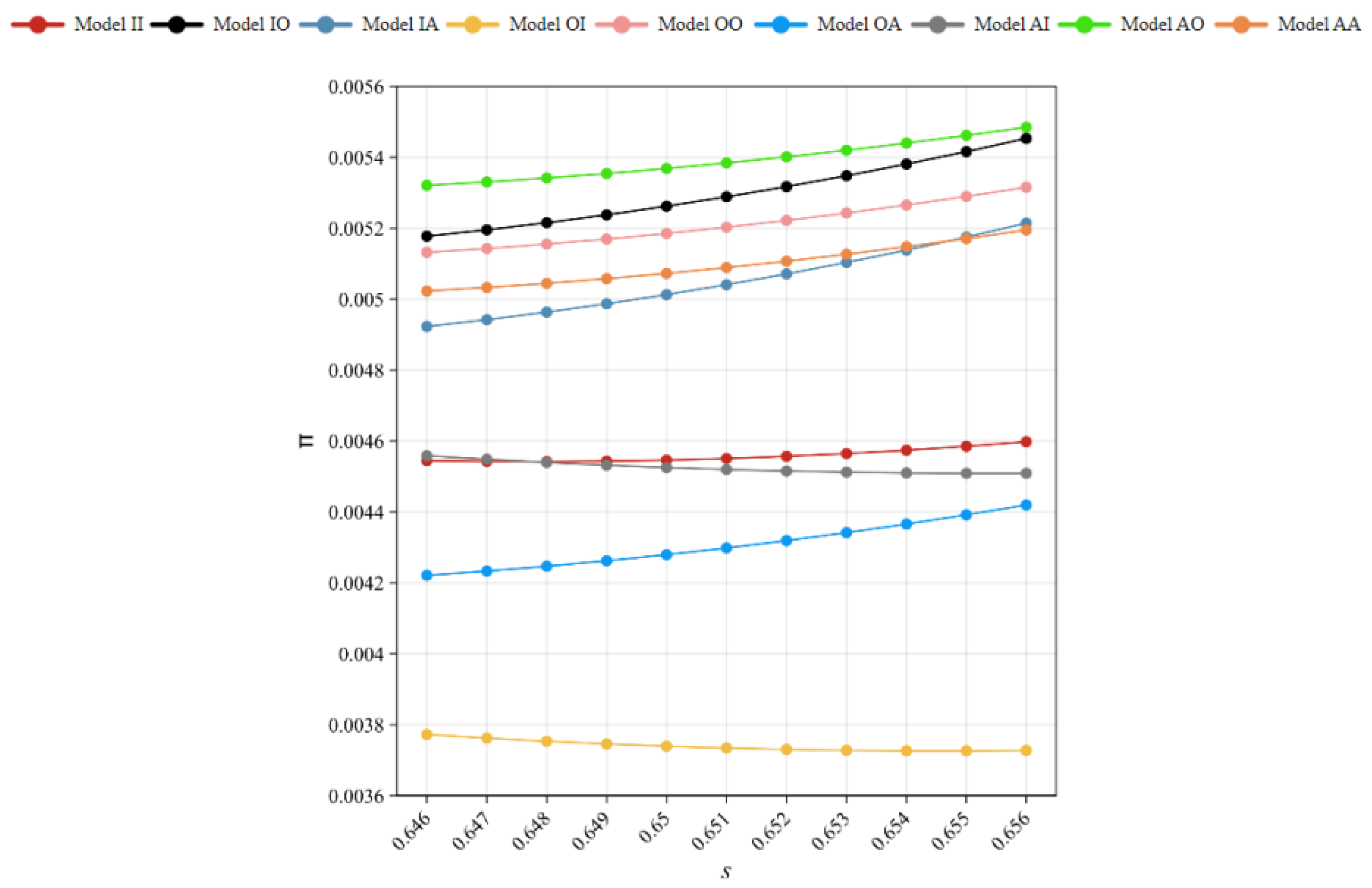
Our analysis now turns to the mid-competition, low-discount scenario, where market competition maintains a medium intensity level $(\beta =0.5)$ while the cost benefits derived from remanufacturing remain comparatively modest $(\delta =0.8)$. This particular configuration models an industrial setting that strikes a balance between competitive forces and production economics—sufficient competition exists to influence market dynamics, yet the economic incentives for remanufacturing are constrained by the relatively narrow cost differential between new and remanufactured products, creating distinct operational challenges for CLSC management. In this situation, $s\in [0.17,0.18]$. The corollary is as follows:

Corollary 6.

When the CLSC is in a mid-competition, low-discount market, the optimal strategy is outsourced remanufacturing mode.

(1) $s\in [0.17,0.171)$, take $s=0.17$, the profits of the CLSC remanufacturing model are as follows

Table 20. When $s=0.17$, remanufacturing modes profit.

CLSC1	CLSC2
	I Model	O Model	A Model
I model	(0.004388, 0.004388)	(0.005484, 0.004948)	(0.005386, 0.005011)
O model	(0.004948, 0.005484)	(0.006494, 0.006494)	(0.006283, 0.006466)
A model	(0.005011, 0.005386)	(0.006466, 0.006283)	(0.0063, 0.0063)

:

(2) Take $s=0.171$, the profits of the CLSC remanufacturing model are as follows

Table 21. When $s=0.171$, remanufacturing modes profit.

CLSC1	CLSC2
	I Model	O Model	A Model
I model	(0.004402 0.004402)	(0.005507, 0.004955)	(0.005413, 0.005009)
O model	(0.004955, 0.005507)	(0.006514, 0.006514)	(0.006306, 0.006473)
A model	(0.005009, 0.005413)	(0.006473, 0.006306)	(0.00631, 0.00631)

:

(3) $s\in (0.171,0.175)$, take $s=0.173$, the profits of the CLSC remanufacturing model are as follows

Table 22. When $s=0.173$, remanufacturing modes profit.

CLSC1	CLSC2
	I Model	O Model	A Model
I model	(0.004435, 0.004435)	(0.005558, 0.004975)	(0.005471, 0.005008)
O model	(0.004975, 0.005558)	(0.006559, 0.006559))	(0.006359, 0.006491)
A model	(0.005008, 0.005471)	(0.006491, 0.006359)	(0.006331, 0.006331)

:

(4) Take $s=0.175$, the profits of the CLSC remanufacturing model are as follows

Table 23. When $s=0.175$, remanufacturing modes profit.

CLSC1	CLSC2
	I Model	O Model	A Model
I model	(0.004473, 0.004473)	(0.005613, 0.005003)	(0.005534, 0.005011)
O model	(0.005003, 0.005613)	(0.006611, 0.006611)	(0.00642, 0.006512)
A model	(0.005011, 0.005534)	(0.006512, 0.00642)	(0.006357, 0.006357)

:

(5) $s\in (0.175,0.179)$, take $s=0.176$, the profits of the CLSC remanufacturing model are as follows

Table 24. When $s=0.176$, remanufacturing modes profit.

CLSC1	CLSC2
	I Model	O Model	A Model
I model	(0.004493, 0.004493)	(0.005642, 0.00502)	(0.005567, 0.005014))
O model	(0.00502, 0.005642)	(0.00664, 0.00664)	(0.006454, 0.006524)
A model	(0.005014, 0.005567)	(0.006524, 0.006454)	(0.006371, 0.006371)

:

(6) Take $s=0.179$, the profits of the CLSC remanufacturing model are as follows

Table 25. When $s=0.179$, remanufacturing modes profit.

CLSC1	CLSC2
	I Model	O Model	A Model
I model	(0.004562, 0.004562)	(0.005736, 0.005084)	(0.005674, 0.005027)
O model	(0.005084, 0.005736)	(0.006739, 0.006739)	(0.006569, 0.006563)
A model	(0.005027, 0.005674)	(0.006563, 0.006569)	(0.006418, 0.006418)

:

(7) $s\in (0.179,0.18]$, take $s=0.18$, the profits of the CLSC remanufacturing model are as follows

Table 26. When $s=0.18$, remanufacturing modes profit.

CLSC1	CLSC2
	I Model	O Model	A Model
I model	(0.004587, 0.004587)	(0.005769, 0.00511)	(0.005712, 0.005033)
O model	(0.00511, 0.005769)	(0.006776, 0.006776)	(0.006611, 0.006577)
A model	(0.005033, 0.005712)	(0.006577, 0.006611)	(0.006436, 0.006436)

:

In this market environment, the huge profits brought by low discounts make OEMs reluctant to give up the remanufacturing market and prefer to control the profit margins by taking the pricing power of remanufactured products into their own hands (as Figure 7), so they are more inclined to choose the outsourcing remanufacturing model.

We now analyze the high-competition, high-discount scenario, where market competition reaches an elevated intensity level $(\beta =0.8)$ while remanufacturing offers substantial cost advantages $(\delta =0.2)$. This configuration represents an industrial environment marked by intense competitive pressures coupled with significant economic incentives for remanufacturing—the considerable cost differential between new and remanufactured products $\left(\right[0.646,0.656\left]\right)$ creates both opportunities and challenges for CLSC optimization.

Corollary 7.

When the CLSC is in a high-competition, high-discount market, the optimal strategy is authorised remanufacturing mode.

(1) $s\in [0.646,0.648)$, take $s=0.647$, the profits of the CLSC remanufacturing model are as follows

Table 27. When $s=0.647$, remanufacturing modes profit.

CLSC1	CLSC2
	I Model	O Model	A Model
I model	(0.004542, 0.004542)	(0.005196, 0.003762)	(0.004942, 0.004548)
O model	(0.003762, 0.005196)	(0.005143, 0.005143)	(0.004233, 0.005331)
A model	(0.004548, 0.004942)	(0.005331, 0.004233)	(0.005033, 0.005033)

:

(2) Take $s=0.648$, the profits of the CLSC remanufacturing model are as follows

Table 28. When $s=0.648$, remanufacturing modes profit.

CLSC1	CLSC2
	I Model	O Model	A Model
I model	(0.004542, 0.004542)	(0.005216, 0.003754)	(0.004964, 0.004539)
O model	(0.003754, 0.005216)	(0.005155, 0.005155)	(0.004247, 0.005342)
A model	(0.004539, 0.004964)	(0.005342, 0.004247)	(0.005045, 0.005045)

:

(3) $s\in (0.648,0.655)$, take $s=0.653$, the profits of the CLSC remanufacturing model are as follows

Table 29. When $s=0.653$, remanufacturing modes profit.

CLSC1	CLSC2
	I Model	O Model	A Model
I model	(0.004564, 0.004564)	(0.005348, 0.003728)	(0.005104, 0.004512)
O model	(0.003728, 0.005348)	(0.005243, 0.005243)	(0.004341, 0.00542)
A model	(0.004512, 0.005104)	(0.00542, 0.004341)	(0.005127, 0.005127)

:

(4) Take $s=0.655$, the profits of the CLSC remanufacturing model are as follows

Table 30. When $s=0.655$, remanufacturing modes profit.

CLSC1	CLSC2
	I Model	O Model	A Model
I model	(0.004585, 0.004585)	(0.005416, 0.003727)	(0.005175, 0.004509)
O model	(0.003727, 0.005416)	(0.00529, 0.00529)	(0.004392, 0.005462)
A model	(0.004509, 0.005175)	(0.005462, 0.004392)	(0.005171, 0.005171)

:

(5) $s\in (0.655,0.656]$, take $s=0.656$, the profits of the CLSC remanufacturing model are as follows

Table 31. When $s=0.656$, remanufacturing modes profit.

CLSC1	CLSC2
	I Model	O Model	A Model
I model	(0.004598, 0.004598)	(0.005453, 0.003728)	(0.005214, 0.004509)
O model	(0.003728, 0.005453)	(0.005316, 0.005316)	(0.00442, 0.005485)
A model	(0.004509, 0.005214)	(0.005485, 0.00442)	(0.005195, 0.005195)

:

When in a highly competitive market, the optimal strategy is the authorized remanufacturing model (as Figure 8), because OEMs can consolidate their position by occupying the market share of new products and remanufactured products, and should not give up the remanufacturing market at this time. However, only by focusing on new product innovation and research and development can they further improve their competitiveness, so OEMs are more inclined to choose the authorized remanufacturing model.

We now examine the high-competition, mid-discount scenario, where market competition reaches an elevated intensity level $(\beta =0.8)$ while remanufacturing maintains intermediate cost advantages $(\delta =0.5)$. This situation represents an industrial environment characterized by strong competitive pressures alongside measurable but not overwhelming economic incentives for remanufacturing—the moderate cost differential between new and remanufactured products $\left(\right[0.41,0.42\left]\right)$. Firms must navigate intense market rivalry while capitalizing on the available but limited cost benefits of remanufacturing operations.

Corollary 8.

When the CLSC is in a high-competition, mid-discount market, the optimal strategy is still authorised remanufacturing mode.

(1) $s\in [0.41,0.413)$, take $s=0.412$, the profits of the CLSC remanufacturing model are as follows

Table 32. When $s=0.412$, remanufacturing modes profit.

CLSC1	CLSC2
	I Model	O Model	A Model
I model	(0.003802, 0.003802)	(0.005013, 0.003214)	(0.004648, 0.003818)
O model	(0.003214, 0.005013)	(0.005179, 0.005179)	(0.004278, 0.005349)
A model	(0.003818, 0.004648)	(0.005349, 0.004278)	(0.004888, 0.004888)

:

(2) Take $s=0.413$, the profits of the CLSC remanufacturing model are as follows

Table 33. When $s=0.413$, remanufacturing modes profit.

CLSC1	CLSC2
	I Model	O Model	A Model
I model	(0.003806, 0.003806)	(0.005034, 0.003208)	(0.004672, 0.003812)
O model	(0.003208, 0.005034)	(0.005192, 0.005192)	(0.004294, 0.005358)
A model	(0.003812, 0.004672)	(0.005358, 0.004294)	(0.004899, 0.004899)

:

(3) $s\in (0.413,0.42]$, take $s=0.417$, the profits of the CLSC remanufacturing model are as follows

Table 34. When $s=0.417$, remanufacturing modes profit.

CLSC1	CLSC2
	I Model	O Model	A Model
I model	(0.003832, 0.003832)	(0.005129, 0.003193)	(0.00478, 0.003791)
O model	(0.003193, 0.005129)	(0.005256, 0.005256)	(0.004368, 0.005403)
A model	(0.003791, 0.00478)	(0.005403, 0.004368)	(0.004952, 0.004952)

:

According Figure 9, When in a highly competitive market, high and medium discounts have little impact on the optimal strategy of the CLSC, and OEMs can improve their competitiveness by choosing the authorized remanufacturing model to obtain greater profits.

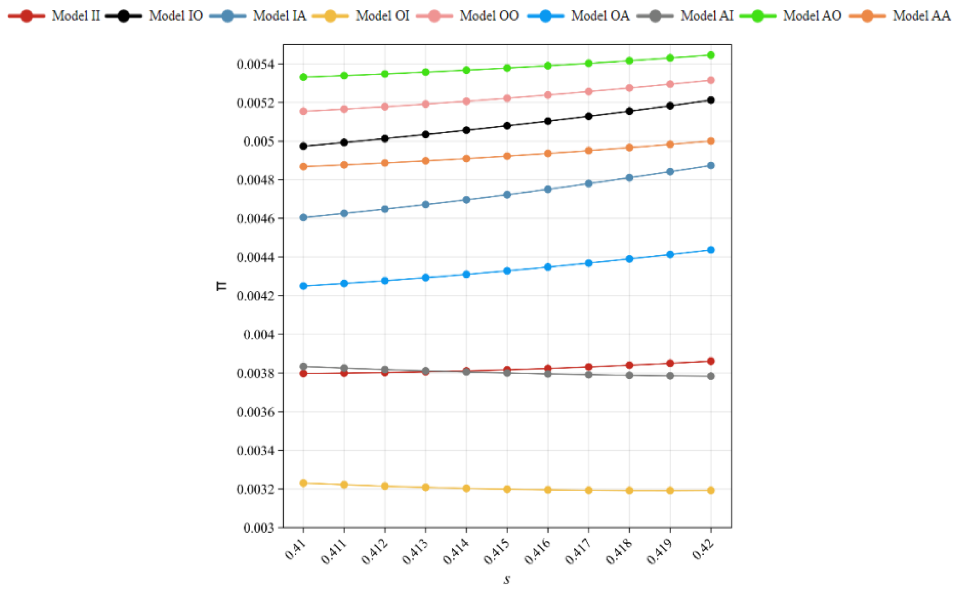
Finally, we examine the high-competition, low-discount scenario, characterized by intense market competition $(\beta =0.8)$ coupled with minimal cost advantages for remanufactured products $(\delta =0.8)$. This challenging configuration represents an industrial environment where strong competitive pressures coincide with limited economic incentives for remanufacturing—the narrow cost differential between new and remanufactured products $(s\in [0.17,0.18\left]\right)$ creates particularly complex strategic dilemmas for CLSC management, as firms must contend with fierce market rivalry while operating within constrained opportunities for cost savings through remanufacturing activities.

Corollary 9.

When in a market with high-competition and low-discounts, with the increase of unit costs, the optimal decision shifts from the authorized remanufacturing model to the outsourcing remanufacturing model.

(1) $s\in [0.17,0.173)$, take $s=0.171$, the profits of the CLSC remanufacturing model are as follows

Table 35. When $s=0.171$, remanufacturing modes profit.

CLSC1	CLSC2
	I Model	O Model	A Model
I model	(0.00315, 0.00315)	(0.004776, 0.002778)	(0.004242, 0.003182)
O model	(0.002778, 0.004776)	(0.005203, 0.005203)	(0.004317, 0.005332)
A model	(0.003182, 0.004242)	(0.005332, 0.004317)	(0.004676, 0.004676)

:

(2) Take $s=0.173$, the profits of the CLSC remanufacturing model are as follows

Table 36. When $s=0.173$, remanufacturing modes profit.

CLSC1	CLSC2
	I Model	O Model	A Model
I model	(0.003173, 0.003173)	(0.004823, 0.002786)	(0.0043, 0.003175)
O model	(0.002786, 0.004823)	(0.005243, 0.005243)	(0.004368, 0.005438)
A model	(0.003175, 0.0043)	(0.005438, 0.004368)	(0.004696, 0.004696)

:

(3) $s\in (0.173,0.179)$, take $s=0.177$, the profits of the CLSC remanufacturing model are as follows

Table 37. When $s=0.177$, remanufacturing modes profit.

CLSC1	CLSC2
	I Model	O Model	A Model
I model	(0.003232, 0.003232)	(0.004927, 0.002827)	(0.00443, 0.00317)
O model	(0.002827, 0.004927)	(0.005343, 0.005343)	(0.004496, 0.005386)
A model	(0.00317, 0.00443)	(0.005386, 0.004496)	(0.004747, 0.004747)

:

(4) Take $s=0.179$, the profits of the CLSC remanufacturing model are as follows

Table 38. When $s=0.179$, remanufacturing modes profit.

CLSC1	CLSC2
	I Model	O Model	A Model
I model	(0.003269, 0.003269)	(0.004985, 0.002859)	(0.004503, 0.003172)
O model	(0.002859, 0.004985)	(0.005403, 0.005403)	(0.004573, 0.005408)
A model	(0.003172, 0.004503)	(0.005408, 0.004573)	(0.004777, 0.004777)

:

(5) $s\in (0.179,0.18]$, take $s=0.18$, the profits of the CLSC remanufacturing model are as follows

Table 39. When $s=0.18$, remanufacturing modes profit.

CLSC1	CLSC2
	I Model	O Model	A Model
I model	(0.003288, 0.003288)	(0.005016, 0.002878)	(0.004541, 0.003174)
O model	(0.002878, 0.005016)	(0.005436, 0.005436)	(0.004614, 0.005421)
A model	(0.003174, 0.004541)	(0.005421, 0.004614)	(0.004794, 0.004794)

:

On the basis of Figure 10, the low-discount boosts the profit margins on remanufactured products, and as savings increase, this is offset by the OEM’s resistance to remanufactured products in a high-competition scenario, making all three strategies potentially optimal decisions possible.

6. Discussion

In this paper, we explored the optimal decision of remanufacturing mode for CLSCs in competitive markets. At the same time, we explored the effects of competitive intensity and remanufactured products’ discount on the decision. By developing Stackelberg game models, applying numerical analysis and Nash equilibrium analysis, we draw the following conclusions:

First, in competitive markets, OEMs predominantly adopt outsourced or authorized remanufacturing rather than independent remanufacturing. This strategic preference is evident in the automotive sector, where companies like Ford and Land Rover routinely collaborate with Third-Party Remanufacturers (TPRs) [6]. The competitive pressure creates an environment where maintaining market share through partnerships becomes more advantageous than pursuing solo remanufacturing operations. Second, the analysis demonstrates that unit savings in remanufacturing systems are primarily determined by the discounts of remanufacturing products and exhibit an inverse relationship with product discount levels. This relationship manifests clearly in Apple’s refurbished electronics operations, where products with lower discounts of remanufacturing products achieve superior quality standards but simultaneously experience reduced unit savings due to elevated production expenditures [52]. Third, competitive markets frequently drive firms toward similar remanufacturing strategies, as demonstrated by the parallel approaches of HP and Canon in the printer industry [53,54]. These conclusions suggest that successful implementation requires careful consideration of competitive positioning, strategic partnerships with TPRs, and adaptable pricing strategies. The findings provide valuable guidance for industries transitioning to circular business models while facing market competition and evolving regulatory requirements.

This study contributes to the understanding of remanufacturing strategies in competitive markets, but several important limitations should be acknowledged. The static nature of our analysis, while providing clear theoretical insights, does not capture the dynamic evolution of competition over time, where firms may adapt their strategies in response to market changes. Our assumption of homogeneous competition, where competing products share identical production costs and unit savings, represents another simplification that may not hold in practice, as firms often operate with varying cost structures and remanufacturing efficiencies. These limitations suggest several promising directions for future research. First, developing dynamic game models could provide insights into how competition evolves over multiple periods. Second, incorporating heterogeneous cost structures would allow examination of how asymmetries in production efficiencies impact strategic choices. Third, empirical validation through case studies of actual remanufacturing markets could help bridge the gap between theoretical predictions and real-world outcomes. Addressing these limitations would enhance the model’s applicability while maintaining its analytical rigor.Future research could productively examine how these dynamics vary across different industrial sectors and regulatory environments.

References

1. Liu, C.; Meng, X.; Liu, C.; Liu, Z. Carbon footprint-based optimization method for remanufacturing machining paths. Int. J. Adv. Manuf. Technol. 2023, 124, 3391–3406. [Google Scholar] [CrossRef]
2. Qiao, H.; Su, Q. Distribution channel and licensing strategy choice considering consumer online reviews in a closed-loop supply chain. Transp. Res. Part E Logist. Transp. Rev. 2021, 151, 102338. [Google Scholar]
3. Zhang, Y.; He, Y.; Yue, J.; Gou, Q. Pricing decisions for a supply chain with refurbished products. Int. J. Prod. Res. 2019, 57, 2867–2900. [Google Scholar]
4. How to Get Rid of Old Shoes Sustainably. Available online: https://www.nike.com/a/recycle-old-shoes? (accessed on 23 April 2024).
5. Here’s Ikea’s New Solution for Selling Gently Used Furnishings. Available online: https://www.furnituretoday.com/retailers/heres-ikeas-new-solution-for-selling-gently-used-furnishings/ (accessed on 6 April 2023).
6. Zhang, F.; Chen, H. Recycling or Remarketing: Optimal Strategies for Outsourcing Remanufacturing. Open J. Soc. Sci. 2020, 8, 497–506. [Google Scholar]
7. Fang, C.; Fan, S.; Qiu, Y. The choice of remanufacturing strategy for the OEM with third-party remanufacturers’ advantages. Comput. Ind. Eng. 2023, 176, 108973. [Google Scholar]
8. Yan, W.; Chai, J.; Qian, Z.; Tsai, S.B.; Chen, H.; Xiong, Y. Operational Decisions on Remanufacturing Outsourcing Involved with Corporate Environmental and Social Responsibility—A Sustainable Perspective. Sustainability 2018, 10, 1132. [Google Scholar] [CrossRef]
9. Zhao, Y.; Zhou, H.; Wang, Y. Outsourcing remanufacturing and collecting strategies analysis with information asymmetry. Comput. Ind. Eng. 2021, 160, 107561. [Google Scholar]
10. Zhou, Q.; Meng, C.; Yuen, K.F.; Sheu, J.B. Remanufacturing authorization strategy for an original equipment manufacturer-contract manufacturer supply chain: Cooperation or competition? Int. J. Prod. Econ. 2021, 240, 108238. [Google Scholar]
11. Liu, L.; Pang, C.; Hong, X. Patented product remanufacturing and technology licensing in a closed-loop supply chain. Comput. Ind. Eng. 2022, 172, 108634. [Google Scholar]
12. Huang, Y.; Wang, Z. Information sharing in a closed-loop supply chain with learning effect and technology licensing. J. Clean. Prod. 2020, 271, 122544. [Google Scholar]
13. Mutha, A.; Bansal, S.; Guide, V.D.R. Selling assortments of used products to third-party remanufacturers. Prod. Oper. Manag. 2019, 28, 1792–1817. [Google Scholar] [CrossRef]
14. Zou, Z.; Wang, J.; Deng, G.; Chen, H. Third-party remanufacturing mode selection: Outsourcing or authorization? Transp. Res. Part E Logist. Transp. Rev. 2016, 87, 1–19. [Google Scholar] [CrossRef]
15. Huang, Y.; Zheng, B.; Wang, Z. Supplier–remanufacturing and manufacturer–remanufacturing in a closed-loop supply chain with remanufacturing cost disruptions. Ann. Oper. Res. 2023, 324, 61–92. [Google Scholar] [CrossRef]
16. Feng, D.; Shen, C.; Pei, Z. Production decisions of a closed-loop supply chain considering remanufacturing and refurbishing under government subsidy. Sustain. Prod. Consum. 2021, 27, 2058–2074. [Google Scholar] [CrossRef]
17. Zhou, Y.; Liu, X.; Wong, K. Remanufacturing policies options for a closed-loop supply chain network. Sustainability 2021, 13, 6640. [Google Scholar] [CrossRef]
18. Li, W.; Sun, H.; Dong, H.; Gan, Y.; Koh, L. Outsourcing decision-making in global remanufacturing supply chains: The impact of tax and tariff regulations. Eur. J. Oper. Res. 2023, 304, 997–1010. [Google Scholar] [CrossRef]
19. Ma, P.; Li, M. Operational and financing decisions of original equipment manufacturers under third-party remanufacturing modes. Comput. Ind. Eng. 2023, 183, 109508. [Google Scholar] [CrossRef]
20. Gao, N.; Qu, L.; Jiang, Y.; Hou, J. Game Models for Ordering and Channel Decisions of New and Differentiated Remanufactured Products in a Closed-Loop Supply Chain with Sales Efforts. Systems 2024, 12, 67. [Google Scholar] [CrossRef]
21. Duan, W.; Cao, H.; Xu, D. Research on the Impact of New Parts Price Increase on the Stability of Closed-Loop Supply Chain. Sustainability 2023, 15, 12587. [Google Scholar] [CrossRef]
22. Liu, L.; Wang, L.; Huang, T.; Pang, J. The Differential Game of a Closed-Loop Supply Chain with Manufacturer Competition Considering Goodwill. Mathematics 2022, 10, 1795. [Google Scholar] [CrossRef]
23. Xu, H.; Gao, K.; Chi, Y.; Chen, Y.; Peng, R. Interactive Impacts of Overconfidence and Competitive Preference on Closed-Loop Supply Chain Performance. Mathematics 2022, 10, 4334. [Google Scholar] [CrossRef]
24. Zhao, L.; Mu, Z. Channel Strategies for the Two-Period Closed-Loop Supply Chain with E-Commerce. Mathematics 2021, 9, 1271. [Google Scholar] [CrossRef]
25. Fargetta, G.; Scrimali, L.R.M. A sustainable dynamic closed-loop supply chain network equilibrium for collectibles markets. Comput. Manag. Sci. 2023, 20, 19. [Google Scholar]
26. Zhou, F.; Chen, T.; Tiwari, S.; Si, D.; Pratap, S.; Mahto, R.V. Pricing and Quality Improvement Decisions in the End-of-Life Vehicle Closed-Loop Supply Chain Considering Collection Quality. IEEE Trans. Eng. Manag. 2024, 71, 4231–4245. [Google Scholar]
27. Li, P.; Xu, S.; Han, J. Research on the Complementarity Model of Closed-Loop Supply Chain Network Equilibrium with Environmental Indicators. Oper. Res. Manag. Sci. 2021, 30, 38–45. [Google Scholar]
28. Zhao, J.; Qu, P.; Zhou, Y. Equilibrium of a closed-loop supply chain network considering cost information asymmetry. J. Syst. Eng. 2022, 37, 749–765. [Google Scholar]
29. Gu, Y.; Xue, M.; Zhao, M.; Long, Y. Optimal Government Subsidy Decision and Its Impact on Sustainable Development of a Closed-Loop Supply Chain. Systems 2023, 11, 378. [Google Scholar] [CrossRef]
30. Wang, W.; Guan, J.; Zhang, M.; Qi, J.; Lv, J.; Huang, G. Reward-Penalty Mechanism or Subsidy Mechanism: A Closed-Loop Supply Chain Perspective. Mathematics 2022, 10, 2058. [Google Scholar] [CrossRef]
31. Cheng, P.; Zhang, G.; Sun, H. The Sustainable Supply Chain Network Competition Based on Non-Cooperative Equilibrium under Carbon Emission Permits. Mathematics 2022, 10, 1364. [Google Scholar] [CrossRef]
32. Taleizadeh, A.A.; Moshtagh, M.S.; Moon, I. Optimal decisions of price, quality, effort level and return policy in a three-level closed-loop supply chain based on different game theory approaches. Eur. J. Ind. Eng. 2017, 11, 486–525. [Google Scholar] [CrossRef]
33. Pal, B.; Guin, S.; Chaudhuri, K. Pricing and quality competition between two substitute products in a closed-loop supply chain. Int. J. Syst. Sci. Oper. Logist. 2023, 10, 2259294. [Google Scholar]
34. Wang, W.; Fan, L.; Ma, P.; Zhang, P.; Lu, Z. Reward-penalty mechanism in a closed-loop supply chain with sequential manufacturers’ price competition. J. Clean. Prod. 2017, 168, 118–130. [Google Scholar]
35. Doustmohammadi, N.; Babazadeh, R. Design of closed loop supply chain of wood plastic composite industry. J. Environ. Inform. 2020, 35, 94–102. [Google Scholar]
36. Zhang, C.; Ren, M. Closed-loop supply chain coordination strategy for the remanufacture of patented products under competitive demand. Appl. Math. Model. 2016, 40, 6243–6255. [Google Scholar]
37. Wei, J.; Chen, W.; Liu, G. How manufacturer’s integration strategies affect closed-loop supply chain performance. Int. J. Prod. Res. 2021, 59, 4287–4305. [Google Scholar]
38. Yu, Z.; Lin, Y.; Wang, Y.; Goh, M. Closed-loop supply chain coalitional cooperation and coordination under differentiated carbon tax regulation. J. Clean. Prod. 2023, 392, 136239. [Google Scholar]
39. Zhong, L.; Nie, J.; Lim, M.; Xia, S. Agency or Self-Run: The effect of consumer green education on recyclers’ distribution channel choice under platform economy. Int. J. Logist. Res. Appl. 2022, 25, 814–836. [Google Scholar]
40. Luo, R.; Zhou, L.; Song, Y.; Fan, T. Evaluating the impact of carbon tax policy on manufacturing and remanufacturing decisions in a closed-loop supply chain. Int. J. Prod. Econ. 2022, 245, 108408. [Google Scholar] [CrossRef]
41. Zhang, Y.; Chen, W.; Mi, Y. Third-party remanufacturing mode selection for competitive closed-loop supply chain based on evolutionary game theory. J. Clean. Prod. 2020, 263, 121305. [Google Scholar]
42. Li, X.; He, J. Mechanism of the green supply chain profit of building materials considering the duopoly competition model and consumer green preference. Int. J. Syst. Sci. Oper. Logist. 2024, 11, 2311283. [Google Scholar]
43. Li, W.; Jin, M.; Galbreth, M.R. Should original equipment manufacturers authorize third-party remanufacturers? Eur. J. Oper. Res. 2024, 314, 1013–1028. [Google Scholar] [CrossRef]
44. Toyota, V.S. Honda—9 Important Differences (Before Buying). Available online: https://motorandwheels.com/differences-between-toyota-honda/ (accessed on 23 October 2023).
45. Song, L.; Liu, S.; Yao, F.; Xing, Y. Collection and Coordination Strategies in a Dual-Channel Closed-Loop Supply Chain Under Manufacturer Diseconomies of Scale. IEEE Access 2021, 9, 113377–113392. [Google Scholar] [CrossRef]
46. Lin, G.; Xiong, X.; Li, Y.; Zhu, X. Sales Mode Selection Strategic Analysis for Manufacturers on E-Commerce Platforms under Multi-Channel Competition. Systems 2022, 10, 234. [Google Scholar] [CrossRef]
47. Zhang, H.; Zhang, Y.; Li, P.; Zheng, H.; Li, Z. Low-carbon production or not? Co-opetition supply chain manufacturers’ production strategy under carbon cap-and-trade policy. In Environment, Development and Sustainability; Springer: Berlin/Heidelberg, Germany, 2022. [Google Scholar]
48. Patek Philippe VS Rolex Watches. Available online: https://www.prestigetime.com/blog/patek-philippe-vs-rolex.html/ (accessed on 15 March 2025).
49. Alternator Recycling: Conserving Resources, Reducing Waste. Available online: https://automotiveitnews.org/alternator-recycling (accessed on 21 May 2024).
50. Refurbished vs New: A Comprehensive Cost-Benefit Analysis Across Popular Tech Categories. Available online: https://www.officiallyrefurbished.com/blog/refurbished-vs-new-cost-benefit-analysis (accessed on 12 August 2024).
51. The Cisco Refresh Difference. Available online: https://www.cisco.com/c/en/us/products/remanufactured/refresh-difference.html (accessed on 25 March 2025).
52. How Used Products Can Unlock New Markets: Lessons from Apple’s Refurbished iPhones. Available online: https://www.library.hbs.edu/working-knowledge/how-used-products-can-unlock-new-markets-lessons-from-apples-refurbished-iphones (accessed on 12 March 2024).
53. Canon Honoured for Its Initiatives to Expand Remanufacturing of Multifunction Devices. Available online: https://www.therecycler.com/posts/canon-honoured-for-its-initiatives-to-expand-remanufacturing-of-multifunction-devices/ (accessed on 25 October 2024).
54. Wu, J.; Zhang, L.; Shen, X. Outsourcing or Authorizing? Optimal Options for Third-Party Remanufacturing Modes with Green Consumerism. Sustainability 2024, 16, 1914. [Google Scholar] [CrossRef]
Figure 1. Model structure: (a) Model II (b) Model IO (c) Model IA (d) Model OO (e) Model OA (f) Model AA.
Systems 13 00257 g001
Figure 2. Profits of CLSC under nine strategies.
Systems 13 00257 g002
Figure 3. Profits of CLSC under nine strategies.
Systems 13 00257 g003
Figure 4. Profits of CLSC under nine strategies.
Systems 13 00257 g004
Figure 5. Profits of CLSC under nine strategies.
Systems 13 00257 g005
Figure 6. Profits of CLSC under nine strategies.
Systems 13 00257 g006
Figure 7. Profits of CLSC under nine strategies.
Systems 13 00257 g007
Figure 8. Profits of CLSC under nine strategies.
Systems 13 00257 g008
Figure 9. Profits of CLSC under nine strategies.
Systems 13 00257 g009
Figure 10. Profits of CLSC under nine strategies.
Systems 13 00257 g010