Abstract
(1) Background: The reliability of port equipment is of significant interest to industry stakeholders due to the economic and logistical factors governing the operation of maritime container terminals. Failures of key equipment like quay cranes can halt operations or cause economically significant delays. (2) Methods: The impact assessment of these disruptive events is conducted through terminal activity modeling and discrete-event simulation of internal processes. The system’s steady-state or transient condition, induced by disruptive events, is statistically assessed within a set of scenarios proposed by the authors. (3) Results: The Heidelberg–Welch and Geweke tests enabled the evaluation of steady-state and transient conditions within the modeled system, which was affected by the reduced reliability of container-handling equipment. (4) Conclusions: The research findings confirmed the usefulness of modeling and simulation in assessing the impact of equipment reliability on maritime container terminal operations. If the magnitude of the disruptive event exceeds the terminal’s absorption capacity, the system may become blocked or remain in a transient state without the ability to recover. This underscores the necessity of analyzing the reliability of critical handling equipment and implementing corrective maintenance actions when required.
1. Introduction
Maritime container terminals are a crucial component of global logistics chains, serving as key hubs connecting maritime transport with land-based networks. The movement of goods across countries and continents is facilitated by high-capacity container ships. By using maritime container terminals, economic connections between geographically distant nations are strengthened, contributing to global economic growth and development. According to UNCTAD, containerized transport remains essential in 2023, with an estimated volume of transported goods nearing 2000 million tons. The number of loading units has also remained stable at approximately 164 million twenty-foot equivalent units (TEUs) [1]. These figures underscore the operational pressure faced by maritime container terminals providing uninterrupted service while mitigating the impact of disruptive events. Such events include natural phenomena (e.g., storms, strong winds, snow) as well as failures in handling, storage, and transport equipment within the terminal. The research presented in this study focuses on evaluating the impact of the latter category on terminal operations. The terminal is modeled as a dynamic system characterized by multiple operational states, which arise from either full-capacity or under-capacity operation resulting from disruptive events, such as the failure of a quay crane. Thus, the system could be in a stationary or non-stationary state.
Efficient container terminal operations are a critical goal for terminal management. The main objective of the research is achieved by designing a layout that meets the terminal’s specific operational requirements. The layout must effectively integrate various modes of transport (maritime vessels, trucks, trains), handling and storage equipment, and designated storage areas within the terminal [2]. The proper functioning of handling, storage, and transport equipment is analyzed using reliability functions and performance indicators. The occurrence of a disruptive event can significantly impact the terminal’s economic efficiency [3]. Equipment failures, particularly those affecting container-handling machinery, can lead to substantial operational disruptions. While terminal operational reserves may help absorb and mitigate these disruptions within an acceptable timeframe, in certain cases, the magnitude of the disturbance results in severe degradation of service quality parameters, ultimately affecting the terminal’s economic productivity. Research in this field primarily focuses on modeling the activities of the terminal and evaluating key service quality parameters, such as waiting times, the number of handling operations and storage area optimization. However, a notable gap exists in analyzing the impact of handling equipment failures resulting from reduced reliability. The practical implications of handling equipment reliability for maritime container terminal administrators can be highly diverse. The strategic and operational analysis conducted by these administrators must consider equipment reliability, its utilization level within terminal processes, and the costs associated with its acquisition, operation, and potential failures when making investment decisions. In many cases, maritime container terminals operate within multinational corporations that strictly manage acquisition and operational costs. The occurrence of an unforeseen disruptive event is often difficult for the management of such companies to accept. However, the impact of such an event can be minimized if it primarily affects equipment with a low influence on overall terminal operations due to their availability—such as a terminal truck breakdown. Conversely, it can be a major influence if critical equipment, such as a quay crane, fails. A reduction in the handling and storage capacity at the terminal level is not easily accepted by its management. For this reason, research on system state evaluation—whether stable or transient—is of interest both from an organizational perspective and in terms of economic implications.
In this study, discrete-event modeling was employed as a methodological approach, with a practical application to a real-world container terminal in Europe. The input data for the model was collected from terminal administration and processed to ensure accurate integration into the developed simulation framework. The primary data collected included information on the arrival times of vessels at the container terminal, the technological processes occurring within the terminal, the time durations required for these processes, as well as topological aspects necessary for simulation related to terminal design. Since data collection was conducted during summer, disruptions caused by meteorological phenomena that could lead to terminal activity interruptions or restrictions on maritime vessel access to berths are not considered.
A set of scenarios was designed to assess the impact of quay crane failures over varying time periods. The data analysis enabled the identification of periods in which the modeled system operated in either a transient or steady state. Additionally, scenarios in which a return to the steady-state condition in due time is no longer possible were identified.
Building upon the previously introduced concepts and methodology, this research aims to identify the system states in response to a disruptive event. In the specific case of maritime container terminals, discrete-event modeling provides a feasible tool for evaluating operational parameters that define a system’s stable or transient state. To comprehensively present the research conducted, the article is structured as follows:
- Introduction: This section provides a descriptive overview of the challenges encountered in container terminal operations and identifies the key activities that may be disrupted by external perturbations.
- Literature Review: A critical review of existing studies in the field is conducted to identify research gaps and establish the baseline from which this study originates.
- Modeling the Equipment Reliability: This section presents the mathematical framework underlying equipment reliability assessment, system state analysis, and stationarity vectors.
- Simulation Model and System States: It details the methodology and structural components of the simulation model used as a tool for generating operation scenarios.
- Case Study: Constantza South Container Terminal: This section describes the primary data collected from a real maritime container terminal and presents the scenarios tested in the simulation model to evaluate system state transitions.
- Results and Discussion: The findings obtained through simulation are presented, with a focus on waiting times measured for each simulation entity across the seven proposed scenarios.
- Conclusions: This section summarizes the authors’ conclusions regarding the necessity and innovative aspects of the research, as well as future research directions derived from the obtained results. The identified limitations of the model are also discussed, along with potential methods to address them.
2. Literature Review
Due to its significant economic importance, the maritime container terminal has been the subject of extensive research, which has addressed various aspects, including strategic development, marine pollution, modeling of both terminal operations and related activities, as well as the evaluation of terminal reliability as a complex system. According to Steenken et al., three decision-making levels can be identified (strategic, operative planning, and real-time control) [4].
From a strategic perspective, research has been conducted both at the level of logistics chain [5,6] and through comparative analyses of land-use and terminal localization [7]. Some studies focus on the specific aspects of developing new terminals [8], while others assess the factors influencing the competitiveness of maritime container ports [9]. A specialized area of research within this strategic framework examines the impact of mooring of ultra-large container vessels on port infrastructure. The increasing deployment of high-capacity vessels has significant implications for port infrastructure development [10]. Simulation-based research can also be used to identify strategies for port infrastructure development. This approach enables the identification of opportunities for port expansion to become local or regional hubs [11].
Another key research direction addresses the environmental impact of maritime container terminal operations. Advanced methodologies, such as the Automatic Identification System (AIS), are employed to decode vessel data and estimate ship emissions. These analyses incorporate information on ship technical specifications and operational characteristics [12]. Additionally, research on pollution examines the technical aspects of data transmission from monitoring systems [13,14]. Indicators such as the Ship Carbon Intensity, proposed by the International Maritime Organization, play a crucial role in assessing the environmental impact of vessel scheduling for cargo handling activities [14]. In this context, optimization processes in the terminal may inadvertently lead to negative environmental consequences. However, maritime terminals are also evaluated in terms of sustainability strategies. For instance, implementing automated mooring and unmooring technologies can reduce greenhouse gas emissions in port operations [15]. Furthermore, reviews of environmentally friendly practices, technologies, and equipment contribute to define a “model” port concept, which could be theoretically adopted by port administrations worldwide [16,17]. In relation to port terminals, the maritime transport component and voyage attributes, such as travel speed, can affect pollutant emissions, cargo lead time, and supply chain costs [18]. Likewise, in terms of the environmental component, the choice of a specific mode of transport, such as container transport, ensures the integration of maritime terminals into the sustainable development strategy of ports [19]. The connection with terrestrial transport networks can also be evaluated from an environmental perspective, particularly in terms of emissions. Urban congestion in port cities can lead to pollution hotspots, which is why research in this area is also of significant importance [20]. Scenarios involving new technologies (electric trains, hydrogen trains) with a positive environmental impact have been studied using simulation tools. The results obtained thus enable the development of optimal strategies for their control to maximize benefits [21].
At the operational planning level, research has focused on mathematical modeing of interactions between transport modes, handling equipment, and even between multiple container terminals. Studies in this area explore ways to enhance port performance by improving knowledge of terminal operating systems [22,23,24,25,26,27,28,29,30,31,32,33,34]. One key aspect of this research involves evaluating the interaction between land transport networks and terminal operations. Metrics such as truck queue length and waiting times at terminal gates are critical for assessing service efficiency [23,24,25,26,27,28,29,30]. The event-oriented simulation method can be used to simulate road traffic in the port area for a comprehensive analysis of port logistics systems. Discrete-event modeling thus proves to be a valuable tool for evaluating these systems [27]. Discrete-event simulation (DES) models are highly versatile tools, with applications in cost–benefit analysis, predicting container arrival times at terminals and berth allocation within port terminals [28,29,30]. Findings indicate that implementing a structured truck appointment system can significantly influence drayage costs and overall efficiency [31]. Similarly, optimizing rail transport and synchronizing terminal activities with adjacent railway stations have been shown to reduce delays and increase transit capacity [32,33].
At the same operational level, research has addressed berth allocation and container relocation problems. Heuristic methods and genetic algorithms have proven to be useful in solving these challenges [34,35]. Additionally, simulation models offer advantages in terms of adaptability and time compression for scenario-based analyses [36,37].
A notable gap in existing research at this level is the analysis of the impact of disruptive events on terminal operations. Few studies have explored the diverse nature of these disruptions. One such study [38] examines the impact upon business of power outages at container terminals. In another study [39], the authors focus on resilience measurement and dynamic optimization of the container logistics supply chain under adverse events. However, the study is largely theoretical. A clear gap emerges between the well-developed theoretical concepts presented by the authors and the application of discrete-event simulation, which is essential for accurately modeing operations in a maritime container terminal. The present research aims to address this gap by analyzing the reliability of handling equipment and the consequences of equipment failures. This area of study has significant practical implications, providing valuable insights for maritime container terminal administrators in enhancing operational resilience.
3. Modeling the Equipment Reliability
3.1. The Equipment Reliability Indicators
The reliability function R(t) is calculated as a probability that the equipment will perform its intended function without failure under specified conditions for a certain period. A set of indicators is used to evaluate the dependability and consistent performance of the equipment:
- Mean Time Between Failures (MTBF): the average time between successive failures for repairable equipment.
- Mean Time To Failure (MTTF): the average time for a piece of equipment to operate before failing, applicable to non-repairable equipment.
- Failure Rate (λ(t)): the frequency at which equipment fails, expressed in failures per unit of time (t, t + Δt).
- Availability: the proportion of time that the equipment is in a functioning state. This metric is used for repairable equipment.
- Maintainability (Mean Time To Repair): the average time required to repair a piece of equipment.
Other mathematical indicators used can be:
- Failure function (F(t)): the probability that an equipment will fail during the time interval (0,t)
- The breakdown frequency of failures (f(t)): the limit of the ratio between the probability of failure in the interval (t, t + Δt) and the size of the interval
The primary relationships between these indicators are summarized in Table 1.

Table 1.
Dependences among reliability indicators [40].
For different distributions of the failure function F(t), the reliability indicators are depicted in Table 2.
Table 2.
Reliability indicators [40].
3.2. The Transient Period Toward Stationarity
Following a disruption of the container handling process (e.g., equipment breakdown, accidents), the system enters a non-stationary phase, where ships and containers are queuing, and increased waiting times are counted. Once the disruption ends, if the arrival process is stationary, the system moves asymptotically toward a steady state characterized by three conditions: (i) constant mean (the mean of the time series is constant over time), (ii) constant variance (the variance of the time series is constant over time), and (iii) constant autocovariance (the covariance between observations at any two points in time depends only on the time lag between them). Heavily loaded systems tend more slowly to a stationary state. Burn-in data refers to the portion of discarded observations so that the effect of initial values on the posterior sequence is minimized. A variety of methods have been proposed to circumvent the non-stationarity and the autocorrelation among collected observations and to evaluate the transient phase duration to steady state (burn-in data) [41,42].
Based on the remark that removing the initial transient data from a given sequence of observations has the remaining sequence behaving as a stochastic stationary process, Schruben [43] and Schruben et al. [34] developed a test to identify the transient phase. Given the output series of observations , the test is based on the high sensitivity of the sequence of partial sums:
where k = 0, 1, …, , and are means over n and k first observations. Assuming under null hypothesis that the output series is stationary, the standardized sequence of partial sums, namely,
converges to a Brownian bridge process with zero mean and variance equal to 1 as n→∞.
Using spectral analysis of variance and the findings of Schruben [33] and Schruben et al. [44] on detecting initial transients using Brownian bridge theory, Heidelberg and Welch [45] proposed a convergence test consisting of two parts:
- Calculation of the Cramér–von Mises (CVM) statistic on the whole sequence and test the null hypothesis that it comes from a stationary distribution. If the null hypothesis is rejected, then discard the first 10% of the sequence and repeat the stationarity test. If the null hypothesis is rejected, then discard the next 10% and calculate the statistical test. Repeat until the null hypothesis is accepted or 50% of the initial sequence is discarded. If the test still rejects the null hypothesis, then the observation sequence fails the test and needs to be run longer.
- If the sequence passes the first part of the diagnostic, then the part of the sequence that was not discarded from the initial one is used to compute the half-width of the mean. Half-width of this interval is compared with the estimate of the mean. If the ratio between the half-width and the mean is lower than ϵ, the half-width test is passed. Otherwise, the length of the sample is deemed not long enough to estimate the mean with sufficient accuracy and more observations must be added.
Heidelberg and Welch [45] suggest increasing the run length by a factor I > 1.5, each time, so that the estimate has the same, reasonably large proportion of new data.
Geweke [46] proposed a convergence diagnostic based on a test for equality of the means of the first and last part of a chain. Two sequences of the observation data are used and , where , being let the size of the second sequence. The two sequences do not overlap, so . The means of the two sequences are and . Being let and denote the consistent spectral density at zero frequency for the two sequences. If the initial sequence is stationary, then the statistics
converges to standard normal distribution N(0,1) as . The Geweke test is a two-tailed test with the null hypothesis of equal means of the two sequences. A large absolute value of Z indicates rejection of the null hypothesis.
To test the stationarity of the ship’s waiting time and to compute the burn-in numbers of observed data, the following steps are taken:
- To use the Heidelberg–Welch test to prove that the initial ship’s waiting time sequence is stationary and compute the confidence interval of the ship’s waiting time mean. If the test fails, a larger amount of data are required, and the first step is repeated.
- To use the Geweke test for as the author suggested. The first half of the initial ship’s data sequence is divided into segments, then Geweke’s Z-score is repeatedly calculated. The first Z-score is calculated with all iterations in the chain, the second after discarding the first ship’s wait time data segment, the third after discarding the first two segments, and so on. The last Z-score is calculated using only the samples in the second half of the ship’s wait time data sequence. The analysis of the sequence of Geweke’s Z-score indicates the burn-in ship’s data, where the Z-statistic is outside the 95% confidence interval. Following the burn-in point, the stationarity of the ship’s waiting time is achieved.
4. Simulation Model and System States
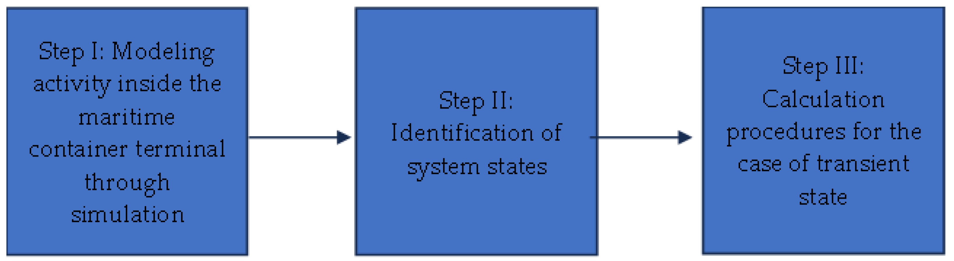
To assess the impact of the equipment reliability on operations within a maritime container terminal, the first step is to model terminal activities using a simulation model. At this stage, key activities that significantly influence the quality of services provided by the terminal are identified. In the case of a maritime terminal, quay cranes are among the most critical components due to their essential role in loading and unloading containers from maritime vessels. The level of detail in each individual simulation can lead to the omission of critical components of terminal operations or introduce evaluation errors by generating inconsistencies that are difficult to detect. In the case of the simulation tool used in the paper’s case study, the authors have identified the significant impact of quay crane operations on overall terminal performance. Specifically, the handling capacity of containers both on the vessel and at the quay can act as a limiting factor for the entire maritime terminal’s throughput.
The second stage of the research involves identifying the various states in which quay cranes can operate and modeling their reliability using a suitable distribution function. The system’s stationary state may transition into a transient state and vice versa, depending on equipment reliability and operational conditions.
Finally, specific computational procedures are applied to evaluate the duration for which the system remains in a transient state, during which the operating parameters of the container terminal are affected. The research framework is illustrated in Figure 1.
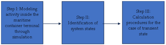
Figure 1.
The logical flow of the research—source: authors.
The topology of maritime terminals and the interdependencies between container handling and storage processes facilitate their modeling through queuing theory. The discrete-event simulation modeling is preferred due to its suitability for capturing complex system dynamics. The effectiveness of this modeling approach has been demonstrated in previous research within the same or related fields [47,48,49]. The simulation model was developed using ARENA 12 software. Through dedicated modules, simulation entities are created, and logical processes are employed to replicate real-world operations within a maritime container terminal. Each simulation block serves a specific function, as outlined in Table 3.
Table 3.
The simulation modules for the maritime container terminal model.
To simulate the occurrence of a failure of the container handling equipment, a set of new modules are introduced into the simulation model (Table 4).
Table 4.
The simulation modules for controlling equipment failure.
The modeled system states and disruptive events generated by the failure of a container handling equipment on the quays with the help of the simulation model are drawn in Figure 2.
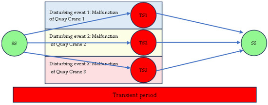
Figure 2.
The system state (SS—stationary state, TS1—transient state 1, TS2—transient state 2, TS3—transient state 3)—source: authors.
5. Study Case of Constantza South Container Terminal
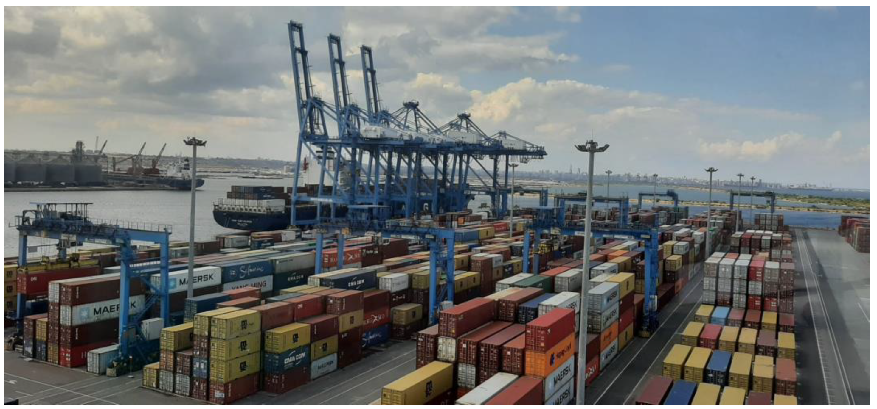
The Constantza South Container Terminal (CSCT) is the most significant container terminal in the European Union along the Black Sea. This maritime terminal is part of a global network operated by DP World. Its current capacity is approximately 1,200,000 TEU per year. Achieving and maintaining this throughput requires a precise evaluation of terminal flows and ensuring that the handling equipment has sufficient capacity to accommodate the operational demands. The most critical component of container handling—both for transferring containers from maritime vessels to land transport networks and for loading containers arriving from the port’s hinterland onto ships—is represented by quay cranes (Figure 3).

Figure 3.
The quay cranes used inside CSCT—source: authors.
The occurrence of a disruptive event in quay crane operations results in alterations to the operating parameters of the entire port. Analyzing the impact of quay crane failures is of particular interest due to their significant economic implications for port activities.
The terminal is equipped with three types of quay cranes, which are arranged in groups—five positioned on one side of the terminal and one separately. The main characteristics of these cranes are detailed in Table 5. The number of cranes utilized typically ranges from one to three, depending on factors such as the vessel’s specifications, crane availability, the number of containers, and their positioning on the vessel.
Table 5.
Main characteristics of quay cranes [50].
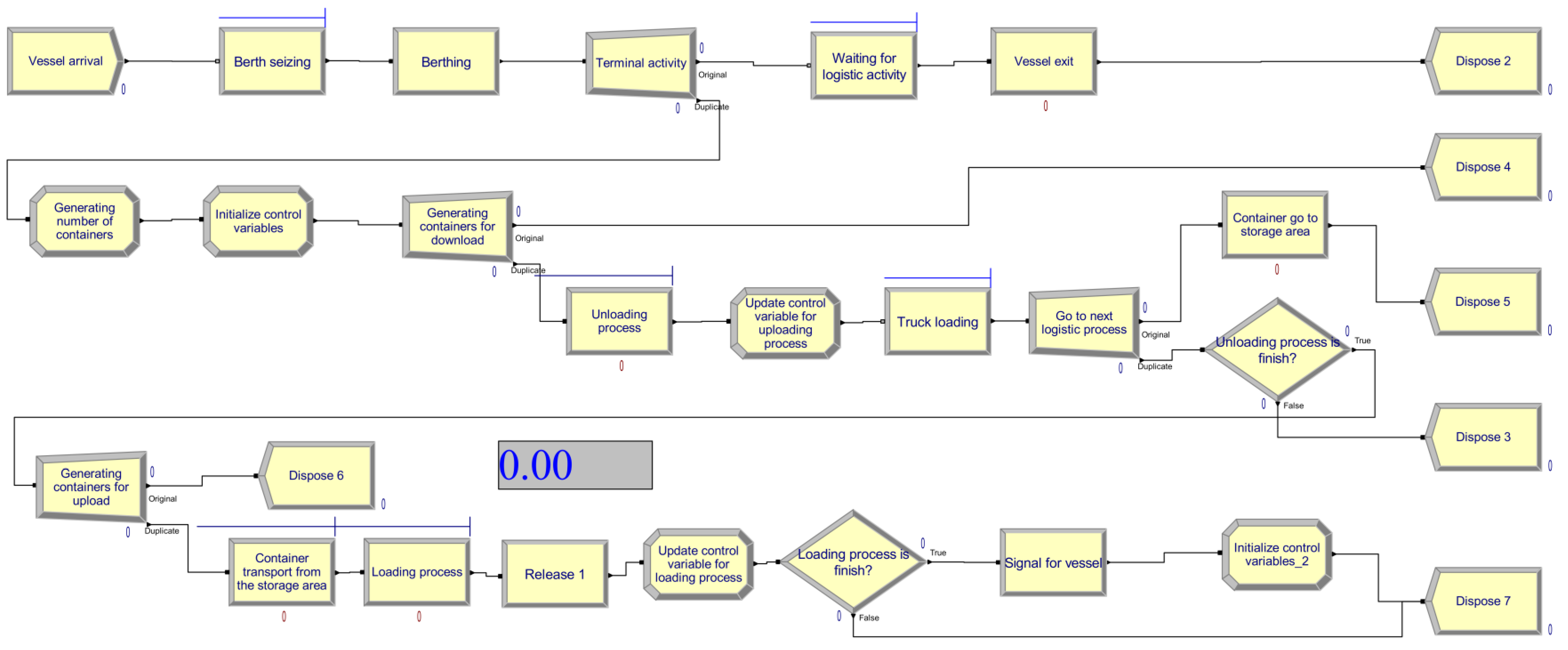
The simulation model developed in ARENA 12 is depicted in Figure 4. The simulation models the unloading and loading of containers onto ships using quay cranes. Within the terminal, these containers are further manipulated with the assistance of various types of equipment [4], including Rubber-Tired Gantries (RTG), Rail-Mounted Gantries (RMG), Empty Handlers (ECH), Reach Stackers (RS), Terminal Tractors (ITV), and Terminal Chassis (TC). However, these auxiliary equipment types were excluded from the simulation. Given their high numbers within the terminal, they provide sufficient reliability, leading the authors to deem their inclusion unnecessary for the scope of this study. The simulation model, developed using ARENA 12, is illustrated in Figure 4.
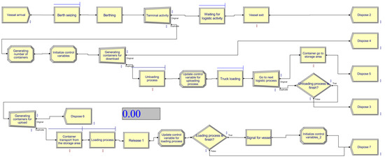
Figure 4.
The simulation model—source: authors.
Data collection was conducted over the three summer months. As a result, the dataset does not capture periods of terminal shutdowns that could have been caused by extreme weather events. However, the absence of such disruptions does not significantly impact the simulation results, as maintenance activities would also be unfeasible during these periods with potential interruption due to the terminal’s location within the maritime access zone of the port. The use of statistical tools in processing primary data is essential for developing simulation models [51]. The quality of the data input into the simulation model has a significant impact on the credibility of the results obtained. The time intervals between the loading and unloading processes of maritime vessels are represented in the graph from Figure 5.
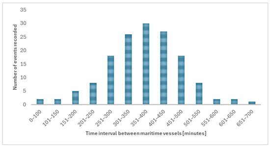
Figure 5.
Time intervals between vessel arrivals.
To represent this flow within the simulation model, the normal distribution function was selected, where the parameter μ = 390 min represents the mean (which is also the median and mode), and the parameter σ2 = 30 min denotes the variance. The arrival of sea vessels follows a schedule established by the terminal administration, which considers the time required to complete container handling operations for the preceding vessel. To accurately reflect this schedule in the simulation, a time variable was integrated. The number of containers handled per vessel is modeled using a normal distribution, with parameters estimated based on the aforementioned variable.
The input data in simulation are presented in Table 6.
Table 6.
Main attributes of simulation input data.
To study the influence of equipment reliability over the activity inside the maritime container terminal, a series of scenarios were created. The simulation parameters for each scenario are presented in Table 7. The first scenario is a base situation with all three quay cranes working.
Table 7.
The simulation scenario.
6. Results and Discussions
The simulation model was used to obtain data in all seven scenarios. The stationarity of the ships’ waiting time series for berth access is considered in analysis. For scenario S00, the ships’ waiting time series and its density are depicted in Figure 6.

Figure 6.
Ships’ waiting time series (values and density)—scenario S00.
The Heidelberg–Welch test is passed (p = 0.851) and the ships’ wait time series is stationary. The average wait time of the ships is 0.827 (h), and the quantiles are shown in Table 8.
Table 8.
Ships’ wait time quantiles.
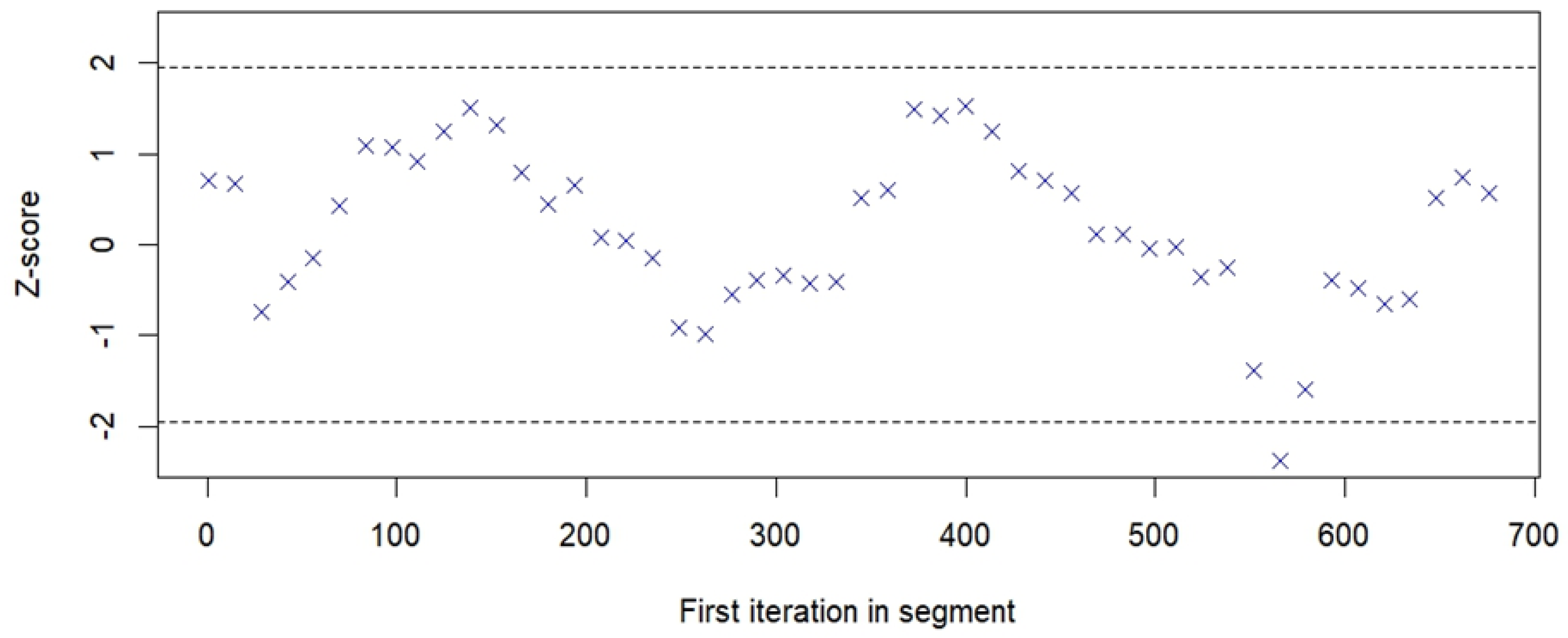
Comparing the first 10% of the series with the last half, the Geweke test statistics is 0.707, that confirms the stationarity. The plot of the z values () using the Geweke test for different fractions of the first half of the ships’ waiting time series is presented in Figure 7. All the Z-scores move between ±1.96, so the differences between the mean waiting time in the first half bins and the mean of the last half of the series are not significant.
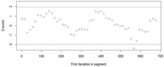
Figure 7.
Z−scores in the first half of the ships’ waiting time series (50 bins).
When the system experiences crane breakdowns, the ships’ waiting time series following the moment of the breakdown are recorded and the stationarity of the series is tested.
For different numbers of cranes out of order and various durations of the breakdown, the results are depicted in Figure 8, Figure 9, Figure 10, Figure 11, Figure 12 and Figure 13.

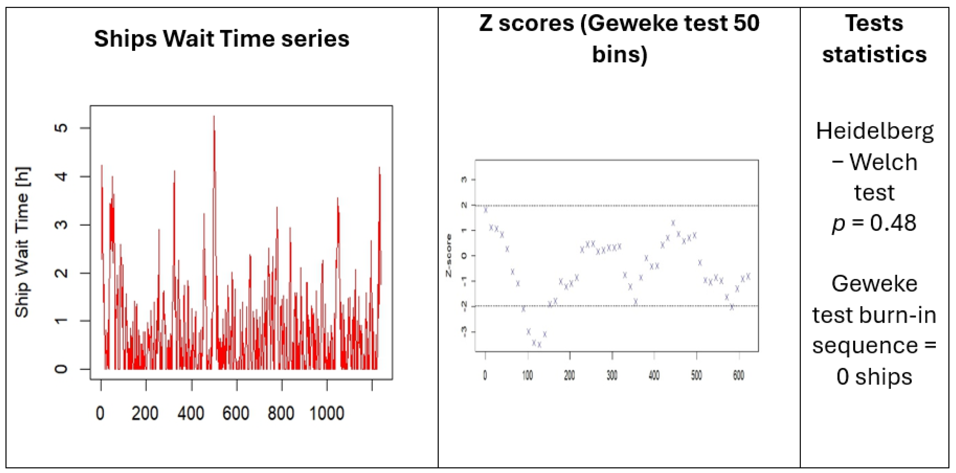
Figure 8.
Ships’ wait time series—scenario S11.
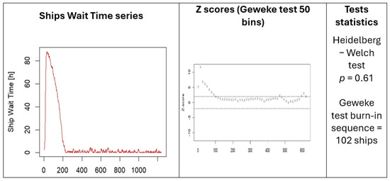
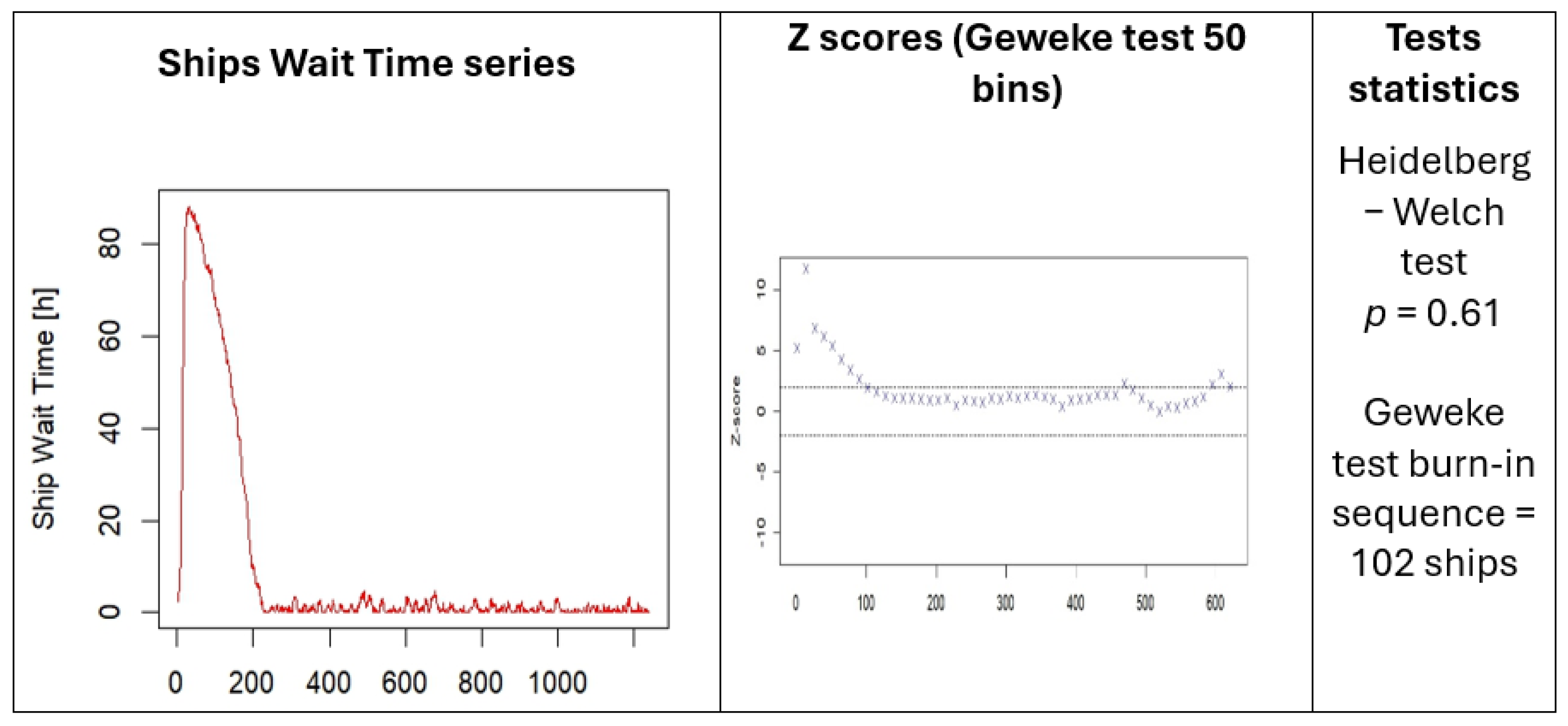
Figure 9.
Ships’ wait time series—scenario S17.
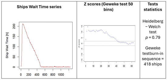
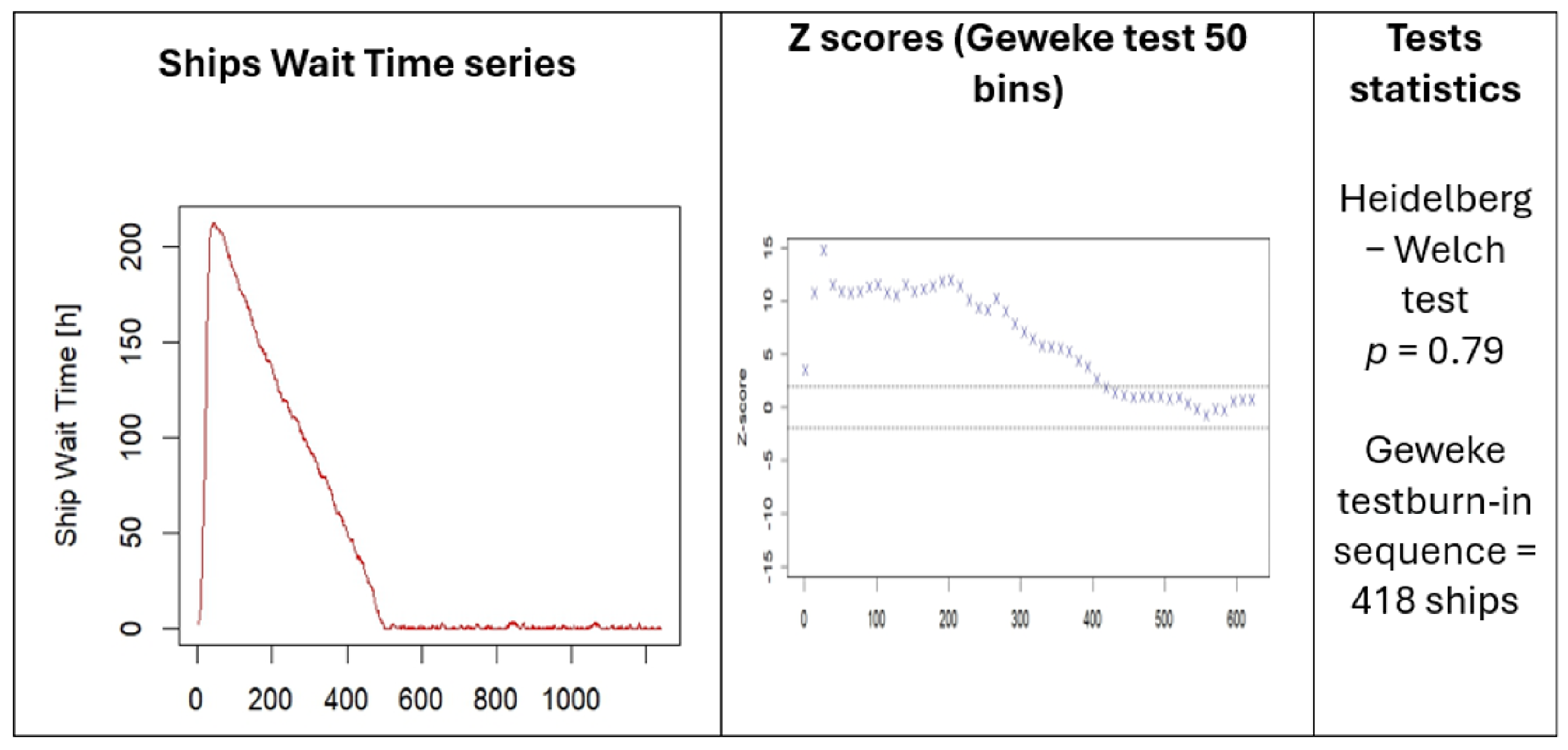
Figure 10.
Ships’ wait time series—scenario S114.

Figure 11.
Ships’ wait time series—scenario S21.
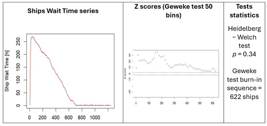
Figure 12.
Ships’ wait time series—scenario S27.
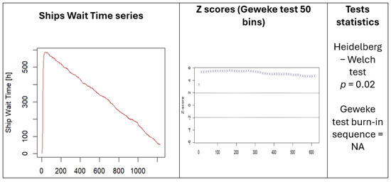
Figure 13.
Ships’ wait time series—scenario S214.
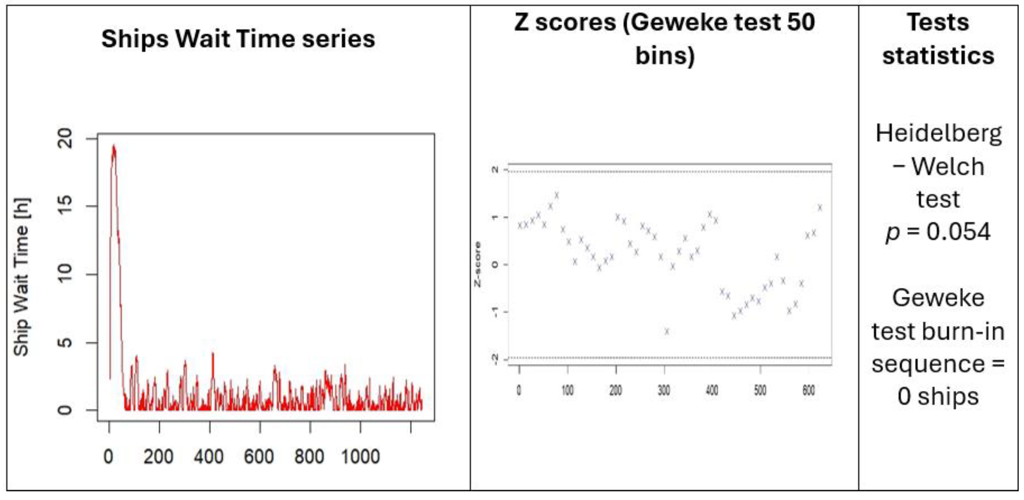
When one crane is out of order, the ships’ waiting time series is going stationary, and the Heidelberg–Welch test provides p > 0.05 for scenarios S11, S17, and S114. The z-scores in the Geweke test follows the ±1.96 interval after a burn-in sequence that depends on the breakdown duration. If the crane is stopped for 7 days, the stationarity is gained after a burn-in sequence of 102 ships, and after 418 ships when the crane is broken for 14 days.
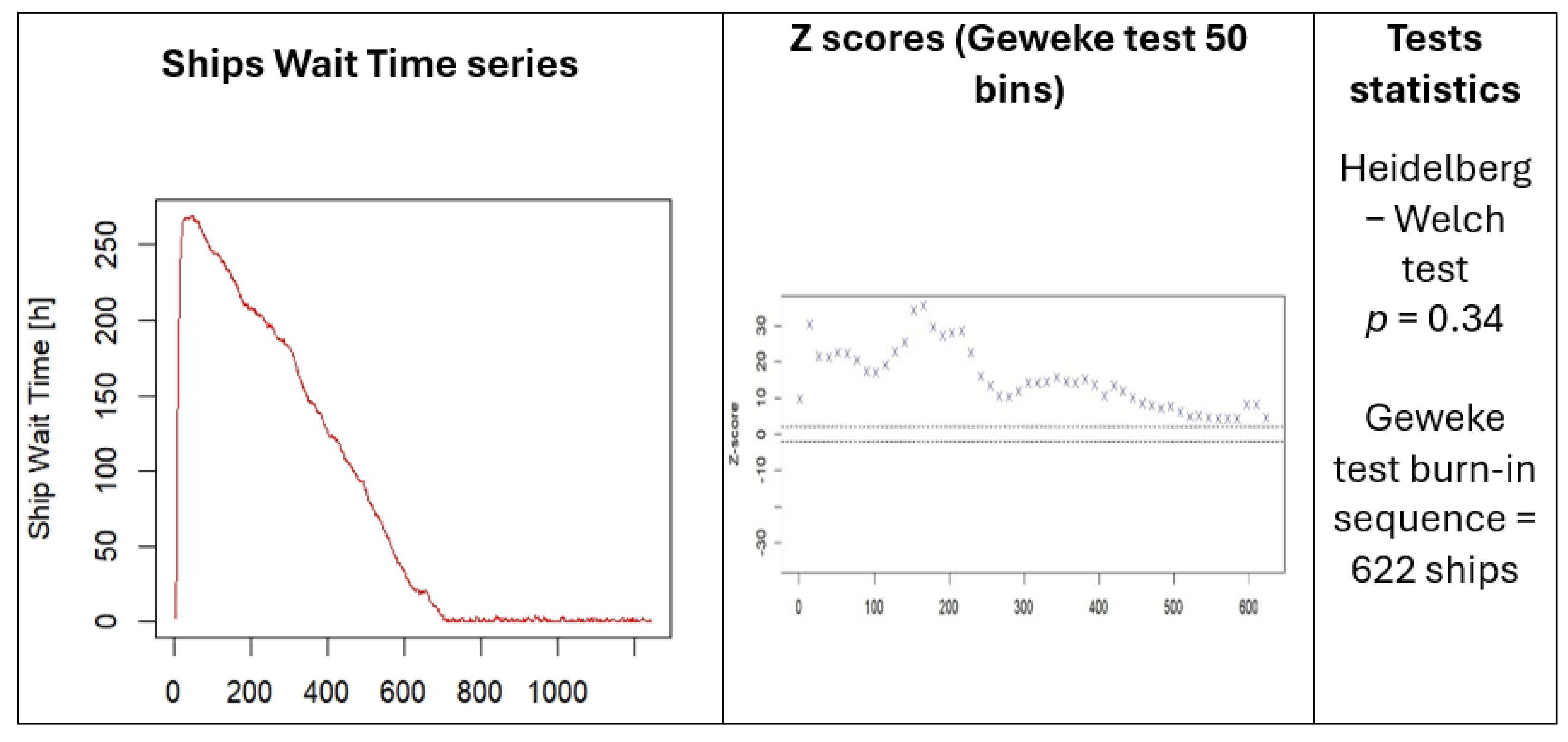
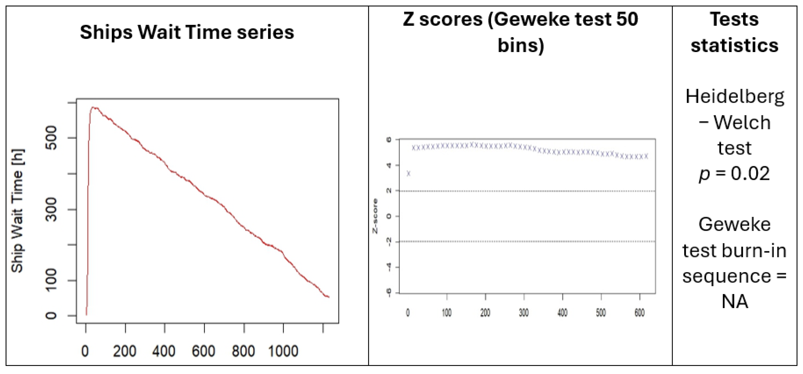
If two cranes are out of order for one day (scenario S21), the ships’ wait time series is stationary and the Geweke z-scores are in the limits of convergence. For 7 days of breakdown (scenario S27), the series becomes stationary (Heidelberg–Welch p = 0.34), but the Geweke z-scores tends to the convergence interval at the end of the series’ first half (622 ships). If the interruption of cranes is 14 days, the series is not stationary (Heidelberg–Welch p = 0.02), and the z-scores are out of the convergence interval for the provided simulation length. A longer simulation run is needed to analyze the moment when the time series becomes stationary.
The findings highlight several key implications that container terminal administrators should consider enhancing operational efficiency and resilience:
- Identification of Critical Equipment: It is essential to identify the terminal’s critical equipment, whose failure could severely disrupt operations and impact overall efficiency.
- Significance of Maintenance Strategies: Effective maintenance planning plays a crucial role in ensuring uninterrupted terminal operations, minimizing downtime, and preventing costly disruptions.
- Mitigating the Impact of Unforeseen Events: Unexpected disruptions can have significant consequences. Therefore, maintaining reserve capacity in the allocation of handling equipment is a strategic necessity to ensure operational continuity.
- Leveraging Discrete-Event Simulation Models: The use of discrete-event simulation enables cost-effective scenario testing, facilitating the identification of operational bottlenecks and critical vulnerabilities within terminal activities.
The conducted research presents a novel approach by combining discrete-event simulation with a mathematical model to evaluate the system’s transition between states. In previous studies [26,27,30,33], simulation model results have been utilized in the strategic development process of the terminal. At the same time, in [39], the focus is on evaluating the resilience and dynamic optimization of terminal operations under the influence of disruptive events. However, the integration of discrete-event modeling with a mathematical model to determine system state transitions has not been previously explored. The results obtained in this study thus become a powerful tool for port administration in selecting the maintenance plan for critical equipment, specifically quay cranes.
7. Conclusions
The study of the impact of equipment failures in container terminal operations holds particular interest due to its significant economic implications. Even though the probability of failure for a critical piece of equipment—such as one or more quay cranes—is low, the impact of such an event can be substantial.
A simulation-based modeling approach to terminal operations enables the development of various scenarios for the evolution of activities at the desired level of details. This allow researchers to analyze system behavior and identify conditions under which operations may be obstructed or service parameters may deteriorate.
However, assessing the impact of critical equipment failures on operational performance remains relatively underexplored. In the specific case of maritime container terminals, quay cranes are complex pieces of equipment whose proper functioning is essential for terminal-wide operations. A failure of such equipment results in a reduced container throughput capacity, affecting the transfer of containers between maritime vessels and the hinterland, or vice versa. Whether the impact of such a failure can be absorbed by other quay cranes depends on various operational factors.
From a system state perspective, analyzing stable and transient states in maritime container terminals represents a novel approach. In conducting this analysis, the authors utilize a discrete-event simulation tool that they have developed and tailored to a real-world scenario. This methodological framework underscores the originality of the research and its contribution to the field.
The simulation model should include only those processes and activities deemed relevant by the researcher for the specific study. In the case of a container terminal, quay cranes are functioning as service stations whose failure can either halt operations entirely or lead to significant delays within the system. When this occurs, the system transitions from a steady-state operation—corresponding to normal functionality—to a transient state, wherein qualitative and quantitative service parameters may deteriorate from their normal values. Statistical evaluation of these transitions can be conducted using the Heidelberg–Welch and Geweke tests, which assess whether the system converges to a steady-state condition.
The simulation model in this study was developed using the dedicated software tool ARENA 12. The model’s structure allows for generalization to various container terminal topologies, whether maritime or inland. The level of detail in each individual simulation can lead to the omission of critical components of terminal operations or introduce evaluation errors by generating inconsistencies that are difficult to detect. In the specific case of this paper, the authors have identified the significant impact of quay crane operations on overall terminal performance. The quay cranes’ handling capacity of containers both on the vessel and at the quay can act as a limiting factor for the entire maritime terminal’s throughput. The authors acknowledge that this modeling approach is suitable only for achieving the objectives set in the research presented in the manuscript. If the simulation is to be used in the design phase or for defining technological processes, the model must be adapted to the specific process under analysis. Consequently, the level of detail should be selectively increased in the analyzed area while being reduced for processes that have minimal impact on the simulation’s objectives. The methodology used to evaluate the system’s transition from one state to another is highly generalized. It can be adapted for container terminals in different geographical regions or applied to various operational scenarios. The specific contribution of this research, as presented in this article, lies in the use of a simulation model as an analytical tool. However, this model can be adjusted to accommodate different terminal typologies. Additionally, the model’s resource parameters and the time durations associated with technological processes must be recalibrated for each specific case. Nevertheless, as previously mentioned, once the simulation model is adapted, the analytical methodology outlined in Section 3.2 can be easily applied.
For the specific case study, seven potential scenarios were considered. These scenarios were designed to test the validity of the research model in a real container terminal setting. The results obtained highlighted multiple critical situations in which the system transitioned from a steady-state condition (represented by scenario S00) to transient states. Statistical tests were performed on these states, identifying scenarios in which the system returned to steady-state conditions and those in which the level of disruption prevented the system from stabilizing.
The results obtained from the six scenarios, characterized by the occurrence of a disruptive event—namely, the failure of one or two quay cranes for a period ranging from one to fourteen days—demonstrated the impact of these events on the state of the system. Specifically, for the first three scenarios, where only one crane is out of order, the ships’ waiting time series tends to reach stationarity, as indicated by the Heidelberg–Welch test with p > 0.05. The findings show a return to stationarity after 102 and 480 ships in cases where the downtime of a quay crane lasts 7 days and 14 days, respectively.
In contrast, when two quay cranes become non-operational for 7 days, the system returns to a stationary state after 622 ships. These results highlight that both the amplitude and duration of the disruptive event have a direct influence on the transition between system states.
The simulation model served as a tool for evaluating how a disruptive event leads the system from a stable state to a transient state. The construction of simulation scenarios was hypothetical but close to reality, designed to facilitate the testing of the reliability assessment methodology for handling equipment, as outlined in the article.
Considering these aspects, a series of limitations were identified separately for the simulation model and the mathematical model throughout the research process.
Identified limitations of the simulation model are:
- Due to the reduced level of detail in the simulation model, the interaction between human factors and technical equipment was evaluated using average values. Operators of handling equipment in the container terminal have varying levels of experience, which may lead to increased or decreased productivity depending on the individual operating the equipment. To address this limitation, average values provided by the terminal administration were used. However, in future research, these activities will be detailed according to the simulation’s objectives.
- The reliability function could not be evaluated for secondary components of the simulation model, such as trucks used for container transport within the terminal. Due to their relatively high number and availability, as observed during on-site visits, this limitation was addressed by considering that these do not represent a restrictive component of the terminal’s handling and transit capacity. Future research will test the influence of these pieces of equipment to enhance the model’s sensitivity.
- Data collection during the summer period did not allow for the identification of the environmental impact on terminal operations. This limitation will be addressed in future research, where data recordings will facilitate the development of a predictive model for disruptions in the activity of the terminal caused by environmental hazards.
Identified limitations of the results analysis:
- To obtain credible and realistic results, the model requires input data from the simulation model that captures transitions between states. To overcome this limitation, the simulation duration was extended to 365 days, which was more than sufficient for obtaining the necessary data. Only for scenario S214 the simulation time horizon was not sufficient to test the stationarity convergence.
In the opinion of the authors, the most important limitation identified was in relation to environmental hazards. Due to regional-specific factors, maritime terminal operations are affected by adverse weather conditions such as storms, hurricanes, and strong winds. The authors recognize the significance of this aspect and for this reason are currently collecting data on terminal operations and the influence of meteorological conditions. The data will be incorporated into a future study once the primary data collection process is complete. Future research aims to incorporate these disruptive events into the vulnerability analysis of container-handling equipment failures.
Author Contributions
Conceptualization, F.R. and E.R.; methodology, E.R. and V.C.; software, F.R. and E.R.; validation, A.R. and O.D.; formal analysis, A.R., V.C. and O.D.; resources, O.S.; data curation, O.S. and O.D.; writing—original draft preparation, F.R. and V.C.; writing—review and editing, E.R.; supervision, A.R. and O.D.; project administration, A.R.; funding acquisition, A.R. All authors have read and agreed to the published version of the manuscript.
Funding
This research was funded by the National University of Science and Technology Politehnica Bucharest, grant number 70/11.10.2023.
Data Availability Statement
The data presented in this study are available on request from the corresponding author.
Acknowledgments
This work was supported by a grant from the National Program for Research of the National Association of Technical Universities—GNAC ARUT 2023.
Conflicts of Interest
The authors declare no conflicts of interest.
References
- United Nations Conference on Trade and Development. Available online: https://unctad.org/system/files/official-document/rmt2023_en.pdf (accessed on 5 April 2024).
- Meisel, F. Seaside Operations Planning in Container Terminals; Physica: Heidelberg, Germany, 2009; ISBN 978-3-7908-2586-2. [Google Scholar]
- Svanberg, M.; Holm, H.; Cullinane, K. Assessing the Impact of Disruptive Events on Port Performance and Choice: The Case of Gothenburg. J. Mar. Sci. Eng. 2021, 9, 145. [Google Scholar] [CrossRef]
- Steenken, D.; Voß, S.; Stahlbock, R. Container Terminals and Automated Transport Systems; Springer: Berlin, Germany, 2005; pp. 3–49. [Google Scholar]
- Ambrosino, D.; Sciomachen, A. Impact of Externalities on the Design and Management of Multimodal Logistic Networks. Sustainability 2021, 13, 5080. [Google Scholar] [CrossRef]
- Wang, C.-N.; Nguyen, N.-A.-T.; Fu, H.-P.; Hsu, H.-P.; Dang, T.-T. Efficiency Assessment of Seaport Terminal Operators Using DEA Malmquist and Epsilon-Based Measure Models. Axioms 2021, 10, 48. [Google Scholar] [CrossRef]
- Pujats, K.; Golias, M.; Konur, D. A Review of Game Theory Applications for Seaport Cooperation and Competition. J. Mar. Sci. Eng. 2020, 8, 100. [Google Scholar] [CrossRef]
- Romero, V.M.; Fernandez, E.B. Towards a Reference Architecture for Cargo Ports. Future Internet 2023, 15, 139. [Google Scholar] [CrossRef]
- Tijan, E.; Jović, M.; Žgaljić, D.; Aksentijević, S. Factors Affecting Container Seaport Competitiveness: Case Study on Port of Rijeka. J. Mar. Sci. Eng. 2022, 10, 1346. [Google Scholar] [CrossRef]
- Sáenz, S.S.; Diaz-Hernandez, G.; Schweter, L.; Nordbeck, P. Analysis of the Mooring Effects of Future Ultra-Large Container Vessels (ULCV) on Port Infrastructures. J. Mar. Sci. Eng. 2023, 11, 856. [Google Scholar] [CrossRef]
- Sugimura, Y.; Wakashima, H.; Liang, Z.; Shibasaki, R. Logistics strategy simulation of second-ranked ports on the basis of Japan’s port reforms: A case study of Hakata Port. Marit. Policy Manag. 2022, 50, 707–723. [Google Scholar] [CrossRef]
- Ribeiro da Silva, J.N.; Santos, T.A.; Teixeira, A.P. Methodology for Predicting Maritime Traffic Ship Emissions Using Automatic Identification System Data. J. Mar. Sci. Eng. 2024, 12, 320. [Google Scholar] [CrossRef]
- Surugiu, M.C.; Gheorghiu, R.A.; Petrescu, I. Transmission of pollution data to traffic management systems using mobile sensors. U.P.B. Sci. Bull. Ser. C 2015, 77, 163–170. [Google Scholar]
- Saracin, C.G.; Belibov, D. Real time monitoring of analog and digital sensors. U.P.B. Sci. Bull. Ser. C 2018, 80, 35–44. [Google Scholar]
- Kim, S.-W.; Eom, J.-O. Ship Carbon Intensity Indicator Assessment via Just-in-Time Arrival Algorithm Based on Real-Time Data: Case Study of Pusan New International Port. Sustainability 2023, 15, 13875. [Google Scholar] [CrossRef]
- Díaz-Ruiz-Navamuel, E.; Ortega Piris, A.; López-Diaz, A.-I.; Gutiérrez, M.A.; Roiz, M.A.; Chaveli, J.M.O. Influence of Ships Docking System in the Reduction of CO2 Emissions in Container Ports. Sustainability 2021, 13, 5051. [Google Scholar] [CrossRef]
- Clemente, D.; Cabral, T.; Rosa-Santos, P.; Taveira-Pinto, F. Blue Seaports: The Smart, Sustainable and Electrified Ports of the Future. Smart Cities 2023, 6, 1560–1588. [Google Scholar] [CrossRef]
- Tran, N.K.; Lam, J.S.L. Effects of container ship speed on CO2 emission, cargo lead time and supply chain costs. Res. Transp. Bus. Manag. 2022, 43, 100723. [Google Scholar] [CrossRef]
- Li, J.; Jing, K.; Khimich, M.; Shen, L. Optimization of Green Containerized Grain Supply Chain Transportation Problem in Ukraine Considering Disruption Scenarios. Sustainability 2023, 15, 7620. [Google Scholar] [CrossRef]
- Yıldırım, M.S. Investigating the Impact of Buffer Stacks with Truck Restriction Time Window Policy on Reducing Congestion and Emissions at Port of Izmir. Int. J. Civ. Eng. 2023, 21, 1107–1122. [Google Scholar] [CrossRef]
- Altomonte, A.; Bracale, A.; Caramia, P.; De Falco, P.; Dillio, G.; Di Noia, L.P. Time-Domain Modeling and Simulation of a Fuel Cell Hybrid Truck Powertrain Operating in Port Logistics. In Proceedings of the 2023 IEEE IAS Global Conference on Renewable Energy and Hydrogen Technologies (GlobConHT), Male, Maldives, 11–12 March 2023; pp. 1–7. [Google Scholar] [CrossRef]
- Hervás-Peralta, M.; Poveda-Reyes, S.; Molero, G.D.; Santarremigia, F.E.; Pastor-Ferrando, J.-P. Improving the Performance of Dry and Maritime Ports by Increasing Knowledge about the Most Relevant Functionalities of the Terminal Operating System (TOS). Sustainability 2019, 11, 1648. [Google Scholar] [CrossRef]
- Abu Aisha, T.; Ouhimmou, M.; Paquet, M. Optimization of Container Terminal Layouts in the Seaport—Case of Port of Montreal. Sustainability 2020, 12, 1165. [Google Scholar] [CrossRef]
- Guo, S.; Diao, C.; Li, G.; Takahashi, K. The Two-Echelon Dual-Channel Models for the Intermodal Container Terminals of the China Railway Express Considering Container Accumulation Modes. Sustainability 2021, 13, 2806. [Google Scholar] [CrossRef]
- Qu, W.; Tao, T.; Xie, B.; Qi, Y. A State-Dependent Approximation Method for Estimating Truck Queue Length at Marine Terminals. Sustainability 2021, 13, 2917. [Google Scholar] [CrossRef]
- Rusca, F.; Popa, M.; Rosca, E.; Rusca, A. Simulation model for maritime container terminal. Transp. Probl. 2018, 13, 47–54. [Google Scholar] [CrossRef]
- Zhang, L. Research on Simulation Modeling of Container Terminal Logistics System Based on WITNESS. In Proceedings of the International Conference on Industrial IoT, Big Data and Supply Chain (IIoTBDSC), Beijing, China, 23–25 September 2022; pp. 173–178. [Google Scholar] [CrossRef]
- Rotunno, G.; Lo Zupone, G.; Carnimeo, L.; Fanti, M.P. Discrete event simulation as a decision tool: A cost benefit analysis case study. J. Simul. 2023, 18, 378–394. [Google Scholar] [CrossRef]
- Wang, R.; Li, J.; Bai, R. Prediction and Analysis of Container Terminal Logistics Arrival Time Based on Simulation Interactive Modeling: A Case Study of Ningbo Port. Mathematics 2023, 11, 3271. [Google Scholar] [CrossRef]
- Siswanto, N.; Kusumawati, M.; Baihaqy, A.R.; Wiratno, S.E.; Sarker, R. New Approach for Evaluating Berth Allocation Procedures Using Discrete Event Simulation to Reduce Total Port Handling Costs. Oper. Supply Chain Manag. Int. J. 2023, 16, 535–553. [Google Scholar] [CrossRef]
- Torkjazi, M.; Huynh, N.; Asadabadi, A. Modeling the Truck Appointment System as a Multi-Player Game. Logistics 2022, 6, 53. [Google Scholar] [CrossRef]
- Muñuzuri, J.; Lorenzo-Espejo, A.; Pegado-Bardayo, A.; Escudero-Santana, A. Integrated Scheduling of Vessels, Cranes and Trains to Minimize Delays in a Seaport Container Terminal. J. Mar. Sci. Eng. 2022, 10, 1506. [Google Scholar] [CrossRef]
- Rusca, F.; Popa, M.; Rosca, E.; Rusca, A.; Rosca, M.; Dinu, O. Assessing the transit capacity of port shunting yards through discrete simulation. Transp. Probl. 2019, 14, 101–111. [Google Scholar] [CrossRef]
- Aslam, S.; Michaelides, M.P.; Herodotou, H. Berth Allocation Considering Multiple Quays: A Practical Approach Using Cuckoo Search Optimization. J. Mar. Sci. Eng. 2023, 11, 1280. [Google Scholar] [CrossRef]
- Gulić, M.; Maglić, L.; Krljan, T.; Maglić, L. Solving the Container Relocation Problem by Using a Metaheuristic Genetic Algorithm. Appl. Sci. 2022, 12, 7397. [Google Scholar] [CrossRef]
- Fedorko, G.; Molnár, V.; Mikušová, N.; Strohmandl, J.; Kižik, T. Simulation of Handling Operations in Marine Container Terminals for the Purposes of a Profession Simulator. J. Mar. Sci. Eng. 2023, 11, 2264. [Google Scholar] [CrossRef]
- Doci, I.; Baxhuku, V. Forklift operations in the warehouse—Design and analysis with graphical modelling and simulations. U.P.B. Sci. Bull. Ser. D 2024, 86, 175–190. [Google Scholar]
- Budiyanto, E.H.; Gurning, R.O.S.; Pitana, T. The Application of Business Impact Analysis Due to Electricity Disruption in a Container Terminal. Sustainability 2021, 13, 12038. [Google Scholar] [CrossRef]
- Xu, B.W.; Liu, W.T.; Li, J.J.; Yang, Y.S.; Wen, F.R.; Song, H.T. Resilience measurement and dynamic optimization of container logistics supply chain under adverse events. Comput. Ind. Eng. 2023, 180, 109202. [Google Scholar] [CrossRef]
- Târcolea, C.; Filipoiu, A.; Bontaş, S. Current Techniques in Reliability Theory-Current Applications in Reliability Theory; Ştiinţifică şi Enciclopedică: Bucharest, Romania, 1989; pp. 87–137. [Google Scholar]
- Pawlikowski, K. Steady-state simulation of queueing processes: Survey of problems and solutions. ACM Comput. Surv. 1990, 22, 123–170. [Google Scholar] [CrossRef]
- Mahajan, P.S.; Ingalls, R.G. Evaluation of methods used to detect warm-up period in steady state simulation. In Proceedings of the 2004 Winter Simulation Conference, Washington, DC, USA, 5–8 December 2004; p. 671. [Google Scholar] [CrossRef]
- Schruben, L.W. Detecting Initialization Bias in Simulation Experiments. Oper. Res. 1982, 30, 569–590. [Google Scholar] [CrossRef]
- Schruben, L.W.; Singh, H.; Tierney, L. Optimal Tests for Initialization Bias in Simulation Output. Oper. Res. 1983, 31, 1167–1178. [Google Scholar] [CrossRef]
- Heidelberger, P.; Welch, P.D. Simulation run length control in the presence of an initial transient. Oper. Res. 1983, 31, 1109–1144. [Google Scholar] [CrossRef]
- Geweke, J. Evaluating the accuracy of sampling-based approaches to calculating posterior moments. In Bayesian Statistics 4; Bernado, J.M., Berger, J.O., Dawid, A.P., Smith, A.F.M., Eds.; Clarendon Press: Oxford, UK, 1992; pp. 169–193. [Google Scholar]
- Rusca, F.; Rusca, A.; Rosca, E.; Coman, C.; Burciu, S.; Oprea, C. Evaluating the Influence of Data Entropy in the Use of a Smart Equipment for Traffic Management at Border Check Point. Machines 2022, 10, 937. [Google Scholar] [CrossRef]
- Rusca, F.; Rosca, E.; Costescu, D.; Rusca, A.; Rosca, M.; Olteanu, S. The influence of storage area design on maritime container terminal capacity. In Proceedings of the Modtech International Conference—Modern Technologies in Industrial Engineering Vi (Modtech 2018), Constanta, Romania, 13–16 June 2018. [Google Scholar]
- Rosca, E.; Rusca, F.; Rosca, M.A.; Rusca, A. Performance Analysis of Automated Parcel Lockers in Urban Delivery: Combined Agent-Based–Monte Carlo Simulation Approach. Logistics 2024, 8, 61. [Google Scholar] [CrossRef]
- DPWorld Romania-Service-Terminal Equipment. Available online: https://www.dpworld.com/romania/services/terminal-equipment (accessed on 19 August 2024).
- Wawrzyniak, J.; Drozdowski, M.; Sanlaville, É. A Container Ship Traffic Model for Simulation Studies. Int. J. Appl. Math. Comput. Sci. Sciendo 2022, 32, 537–552. [Google Scholar] [CrossRef]


Disclaimer/Publisher’s Note: The statements, opinions and data contained in all publications are solely those of the individual author(s) and contributor(s) and not of MDPI and/or the editor(s). MDPI and/or the editor(s) disclaim responsibility for any injury to people or property resulting from any ideas, methods, instructions or products referred to in the content. |
© 2025 by the authors. Licensee MDPI, Basel, Switzerland. This article is an open access article distributed under the terms and conditions of the Creative Commons Attribution (CC BY) license (https://creativecommons.org/licenses/by/4.0/).