A Hybrid AI Framework for Enhanced Stock Movement Prediction: Integrating ARIMA, RNN, and LightGBM Models

Abstract

Forecasting stock market movements is a critical yet challenging endeavor due to the inherent nonlinearity, chaotic behavior, and dynamic nature of financial markets. This study proposes the Autoregressive Integrated Moving Average Ensemble Recurrent Light Gradient Boosting Machine (AR-ERLM), an innovative model designed to enhance the precision and reliability of stock movement predictions. The AR-ERLM integrates ARIMA for identifying linear dependencies, RNN for capturing temporal dynamics, and LightGBM for managing large-scale datasets and non-linear relationships. Using datasets from Netflix, Amazon, and Meta platforms, the model incorporates technical indicators and Google Trends data to construct a comprehensive feature space. Experimental results reveal that the AR-ERLM outperforms benchmark models such as GA-XGBoost, Conv-LSTM, and ANN. For the Netflix dataset, the AR-ERLM achieved an RMSE of 2.35, MSE of 5.54, and MAE of 1.58, surpassing other models in minimizing prediction errors. Moreover, the model demonstrates robust adaptability to real-time data and consistently superior performance across multiple metrics. The findings emphasize AR-ERLM’s potential to enhance predictive accuracy, mitigating overfitting and reducing computational overhead. These implications are crucial for financial institutions and investors seeking reliable tools for risk assessment and decision-making. The study sets the foundation for integrating advanced AI models into financial forecasting, encouraging future exploration of hybrid optimization techniques to further refine predictive capabilities.

1. Introduction

In recent years, stock trading has attained massive growth because of the higher short-term returns, inflation protection, and secure long-term benefits over other investment options. With accurate forecasting, an individual can maximize profit by purchasing stocks that are expected to rise in the future and selling the stocks that are possible to fall. However, stock prices are highly volatile and erratic, making stock movement a complex dynamic system that can predict prices [1]. In addition, stock prices rely on several factors, including political, global, and economic situations, as well as the mentality of investors, which form the reason behind the volatility of the stock market [2]. Generally, the two categories of prediction techniques that are commonly used to assist stock market investments are fundamental and technical analysis [3]. When applying the first approach, the organization’s financial state, personnel, annual reports, balance sheets, income reports, and other documents are all taken into consideration. Technical analysis, also known as charting, conversely, uses historical data to identify patterns to forecast future events [4,5]. For modeling to more precisely forecast investor trading habits and market movements, these characteristics must be studied and understood [6]. Stock traders can make substantial profits if they properly identify price patterns in stocks. As a result, forecasting future patterns in the stock market is crucial for stock traders to make decisions [7]. To this line of inquiry, numerous models have undergone extensive testing and retesting, and numerous factors have been identified as possible sources of valuable data for price prediction [8].

Consequently, investors need an automated decision support system because it will use many data to automatically analyze market movements, which are developed using machine learning (ML) techniques. It is critical to find algorithms that can more accurately forecast stock market patterns utilizing outside data, such as social media posts and financial news. ML experts are very interested in this area because they believe that making accurate stock predictions based on outside factors would boost investors’ earnings. In the field of finance, in particular, the development of artificial intelligence has resulted in an “overflow” of potentially informative independent variables because studies published in scientific journals employ a growing number of variables to forecast a given financial variable or to explain financial relationships [8]. It does, however, assume that there might be some inefficiency in the near run. On the other hand, technical analysis uses past data to identify trends and forecast a stock’s future price moves. Unlike fundamental analysis, this method mostly concentrates on the near future. The stock price prediction task was defined as a time series forecasting problem by many scholars [9].

ML approaches have garnered increasing attention in recent times. The primary reason is that these strategies work better with complex data that have non-linear relationships than traditional methods do. Further, the vast amount of data produced by stock markets insisted the researchers adopt the ML approaches to carry out the investment decisions, where Support Vector Machine (SVM) [5], Logistic Regression, Hidden Markov Model (HMM), and other conventional ML models are also utilized for the prediction of stock markets. Even though the aforementioned techniques have attained considerable progress, the bottleneck produced by the high frequency and uncertainty of the stock market time series still results in unsatisfactory performance. More specifically, the Deep Learning (DL) models mainly focus on replicating the accuracy of time series data, which often confuses the model with the data appearance for a period, leading to wrong decisions. For instance, the driving force behind similar upward trends in stocks is predicted to be high profitability, but the future trends driven by these states generally vary with the prediction [10]. In order to address these challenges, portfolio algorithms were utilized [11,12], in which two factors, expected returns and risks, are crucial to allocating stocks among a variety of assets. The general tendency of investors is to reduce risks and maximize returns. Meanwhile, the big rewards also usually mean increased risks. Moreover, it is difficult to configure a function or system that can precisely predict the variation of stock prices with high accuracy due to the volatility, complexity, and nonlinearity in the stock prices. Further, stock prices are impacted by several external factors, including political, economic, or social news, as well as public sentiments, which limit the overall prediction [13].

To address the above limitations in the existing techniques, this research aims to forecast the stock movement using the proposed AR-ERLM model, combining the advantages of ARIMA, the Light gradient Boosting Machine (LightGBM), and the Recurrent Neural Network (RNN). The utilization of technical indicators enhances the model's forecasting ability in real-time data by reducing computational strain and improving forecast accuracy. Furthermore, the proposed ensemble approach is reliable for short-term predictions and offers more flexibility in capturing complex patterns as well as handling large datasets. The key contributions are as follows.

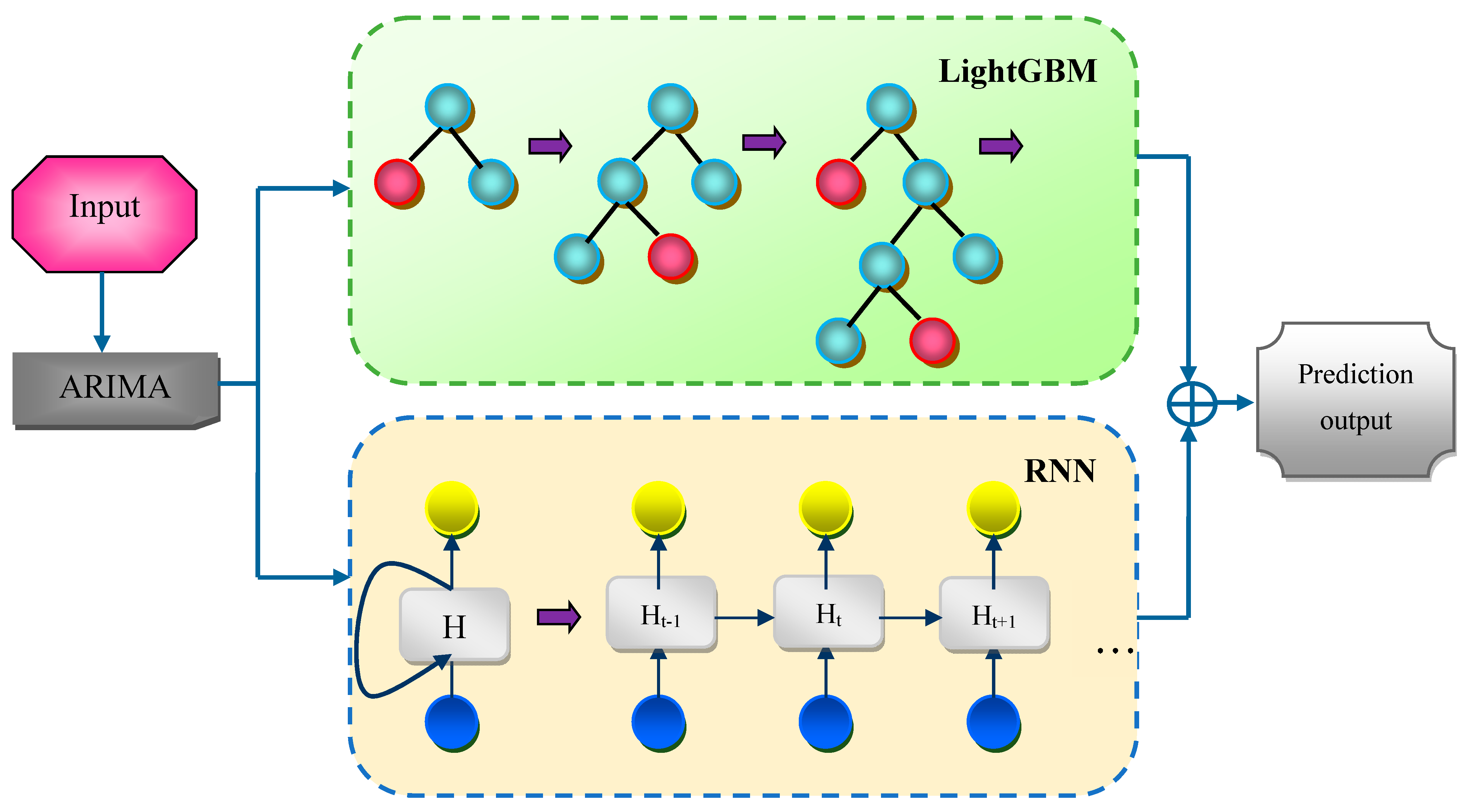
• Autoregressive integrated moving average ensemble recurrent light gradient boosting machine (AR-ERLM): The ensemble AR-ERLM model combines the strengths of decision trees and gradient boosting, resulting in accurate predictions. Furthermore, the RNN can learn long-term dependencies, allowing them to capture patterns over extended periods and automatically extract relevant features, which reduces the need for manual feature extraction.

The article’s remaining sections are structured as follows: Section 2 explores the review of the literature, and Section 3 describes the proposed methodology for stock movement prediction. The research findings, performance, and comparative evaluations of the AR-ERLM model are demonstrated in Section 4. Section 5 concludes the research with future works.

2. Literature Review

The literature papers related to Stock Movement Prediction are categorized, and the merits and demerits are described as follows:

(i)

Statistical models

Jiang et al. [14] utilized the ARIMA model for estimating future stock price values. Since ARIMA is highly adept at handling time series data, the model has shown superior prediction outcomes, making it a good choice for predicting the future stock index. The significance of stock price forecasting lies in the model’s prediction to mitigate losses mostly caused by faulty intuitions and blind investment.

Constandina Koki et al. [15] suggested the Bayesian Hidden Markov Model for predicting the cryptocurrency price. The NHHM model relies conditionally on the hidden states and determines the predictors with diverse linear and non-linear effects on the cryptocurrency returns. Further, the model demonstrates that the dominance of the predictive densities depends on the states that were captured in alternating periods with distinct return characteristics. However, frequent changes between the hidden states were found in all three time series, as the transitional patterns were markedly different.

(ii)

Machine Learning models

The ML method was used by Kittipob Saetia et al. [6], who analyzed the stock movement prediction from the technical indicators dataset. The ML model was highly capable of making out stocks with high future price growth in every aspect. However, the Pearson correlation coefficient was the only technique used to evaluate the relation between the stock movements and the keywords. Wasiat Khan et al. [7] employed an ML algorithm to improve the performance and quality of predictions, feature selection, and spam tweet reduction. The model has only the limited systematic techniques that were used for influential stocks relevant keywords while searching data on social media and news as well as for stock market forecast. Jordan Ayala et al. [9] provided an ML technique combined with Technical Analysis Indicators for stock movement prediction. The Technical indicator calculates the evaluation of the stock price. In this model, the decision-making workflow of trading has been used to evaluate the purchase and selling ratio of the stock value data. The executed model used a lesser amount of metrics than many others available. Kyung Keun Yun et al. [13] presented a hybrid GA-XGBoost technique to predict stock movements. The method was executed along with a three-stage feature engineering process, which achieved better results with more flexibility as the prediction time can be altered randomly. Technical indicator’s predefined numbers are only used in this method. However, the prediction model’s hyperparameters and model optimization should be improved for better performance and results.

Wei Chen et al. [11] implemented a portfolio construction technique using the ML-based prediction of Shanghai Stock Exchange asset data. The prediction model was developed using hybrid XGBoost, IFA, and mean-variance (MV) models to predict the stock movement more effectively than other traditional methods. The utilized dataset was highly affected by various economic backgrounds and political environments, which impacted the performance of the predictive model.

(iii)

Deep Learning models

Farnoush Ronaghi et al. [14] have established a hybrid deep-learning technique for stock movement forecasting. The established methods were used to compare the different classification metrics that calculate account productivity and cost levels of transactions to analyze the economic gains in stock market prediction. Additionally, this model can reduce the level of unneeded information and then potentially give better prediction results. The BiLSTM model has allowed for the learning of many more complex data structures, which also causes overfitting. Yaohu Lin et al. [5] utilized a hybrid deep learning technique to improve the prediction of the stock market movement. This presented technique performed exceptionally in both individual stock and multiple stock data based on their forecasting framework, and the given results have more précised values in every testing case. However, the executed method was not suited for predicting large-scale stock data. A DL method was modeled by Shuting Dong et al. [16] for stock movement prediction. For stock movement forecasting, the prediction model was dynamically evaluated and chosen via the dynamic predictor selection algorithm (DPSA). The time taken by the established method to train the networks and assess prediction performance was negligible. Additionally, compared to other traditional systems, this one achieved the best accuracy and highest return value since it made use of vast amounts of real-life financial time series data from the various stock markets. The daily upward and downward trend of the equities might not be predictable using the DPSA approach.

(iv)

Transformer Models

Chaojie Wang et al. [17] implemented the modern DL-based Transformer framework, which exploited the encoder–decoder architecture for predicting the stock market index. In this model, the transformer was initially utilized for the natural language processing problem and further adopted for time series forecasting. Compared with the typical CNN and RNN models, the Transformer model excels in its ability to extract crucial features, thereby obtaining efficient predictions. Still, there exist limitations as this approach only takes account of the single stock market index prediction, which is only one-dimensional time series data.

Zicheng Tao et al. [18] developed the Series decomposition Transformer, which uses the series decomposition layers and period-correlation mechanism to explore the relationship between historical series. In addition, the model effectively learned the alterations in the trends of the stock market, which resulted in high prediction performance and generalizability. However, the social information prevalent in multiple sources was difficult to collect, and a high level of uncertainty exists that affects the model’s prediction for different stock markets.

2.1. Challenges

• In the process of predicting financial variables, the existing large number of high correlation features contains a minimal amount of information, which increases the time complexity [14];
• The SVM approach proved to be computationally expensive for voluminous datasets and unsuitable for forecasting extensive stock data [5];
• The development of incorporating the market stock prices introduced obstacles such as misspellings, information duplication in text data, and shortcuts, causing low efficiency in output results [9];
• The DPSA model has limited ability to predict the daily downward and upward stock trends [15];
• The layered architecture in the ConvLSTM model increases the computational expenses and requires careful tuning [8];
• However, the proposed approach addressed the aforementioned challenges in the existing techniques via the application of the AR-ERLM model. Specifically, the AR-ERLM hybridizes the synergic strength of individual models, such as the potential of ARIMA for determining the linear dependencies, the ability of RNN to capture temporal dynamics, and LightGBM’s capability in handling the large-scale datasets and their non-linear relationships for achieving the effective stock price prediction. Consequently, the proposed approach improves the predictive accuracy, eliminates overfitting, and minimizes the computational overhead.

2.2. Problem Statement

Predicting stock market trends is a difficult but significant problem. The underlying nature of the stock market as a chaotic, noisy, dynamic, non-linear, and non-stationary system is the main reason for this. The financial system is inclined by a variety of interconnected and interplaying elements, such as general economic conditions, political developments, and trader expectations [2]. As a result, prediction of the stock movement trend index is very challenging and is still regarded as a significant time series research issue [8]. While the existing stock movement prediction tasks provide better results, they pose certain challenges, such as data overfitting, time complexity, and performance degradation problems [6]. Therefore, to mitigate these issues, this research proposes the AR-ERLM framework for effective stock movement prediction. Specifically, the proposed approach makes use of the ARIMA model to capture the linear dependencies in time series data, making the proposed approach effective for modeling stock prices that often show variations in trends and seasonality. Meanwhile, the RNN learns the long-term dependencies, facilitating the model to capture intricate patterns over a long time and eliminate the requirement for manual feature extraction. Ultimately, the ensemble AR-ERLM model integrates the potential of decision trees and gradient boosting in Light GBM for making accurate stock movement predictions [19].

3. Proposed AR-ERLM Model for Stock Movement Prediction

The key objective of the research is to effectively forecast stock movements using the AR-ERLM model. Initially, the Google trends data and the stock movements are collected from the live stream dataset [20,21,22]. Then, the Google trends and stock market data are combined using the daily and weekly binary calculations, which are then provided in the preprocessing stage, where data cleaning is performed. From the preprocessed data, the technical indicators are calculated, which is then subjected to the proposed AR-ERLM model, which leverages the benefits of ARIMA, which is a statistical model for time series analysis, RNN for capturing the temporal dynamics, and LightGBM for capturing the non-linear relationships in the complex time series data along with effectively handling the large-scale datasets. The proposed ensemble model effectively predicts stock market movement with better accuracy. The schematic illustration of the AR-ERLM model for stock movement prediction is illustrated in Figure 1.

3.1. Input for Stock Movement Prediction

In this research, the Google trends data and the stock market data of Amazon [20], Meta [21], and Netflix [22] are collected from Yahoo Finance, which is used to forecast stock movements. Further, these datasets comprise the history of daily prices of stocks such as Date field, open price, high price, low price, closing price, adjusted closing price, and trading volume attribute.

3.1.1. Stock Market Data

The data comprise high, low, volume, open, and close. Any listed stock’s opening price is its price at the beginning of the trading day. The lowest and highest price of stocks on that particular day is represented by the high and low values. The stock price at the end of the trading day is known as the closing price. Since the adjusted close price represents the stock’s value after shares are paid, it is recognized as the true price of that stock. Numerous factors affect stock prices, which are frequently used as indicators to examine market behavior. Therefore, analyzing technical indicators using the prices of securities increases the effectiveness of the understanding of market activity.

3.1.2. Google Trends Data

Google launched a service called Google Trends to assist in determining the popularity of terms such as brands, products, or websites. Users can view the popularity of these phrases in addition to the daily popular trends. Google Trends is intended for users who rely on or benefit from trends, whether they are marketers, operators of online stores, or even individuals who want to start a vlog but do not know what to sell or how to find the most searched terms every day or month. It also aids in the methodical formulation of marketing strategies and commercial plans.

3.2. Daily and Weekly Rolling Binary Calculation

In this research, the weekly trends represent the stock market trends that the general direction of the market price varying over time, and it is based on the demand for the four prominent tech stocks such as Amazon, Meta platform, Netflix, and Nifty50 are analyzed. Additionally, the daily prices of the stocks were obtained from Yahoo Finance. To improve prediction accuracy, the rolling binary calculation method is employed, which converts weekly trends into daily data and allows the capture of finer fluctuations. Furthermore, this research utilizes the real-time live dataset and is applicable for real-time prediction of stock movements. To determine the periods of important price declines from the historical time series data, the ratio of the current index level at time $t$ to the maximum index level over $q$ rolling periods prior to time $t$ is utilized, and transformed the index level series to the Maximum Level $MaxL$ sequence as follows:

$$Max{L}_t=G_t/\max \left(G_{t-q},G_{t-q+1},\dots G_t\right)$$

(1)

where $G_t$ denotes the closing price. In this stock movement prediction, one year is set as the rolling period for evaluating the above ratio. For instance, the ratio of 100% represents that the index level grows to the maximum value in the rolling period. Meanwhile, the low value of $MaxL$ denotes the decline in price over the rolling period. Further, the binary crisis variable is developed considering the sequence of cutoff values, which requires taking the difference between the moving averages of the ratio and the factor of moving standard deviations. Further, the binary crisis indicator is expressed as follows:

$$c{c}_t=\left\{\begin{array}{l}1 if Max{L}_t<\overline{Max{L}_t}-2.5{\sigma }_t\\ 0 otherwise\end{array}\right.$$

(2)

where ${\sigma }_t$ indicates the standard deviation over the rolling period, $\overline{Max{L}_t}$ represents the mean value of $MaxL$ ranging from $t-q$ to $t-1$. In Equation (2), the mean value and the standard deviation are calculated for the first 250 trading days. Further, the first day of the sample is subtracted, and an extra day is added at a time to evaluate the statistics in each of the following days.

3.3. Data Preprocessing

Preparing raw data for analysis, particularly for market movement prediction, requires data preprocessing. Here, data cleaning is performed to identify and remove irrelevant data, including dates that do not contribute to the analysis. Data preprocessing ensures data quality and reliability, leading to better decision-making.

3.4. Technical Indicators

Technical indicators are helpful in forecasting asset prices in the future, which is important for incorporating them into automated trading systems. Technical indicators are frequently employed by active traders designed to assess short-term price movements. However, long-term investors can also utilize technical indicators to identify entry and exit locations.

3.4.1. Moving Average

The MA uses the average closing price over a given period to produce moving averages, smooths and filters numerous aberrant signals to show the average trend over that period, which is defined as

$$I_{MA}={\displaystyle \frac{G_t+G_{t-1}+G_{t-2}+\dots G_{t-n+1}}{n}}$$

(3)

where $n$ indicates the time interval and the close price is signified as $G$.

3.4.2. Bollinger Bands (BB)

The BB is a volatility indicator that tracks an upper and lower band utilizing two standard deviations.

3.4.3. Relative Strength Index (RSI)

RSI helps gauge market momentum by assigning a value between 0 and 100 that indicates whether an asset is overbought or oversold.

$$I_{RSI}\left(t\right)=100\ast {\displaystyle \frac{U_{Avg}\left(t\right)}{U_{Avg}+D_{Avg}}}$$

(4)

where $U_{Avg}$, $D_{Avg}$ indicates the upward and the downward average price movement, respectively.

3.4.4. Money Flow Index (MFI)

The MFI measures the flow of money in and out of security, which is mathematically calculated as follows:

$$I_{MFI}\left(t\right)=100-{\displaystyle \frac{100}{1+MR\left(t\right)}}$$

(5)

where $MR\left(t\right)$ denotes the money ratio.

3.4.5. Average True Range (ATR)

ATR breaks down the whole range of a stock’s or asset’s price over a given period to determine the volatility of finance markets.

$$I_{ATR}\left(t\right)={\displaystyle \frac{1}{n}}{\displaystyle \sum _{j=1}^{n}TR\left(t-j+1\right)}$$

(6)

where $TR$ indicates the true range.

3.4.6. Force Index

The volume, magnitude, and direction of the stock price change are all considered by the force index. These three components combine to create an oscillator that gauges the pressure to purchase and sell.

3.4.7. Ease of Movement Value (EMV)

An oscillator called EMV aims to combine volume and price into a single quantity. Assessing the strength of a trend is helpful because it considers both price and volume.

3.4.8. Aroon Indicator

Aroon indicator [23] is used to spot shifts in an asset’s price trend and gauge the strength of the trends. The indicator counts the intervals between highs and lows for a given period.

3.4.9. Aroon up Channel

The strength of the uptrend is measured by the Aroon up channel, which is represented as follows:

$$I_{Aup}=\left[{\displaystyle \frac{CP-N{P}_{days}}{CP}}\right]\ast 100$$

(7)

where $CP$ indicates the calculation period, and $N{P}_{days}$ represents the number of days following the highest price.

3.4.10. Aroon Down Channel

The strength of the downtrend is measured by the Aroon down channel, which is represented as follows:

$$I_{Aup}=\left[{\displaystyle \frac{CP-N{L}_{days}}{CP}}\right]\ast 100$$

(8)

where $N{L}_{days}$ denotes the number of days following the lowest price.

3.4.11. MA Convergence Divergence (MACD)

MACD is defined as the difference between the two exponential moving averages [24], which can be evaluated as follows:

$$I_{MACD}\left(t\right)={\displaystyle \sum _{i=1}^n{I}_{EM{A}_{12d}}}-{\displaystyle \sum _{i=1}^n{I}_{EM{A}_{26d}}}$$

(9)

where $I_{EMA}$ denotes the exponential moving average.

3.4.12. MACD Histogram

The MACD’s background includes a histogram, which shows the difference between the signal line $\left(SL\right)$ and the MACD that is mathematically defined as

$$H_{MACD}=lin{e}_{MACD}-SL$$

(10)

where $lin{e}_{MACD}$ denotes the MACD line.

3.4.13. MACD Signal Line

The signal line serves as the basis for interpretation. When the MACD is above the signal line, the bar is positive; when the MACD is below the signal, it is negative.

3.4.14. Exponential Moving Average (EMA)

The EMA is a technical indicator that is employed to track the price of a stock.

$$I_{EMA}\left(t\right)={\displaystyle \frac{2}{n+1}}{G}_t{\displaystyle \frac{n-1}{n+1}}{I}_{EMA\left(t-1\right)}$$

(11)

where $G_t$ represents the index value at the time $t$.

3.4.15. Simple Moving Average (SMA-50)

SMA is computed by dividing the average of a given range of prices and the total number of periods within that range.

$$I_{SMA}\left(t\right)={\displaystyle \frac{1}{n}}\left(Z\ast I_{MA}\left(t\right)\right)+\left(n-Z\right)\ast I_{SMA}\left(t-1\right)$$

(12)

where $Z$ indicates the weights.

3.4.16. SMA-200

The SMA 200 is computed using the average price of the last 200 days with the daily price chart as well as other MA.

3.4.17. Weighted Moving Average (WMA)

The WMA assigns more weight to the present data, which is used to determine the trade trends.

3.4.18. Triple Exponential Average (TRIX)

The TRIX is also used as a momentum indicator, which determines the percentage change of moving averages as well as the difference between the smoothed version of price information.

3.4.19. Mass Index

The mass index is used to forecast the trend reversal, which is measured between the range of high and low stock prices.

3.4.20. Ichimoku Kinko Hyo Span A

Ichimoku means one look in Japanese, which implies that traders simply need to glance at the chart to identify momentum, support, and resistance. Senkou Span A, often known as Leading Span A, is one of the Ichimoku Cloud indicator’s five components. The Leading Span A line is a momentum indicator that can suggest trades depending on levels of support and resistance.

3.4.21. Ichimoku Kinko Hyo Span B

A Kumo is a cloud formation that is created when the Leading Span B and the Senkou Span A line combine. Levels of resistance and assistance are offered by the cloud.

3.4.22. Know Sure Thing (KST)

To predict the momentum of price movements in several markets, they are identified using the KST indicator.

3.4.23. Detrended Price Oscillator (DPO)

To measure the distance between the peaks and troughs in the price/indicator. DPO helps traders predict future peaks in selling and buying opportunities.

3.4.24. Commodity Channel Index (CCI)

CCI is used to evaluate the variation between the current and the historical average price, which can be mathematically computed as

$$I_{CCI}={\displaystyle \frac{\frac{h_t+lo{w}_t+G_t}{3}-I_{MA}\left(n\right)}{0.015\ast \frac{1}{n}{\displaystyle {\sum }_{i-n}^n{I}_{MA}\left(i\right)-G_i}}}$$

(13)

where $h_t,lo{w}_t$ indicates the high and low prices, respectively.

3.4.25. Average Directional Index (ADX)

The ADX is an oscillator that measures the strength of trends. The mathematical equation for ADX is defined as follows:

$$I_{ADX}\left(t\right)={\displaystyle \frac{I_{ADX}\left(t-1\right)\ast \left(n-1\right)+I_{DX}\left(t\right)}{n}}$$

(14)

where $n$ denotes the period and $I_{DX}\left(t\right)$ indicates the directional movement index.

3.4.26. Minus Directional Indicator (–DI)

The presence of a downtrend is measured using –DI, which is described using the following equation:

$$-I_{DI}={\displaystyle \frac{Sm-DM}{TR}}$$

(15)

where $-DM$ represents the negative directional movement, $Sm$ indicates the smoothened value.

3.4.27. Plus Directional Indicator (+DI)

The presence of an uptrend is measured using +DI, which is described using the following equation

$$+I_{DI}=\left({\displaystyle \frac{Sm+DM}{TR}}\right)100$$

(16)

3.4.28. Schaff Trend Cycle (STC)

STC is used to calculate the velocity of price movements. Further, the obtained technical indicators assist in identifying the potential reversal points and trend direction as well as provide more statistical parameters for evaluation. In this research, the technical indicators are fed into the proposed AR-ERLM model to make predictions about the stock movement.

3.5. Autoregressive Integrated Moving Average Ensemble Recurrent Light Gradient Boosting Machine for Stock Movement Prediction

Stock movement forecasting is a major task in the economic world, but because of the non-linear characteristics of data, it remains challenging. Several ML and DL approaches have been developed in recent years; while the established techniques attained better results, they also posed certain inherent limitations. The XGBoost was an effective ML technique mostly used by various authors [9,11,13], which provides accurate predictions due to its ensemble of decision trees and regularization techniques. It also handles noise and outliers well, making it suitable for stock movement prediction tasks. However, XGBoost does not directly handle categorical features and can be memory-intensive for large datasets. Furthermore, the convolutional neural network with long short-term memory (CNN-LSTM) was utilized by previous studies [8,14] to significantly obtain pertinent features from raw data, while LSTM captures temporal dependencies that also modeled complex, non-linear relationships in stock data. Nevertheless, combining CNN and LSTM introduced additional complexity, which required careful tuning. Training could be computationally expensive due to the layered architecture. The random forest [3] classifier designed for stock movement prediction handles noise and outliers well, making it subtle for stock prediction, which also requires minimal parameters for training as well as effectively handling large datasets. Despite their advantages, the linear assumptions did not capture the dynamic nature of stock market data. Artificial Neural Networks (ANN) [25] could capture complex patterns and non-linear relationships as well as handle different data styles and structures. However, if not properly regularized, the ANN technique was prone to overfitting.

To overcome the above-mentioned limitations of the existing techniques, this research presented an AR-ERLM model that is designed using the ensemble LightGBM and RNN classifiers and utilizes the ARIMA features for effective stock movement prediction. ARIMA captures trends and seasonality in time series data. Further, the RNN-LightGBM handles non-linear relationships and feature extraction. The architecture of the AR-ERLM model for stock movement prediction is shown in Figure 2.

Initially, the technical descriptors obtained from the input data are provided in the ARIMA model, which is a significant technique used in prediction tasks of time series analysis, also known as the Box–Jenkins method. ARIMA is a technique that synthesizes historical data patterns to produce forecasts. When it comes to forecasting, parameter estimation, and univariate time series model identification, the ARIMA approach gives a great deal of versatility [26]. The generated time series is derived as follows [27]:

$$g_t={\theta }_0+{\varphi }_1{g}_{t-1}+{\varphi }_2{g}_{t-2}+\dots \dots {\varphi }_Q{g}_{t-Q}+{\xi }_t-{\theta }_1{\xi }_{t-1}-{\theta }_2{\xi }_{t-2}-\dots \dots {\theta }_P{\xi }_{t-P}$$

(17)

where $g_t$ signifies the stationary value series, ${\xi }_t$ indicates the random error at $t$, the model parameters are signified as ${\varphi }_i\left(i=1,2,\dots Q\right)$ and ${\theta }_l\left(l=1,2,\dots P\right)$. The integers $Q$ and $P$ are frequently referred to as the model’s order. It is assumed that random errors ${\xi }_t$ have a mean of zero and a constant variance of ${\sigma }^2$. They are also assumed to be identically and independently distributed. For an ARIMA model to be effective in forecasting, stationary is a prerequisite. The feature of a stationary time series is that it maintains consistent statistical properties throughout time, such as the mean and the autocorrelation structure. When the observed time series shows heteroscedasticity and trend, differencing and power transformation are often used to the data to remove trends and stabilize variance before an ARIMA model can be fitted. Estimating the model parameters is simple, and to minimize the overall measure of errors, the parameters are calculated using the non-linear optimization technique. The output obtained from the ARIMA model $\left(g_t\right)$ is provided as input for both LightGBM and RNN models simultaneously.

LightGBM uses a tree-based learning algorithm created by Microsoft. LightGBM uses gradient-based one-side sampling (GOSS) and exclusive feature bundling (EFB) to shorten training times without sacrificing accuracy. Additionally, it builds trees using a leaf-wise growth strategy and histogram-based techniques for data binning, leading to faster convergence and improved performance [28]. A technique for effective gradient boosting with big datasets is called GOSS, which involves sampling the data points according to their gradients, and the probability of small data points being selected in training is lower. Consequently, GOSS lowers the quantity of data points needed for training without compromising the model’s overall performance. In contrast, EFB is a feature bundling technique that reduces the number of features utilized for training by combining related characteristics. EFB can assist in lowering the computational cost of training and increase model accuracy by grouping features [29]. GOSS and EFB, when coupled with other methods such as leaf-wise tree growth and histogram-based binning, have enabled AR-ERLM to attain better performance in stock movement prediction tasks, particularly for high-dimensional and large-scale datasets. By using the $R$ additive functions of the LightGBM, the AR-ERLM model can predict the outcome, which is detailed as follows [30]:

$${\widehat{z}}_t={\displaystyle \sum _{j=1}^R{f}_j\left(g_t\right)},f_j\in F$$

(18)

Here, $f_j$ denotes the function in the functional space $F$, which can be expressed as

$$f_j\left(g_t\right)=u_{d\left(g_t\right)}, u\in {ℝ}^N, d:{ℝ}^m\to \left\{1,2,\dots N\right\}$$

(19)

where $N$ denotes the number of leaves, $u$ represents vector sores on leaves, and $d$ is a function that links each data point to its corresponding leaf. The set of all potential functions based on various pairings of $d$ and $u$ is captured by $F$. The objective function $\left(O\right)$ that needs to be optimized is derived as follows:

$$O={\displaystyle \sum _{k=1}^{n}L\left(z_t,{\widehat{z}}_t\right)+{\displaystyle \sum _{j=1}^R\varpi \left(f_j\right)}}$$

(20)

where the regularization term $\varpi \left(f_j\right)$ is used to penalize the model’s complexity and $L$ is a loss function that quantifies the variation between the raw prediction ${\widehat{z}}_t$ and the target $z_t$. The regularization term can be defined as

$$\varpi \left(f_j\right)=\lambda N+{\displaystyle \frac{1}{2}}\gamma {\displaystyle \sum _{j=1}^R{u}_j^2}$$

(21)

where $\gamma$ and $\lambda$ indicates the learning parameters. AR-ERLM uses histogram-based techniques to bin data into discrete intervals, which lowers computing costs and memory utilization.

RNN is a variant of neural networks where the units are connected recurrently, enabling them to process the incoming sequence using their internal memory. This makes it possible to employ AR-ERLM for the stock market prediction tasks. In this research, AR-ERLM is employed because stock data requires consideration of long-term dependencies [31] in the data. The computing units of the model have a configurable weight and real-valued activation that varies over time. The same set of weights is applied recursively over a structure resembling a graph to construct AR-ERLM. The input $g_t$ at the current time step and the preceding hidden state $H_{t-1}$ are used to evaluate the hidden state.

$$H_t=\tanh \left(p{g}_t+q{H}_{t-1}+b\right)$$

(22)

$$Y_t=\tanh \left(w{H}_t+c\right)$$

(23)

where $Y_t$ denotes the output, RNN-trained input-to-hidden, hidden-to-hidden, and hidden-to-output parameters are $p$, $q$, and $w$, respectively. Because the learned model in an AR-ERLM is defined in terms of the transition from one state to another, it always has the same input size. Additionally, for each time step, the design employs the same transition function with the same parameters. To provide the final prediction output $\left(D_t\right)$, the AR-ERLM model combines the output of both models using the following equation:

$$D_t=Y_t\oplus {\widehat{z}}_t$$

(24)

where the symbol $\oplus$ indicates the concatenation operation.

The AR-ERLM model predicts the stock movement effectively. The proposed model excels in capturing linear relationships and trends in time series data, while the RNN is adaptable at learning from sequential data with their internal memory, making them suitable for recognizing patterns over time. In addition, the gradient boosting technique effectively handles large datasets and improves performance through its tree-based learning techniques. Therefore, the AR-ERLM model predicts stock with better accuracy.

4. Results and Discussion

The experimental results evaluated using the AR-ERLM model for stock movement prediction, as well as the comparative and performance analysis, are described in the following section.

4.1. Experimental Setup

The research for stock movement prediction using the AR-ERLM model is conducted in Python software V 3.10 on a Windows 10 operating system with 16 GB of RAM. The initial parameter settings of the proposed network involve a batch size of 32, a learning rate of 0.001, a dropout rate of 0.02, a linear activation function, and a loss function “MSE”, optimized utilizing the default optimizer, Adam.

4.2. Performance Metrics

The performance of the AR-ERLM model in the stock movement prediction task is analyzed using the following performance metrics: Mean Absolute Error (MAE), RMSE, Mean Absolute Percentage Error (MAPE), and MSE. Outliers and imbalances in the dataset can be found using MSE, which calculates the average of the squared discrepancies between the actual and predicted values. The standard deviation of the error is measured by RMSE, which is the square root of MSE and makes model comparisons simple. RMSE makes it simple to compare model performances. The most accurate model is the one with the lowest RMSE value. The error is expressed as a percentage of the actual value using MAPE.

4.3. Dataset Description

In this research, the weekly trends of three prominent technical stocks such as Amazon [20], Meta platform [21], Netflix [22], and Nifty50 [32] are analyzed. Additionally, the daily prices of the stocks were obtained from Yahoo Finance. Further, these datasets comprise the history of daily prices of stocks such as Date field, open price, high price, low price, closing price, adjusted closing price, and trading volume attribute to carry out the implementation of the stock movement prediction. Further, the four stocks, including the Amazon, Meta platform, Netflix, and Nifty50, are utilized for the prediction as the Netflix stock operates as the world’s most-subscribed streaming service. In addition, the Meta data and Amazon stocks are progressing and providing impressive returns, significantly outperforming the e-commerce market. Meanwhile, the NIFTY 50 is an Indian stock market index indicating the float-weighted average of 50 of the Major Indian companies listed on the National Stock Exchange. Moreover, the proposed approach analyzed the stock data collected from the current to the last 5 years to attain efficient stock movement prediction.

4.4. Comparative Methods

In this research, the performance of the AR-ERLM model is compared with the other presented techniques such as XGBoost [6], Artificial Neural Network (ANN) [25], Improved Firefly Algorithm enabled XGBoost (IFA-XGBoost) [11], Genetic Algorithm LightGBM (GA-LightGBM) [33], ARI-MA-LS-SVM [34], ANN-SVM [35], Convolutional LSTM (ConvLSTM) [16].

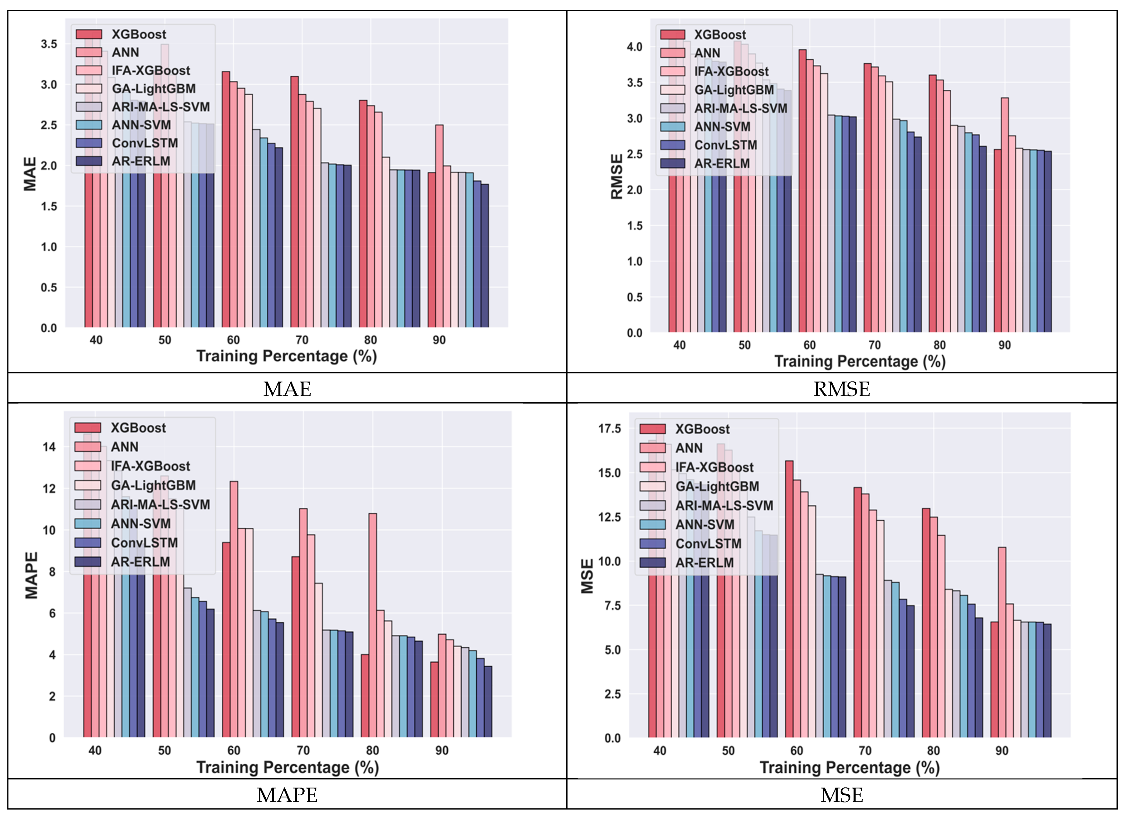
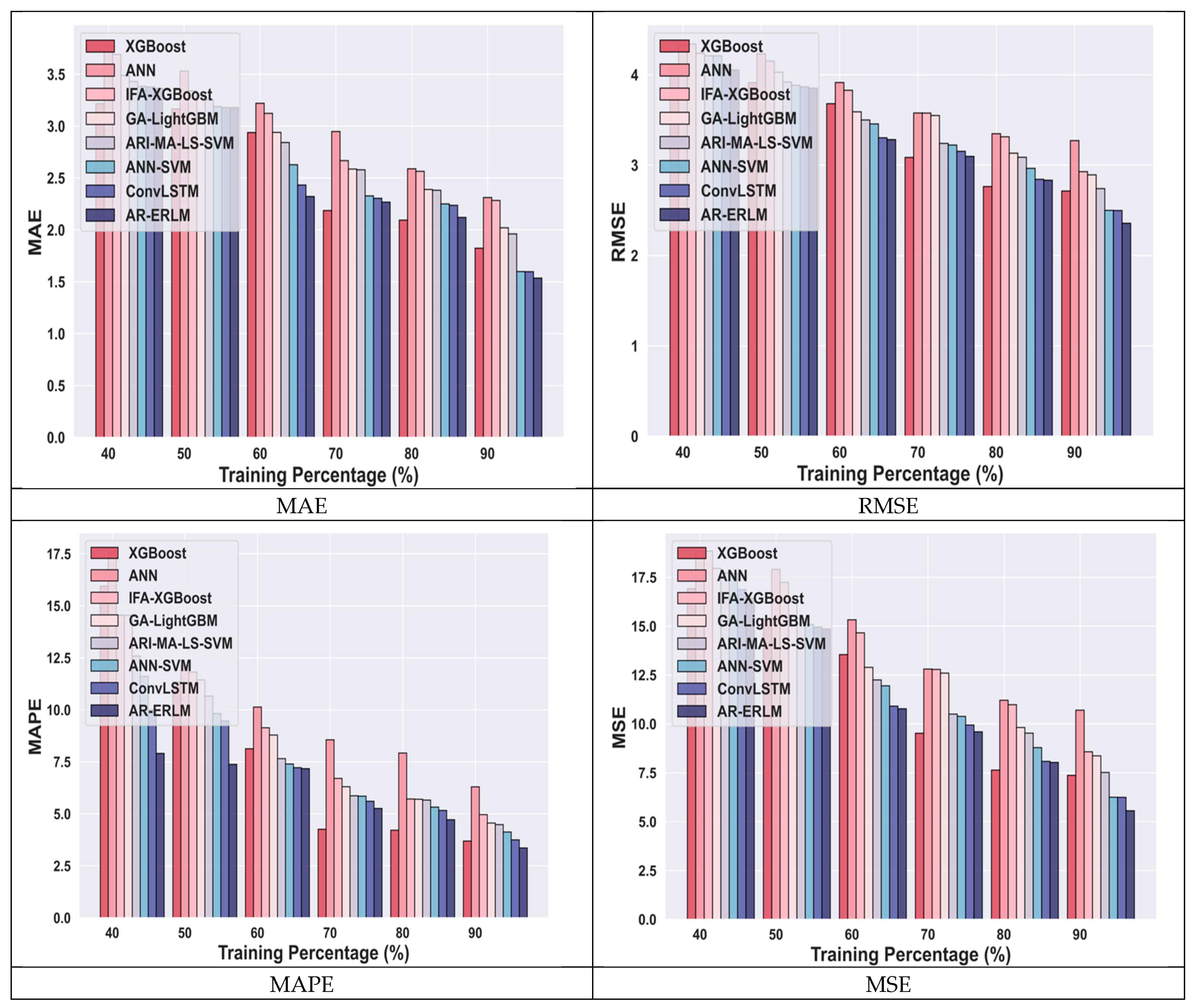
4.4.1. Comparative Analysis for Meta Data Using Training Percentage

The comparative evaluation of the AR-ERLM model to predict stock movements using the Meta data in terms of RMSE, MAPE, MAE, and MSE is depicted in Figure 3. For the Training Percentage (TP) 90, the AR-ERLM model attained an MAE of 1.77, which is comparably less than XGBoost by 0.14, ANN by 0.73, IFA-XGBoost by 0.23, GA-LightGBM by 0.15, ARI-MA-LS-SVM by 0.15, ANN-SVM by 0.14, and ConvLSTM by 0.04. Similarly, for the RMSE measure, the AR-ERLM model gets 2.53, which is reduced over the traditional XGBoost by 0.02, ANN by 0.75, IFA-XGBoost by 0.22, GA-LightGBM by 0.04, ARI-MA-LS-SVM by 0.022, ANN-SVM by 0.018, and ConvLSTM by 0.01. In terms of MSE, the AR-ERLM model conquers a minimal value of 6.43, reduced by 0.13 over XGBoost, 4.34 over ANN,1.139 over IFA-XGBoost,0.21 over GA-LightGBM, 0.12 over ARI-MA-LS-SVM, 0.11 over ANN-SVM, and 6.53 over ConvLSTM. Subsequently, the AR-ERLM model attains the low error of 3.43, which is minimized by 0.20 over XGBoost, 1.54 over ANN, 1.28 over IFA-XGBoost, 0.97 over GA-LightGBM, 0.90 over ARI-MA-LS-SVM, 0.75 over ANN-SVM, and 0.38 over ConvLSTM. From the comparative results, it is clear that the AR-ERLM model efficiently predicts stock movements with minimal errors. Furthermore, the proposed model excels in capturing linear relationships and trends in time series data, while the RNN adapts to learning from sequential data with their internal memory, making them suitable for recognizing patterns over time as well, and the gradient boosting technique effectively handles large datasets and improves performance through its tree-based learning techniques.

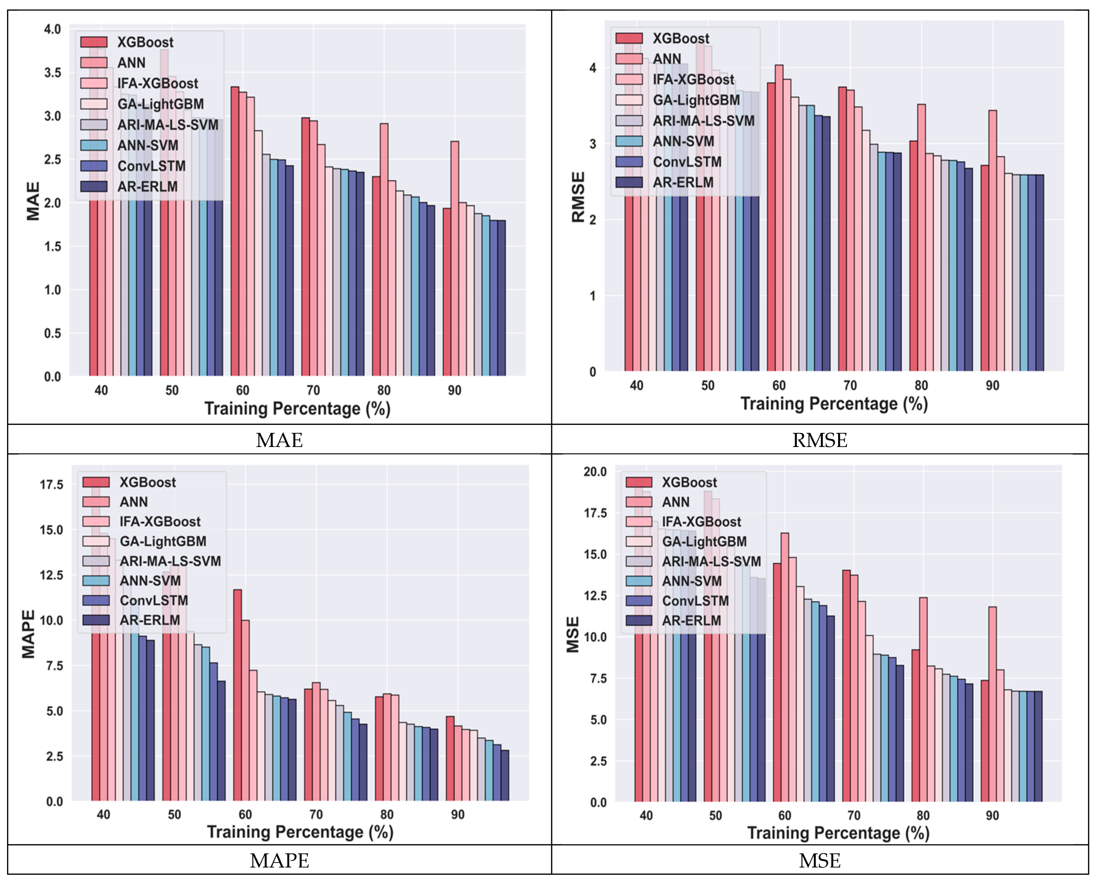
4.4.2. Comparative Analysis for Amazon Data Using TP

The comparative analysis of the AR-ERLM model for predicting stock movements using Amazon data, based on metrics such as RMSE, MAE, MAPE, and MSE, is delineated in Figure 4. For TP 90, the AR-ERLM model achieved an MAE of 1.65, which is notably lower than XGBoost by 0.13, ANN by 0.91, IFA-XGBoost by 0.20, GA-LightGBM by 0.17, ARI-MA-LS-SVM by 0.07, ANN-SVM by 0.05, and ConvLSTM by 0.01. Similarly, the RMSE measure for the AR-ERLM model is 2.588, reduced over the traditional XGBoost by 0.12, ANN by 0.84, IFA-XGBoost by 0.24, GA-LightGBM by 0.01, ARI-MA-LS-SVM by 0.02, ANN-SVM by 0.03, ConvLSTM by 0.01. In terms of MSE, the AR-ERLM model outperforms other established techniques with a minimal value of 6.702, obtaining an error difference of 0.66 against XGBoost, 5.10 against ANN, 1.30 against IFA-XGBoost, 0.09 against GA-LightGBM, 0.01 against ARI-MA-LS-SVM. In terms of MAPE, the AR-ERLM model conquers a minimal value of 2.81 achieving the error difference of 1.86, 1.34, 1.14, 1.09, 0.67, 0.54, and 0.31 over the other established techniques such as XGBoost, ANN, IFA-XGBoost, GA-LightGBM, ARI-MA-LS-SVM, ANN-SVM, and ConvLSTM, respectively. These comparative results highlight the efficacy of the AR-ERLM model in predicting stock movements with minimal errors. Additionally, the model excels in capturing linear relationships and trends in time series data, while RNNs are adept at learning from sequential data due to their internal memory, making them suitable for recognizing patterns over time. Meanwhile, the gradient boosting technique effectively handles large datasets and enhances performance through its tree-based learning approach.

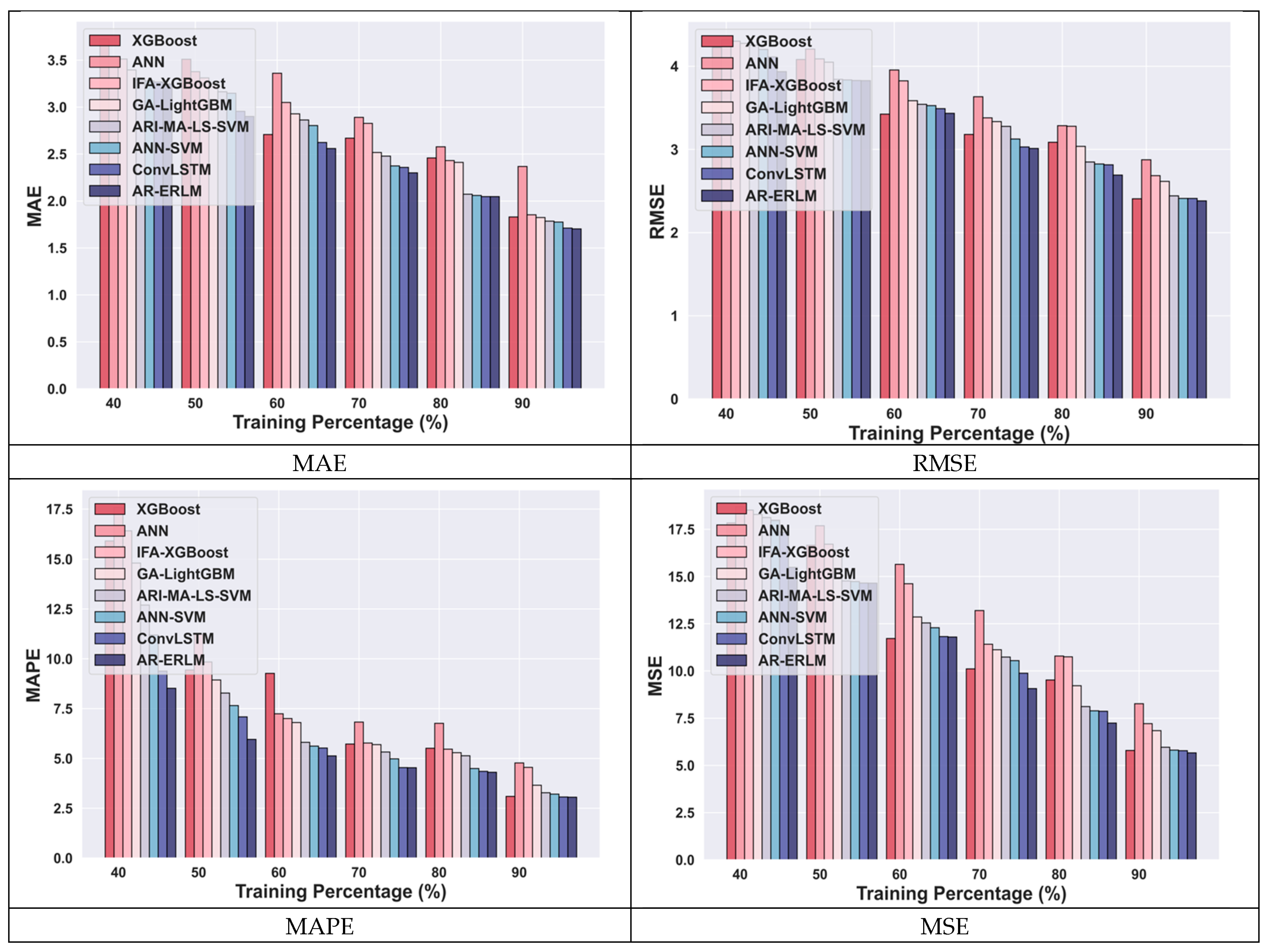
4.4.3. Comparative Analysis for Netflix Data

The comparative analysis of the AR-ERLM model for predicting stock movements using Netflix data regarding metrics such as MAPE, MAE, RMSE, and MSE is delineated in Figure 5. For TP 90, the AR-ERLM model achieved an MAE of 1.70, which is notably lower than XGBoost by 0.12, ANN by 0.66, IFA-XGBoost by 0.15, GA-LightGBM by 0.12, ARI-MA-LS-SVM by 0.08, ANN-SVM by 0.07. Similarly, the RMSE measure for the AR-ERLM model is 2.38, showing an error difference of 0.2 over XGBoost, 0.49 over ANN, 0.30 over IFA-XGBoost, 0.23 over GA-LightGBM, 0.06 over ARI-MA-LS-SVM, 0.03 over ANN-SVM, and 0.03 over ConvLSTM. In terms of MSE, the AR-ERLM model outperforms other established techniques with a minimal value of 5.66, reduced over the existing technique XGBoost by 0.123, ANN by 2.60, IFA-XGBoost by 1.54, GA-LightGBM by 1.17, ARI-MA-LS-SVM by 0.29, ANN-SVM by 0.14, and ConvLSTM by 0.11. In terms of MAPE, the AR-ERLM model conquers a minimal value of 3.05, achieving an error difference of 0.04 over XGBoost, 1.72 over ANN, 1.49 over IFA-XGBoost,0.59 over GA-LightGBM, 0.22 over ARI-MA-LS-SVM,0.15 over ANN-SVM, and 0.019 over ConvLSTM. These comparative results highlight the efficacy of the AR-ERLM model for stock movement prediction with minimal errors. Additionally, the model excels in capturing linear relationships and trends in time series data, while RNNs are adept at learning from sequential data due to their internal memory, making them suitable for recognizing patterns over time. Meanwhile, the gradient boosting technique effectively handles large datasets and enhances performance through its tree-based learning approach.

4.4.4. Comparative Analysis for Nifty50 Using Training Percentage

The comparative evaluation of the AR-ERLM model with other existing methods for predicting stock movements using Nifty50 data, in terms of metrics MAPE, MAE, RMSE, and MSE, is illustrated in Figure 6. For 90% of training, the AR-ERLM model attained the MAE score of 1.81, which is significantly lower than XGBoost by 0.45, ANN by 0.72, IFA-XGBoost by 0.48, GA-LightGBM by 0.36, ARI-MA-LS-SVM by 0.24, ANN-SVM by 0.08, and ConvLSTM by 0.05. Similarly, the RMSE for the AR-ERLM model is 2.39, outperforming the other existing techniques with the error difference of 0.66 over XGBoost,0.67 over ANN, 0.59 over IFA-XGBoost,0.50 over GA-LightGBM, 0.49 over ARI-MA-LS-SVM,0.30 over ANN-SVM, and 0.13 over ConvLSTM. In terms of MSE, the AR-ERLM model surpasses other existing techniques with a minimal value of 5.71, minimized over the other existing technique XGBoost by 3.58, ANN by 3.64, IFA-XGBoost by 3.14, GA-LightGBM by 2.65, ARI-MA-LS-SVM by 2.57, ANN-SVM by 1.51, and ConvLSTM by 0.65. In terms of MAPE, the AR-ERLM model attains a minimal value of 2.54, achieving an error difference of 1.86 over XGBoost, 4.93 over ANN, 3.76 over IFA-XGBoost, 2.20 over GA-LightGBM, 1.80 over ARI-MA-LS-SVM, 1.76 over ANN-SVM, and 0.87 over ConvLSTM. From the comparative evaluation, the AR-ERLM model attained minimal errors for stock movement prediction due to its high potential in capturing the non-linear relationships and trends in complex time series data. Moreover, the proposed approach attained low error values for the stock movement prediction and outperformed other baseline techniques utilized for comparison.

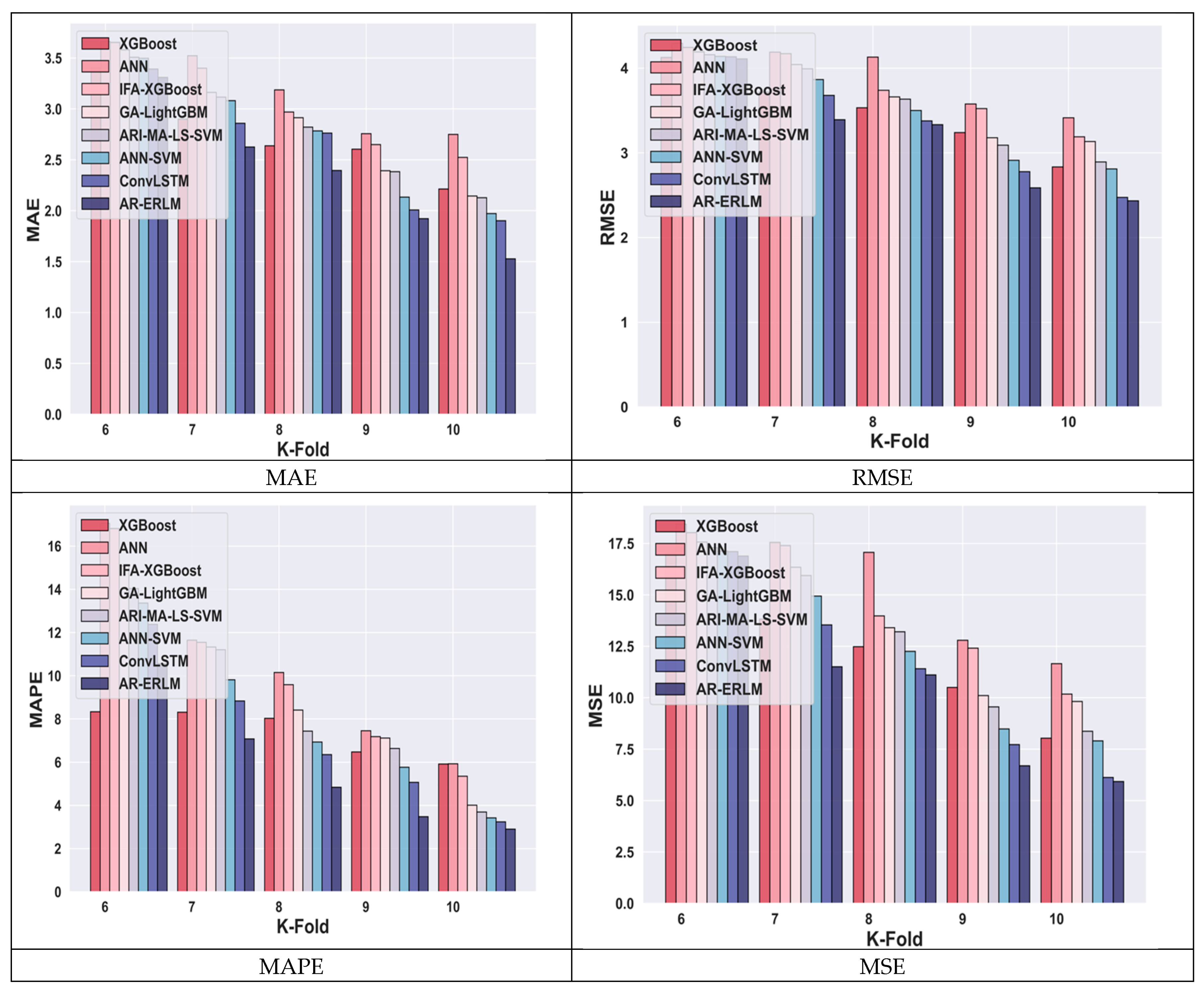
4.4.5. Comparative Analysis for Meta Data Using k-Fold

The comparative evaluation of the AR-ERLM model to predict stock movements using the Meta data in terms of RMSE, MAPE, MAE, and MSE is depicted in Figure 7. For the k-fold 10, the AR-ERLM model attained an MAE of 1.58, which is comparably less than XGBoost by 0.20, ANN by 0.58, IFA-XGBoost by 0.45, GA-LightGBM by 0.26, ARI-MA-LS-SVM by 0.15, ANN-SVM by 0.08, and ConvLSTM by 0.02. Similarly, for the RMSE measure, the AR-ERLM model gets 2.47, which is reduced over the traditional XGBoost by 0.06, ANN by 0.53, IFA-XGBoost by 0.33, GA-LightGBM by 0.29, ARI-MA-LS-SVM by 0.03, ANN-SVM by 0.029, and ConvLSTM by 0.02. In terms of MSE, the AR-ERLM model conquers a minimal value of 6.10, reduced by 0.30 over XGBoost, 2.95 over ANN,1.76 over IFA-XGBoost, 1.56 over GA-LightGBM,0.16 over ARI-MA-LS-SVM,0.14 over ANN-SVM, and 0.10 over ConvLSTM. Subsequently, the AR-ERLM model attains the low error of 3.12, which is minimized by 0.61 over XGBoost, 2.35 over ANN,1.29 over IFA-XGBoost, 1.02 over GA-LightGBM, 0.80 over ARI-MA-LS-SVM, 0.37 over ANN-SVM, and 0.06 over ConvLSTM. From the comparative results, it is clear that the AR-ERLM model efficiently predicts stock movements with minimal errors. Furthermore, the proposed model excels in capturing linear relationships and trends in time series data, while the RNN adapts to learning from sequential data with their internal memory, making them suitable for recognizing patterns over time as well, and the gradient boosting technique effectively handles large datasets and improves performance through its tree-based learning techniques.

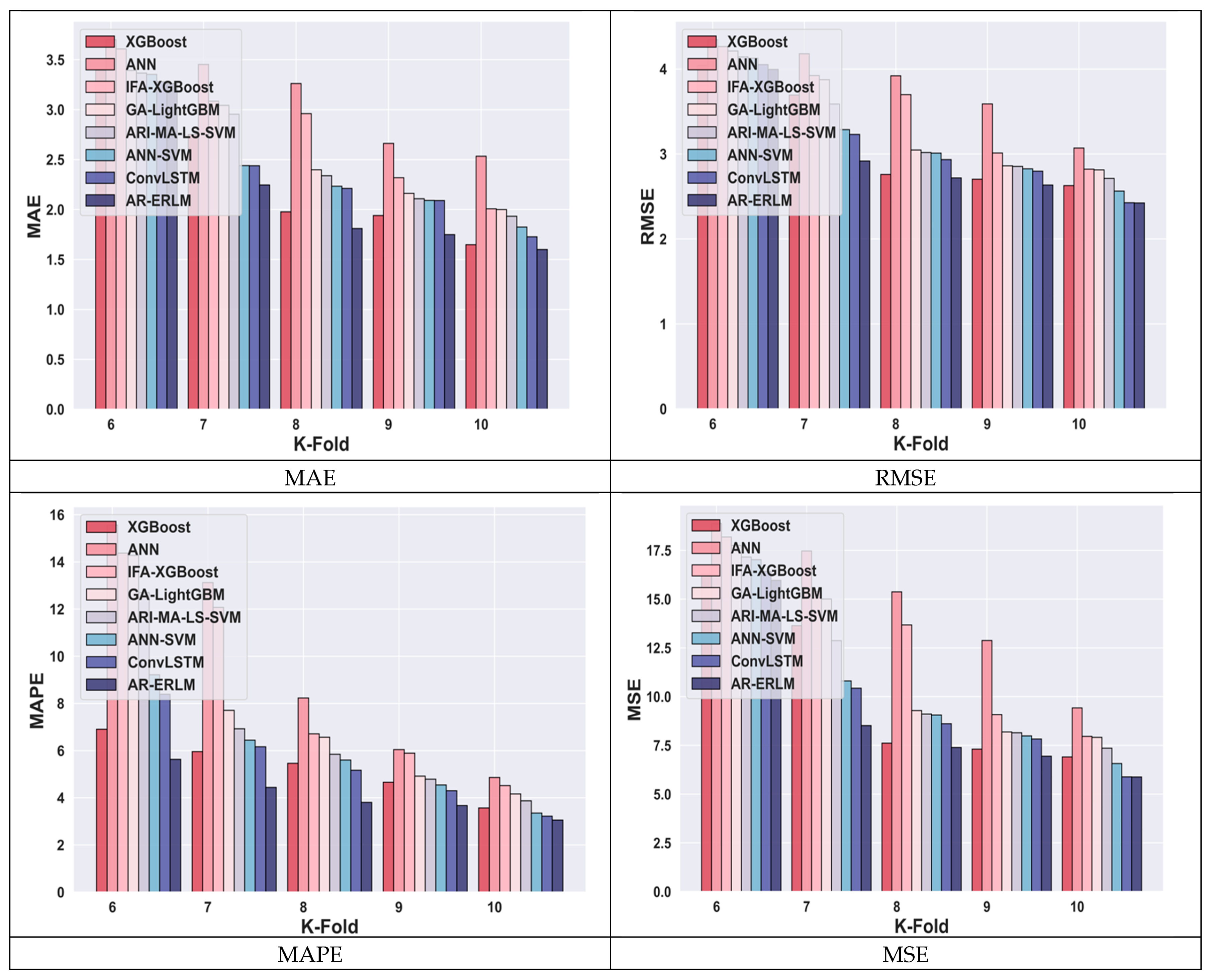
4.4.6. Comparative Analysis for Amazon Data Using k-Fold

The comparative analysis of the AR-ERLM model for predicting stock movements using Amazon data, based on metrics such as RMSE, MAE, MAPE, and MSE, is delineated in Figure 8. For k-fold 10, the AR-ERLM model achieved an MAE of 1.61, which is notably lower than XGBoost by 0.50, ANN by 1.15, IFA-XGBoost by 0.94, GA-LightGBM by 0.67, ARI-MA-LS-SVM by 0.10, ANN-SVM by 0.10, and ConvLSTM by 0.08. Similarly, the RMSE measure for the AR-ERLM model is 2.35, reduced over the traditional XGBoost by 0.33, ANN by 1.30, IFA-XGBoost by 1.03, GA-LightGBM by 0.69, ARI-MA-LS-SVM by 0.28, ANN-SVM by 0.25, ConvLSTM by 0.22. In terms of MSE, the AR-ERLM model outperforms other established techniques with a minimal value of 5.526, obtaining an error difference of 1.70 against XGBoost, 7.85 against ANN, 5.91 against IFA-XGBoost, 3.72 against GA-LightGBM, 1.39 against ARI-MA-LS-SVM. In terms of MAPE, the AR-ERLM model conquers a minimal value of 2.81 achieving the error difference of 1.91, 1.67, 1.54, 1.53, 0.50, 0.73, and 0.44 over the other established techniques such as XGBoost, ANN, IFA-XGBoost, GA-LightGBM, ARI-MA-LS-SVM, ANN-SVM, and ConvLSTM respectively. These comparative results highlight the efficacy of the AR-ERLM model in predicting stock movements with minimal errors. Additionally, the model excels in capturing linear relationships and trends in time series data, while RNNs are adept at learning from sequential data due to their internal memory, making them suitable for recognizing patterns over time. Meanwhile, the gradient boosting technique effectively handles large datasets and enhances performance through its tree-based learning approach.

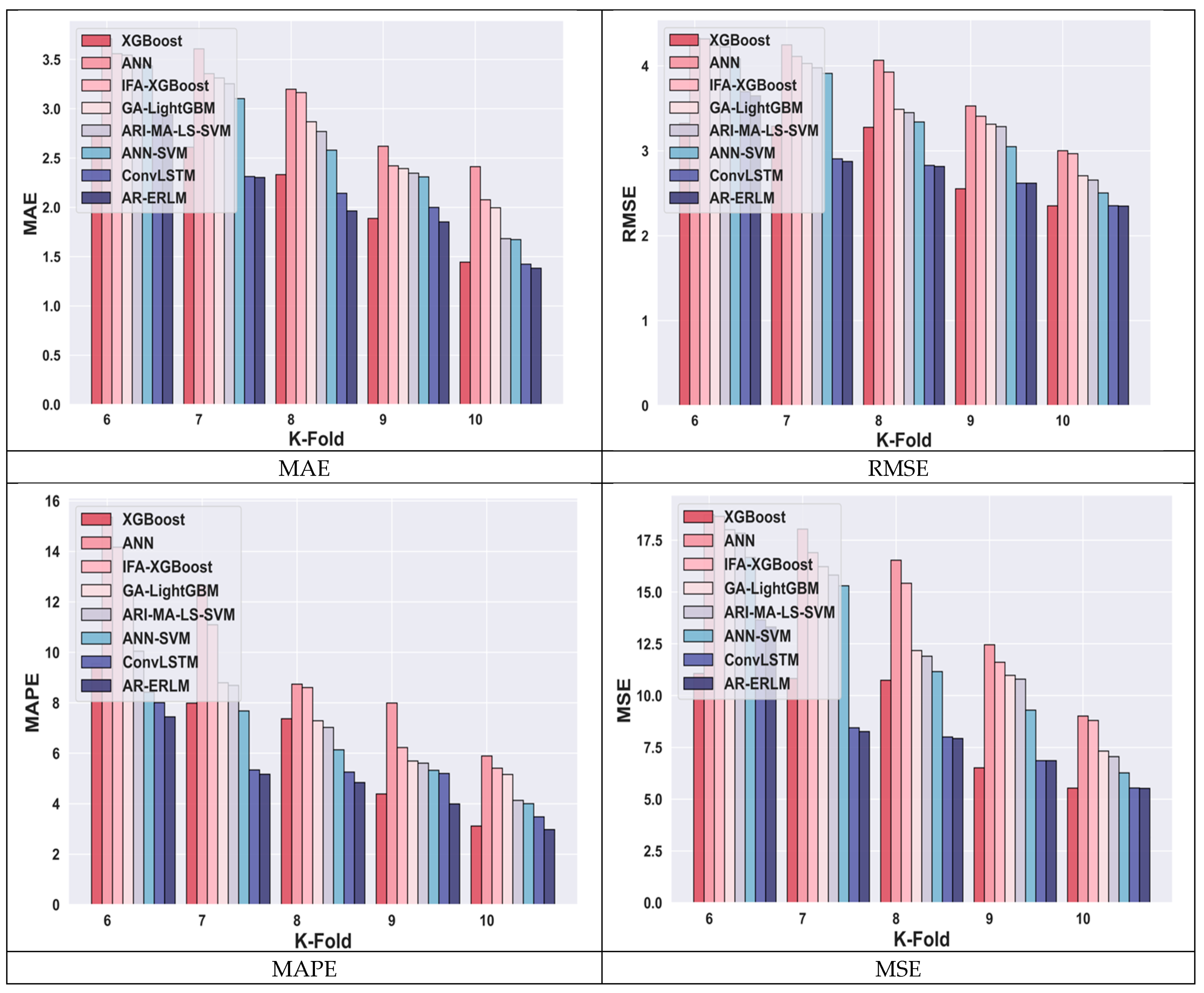
4.4.7. Comparative Analysis for Netflix Data Using k-Fold

The comparative analysis of the AR-ERLM model for predicting stock movements using Netflix data regarding metrics such as MAPE, MAE, RMSE, and MSE is delineated in Figure 9. For k-fold 10, the AR-ERLM model achieved an MAE of 1.51, which is notably lower than XGBoost by 0.05, ANN by 1.64, IFA-XGBoost by 0.79, GA-LightGBM by 0.71, ARI-MA-LS-SVM by 0.68, ANN-SVM by 0.33. Similarly, the RMSE measure for the AR-ERLM model is 2.43, showing an error difference of 0.01 over XGBoost, 1.27 over ANN, 0.59 over IFA-XGBoost, 0.44 over GA-LightGBM, 0.33 over ARI-MA-LS-SVM, 0.23 over ANN-SVM, and 0.08 over ConvLSTM. In terms of MSE, the AR-ERLM model outperforms other established techniques with a minimal value of 5.92, reduced over the existing technique XGBoost by 0.07, ANN by 7.83, IFA-XGBoost by 3.23, GA-LightGBM by 2.38, ARI-MA-LS-SVM by 1.73, ANN-SVM by 1.20, and ConvLSTM by 0.40. In terms of MAPE, the AR-ERLM model conquers a minimal value of 3.03, achieving an error difference of 0.89 over XGBoost, 3.87 over ANN, 2.13 over IFA-XGBoost, 0.74 over GA-LightGBM, 0.60 over ARI-MA-LS-SVM,0.48 over ANN-SVM, and 0.24 over ConvLSTM. These comparative results highlight the efficacy of the AR-ERLM model for stock movement prediction with minimal errors. Additionally, the model excels in capturing linear relationships and trends in time series data, while RNNs are adept at learning from sequential data due to their internal memory, making them suitable for recognizing patterns over time. Meanwhile, the gradient boosting technique effectively handles large datasets and enhances performance through its tree-based learning approach.

4.4.8. Comparative Analysis for Nifty50 Using k-Fold

The comparative evaluation of the AR-ERLM model with other existing methods for predicting stock movements using Nifty50 data, in terms of metrics MAPE, MAE, RMSE, and MSE, is illustrated in Figure 10. With k-fold 10, the AR-ERLM model gained an MAE score of 1.63, which is reduced over XGBoost by 0.23, ANN by 0.77, IFA-XGBoost by 0.48, GA- LightGBM by 0.27, ARI-MA-LS-SVM by 0.20, ANN-SVM by 0.17, and ConvLSTM by 0.10. Similarly, the RMSE for the AR-ERLM model is 2.45, outperforming the other competent techniques with the error difference of 0.27 over XGBoost, 0.57 over ANN, 0.50 over IFA-XGBoost, 0.30 over GA-LightGBM, 0.19 over ARI-MA-LS-SVM, 0.14 over ANN-SVM, and 0.13 over ConvLSTM. Subsequently, the AR-ERLM model attained the MSE score of 6.01, outperforming the other existing technique XGBoost by 1.39, ANN by 3.16, IFA-XGBoost by 2.72, GA-LightGBM by 1.56, ARI-MA-LS-SVM by 1.0, ANN-SVM by 0.75, and ConvLSTM by 0.66. For k-fold 10, the AR-ERLM model attains the minimal error of 2.70 for MAPE, exhibiting the error difference of 1.39 over XGBoost, 3.63 over ANN, 3.03 over IFA-XGBoost, 2.62 over GA-LightGBM, 1.74 over ARI-MA-LS-SVM, 0.81 over ANN-SVM, and 0.64 over ConvLSTM. From the comparative evaluation, the AR-ERLM model attained minimal errors for stock movement prediction due to its high potential in capturing the non-linear relationships and trends in complex time series data. Furthermore, the proposed approach attained low error values for the stock movement prediction and outperformed other baseline techniques utilized for comparison.

4.5. Comparative Discussion

Table 1. Comparative discussion of AR-ERLM using training percentage 90.

TP 90
Dataset/Methods	Metrics	XGBoost	ANN	IFA-XGBoost	GA-Light GBM	ARI-MA-LS-SVM	ANN-SVM	ConvLSTM	AR-ERLM
Meta Data	MAE	1.91	2.49	1.99	1.91	1.91	1.9	1.8	1.76
	RMSE	2.56	3.28	2.75	2.57	2.55	2.55	2.54	2.53
	MAPE	3.64	4.98	4.71	4.4	4.34	4.19	3.81	3.43
	MSE	6.55	10.78	7.57	6.65	6.55	6.55	6.53	6.43
Amazon Data	MAE	1.93	2.7	1.99	1.96	1.87	1.84	1.8	1.79
	RMSE	2.71	3.43	2.82	2.607	2.59	2.589	2.589	2.588
	MAPE	4.68	4.16	3.96	3.91	3.49	3.36	3.13	2.81
	MSE	7.36	11.8	8	6.79	6.71	6.72	6.71	6.70
Netflix Data	MAE	1.83	2.36	1.85	1.82	1.78	1.77	1.71	1.70
	RMSE	2.4	2.87	2.68	2.61	2.44	2.41	2.41	2.38
	MAPE	3.09	4.77	4.55	3.65	3.27	3.21	3.06	3.05
	MSE	5.79	8.26	7.20	6.84	5.96	5.81	5.78	5.66
Nifty50 Data	MAE	2.27	2.53	2.30	2.18	2.05	1.90	1.87	1.82
	RMSE	3.05	3.06	2.98	2.89	2.88	2.69	2.52	2.39
	MAPE	4.41	7.49	6.31	4.76	4.36	4.31	3.42	2.55
	MSE	9.30	9.36	8.86	8.37	8.28	7.22	6.37	5.72

demonstrates the comparative discussion of the AR-ERLM model with the other implemented techniques, such as GA-XGBoost, Conv-LSTM, XGBoost, ANN, and IFA-XGBoost. Stock movement prediction has gotten tremendous attention in recent times. However, stock prices are intrinsically complex, non-linear, and non-stationary; it is still challenging to make reliable predictions about the direction of stock prices. The existing methods employed for this task still face certain difficulties, such as overfitting issues, robustness, and data availability. To tackle these issues, this research presented an AR-ERLM model that incorporates the RNN, light GBM, and ARIMA statistical analysis. RNNs extract relevant features from historical data without manual intervention, and the Light GBM provides feature importance scores to aid in understanding which features contribute most to predictions. ARIMA captures linear dependencies in time series data, making it suitable for modeling stock prices that often exhibit trends and seasonality. Moreover, the proposed approach effectively handles the high dimensional data, minimizes the computation overload, extracts more significant features, and provides high prediction performance.

Table 2. Comparative discussion of AR-ERLM using k-fold 10.

k-Fold 10
Dataset/Methods	Metrics	XGBoost	ANN	IFA-XGBoost	GA-Light GBM	ARI-MA-LS-SVM	ANN-SVM	ConvLSTM	AR-ERLM
Meta Data	MAE	2.21	2.75	2.52	2.14	2.13	1.97	1.90	1.53
	RMSE	2.83	3.41	3.19	3.13	2.89	2.81	2.47	2.43
	MAPE	5.91	5.92	5.35	4.01	3.69	3.42	3.24	2.90
	MSE	8.04	11.65	10.18	9.82	8.37	7.90	6.12	5.93
Amazon Data	MAE	1.65	2.53	2.01	2.00	1.93	1.82	1.73	1.60
	RMSE	2.63	3.07	2.82	2.81	2.71	2.56	2.43	2.42
	MAPE	3.57	4.86	4.52	4.17	3.87	3.36	3.22	3.06
	MSE	6.91	9.42	7.96	7.91	7.36	6.57	5.88	5.88
Netflix Data	MAE	1.44	2.41	2.08	2.00	1.68	1.67	1.42	1.38
	RMSE	2.4	2.87	2.68	2.61	2.44	2.41	2.41	2.38
	MAPE	3.11	5.89	5.41	5.16	4.13	4.00	3.48	2.98
	MSE	2.36	3.00	2.97	2.71	2.66	2.50	2.35	2.34
Nifty50 Data	MAE	1.87	2.19	2.19	2.03	2.00	1.91	1.87	1.80
	RMSE	2.47	2.85	2.84	2.71	2.70	2.58	2.52	2.45
	MAPE	3.60	7.36	6.42	5.41	4.45	4.37	3.84	3.17
	MSE	6.09	8.13	8.07	7.34	7.30	6.66	6.35	6.01

illustrates the comparative discussion of AR-ERLM and other existing models using k-fold validation.

4.6. Ablation Study

The ablation study is carried out to examine the contribution of different components, including the ARIMA, RNN, and LightGBM, to the improvement of the AR-ERLM model. Further, the performance of the AR-ERLM and the individual models is examined, and the results are depicted in Figure 11. From Figure 11, the proposed AR-ERLM model achieved the minimum MSE score of 6.70, which is lower than ARIMA by 1.26, RNN by 1.55, and LightGBM by 3.83. More specifically, the proposed AR-ERLM model integrates the advantages of ARIMA, RNN, and Light GBM model and reduces the error in the prediction. In addition, the proposed model combines the ARIMA, RNN, and Light GBM and excels in identifying linear correlations and trends in time series data. Specifically, the RNN assists in learning the sequential data because of the internal memory, which makes the model appropriate for identifying patterns across time. Further, this observation explicates that the AR-ERLM possesses greater potential to predict the stock movement price compared to other individual models. Moreover, the ablation study analyzes the contribution of different components, including the ARIMA, RNN, and LightGBM, in the AR-ERLM model for improving stock movement prediction.

4.7. Diebold–Mariano Test

In this research, the Diebold–Mariano (DM) test is conducted to evaluate the predictive ability of different prediction models concerning their prediction error sequences. With the application of a series of statistical tests, the DM test assesses whether there is a substantial difference in the prediction capacity of the models under examination. Because of this, the DM test serves as an effective tool to assess the efficiency of various stock movement forecasting models prediction in the future. Further, the DM test to assess the performance is expressed as follows:

$$D{M}_{12}={\displaystyle \frac{{\overline{D}}_{12}}{{\sigma }_{D_{12}}}}$$

(25)

$$D_{12}={\displaystyle \frac{1}{P}}{\displaystyle \sum _{i=1}^P\left({\left(e_{it+1}^{\left(1\right)}\right)}^2-{\left(e_{it+1}^{\left(2\right)}\right)}^2\right)}$$

(26)

where $P$ indicates the stock index price, $D_{12}$ denotes the out-of-sample difference in the MSE between two prediction models, ${\overline{D}}_{12}$ indicates the mean of $D_{12}$, and ${\sigma }_{D_{12}}$ represents the standard deviation of $D_{12}$. Further, ${\left(e_{it+1}^{\left(1\right)}\right)}^2$ and ${\left(e_{it+1}^{\left(2\right)}\right)}^2$ represent the prediction errors of the two prediction models for flow I respectively. When the value of $DM$ is less than 0, it indicates that model 1 carries out the prediction better than model 2.

Table 3. Diebold–Mariano test.

Model	ARIMA	RNN	LightGBM
ARIMA	-	−0.854	−7.346
RNN	0.000	-	−8.976
LightGBM	0.000	−0.275	-

depicts the Diebold–Mariano test carried out for the different models utilized in the prediction.

4.8. Statistical Results

The statistical results obtained with the stock data and the Technical indicators for the Nifty50 data points are shown in

Table 4. Statistical results.

S. No	Stock Data			Technical Indicators
	Best	Mean	Variance	Best	Mean	Variance
1	82,100	16,436.41	7.32 × 108	82,100	5292.3	2.05 × 108
2	77,700	15,813.91	6.51 × 108	77,700	5155.382	1.84 × 108
3	84,500	16,794.48	7.77 × 108	84,500	5377.683	2.16 × 108
4	101,900	19,326.21	1.15 × 109	101,900	5937.903	3.12 × 108
5	118,200	21,685.12	1.57 × 109	118,200	6455.745	4.18 × 108
6	172,800	29,384.55	3.44 × 109	172,800	8134.185	8.89 × 108
7	164,100	28,076.77	3.1 × 109	164,100	7843.107	8.02 × 108
8	143,800	25,233.83	2.36 × 109	143,800	7223.883	6.16 × 108
9	148,000	25,866.29	2.5 × 109	148,000	7621.368	6.51 × 108
10	103,200	19,484.65	1.18 × 109	103,200	6227.626	3.18 × 108
11	129,600	23,267.16	1.9 × 109	129,600	7055.614	5 × 108
12	146,100	25,606.84	2.43 × 109	146,100	7402.419	6.36 × 108
13	232,100	37,989.47	6.29 × 109	232,100	10,115.53	1.61 × 109
14	176,000	30,000.12	3.57 × 109	176,000	8373.068	9.22 × 108
15	125,400	22,800.46	1.77 × 109	125,400	6807.859	4.69 × 108
16	158,700	27,607.59	2.88 × 109	158,700	7873.989	7.5 × 108
17	185,900	31,540.09	3.99 × 109	185,900	8734.912	1.03 × 109
18	175,500	30,072.63	3.54 × 109	175,500	8421.444	9.17 × 108
19	191,200	32,360.76	4.22 × 109	191,200	8940.341	1.09 × 109
20	192,000	32,504.62	4.25 × 109	192,000	8983.887	1.1 × 109
21	185,100	31,539.45	3.95 × 109	185,100	8784.664	1.02 × 109
22	256,300	41,711.68	7.69 × 109	256,300	11,016.64	1.96 × 109
23	267,300	43,268.17	8.38 × 109	267,300	11,360.65	2.13 × 109
24	210,100	35,041.69	5.12 × 109	210,100	9570.6	1.31 × 109
25	208,700	34,834.81	5.05 × 109	208,700	9535.426	1.3 × 109

. Further, the statistical test is carried out to find the significant difference between the data points and ensure the robustness of the results.

5. Conclusions

In conclusion, this research proposes an ensemble method that leverages the benefits of the statistical analysis model with the RNN and LightGBM. Stock market predictions always carry inherent uncertainty, and combining multiple models can provide a more robust approach to forecasting. By using the proposed AR-ERLM model, traders can make informed decisions about buying or selling stocks. Furthermore, the proposed model is computationally efficient and can handle large datasets with minimal memory usage. It also combines the strengths of decision trees and gradient boosting, resulting in accurate predictions. Additionally, the technical indicators employed in this research aid in determining the direction of trends and provide more statistical parameters for evaluation. The performance of the AR-ERLM model for stock movement prediction is compared with other implemented methods, and the outcomes show that the proposed framework achieves lower errors with MSE 4.45, RMSE 2.35, and MAE 1.58. Moreover, the implementation results ensure the practical application of the AR-ERLM model for predicting stock price movement and offer investors greater decision support to adjust their investment strategies for maximizing profit and lowering the risks associated with margin trading. Even though most of the stock prices have a daily pattern, as in the proposed approach, this can be changed in other areas due to the seasonal pattern on some sales datasets. Hence, an attempt will be made to utilize diverse lengths of historical data and other significant features, including the exchange rates and other macroeconomic indicators in the future.

References

1. Patel, M.; Jariwala, K.; Chattopadhyay, C. A Hybrid Relational Approach Towards Stock Price Prediction and Profitability. IEEE Trans. Artif. Intell. 2024, 5, 5844–5854. [Google Scholar] [CrossRef]
2. Bezerra, P.C.S.; Albuquerque, P.H.M. Volatility forecasting via SVR–GARCH with mixture of Gaussian kernels. Comput. Manag. Sci. 2017, 14, 179–196. [Google Scholar] [CrossRef]
3. Nti, I.K.; Adekoya, A.F.; Weyori, B.A. A systematic review of fundamental and technical analysis of stock market predictions. Artif. Intell. Rev. 2020, 53, 3007–3057. [Google Scholar] [CrossRef]
4. Ahmadi, E.; Jasemi, M.; Monplaisir, L.; Nabavi, M.A.; Mahmoodi, A.; Jam, P.A. New efficient hybrid candlestick technical analysis model for stock market timing on the basis of the Support Vector Machine and Heuristic Algorithms of Imperialist Competition and Genetic. Expert Syst. Appl. 2018, 94, 21–31. [Google Scholar] [CrossRef]
5. Lin, Y.; Liu, S.; Yang, H.; Wu, H. Stock trend prediction using candlestick charting and ensemble machine learning techniques with a novelty feature engineering scheme. IEEE Access 2021, 9, 101433–101446. [Google Scholar] [CrossRef]
6. Saetia, K.; Yokrattanasak, J. Stock movement prediction using machine learning based on technical indicators and Google trend searches in Thailand. Int. J. Financ. Stud. 2022, 11, 5. [Google Scholar] [CrossRef]
7. Khan, W.; Ghazanfar, M.A.; Azam, M.A.; Karami, A.; Alyoubi, K.H.; Alfakeeh, A.S. Stock market prediction using machine learning classifiers and social media, news. J. Ambient. Intell. Humaniz. Comput. 2022, 13, 3433–3456. [Google Scholar] [CrossRef]
8. Peng, Y.; Albuquerque, P.H.M.; Kimura, H.; Saavedra, C.A.P.B. Feature selection and deep neural networks for stock price direction forecasting using technical analysis indicators. Mach. Learn. Appl. 2021, 5, 100060. [Google Scholar] [CrossRef]
9. Ayala, J.; García-Torres, M.; Noguera, J.L.V.; Gómez-Vela, F.; Divina, F. Technical analysis strategy optimization using a machine learning approach in stock market indices. Knowl.-Based Syst. 2021, 225, 107119. [Google Scholar] [CrossRef]
10. Jiang, J.; Wu, L.; Zhao, H.; Zhu, H.; Zhang, W. Forecasting movements of stock time series based on hidden state guided deep learning approach. Inf. Process. Manag. 2023, 60, 103328. [Google Scholar] [CrossRef]
11. Chen, W.; Zhang, H.; Mehlawat, M.K.; Jia, L. Mean–variance portfolio optimization using machine learning-based stock price prediction. Appl. Soft Comput. 2021, 100, 106943. [Google Scholar] [CrossRef]
12. Fabozzi, F.J.; Markowitz, H.M.; Gupta, F. Portfolio selection. Handb. Financ. 2008, 2, 3–13. [Google Scholar]
13. Yun, K.K.; Yoon, S.W.; Won, D. Prediction of stock price direction using a hybrid GA-XGBoost algorithm with a three-stage feature engineering process. Expert Syst. Appl. 2021, 186, 115716. [Google Scholar] [CrossRef]
14. Jiang, L.C.; Subramanian, P. Forecasting of stock price using autoregressive integrated moving average model. J. Comput. Theor. Nanosci. 2019, 16, 3519–3524. [Google Scholar] [CrossRef]
15. Koki, C.; Leonardos, S.; Piliouras, G. Exploring the predictability of cryptocurrencies via Bayesian hidden Markov models. Res. Int. Bus. Financ. 2022, 59, 101554. [Google Scholar] [CrossRef]
16. Dong, S.; Wang, J.; Luo, H.; Wang, H.; Wu, F.X. A dynamic predictor selection algorithm for predicting stock market movement. Expert Syst. Appl. 2021, 186, 115836. [Google Scholar] [CrossRef]
17. Wang, C.; Chen, Y.; Zhang, S.; Zhang, Q. Stock market index prediction using deep Transformer model. Expert Syst. Appl. 2022, 208, 118128. [Google Scholar] [CrossRef]
18. Tao, Z.; Wu, W.; Wang, J. Series decomposition Transformer with period-correlation for stock market index prediction. Expert Syst. Appl. 2024, 237, 121424. [Google Scholar] [CrossRef]
19. Ronaghi, F.; Salimibeni, M.; Naderkhani, F.; Mohammadi, A. COVID19-HPSMP: COVID-19 adopted Hybrid and Parallel deep information fusion framework for stock price movement prediction. Expert Syst. Appl. 2022, 187, 115879. [Google Scholar] [CrossRef]
20. Amazon Dataset. Available online: https://finance.yahoo.com/quote/AMZN (accessed on 2 May 2024).
21. Meta Dataset. Available online: https://finance.yahoo.com/quote/META (accessed on 2 May 2024).
22. Netflix Dataset. Available online: https://finance.yahoo.com/quote/NFLX (accessed on 2 May 2024).
23. Ouyang, Y.; Li, S.; Yao, K.; Wang, J. Analysis of Investment Indicators for the Electronic Components Sector of the A-Share Market. In Proceedings of the 2022 International Conference on Bigdata Blockchain and Economy Management (ICBBEM 2022), Guangzhou, China, 26–28 August 2022; Atlantis Press: Paris, France, 2022; pp. 180–186. [Google Scholar]
24. Joshi, D.L. Use of Moving Average Convergence Divergence for Predicting Price Movements. Int. Res. J. MMC (IRJMMC) 2022, 3, 21–25. [Google Scholar] [CrossRef]
25. Chandrika, P.V.; Srinivasan, K.S.; Taylor, G. Predicting stock market movements using artificial neural networks. Univers. J. Account. Financ. 2021, 9, 405–410. [Google Scholar] [CrossRef]
26. Wahyudi, S.T. The ARIMA Model for the Indonesia Stock Price. Int. J. Econ. Manag. 2017, 11, 223–236. [Google Scholar]
27. Zhang, G.P. Time series forecasting using a hybrid ARIMA and neural network model. Neurocomputing 2003, 50, 159–175. [Google Scholar] [CrossRef]
28. Gan, M.; Pan, S.; Chen, Y.; Cheng, C.; Pan, H.; Zhu, X. Application of the machine learning lightgbm model to the prediction of the water levels of the lower columbia river. J. Mar. Sci. Eng. 2021, 9, 496. [Google Scholar] [CrossRef]
29. Ke, G.; Meng, Q.; Finley, T.; Wang, T.; Chen, W.; Ma, W.; Ye, Q.; Liu, T.Y. Lightgbm: A highly efficient gradient boosting decision tree. Adv. Neural Inf. Process. Syst. 2017, 30. [Google Scholar]
30. Zhao, X.; Liu, Y.; Zhao, Q. Cost Harmonization LightGBM-Based Stock Market Prediction. IEEE Access 2023, 11, 105009–105026. [Google Scholar] [CrossRef]
31. Selvin, S.; Vinayakumar, R.; Gopalakrishnan, E.A.; Menon, V.K.; Soman, K.P. Stock price prediction using LSTM, RNN and CNN-sliding window model. In Proceedings of the 2017 international conference on advances in computing, communications and informatics (ICACCI), Udupi, India, 13–16 September 2017; pp. 1643–1647. [Google Scholar]
32. Nifty50 Dataset. Available online: https://finance.yahoo.com/quote/%5ENSEI/history/?fr=sycsrp_catchall (accessed on 22 February 2025).
33. Huang, C.; Cai, Y.; Cao, J.; Deng, Y. Stock complex networks based on the GA-LightGBM model: The prediction of firm performance. Inf. Sci. 2024, 700, 121824. [Google Scholar] [CrossRef]
34. Xiao, C.; Xia, W.; Jiang, J. Stock price forecast based on combined model of ARI-MA-LS-SVM. Neural Comput. Appl. 2020, 32, 5379–5388. [Google Scholar] [CrossRef]
35. Ali, M.; Khan, D.M.; Aamir, M.; Ali, A.; Ahmad, Z. Predicting the direction movement of financial time series using artificial neural network and support vector machine. Complexity 2021, 2021, 2906463. [Google Scholar] [CrossRef]
Figure 1. Flow diagram of the AR-ERLM model for stock movement prediction.
Systems 13 00162 g001
Figure 2. AR-ERLM model architecture combining the ARIMA statistical analysis technique for feature extraction and the LightGBM and RNN techniques for prediction.
Systems 13 00162 g002
Figure 3. Comparative analysis for Meta data using training percentage analysis.
Systems 13 00162 g003
Figure 4. Comparative analysis of Amazon data using training percentage analysis.
Systems 13 00162 g004
Figure 5. Comparative analysis of Netflix data using training percentage analysis.
Systems 13 00162 g005
Figure 6. Comparative analysis of Nifty50 data using training percentage analysis.
Systems 13 00162 g006
Figure 7. Comparative analysis of Meta data using k-fold.
Systems 13 00162 g007
Figure 8. Comparative analysis of Amazon data using k-fold.
Systems 13 00162 g008
Figure 9. Comparative analysis of Netflix data using k-fold.
Systems 13 00162 g009
Figure 10. Comparative analysis of Nifty50 data using k-fold.
Systems 13 00162 g010
Figure 11. Ablation study.
Systems 13 00162 g011