Article

Optimal Delay Product Differentiation System Under the Cap-and-Trade Environment

by
Shouyao Xiong
* and
Liu Yang
School of Mathematics and Statistics, Changsha University of Science and Technology, Changsha 410104, China
*
Author to whom correspondence should be addressed.
Systems 2025, 13(3), 161; https://doi.org/10.3390/systems13030161
Submission received: 8 January 2025 / Revised: 17 February 2025 / Accepted: 20 February 2025 / Published: 26 February 2025
(This article belongs to the Section Supply Chain Management)

Abstract

:
Delayed product differentiation (DD) is a two-stage hybrid system that meets the dual demands of multiple product types and fast response times. This paper studies the optimal production planning problem for DD systems under a cap-and-trade environment. We establish a model to minimize the total cost of storage, late delivery penalties, and emission quota trading and make optimal decisions on inventory levels, emission trading quantities, and types of emission trading. Data analyses show that the introduction of carbon cap-and-trade policies can effectively optimize the optimal inventory of the DD system. The loading in the MTS and MTO stages has an asymmetric impact on the cost and emission advantages of DD. Under carbon cap-and-trade policies, DD is more available than a pure MTS system.

1. Introduction

An increasing number of people believe that carbon emissions from corporate activities are one of the main causes of global climate change. To ensure sustainable development for humanity in social, environmental, and economic aspects, many countries and regions have established various regulations for corporate activities. The cap-and-trade policy is one of the more popular regulations. Under the cap-and-trade system, companies receive a certain amount of initial emission allowances for a planning period and are allowed to trade emission permits with other companies or government agencies on the external market. The European Union’s Emissions Trading System (EU ETS) is the first and currently the world’s largest carbon trading system, accounting for the highest proportion of carbon trading volume. As of 2024, the EU ETS covers over 15,000 fixed installations and about 1500 aviation operators [1].
At the same time, the manufacturing industry is transitioning from Mass Production to Mass Customization to meet the growing demand for product diversity and personalization. The traditional Make-To-Stock (MTS) production system offers high responsiveness, but the storage costs associated with high inventory levels and potential carbon emissions pose significant challenges [2,3]. In contrast, the Make-To-Order (MTO) production system produces products based on specific customer orders, reducing inventory but resulting in longer production lead times [4,5,6]. Against this backdrop, the Delayed Differentiation (DD) system, as a hybrid model of MTS and MTO, provides a more flexible production approach and has demonstrated economic advantages in conventional settings [7,8,9,10,11].
However, under carbon policies, does the DD system still hold an advantage? Can it achieve both carbon reduction and cost optimization simultaneously? For analyzing the applicability of the DD system under carbon regulations, we compare it with the pure MTS system. By establishing a mathematical model, we examine the impact of loading each stage on costs, emissions, and carbon trading decisions under different production systems, aiming to provide theoretical support for manufacturers in selecting an appropriate production strategy under carbon constraints.

2. Literature Review

This work primarily relates to two streams of research. We will highlight how our research differs from these studies.
The first stream of research related to our work is delayed differentiation (DD). DD was proposed and studied in the early 21st century and carries several benefits. Jayashankar M et al. [12] use vanilla boxes as semi-finished products and model a two-stage integer program, applying DD to solve real-world problems. Gupta and Benjaafar et al. [13] establish a cost model based on service level constraints, using queuing theory to compare the cost levels of pure MTS systems and DD systems. They solve for the optimal semi-finished product buffer inventory. Building on Gupta’s research, Jewkes et al. [14] incorporate product characteristics into the manufacturer’s decision-making framework to analyze the impact of market characteristics on the differentiation point and the size of the semi-finished product buffer inventory. When there are replenishment costs, Eman et al. [15], based on Gupta’s model, introduce batch replenishment strategies into the MTS-MTO hybrid system to reduce the number of replenishments, making it more aligned with actual production. Su et al. [16] use a two-stage M/M/1 queuing model to compare pure MTO and configure-to-order (CTO) supply chain models, where CTO applies DD to the MTO system. The results show that DD improves MTO systems in terms of cost and customer waiting time. Wenhui Zhou et al. [17] research a two-stage queuing network with demand arriving according to the Markovian Arrival Process. They introduce the Markovian Process into delayed differentiation systems and study the impact of demand correlation on supply chain optimization based on the FP strategy. Fei Qingyi et al. [18] introduce process investment into a two-stage flexible production system and explore how investment levels affect delayed differentiation strategies, using customer order fulfillment delays and inventory risks as indicators. Dia Constantin Bandalya et al. [19] study delayed production systems for perishable products, integrating delayed decision-making and deterioration mitigation decisions into a single model and establishing a multi-period planning model with recourse.
The second related research stream is on the cap-and-trade policy. To study the impact of carbon policies on production costs and emissions, many articles incorporate the emissions trading price into their cost (profit) functions. They solve for the manufacturer’s optimal production decisions and the optimal quantity of emissions permits traded under the cap-and-trade mechanism. Based on whether the carbon trading price varies over time, we categorize these articles into two main groups. Additionally, for the category where the trading price does not vary over time, we further classify them based on whether the buying price and selling price are equal.
(i)
Unit emissions allowances sell price equals the purchase price
Bin Zhang et al. [20] study the multi-product production planning problem where the carbon price is an exogenous variable determined by the manufacturer. They model the profit function and investigate the optimal solution under profit maximization conditions. Kaiying Cao et al. [21] consider manufacturers selling green products under both the cap-and-trade policy (CTP) and the low carbon subsidy policy (LCSP). They determine the optimal solution under conditions where the government commits to maximizing social welfare, and the manufacturer pursues maximal profit. Hu, BY et al. [22] study a dual-product MTO supply chain, where manufacturers reduce carbon emissions by investing in emission reduction technologies. They compare the profits and carbon emissions under decentralized and centralized decision-making, finding that decentralized decision-making is more advantageous.
(ii)
Unit emissions allowances purchase and sell prices are unequal
Ping He et al. [23] study the production batch problem based on the EOQ model, comparing the effects of the taxation policy and the cap and trade policy on profit and carbon emissions. They find that both policies lead to the same optimal carbon emissions. Xiaoping Xu et al. [24] investigate the production and pricing issues in a dual-product MTO supply chain, comparing the output of regular products and green products. They find that the cap-and-trade policy does not strongly incentivize manufacturers to produce low-carbon products. Shouyao Xiong et al. [25] study the optimal production planning problem for a single-product hybrid MTS/MTO system, finding that optimal production decisions and carbon trading decisions are significantly influenced by the initial emission allowances.
(iii)
Unit emissions allowances trade price is stochastic
Xiting Gong et al. [26] construct a dynamic programming model for the single-product problem of minimizing the expected total discounted cost. The manufacturer can choose between a green and a regular production technology, with the carbon trading price determined by a stochastic forward contract price. The study finds that when firms trade quotas or use both production technologies simultaneously, the optimal base stock level depends solely on the trading price. In other scenarios, the optimal base stock level also depends on initial inventory and quota levels. Baiyun Yuan et al. [27] use discrete-time optimal control theory to study the multi-period production problem for manufacturers in a low-carbon environment. They establish an inter-temporal optimization model aiming to maximize total net profit and solve and compare the optimal CER purchase quantities, carbon trading quantities, and emission reduction strategies for each period.
Our study is also associated with most of the papers on hybrid MTS/MTO and semi-finished goods production, and we provide Table 1 that summarizes the differences between some of the studies that are closely related to our work.
Our work differs from the above-mentioned studies in that we explore a novel intersection by integrating two-stage delayed differentiation (DD) with carbon cap and trade policies. Unlike existing literature that primarily focuses on either DD optimization or carbon trading strategies separately, our research investigates how DD systems can strategically optimize production decisions alongside carbon emission trading under regulatory frameworks. By examining the synergistic effects of DD’s production flexibility and the dynamic nature of carbon pricing mechanisms, this study aims to propose optimal strategies that balance economic efficiency with environmental sustainability within the context of carbon policy implementations.

3. Model

3.1. Model Description

We consider a manufacturing system with two production stages, where the final product comes in M types. We will compare two different production control systems: a pure MTS (Make-to-Stock) system and a system with DD (Delayed Differentiation). In the pure MTS system, the final products are produced and stored as inventory to buffer against demand. In the system with DD, semi-finished products are produced and stored as inventory, while the final products are made to order. The general processes of the DD system and the pure MTS system are presented through Figure 1.
Under the carbon trading policy, the comparison between the pure MTS system and the system with DD focuses on two main aspects: base cost and service level. The base cost primarily includes emissions trading-related costs, storage costs, and backorder costs (excluding production costs, see references [16]). An acceptable service level can be defined as the upper limit of the average order fulfillment time. However, for the DD system, it is assumed customers can tolerate a certain level of delay, as this production system cannot deliver products immediately. The objective of the manufacturing system is to minimize the base cost within a production cycle based on a fixed service level.
At the start of the production planning period, the manufacturer receives z 0 units emission allowances and makes production decisions and emissions trading decisions. During the production planning stage, demand for product-j ( j = 1 , , M ) follows a Poisson process with rate λ j , the total demand rate denotes as  Λ .
We assumed that the emissions in the system mainly come from production and storage. The emissions per unit of product are independent of the product type, and the emissions from producing a unit of product in stage-1 are higher than those in stage-2. Additionally, the emissions from storing a finished product are higher than those from storing a semi-finished product. Since the work-in-progress levels of the two systems are roughly the same, we do not consider the carbon emissions from the production and storage of work-in-progress [13]. At the end of a production cycle, the manufacturer must ensure that the balance of the allowances account is non-negative or otherwise be liable for a penalty π per unit.
In both systems, inventory management is based on a basic stock policy, meaning that each incoming demand triggers a raw material package to enter the stage-1 queue. The base inventory level for semi-finished goods is denoted as s d , and the basic inventory level for finished goods is denoted as s t . The processing efficiency at stage-i (i = 1, 2) is defined as μ i , let  Λ / μ i = ρ i , where ρ i represents the loading rate at stage-i (i = 1, 2). It is assumed that the processing times per unit at each stage follow an exponential distribution.
For a pure MTS system, demand is prioritized to be met by inventory. If the corresponding finished goods inventory is depleted, subsequent orders are backordered. For a system with DD, each demand arrival triggers the delivery of a semi-finished product from inventory to the differentiated stage, which is then added to the stage-2 job queue to await differentiation. However, when the semi-finished goods inventory is empty, demand will be backlogged in stage-1 for processing.
Below is a summary of the notation used in the paper:
  • D j max maximum demand for product-j in a single production period
  • V t the summary cost in the MTS system.
  • V d the summary cost in the DD system.
  • C t the total emissions in the MTS system.
  • C d the total emissions in the DD system.
  • s d the base stock level for the semi-finished product in the DD system (decision variable).
  • s t the base stock level for the finished product (decision variable).
  • z 0 the initial emission allowances in the system.
  • z t Emissions allowances after trading decisions in pure MTS (decision variable).
  • z d Emissions allowances after trading decisions in DD (decision variable).
  • μ Emissions allowances purchase price.
  • v Emissions allowances sale price.
  • h t the unit finished product storage cost.
  • h d semi-finished product storage cost per unit.
  • π penalty cost for excess emissions per unit.
  • μ i the processing rate at stage-i.
  • ρ i the stage-i loading, Λ / μ i = ρ i .
  • Λ the rate of total demand.
  • I ¯ t ( s t ) the expected inventory of finished product in the pure MTS system.
  • I ¯ d ( s d ) the expected inventory of semi-finished product in the DD system.
  • B ¯ d ( s d ) the expected backorders of semi-finished product in the DD system.
  • B ¯ t ( s t ) the expected backorders of finished product in the pure MTS system.
  • F ¯ d ( s d ) the order-fulfillment time in the DD system.
  • F ¯ t ( s t ) the order-fulfillment time in the pure MTS system.
  • λ j the rate of a Poisson process that demand for product-j occurs.
  • c 1 the emissions of producing unit product in stage-1.
  • c 2 the emissions of producing unit product in stage-2.
  • c 3 the emissions of storing unit finished product.
  • c 4 the emissions of storing unit semi-finished product.
  • α the lead time of unit customer order.

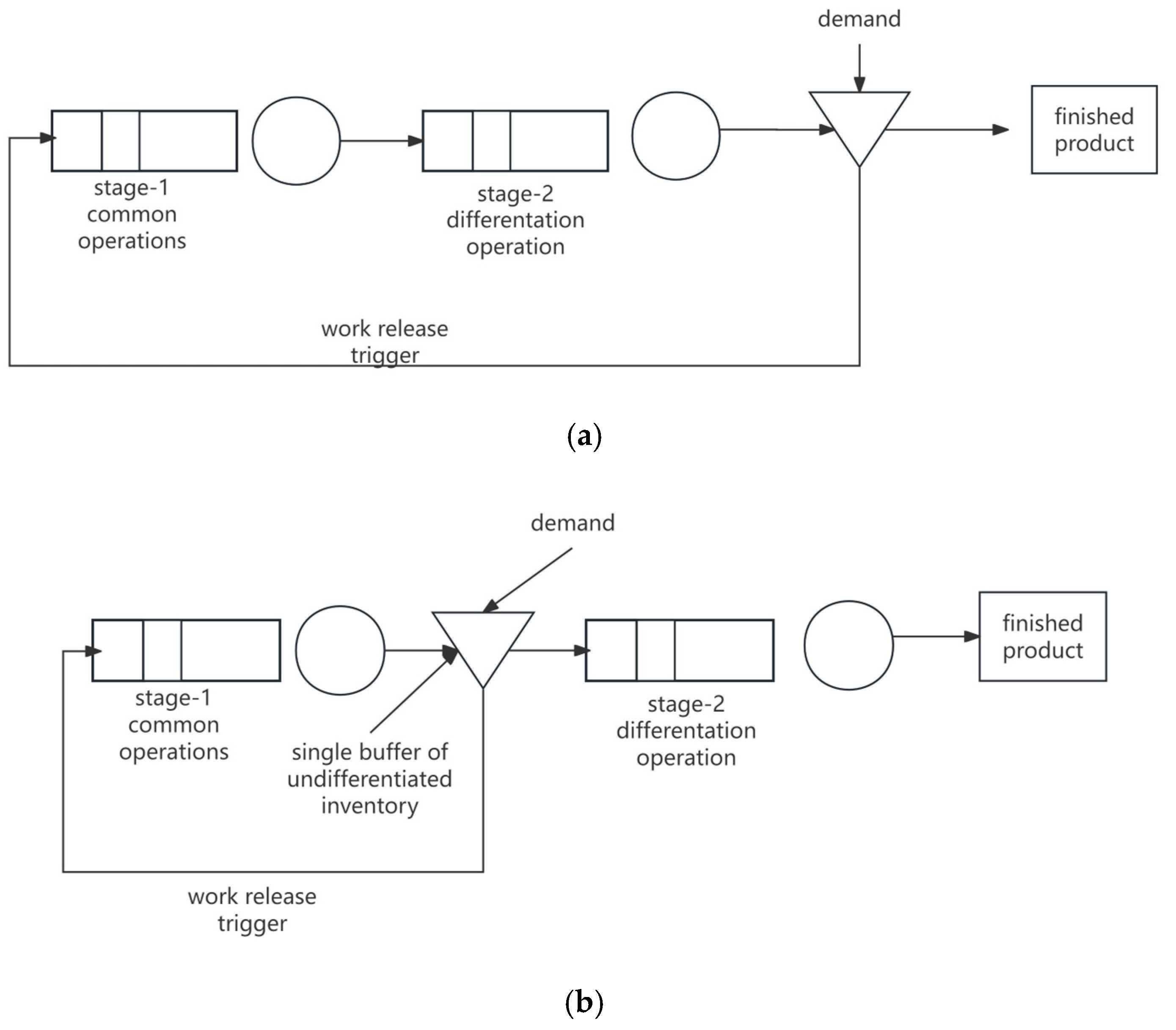
3.2. Pure Make-to-Stock System

In the pure MTS system, since demand is Poisson and processing times are exponentially distributed the two stations behave like M / M / 1 queues in tandem. Therefore, the expected inventory, backorder level, and order-fulfillment time are:
I ¯ t ( s t ) = M ( s t ( 1 + ρ ^ s t + 1 ) 2 ρ ^ ( 1 ρ ^ s t ) 1 ρ ^ ) if   ρ 1 = ρ 2 = ρ , M 2 ( 1 ρ 1 ) ( 1 ρ 2 ) ( ρ 2 ρ 1 ) ( s t ρ ^ 2 ( 1 ρ ^ 2 ) ρ ^ 2 2 ( 1 ρ ^ 2 s t ) ( 1 ρ ^ 2 ) 2 s t ρ ^ 1 ( 1 ρ ^ 1 ) ρ ^ 1 2 ( 1 ρ ^ 1 s t ) ( 1 ρ ^ 1 ) 2 ) otherwise ,
F ¯ t ( s t ) = M Λ ( s t ρ ^ s t + 1 + 2 ρ ^ s t + 1 1 ρ ^ ) if   ρ 1 = ρ 2 = ρ , M 2 ( 1 ρ 1 ) ( 1 ρ 2 ) Λ ( ρ 2 ρ 1 ) ( ρ ^ 2 s t + 2 ( 1 ρ ^ 2 ) 2 ρ ^ 1 s t + 2 ( 1 ρ ^ 1 ) 2 ) otherwise ,
B ¯ f ( b f ) = I ¯ f ( b f ) + M ( ρ ^ 1 1 ρ ^ 1 + ρ ^ 2 1 ρ ^ 2 b f ) ,
where ρ ^ = ρ / [ M ( 1 ρ ) + ρ ] , and ρ ^ i = ρ i / [ M ( 1 ρ i ) + ρ i ] .

3.2.1. Emissions Trading Cost

μ ( z t z 0 ) + ν [ ( z t z 0 ) ] + ,

3.2.2. Inventory Cost

h t I ¯ t ( s t ) ,

3.2.3. Penalty Cost for Backorders

b B ¯ t ( s t ) ,

3.2.4. Penalty Cost for the Excess Emissions

  • MTS stage-1 emissions:
c 1 s t + j = 1 M k j = 0 D j max k j p t ( k j ) ,
  • MTS stage-2 emissions:
c 2 s t + j = 1 M k j = 0 D j max k j p t ( k j ) ,
  • Inventory emissions:
c 3 I ¯ t ( s t ) .
Total emissions:
C t = c 1 s t + j = 1 M k j = 0 D j max k j p t ( k j ) + c 2 s t + j = 1 M k j = 0 D j max k j p t ( k j ) + c 3 I ¯ t ( s t ) ,
The penalty cost for the excess emissions:
π C t z t + .

3.2.5. MTS Summary

V t = μ ( z t z 0 ) + ν [ ( z t z 0 ) ] + + h t I t ( s t ) + b B ¯ t ( s t ) + π C t z t + , ( x ) + means   the   non - negative   part ,   i . e . ,   max ( 0 , x ) .
The optimization problem:
min V t s t . F ¯ t ( s t ) < α .

3.3. Delayed Differentiation System

In the system with DD, calculating the above metrics is more difficulted, because there is a positive correlation between the arrivals of undifferentiated units, when these units move from stage-1 to stage-2 when 0 < s d < . The steady-state probabilities cannot be calculated using the product-form structure of the serial M/M/1 queues. To simplify the analysis and modeling process of the system, we approximate the inter-arrival times of units at stage-2 to follow an exponential distribution, thus treating it as an M/M/1 queue [13]. Below are expressions for the expected inventory level, backorders level with the order fulfillment time in the system with DD:
I ¯ d ( s d ) = s d ( ρ 1 ( 1 ρ 1 s d ) 1 ρ 1 ) ,
B ¯ d ( s d ) ρ 2 1 ρ 2 + ρ 1 s d + 1 1 ρ 1 ,
F ¯ d ( s d ) ρ 1 s d + 1 Λ ( 1 ρ 1 ) + ρ 2 Λ ( 1 ρ 2 ) .

3.3.1. Emissions Trading Cost

μ ( z d z 0 ) + ν [ ( z d z 0 ) ] + .

3.3.2. Inventory Cost

h d I ¯ d ( s d ) .

3.3.3. Penalty Cost for Backorders

b B ¯ d ( s d ) .

3.3.4. Penalty Cost for the Excess Emissions

  • Stage-1 manufacturing emissions:
    c 1 s d + k j = 0 D j max k j p d ( k j ) ;
  • Stage-2 manufacturing emissions:
    c 2 k j = 0 D j max k j p d ( k j ) ;
  • Inventory emissions:
    c 4 I ¯ d ( s d ) .
  • Total emissions:
    C d = c 1 s d + k j = 0 D j max k j p d ( k j ) + c 2 k j = 0 D J max k j p d ( k j ) + c 4 I ¯ d ( s d ) ,
  • The penalty cost for the excess emissions is
    π C d z d + .

3.3.5. DD Summary

V d = μ ( z d z 0 ) + ν [ ( z d z 0 ) ] + + h d I ¯ d ( s d ) + b B ¯ d ( s d ) + π C d z d + .
The optimization problem:
min V d s t . F ¯ d ( s d ) < α .

4. Optimal Policies

Before the optimal system cost and the optimal emissions trading decisions can be calculated, we need to determine the optimal base stock levels. Therefore, in the following formulas, we represent the optimal base stock levels with s t * , s d * . To study the mechanism of carbon trading policies in depth, we assume that manufacturers will definitely engage in carbon trading, i.e., π > μ > v .

4.1. Production Decisions and Emissions Decisions in the Pure MTS System

Theorem 1.
During the planning period, the optimal emissions trading quantity is as follows:
z * t = C t z t z 0 C t z t < z 0 ,
A proof can be found in Appendix A.
Theorem 2.
Since the equation has no explicit solution,  s t *  is defined by the following equation:
(1) 
If  z t z 0 ,  s t *  is obtained from the following equation:
V t s t = μ ( C t z 0 ) + h t I ¯ t ( s t ) + b B ¯ t ( s t ) s t = 0 ;
(2) 
If  z t < z 0 ,  s t *  is obtained from the following equation:
V t s t = v ( z 0 C t ) + h t I ¯ t ( s t ) + b B ¯ t ( s t ) s t = 0
An explanation can be found in Appendix B.
Theorem 3.
(1) 
If  z t z 0 , means that the manufacturer needs to purchase emissions allowances; the minimum cost for the manufacturer is:
V t * = μ ( z t * z 0 ) + h t I ¯ t ( s t * ) + b B ¯ t ( s t * ) ;
(2) 
If  z t < z 0 , means the manufacturer needs to sell emissions allowances; the minimum cost for the manufacturer is:
V t * = v ( z 0 z t * ) + h t I ¯ t ( s t * ) + b B ¯ t ( s t * ) ,
An explanation can be found in Appendix B.

4.2. Production Decisions and Emissions Decisions in the DD System

Theorem 4.
In the DD system, the optimal emissions trading quantity is as follows:
z * d = C d z d z 0 0 z 0 ( c 1 + c 2 ) k j = 0 D j max k j p d ( k j ) + c 1 s d * + c 4 I ¯ d ( s d * ) C d z d < z 0 ( c 1 + c 2 ) k j = 0 D j max k j p d ( k j ) + c 1 s d * + c 4 I ¯ d ( s d * ) < z 0 ,
Theorem 5.
The optimal inventory level obtained under the cost minimization condition for the system with DD is as follows:
(1) 
If  z d z 0
s d * = ln h d + μ ( c 1 + c 4 ) ( ρ 1 1 ) b ρ 1 ln ρ 1 + h d ρ 1 ln ρ 1 ρ 1 1 + c 4 μ ρ 1 ln ρ 1 ρ 1 1 / ln ρ 1 ,
(2) 
If  z d < z 0
s d * = ln h d + v ( c 1 + c 4 ) ( ρ 1 1 ) b ρ 1 ln ρ 1 + h d ρ 1 ln ρ 1 ρ 1 1 + c 4 v ρ 1 ln ρ 1 ρ 1 1 / ln ρ 1 ,
An explanation can be found in Appendix D.
Theorem 6.
(1) 
if z d z 0 , means that the manufacturer needs to purchase emissions allowances; the minimum cost for the manufacturer is:
V d * = μ ( ( c 1 + c 2 ) ρ 1 1 ρ 1 + c 1 s d * + c 4 s d * ( ρ 1 ( 1 ρ 1 s d * ) 1 ρ 1 ) z 0 ) + h d s d * ( ρ 1 ( 1 ρ 1 s d * ) 1 ρ 1 ) + b ρ 2 1 ρ 2 + ρ 1 s d * + 1 1 ρ 1 ;
(2) 
if  z d < z 0 , means that the manufacturer needs to purchase emissions allowances; the minimum cost for the manufacturer is:
V d * = v ( ( c 1 + c 2 ) ρ 1 1 ρ 1 + c 1 s d * + c 4 s d * ( ρ 1 ( 1 ρ 1 s d * ) 1 ρ 1 ) z 0 ) + h d s d * ( ρ 1 ( 1 ρ 1 s d * ) 1 ρ 1 ) + b ρ 2 1 ρ 2 + ρ 1 s d * + 1 1 ρ 1 .
An explanation can be found in Appendix C.

5. Numerical Analysis and Comparisons

In this section, we present some numerical examples and discuss the key results. Our aim is to investigate the impact of various parameters on optimal cost and emission decisions and to compare the cost advantage of the pure MTS system and the DD system under fixed service level constraints.

5.1. DD with Emissions Trade vs. DD Without Emissions Trade

Figure 2 illustrates the impact of emissions trading on the optimal semi-finished inventory level. b d * represents the optimal inventory level for the DD system without carbon emissions trading, while s d * represents the optimal inventory level in the cap and trade environment,  α  is the lead time for unit customer order. As α increases in Figure 2, the ratio of b d * / s d * increases. It implies that, when the order-fulfillment time is relatively flexible, the introduction of carbon cap-and-trade policies can encourage manufacturers to reduce inventory. Conversely, when customers have a low tolerance for order fulfillment delays, the policy has a constrained impact, and manufacturers still need to maintain a high inventory level.

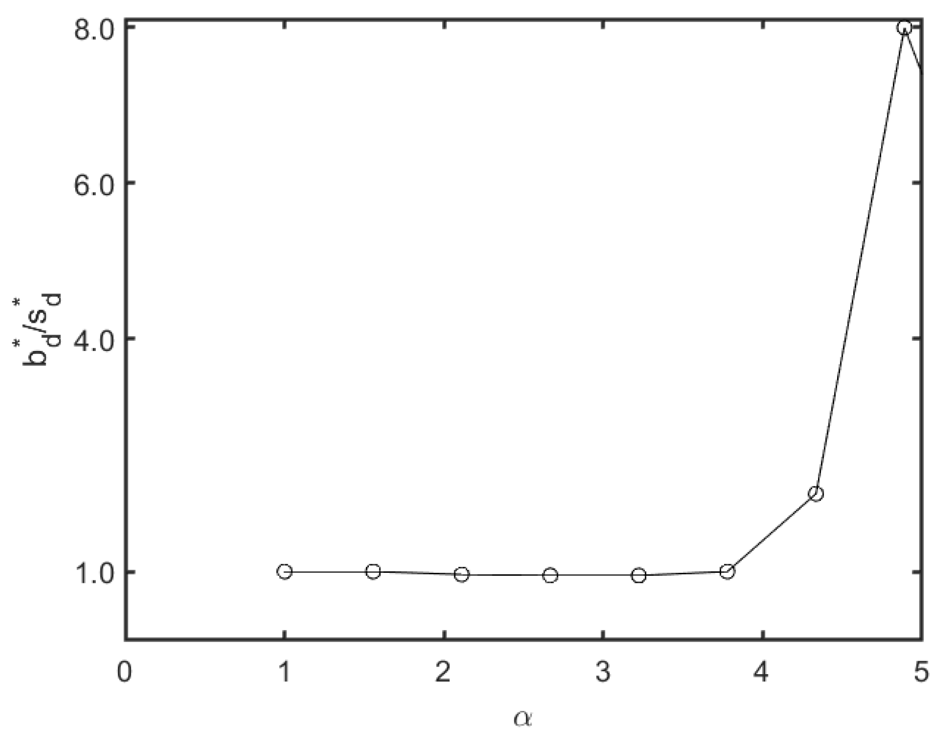
5.2. Impacts of Loading

The analysis impacts of ρ 1 on the V t / V d and z t / z d . We fix ρ 2 = 0.8 , c 1 = 2 , c 2 = 4 , c 3 = 0.4 , c 4 = 0.25 , b = 2 , h d = 1 , h t = 1.5 . For 0 z 0 C d and 0 z 0 C t , we let z 0 = 25 ; for C d < z 0 and C t < z 0 , we let z 0 = 150 .
Figure 3 shows that V t / V d > 1 always holds, and this ratio increases as M increases. This means that under a carbon cap-and-trade environment, DD is still more suitable than pure MTS for mass customization. But V t / V d decreases when the loading of stage-1 increases, which means that the relative advantage of DD becomes more capacity-constrained. The comparison between Figure 3a,b shows that the revenue from emission trading significantly improves the cost function. For example, when ρ 1 = 0.42 and M = 3 , if the manufacturer purchases emission allowances, V t / V d = 2 ; if the manufacturer sells emission allowances, V t / V d = 3.52 . This indicates that the profit generated from carbon trading increases the cost advantage of DD.
As shown in Table 2 and Table 3, with the increase of ρ 1 , the ratio of emissions after the trading decision in the DD system and the pure MTS system, i.e., z t / z d gradually decrease and approach 1. As the number of product types increases, the emission advantage of DD weakens. By comparing Table 2 and Table 3, it can be found that selling emissions allowances can improve the emission advantage of the DD system.
Observation 1.
Under a carbon cap-and-trade system, the DD system has greater cost and emission reduction advantages compared to the pure MTS system. Choosing to sell emission allowances further enhances the advantages of the DD system.
When analyzing the impacts of ρ 2 on the V t / V d and z t / z d , we fix ρ 1 = 0.8 , and ρ 2 becomes variable. Based on Figure 4, the trend of V t / V d is decreasing as ρ 2 increases, meaning that the cost advantage of DD diminishes with the increase of ρ 2 . The DD system still plays a suitable role in mass customization. This is because the only way to reduce stage-2 delays in DD is by holding a more semi-finished product inventory. To meet the target order fulfillment time, DD has to proportionally increase its inventory, directly leading to a gradual decline in its cost advantage.
As shown in Table 4 and Table 5, z t / z d decreases with the increase of ρ 2 , which is opposite to the trend of  z t / z d with ρ 1 . However, the reason is the same as in Figure 4. When ρ 2 = 0.84 and its subsequent values are considered, a sharp decrease in the value of z t / z d . Therefore, to maintain the stability of the production system, it is best to control the value of ρ 2 to be below 0.8.
Comparing with two emission decisions, the systems receive a cost and emission advantage under the purchasing emissions allowances decisions. In the case of more product varieties, although the DD system shows clear cost advantages, its emission reduction advantages weaken.
Observation 2.
While  ρ 1 = 0.8  and  ρ 2 0.6 , 0.7 , the DD system can achieve optimal performance in both cost and emission reduction under the purchase emissions allowance decisions.

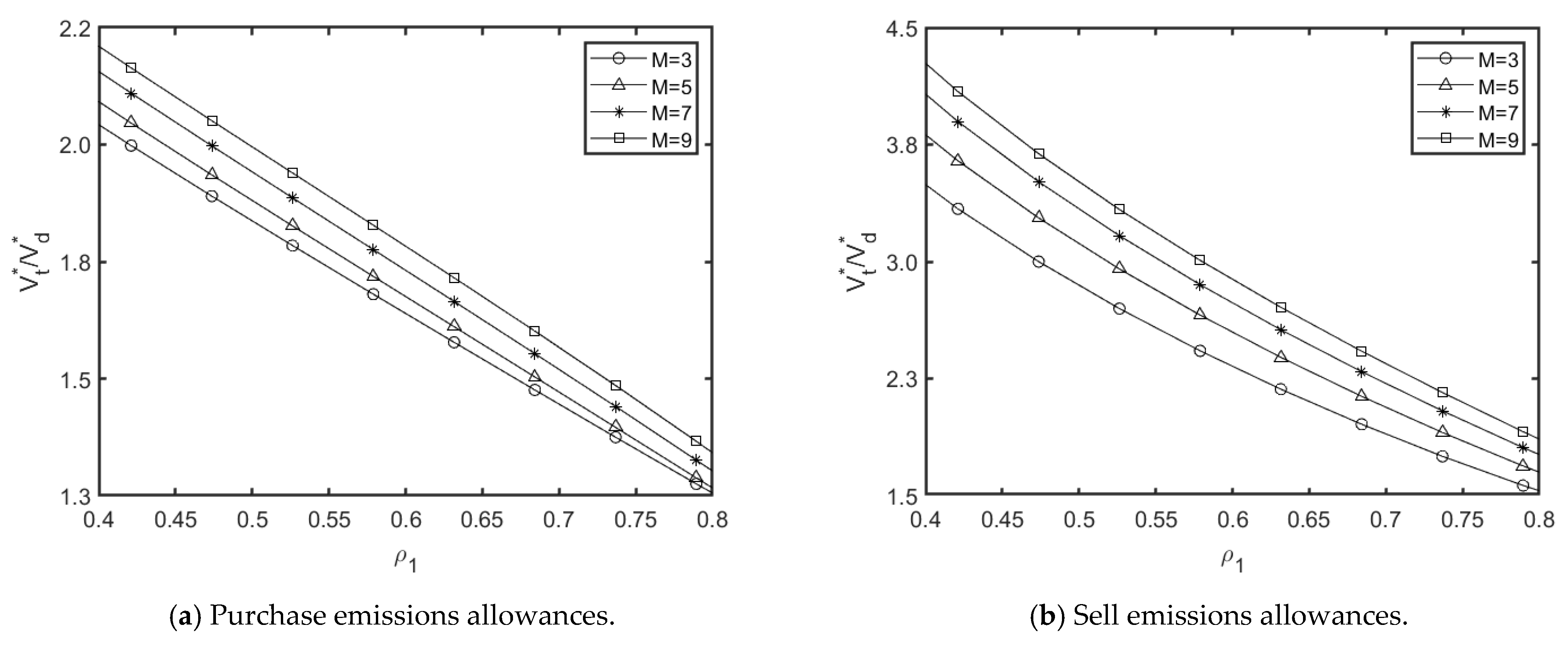
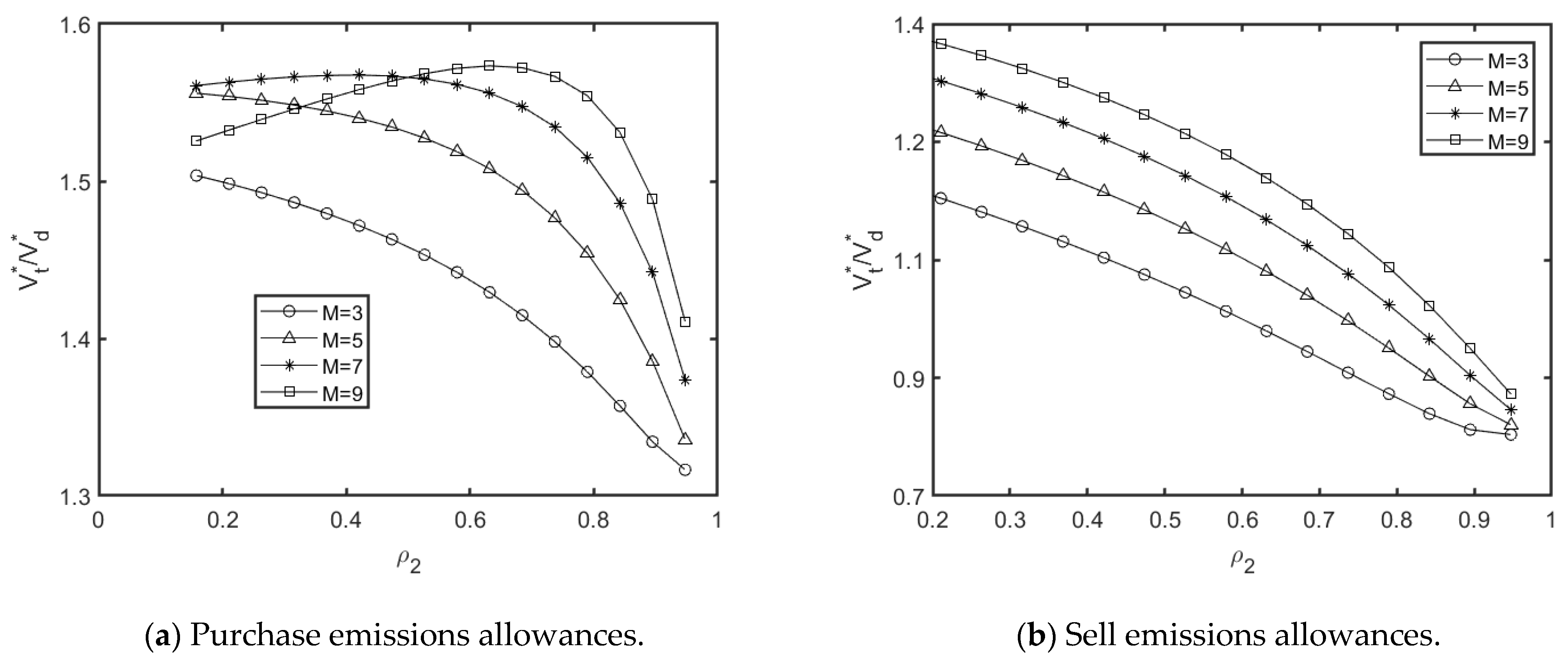
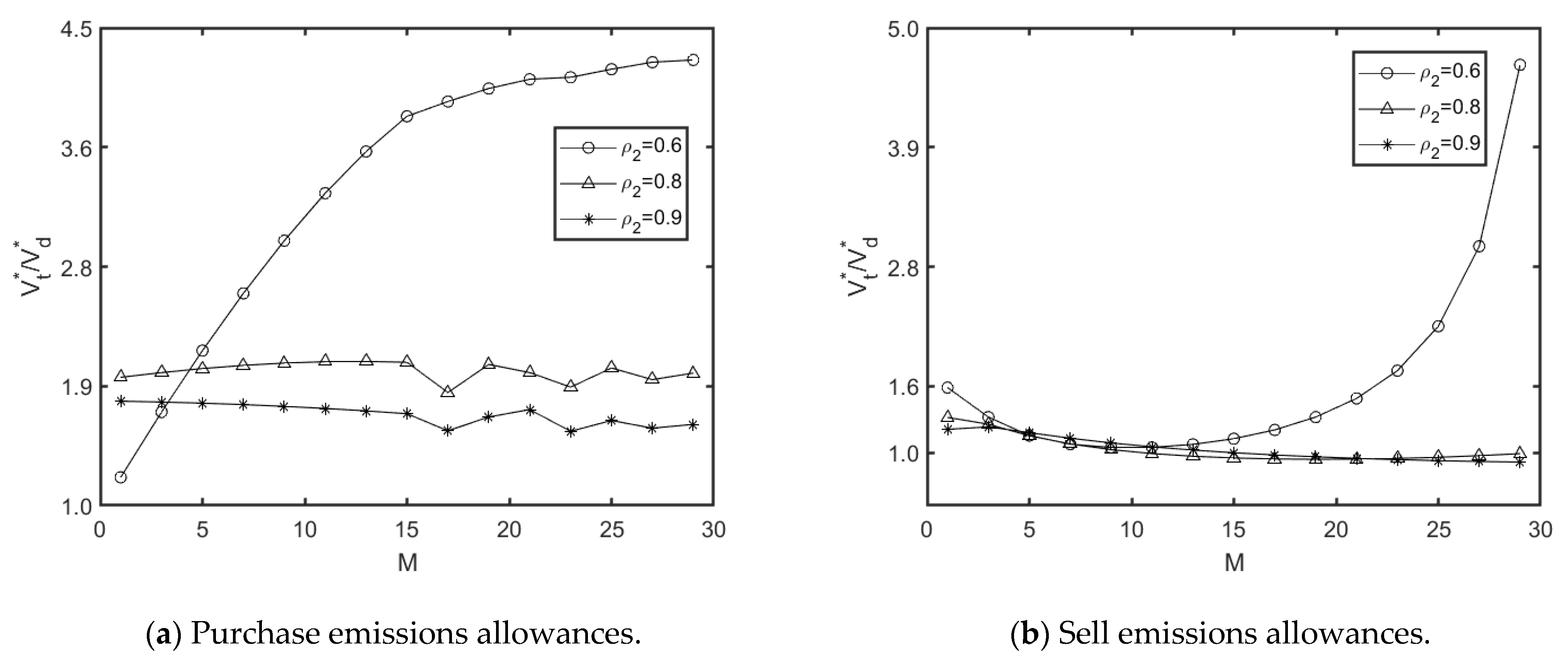
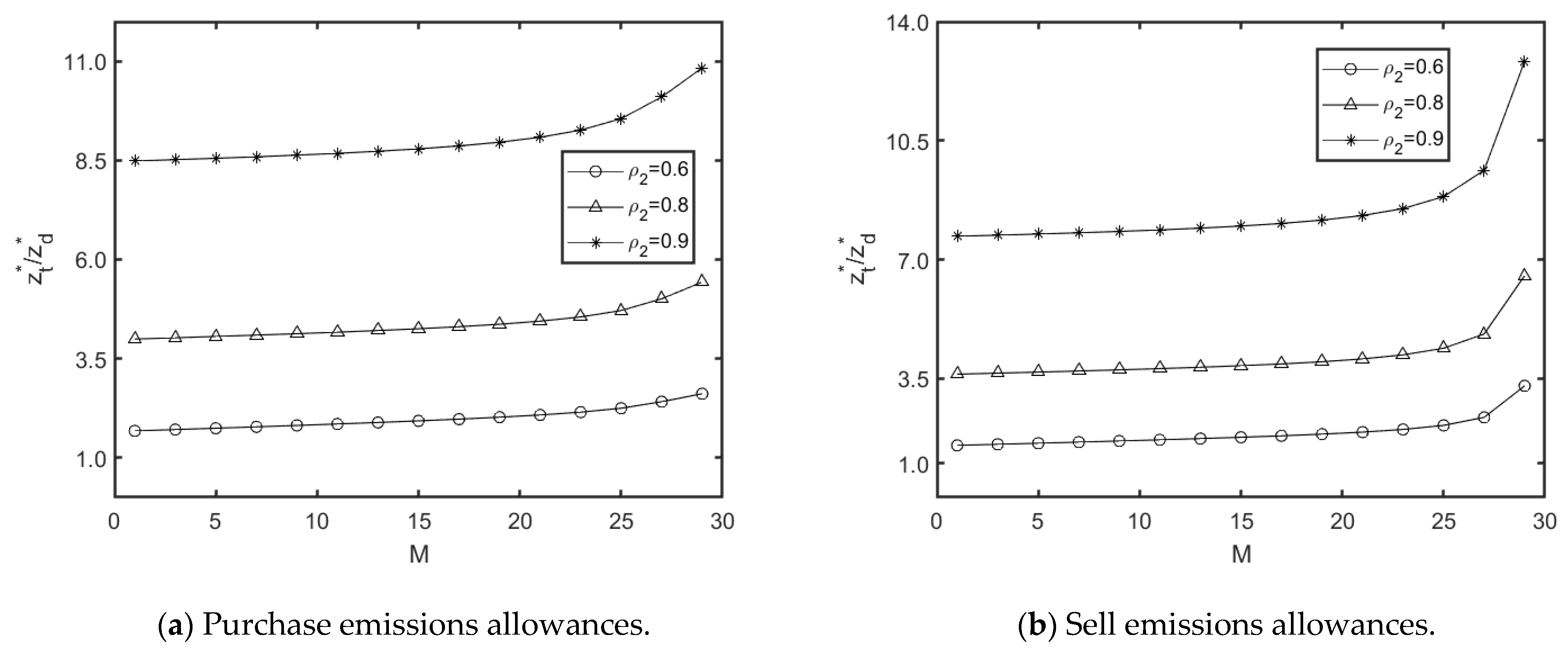
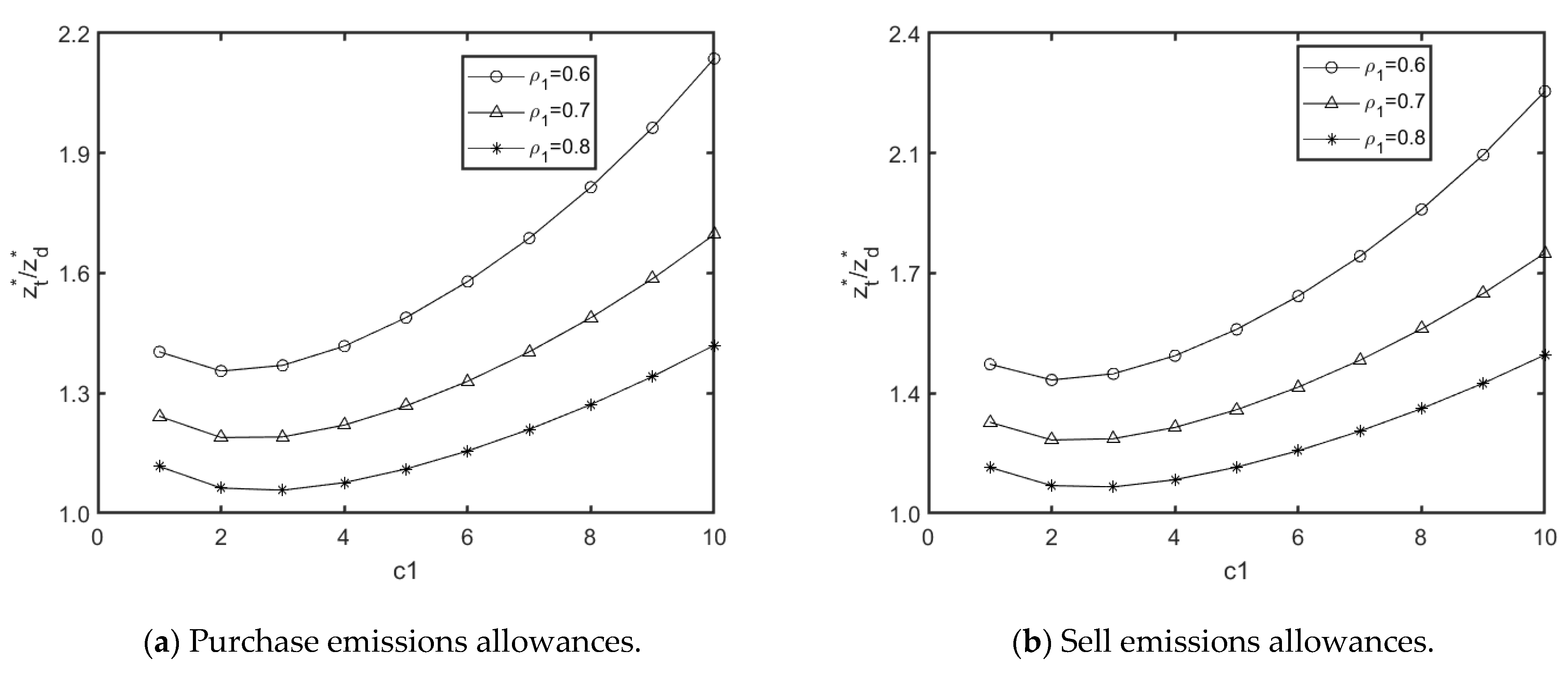
5.3. Sensitivity Study

Next, we study the sensitivity of optimal solutions with the parameters changing.
Figure 5 and Figure 6 show that as the product variety increases, the cost and emission advantages of the DD system increase when ρ 2 = 0.6 ; whereas, while ρ 2 = 0.9 , the cost optimization capability of the DD system weakens. This implies that for stage-2, production capacity can be controlled moderately, and there is no need to blindly expand equipment or increase labor.
As the c1 value increases in Figure 7 and Figure 8, the cost advantage of the DD system decreases, while the emission advantage of the DD system increases. When c1 is relatively large, the cost advantage of the DD system becomes more apparent when the ρ 1 is relatively low. This indicates that when carbon emission control is prioritized, the cost optimization capability of the DD system weakens.

6. Conclusions

This paper primarily investigates the production decision and cost optimization of a multi-product delayed differentiation (DD) system with capacity and order fulfillment time constraints in a carbon trading environment. We model the two-stage production system based on queuing theory and derive the optimal analytical solution for inventory levels and cost function. We found that under carbon policies, the DD system still holds an advantage. Additionally, our research provides three management recommendations.
First, when the order-fulfillment time is relatively flexible, the manager can appropriately reduce the inventory levels of semi-finished goods. Second, production should be primarily focused on stage-1, and the manager needs to allocate more resources to enhance the load capacity of this stage, while stage-2 should maintain a moderate load capacity. Finally, the unit carbon emissions of each production stage are positively correlated to costs, so it may be worth considering the introduction of emission reduction technologies.
This paper researched the study of fixed carbon permit trading prices. A future research direction is to consider time-dependent stochastic carbon trading prices. Other possible extensions include modeling the optimal cost in the context of multiple decision periods.

Author Contributions

Conceptualization, S.X. and L.Y.; methodology, L.Y.; validation, S.X. and L.Y.; formal analysis, S.X. and L.Y.; investigation, S.X. and L.Y.; data curation, S.X. and L.Y.; writing—original draft preparation, L.Y; writing—review and editing, S.X. and L.Y.; visualization, S.X. and L.Y.; Software, L.Y.; supervision, S.X.; project administration, S.X. All authors have read and agreed to the published version of the manuscript.

Funding

This work was supported by Humanities and Social Sciences Youth Foundation, Ministry of Education of the People’s Republic of China, grant number 22YJCZH221; and the Key Project of the Hunan Provincial Department of Education, grant number 23A0254; and the General Project of Hunan Provincial Water Resources Department, grant number XSKJ2023059-39; Hunan Provincial Graduate Research and Innovation Project, grant number CX20230926; The General Project of the Fifth National Economic Census in Hunan Province, Grant number hnwjp14.

Institutional Review Board Statement

Not applicable.

Informed Consent Statement

Not applicable.

Data Availability Statement

The data presented in this study are available upon request to the corresponding author.

Conflicts of Interest

The authors declare no conflicts of interest.

Appendix A

The carbon trading situation can be divided into two types: (1) if z t > z 0 , then purchase emission allowances; (2) if z t < z 0 , then sell emission allowances.
(1)
if z t > z 0 ,
  • C t z t > z 0 ,
    V t = μ ( z t z 0 ) + h t I t ( s t ) + b B ¯ t ( s t ) + π C t z t ;
  • z t C t > z 0 ,
    V t = μ ( z t z 0 ) + h t I t ( s t ) + b B ¯ t ( s t ) ;
  • z t > z 0 > C t ,
    V t = μ ( z t z 0 ) + h t I t ( s t ) + b B ¯ t ( s t ) .
In the case of purchasing emission allowances, the optimal cost is  V t = μ ( z t z 0 ) + h t I t ( s t ) + b B ¯ t ( s t ) ; therefore, z t C t , μ ( z t z 0 ) should be as small as possible to further optimize the cost. Since z 0 is a predetermined exogenous variable, the smaller z t promotes the more optimal cost, i.e., the optimal value of z t is C t .
(2)
if z t < z 0 ,
  • C t > z 0 > z t ,
    V t = ν ( z 0 z t ) + h t I t ( s t ) + b B ¯ t ( s t ) + π C t z t ;
  • z 0 > C t z t ,
    V t = ν ( z 0 z t ) + h t I t ( s t ) + b B ¯ t ( s t ) + π C t z t ;
  • z 0 > z t C t
    V t = ν ( z 0 z t ) + h t I t ( s t ) + b B ¯ t ( s t ) ;
In the case of selling emission allowances, the optimal cost is V t = ν ( z 0 z t ) + h t I t ( s t ) + b B ¯ t ( s t ) ; therefore, z t C t , v ( z 0 z t ) should be as small as possible to further optimize the cost, Similarly, the optimal value of z t is C t .
In summary, whether purchasing or selling emission allowances, to ensure the cost function is minimized, the prerequisite is z t * = C t .

Appendix B

The solution sequence for the optimal solution is as follows: z t V t s t .
If z t z 0 , in Equation (12) [ ( z t z 0 ) ] + = 0 , substituting z t = C t into Equation (12) yields: V t = μ ( C t z 0 ) + h t I ¯ t ( s t ) + b B ¯ t ( s t ) , where is an expression with respect to the decision variable s t . Therefore, the optimal solution is obtained by solving the gradient equation. However, solving it in MATLAB R2022a shows that there is no explicit solution. We provide an explanation for one case, while the other case follows similarly.

Appendix C

Since demand is Poisson and we approximate the inter-arrival times of units at stage-2 to follow an exponential distribution, we assume stage-2 as the M/M/1 queue, given r jobs in the system. Therefore, at any given observation moment, we obtain the probability p d ( k j ) of type k j products as:
p d ( k j ) = ( 1 ρ 1 ) ρ 1 r .
To reduce the complexity of the calculations, we assume D j max ; therefore:
k j = 0 D j max k j p d ( k j ) = ρ 1 1 ρ 1
(1)
if z d z 0 ,
V d * = μ ( z d z d 0 ) + h d I ¯ d ( s d ) + b B ¯ d ( s d ) = μ ( ( c 1 + c 2 ) k j = 0 D j max k j p d ( k j ) + c 1 s d + c 4 I ¯ d ( s d ) z d 0 ) + h d I ¯ d ( s d ) + b B ¯ d ( s d ) = μ ( ( c 1 + c 2 ) ρ 1 1 ρ 1 + c 1 s d + c 4 s d ( ρ 1 ( 1 ρ 1 s d ) 1 ρ 1 ) z d 0 ) + h d s d ( ρ 1 ( 1 ρ 1 s d ) 1 ρ 1 ) + b ρ 2 1 ρ 2 + ρ 1 s d + 1 1 ρ 1
(2)
if z d < z 0 ,
V d * = v ( z d 0 z d ) + h d I ¯ d ( s d ) + b B ¯ d ( s d ) = v ( ( c 1 + c 2 ) k j = 0 D j max k j p d ( k j ) + c 1 s d + c 4 I ¯ d ( s d ) z d 0 ) + h d I ¯ d ( s d ) + b B ¯ d ( s d ) = v ( ( c 1 + c 2 ) ρ 1 1 ρ 1 + c 1 s d + c 4 s d ( ρ 1 ( 1 ρ 1 s d ) 1 ρ 1 ) z d 0 ) + h d s d ( ρ 1 ( 1 ρ 1 s d ) 1 ρ 1 ) + b ρ 2 1 ρ 2 + ρ 1 s d + 1 1 ρ 1

Appendix D

If z d z 0 , let
V d * s d = μ ( ( c 1 + c 2 ) ρ 1 1 ρ 1 + c 1 s d + c 4 s d ( ρ 1 ( 1 ρ 1 s d ) 1 ρ 1 ) z d 0 ) + h d s d ( ρ 1 ( 1 ρ 1 s d ) 1 ρ 1 ) + b ρ 2 1 ρ 2 + ρ 1 s d + 1 1 ρ 1 / s d = 0
Theorem 5 can be obtained by solving it in MATLAB R2022a.

References

  1. European Environment Agency. EU Emissions Trading System (ETS) Data Viewer. Available online: https://www.eea.europa.eu/data-and-maps/dashboards/emissions-trading-viewer-1/ (accessed on 10 May 2024).
  2. Shao, X.F.; Dong, M. Comparison of order-fulfilment performance in MTO and MTS systems with an inventory cost budget constraint. Int. J. Prod. Res. 2012, 50, 1917–1931. [Google Scholar] [CrossRef]
  3. Rafiei, H.; Rabbani, M.; Alimardani, M. Novel bi-level hierarchical production planning in hybrid MTS/MTO production contexts. Int. J. Prod. Res. 2013, 51, 1331–1346. [Google Scholar] [CrossRef]
  4. Ebadian, M.; Rabbani, M.; Jolai, F.; Torabi, S.; Tavakkoli-Moghaddam, R. A new decision-making structure for the order entry stage in make-to-order environments. Int. J. Prod. Econ. 2008, 111, 351–367. [Google Scholar] [CrossRef]
  5. Van Donk, D.P. Make to stock or make to order: The decoupling point in the food processing industries. Int. J. Prod. Econ. 2001, 69, 297–306. [Google Scholar] [CrossRef]
  6. Olhager, J. Strategic positioning of the order penetration point. Int. J. Prod. Econ. 2003, 319–329. [Google Scholar] [CrossRef]
  7. Adan, I.J.B.F.; van der Wal, J. Combining make to order and make to stock. OR Spectr. 1998, 20, 73–81. [Google Scholar] [CrossRef]
  8. Eivazy, H.; Rabbani, M.; Ebadian, M. A developed production control and scheduling model in the semiconductor manufacturing systems with hybrid make-to-stock/make-to-order products. Int. J. Adv. Manuf. Technol. 2009, 45, 968–986. [Google Scholar] [CrossRef]
  9. Sun, X.; Ji, P.; Sun, L.; Wang, Y. Positioning multiple decoupling points in a supply network. Int. J. Prod. Econ. 2008, 113, 943–956. [Google Scholar] [CrossRef]
  10. Lee, H.L.; Billington, C. Designing products and processes for postponement. In Management of Design: Engineering and Management Perspectives; Springer: Berlin/Heidelberg, Germany, 1994; pp. 105–122. [Google Scholar]
  11. Lee, H.L.; Tang, C.S. Modeling the costs and benefits of delayed product differentiation. Manag. Sci. 1997, 43, 40–53. [Google Scholar] [CrossRef]
  12. Swaminathan, J.M.; Tayur, S.R. Managing broader product lines through delayed differentiation using vanilla boxes. Manag. Sci. 1998, 44, 161–172. [Google Scholar] [CrossRef]
  13. Gupta, D.; Benjaafar, S. Make-to-order, make-to-stock, or delay product differentiation? A common framework for modeling and analysis. IIE Trans. 2004, 36, 529–546. [Google Scholar] [CrossRef]
  14. Jewkes, E.M.; Alfa, A.S. A queueing model of delayed product differentiation. Eur. J. Oper. Res. 2009, 199, 734–743. [Google Scholar] [CrossRef]
  15. Almehdawe, E.; Jewkes, E. Performance analysis and optimization of hybrid manufacturing systems under a batch ordering policy. Int. J. Prod. Econ. 2013, 144, 200–208. [Google Scholar] [CrossRef]
  16. Su, J.C.P.; Chang, Y.-L.; Ferguson, M.; Ho, J.C. The impact of delayed differentiation in make-to-order environments. Int. J. Prod. Res. 2010, 48, 5809–5829. [Google Scholar] [CrossRef]
  17. Zhou, W.H.; Huang, W.X.; Zhang, R.Q. A two-stage queueing network on form postponement supply chain with correlated demands. Appl. Math. Model. 2014, 38, 2734–2743. [Google Scholar] [CrossRef]
  18. Fei, Q.; Kong, N.; Zhao, L. Investment decision optimization for delayed product differentiation based on queuing theory. J. Southeast Univ. (Engl. Ed.) 2018, 34, 532–539. [Google Scholar]
  19. Bandaly, D.C.; Hassan, H.F. Postponement implementation in integrated production and inventory plan under deterioration effects: A case study of a juice producer with limited storage capacity. Prod. Plan. Control. 2019, 31, 322–337. [Google Scholar] [CrossRef]
  20. Zhang, B.; Xu, L. Multi-item production planning with carbon cap and trade mechanism. Int. J. Prod. Econ. 2013, 144, 118–127. [Google Scholar] [CrossRef]
  21. Cao, K.Y.; Xu, X.P.; Wu, Q.; Zhang, Q.P. Optimal production and carbon emission reduction level under cap-and-trade and low carbon subsidy policies. J. Clean. Prod. 2017, 167, 505–513. [Google Scholar]
  22. Hu, B.Y.; Feng, Y. Emission reduction decision and coordination of a make-to-order supply chain with two products under cap-and-trade regulation. Comput. Ind. Eng. 2018, 119, 131–145. [Google Scholar]
  23. Ping, H.; Zhang, W.; Xu, X.; Bian, Y. Production lot-sizing and carbon emissions under cap-and-trade and carbon tax regulations. J. Clean. Prod. 2015, 103, 241–248. [Google Scholar]
  24. Xu, X.; Zhang, W.; He, P.; Xu, X. Production and pricing problems in make-to-order supply chain with cap-and-trade regulation. Omega Int. J. Manag. Sci. 2017, 66, 248–257. [Google Scholar] [CrossRef]
  25. Xiong, S.Y.; Feng, Y.Y.; Huang, K. Optimal MTS and MTO Hybrid Production System for a Single Product Under the Cap-And-Trade Environment. Sustainability 2020, 12, 24–26. [Google Scholar] [CrossRef]
  26. Gong, X.; Zhou, S.X. Optimal production planning with emissions trading. Oper. Res. 2013, 61, 908–924. [Google Scholar] [CrossRef]
  27. Yuan, B.Y.; Gu, B.M.; Xu, C.M. The Multi-Period Dynamic Optimization with Carbon Emissions Reduction under Cap-and-Trade. Discret. Dyn. Nat. Soc. 2019, 1, 1–12. [Google Scholar] [CrossRef]
  28. Williams, T.M. Special products and uncertainty in production/inventory systems. Eur. J. Oper. Res. 1984, 15, 46–54. [Google Scholar] [CrossRef]
  29. Carr, S.; Duenyas, I. Optimal Admission Control and Sequencing in a Make-To-Stock/Make-To-Order Production System. Oper. Res. 2000, 48, 709–720. [Google Scholar] [CrossRef]
  30. Gupta, D.; Weerawat, W. Supplier–manufacturer coordination in capacitated two-stage supply chains. Eur. J. Oper. Res. 2006, 175, 67–89. [Google Scholar] [CrossRef]
Figure 1. The two systems under consideration: (a) pure MTS system; (b) system with DD.
Systems 13 00161 g001
Figure 2. Optimal Inventory Comparison: DD with Emissions Trade Vs. DD without.
Systems 13 00161 g002
Figure 3. Impact of stage-1 loading on the cost advantage of DD.
Systems 13 00161 g003
Figure 4. Impact of stage-2 loading on the cost advantage of DD.
Systems 13 00161 g004
Figure 5. Impact of the quantity of products on the cost advantage of DD.
Systems 13 00161 g005
Figure 6. Impact of the quantity of products on the emissions advantage of DD.
Systems 13 00161 g006
Figure 7. Impact of the unit emissions of stage-1 on the cost advantage of DD.
Systems 13 00161 g007
Figure 8. Impact of the unit emissions of stage-1 on the emissions advantage of DD.
Systems 13 00161 g008
Table 1. A brief summary of related literature.
PaperSubjects AddressedDemand Product Process StructurePerformance CriteriaSolution Approach
Willams (1984) [28]MTO/MTS
partitioning
Stochastic demand, multi-product, multi-machinesMinimizing sum of inventory holding costs, stock-out, and set-up
costs
Approximations of M/G/m queues
Carr
(2000) [29]
Joint admission control and sequencing problemSingle machine and two types of product
No backordering, no set-up times,
Profit maximizationMarkov decision process for two-class M/M/1
queue
Gupta and
Benjaafar (2004) [13]
inventory management for the semi-finished goods between the two stagesmulti-product,
No set-up cost
Minimizing sum of
inventory holding costs, backorder costs
Approximations of M/M/1 queues
Jewkes and
Alfa (2009) [14]
the optimal point of differentiationa-product, multi-periodsMinimizing sum of costs of order fulfillment delay, costs of holding semi-finished goods in inventory, cost of salvaging.Markov decision process for queue theory
Swaminathan and
Tayur (1998) [12]
the optimal configuration for semi-finished products from the point of view of commonality among different final productssingle-periods and multi-periodsMinimizing sum of stock-out cost, holding costgradient derivative methods for two-stage integer program with recourse
Gupta and Weerawat (2006) [30]looks into coordination between the two stagesdecentralized model: the fixed-markup contract, the simple revenue-sharing contractProfit maximizationApproximations of M/M/1 queues
Table 2. The impact of stage-1 loading on the ratio of z t * / z d * , while the company decides to purchase emissions allowances.
ρ 1 M = 3 M = 5 M = 7 M = 9
0.42 10.54 9.96 9.62 9.40
0.47 8.24 7.77 7.51 7.33
0.53 6.65 6.27 6.05 5.91
0.58 5.49 5.16 4.99 4.87
0.63 4.59 4.31 4.17 4.07
0.68 3.88 3.64 3.51 3.43
0.74 3.30 3.09 2.98 2.92
0.79 2.81 2.63 2.54 2.48
Table 3. The impact of stage-1 loading on the ratio of z t * / z d * , while the company decides to sell emissions allowances.
ρ 1 M = 3 M = 5 M = 7 M = 9
0.42 12.78 11.70 11.18 10.86
0.47 9.73 8.90 8.51 8.26
0.53 7.73 7.07 6.75 6.56
0.58 6.31 5.77 5.51 5.35
0.63 5.25 4.79 4.58 4.45
0.68 4.42 4.03 3.85 3.74
0.74 3.75 3.42 3.27 3.17
0.79 3.20 2.92 2.79 2.71
Table 4. The impact of stage-2 loading on the ratio of z t * / z d * , while the company decides to purchase emissions allowances.
ρ 2 M = 3 M = 5 M = 7 M = 9
0.16 0.99 0.93 0.89 0.87
0.21 1.02 0.96 0.92 0.90
0.26 1.06 0.99 0.95 0.93
0.32 1.10 1.03 0.99 0.97
0.37 1.15 1.08 1.04 1.02
0.42 1.22 1.14 1.10 1.08
0.47 1.30 1.22 1.18 1.15
0.53 1.41 1.32 1.28 1.25
0.58 1.56 1.46 1.42 1.39
0.63 1.79 1.68 1.63 1.60
0.68 2.17 2.03 1.97 1.94
0.74 2.91 2.73 2.66 2.62
0.79 5.10 4.81 4.70 4.64
0.84 0.99 0.93 0.89 0.87
0.89 1.02 0.96 0.92 0.90
0.95 1.06 0.99 0.95 0.93
Table 5. The impact of stage-2 loading on the ratio of z t * / z d * , while the company decides to sell emissions allowances.
ρ 2 M = 3 M = 5 M = 7 M = 9
0.16 0.96 0.88 0.84 0.82
0.21 0.99 0.90 0.86 0.84
0.26 1.01 0.92 0.88 0.86
0.32 1.04 0.95 0.91 0.88
0.37 1.07 0.98 0.93 0.91
0.42 1.11 1.01 0.97 0.94
0.47 1.15 1.05 1.01 0.98
0.53 1.21 1.10 1.05 1.02
0.58 1.28 1.16 1.11 1.08
0.63 1.36 1.24 1.19 1.15
0.68 1.48 1.35 1.29 1.25
0.74 1.63 1.49 1.42 1.38
0.79 1.87 1.70 1.63 1.58
0.84 2.25 2.06 1.97 1.92
0.89 3.01 2.75 2.64 2.57
0.95 5.26 4.83 4.63 4.53
Disclaimer/Publisher’s Note: The statements, opinions and data contained in all publications are solely those of the individual author(s) and contributor(s) and not of MDPI and/or the editor(s). MDPI and/or the editor(s) disclaim responsibility for any injury to people or property resulting from any ideas, methods, instructions or products referred to in the content.

