1. Introduction
While driving robust economic growth, the manufacturing sector, as a cornerstone of the national economy, faces significant challenges related to resource consumption and environmental pollution. In response to the growing concerns over global climate change and energy scarcity, low-carbon manufacturing has emerged as a pivotal strategy for achieving sustainable development within the industry. Against this backdrop, with the increasing adoption of low-carbon manufacturing principles, the flexible job-shop scheduling problem, a central issue in manufacturing production management, has expanded its optimization focus from traditional production efficiency to encompass multi-dimensional objectives such as production efficiency, energy consumption, and carbon emissions reduction. An increasing number of researchers are now concentrating their efforts on low-carbon scheduling optimization in flexible job shops, aiming to develop innovative strategies that effectively minimize energy consumption and carbon emissions while ensuring sustained production efficiency.
In the domain of low-carbon scheduling models, Dai et al. [
1] proposed a multi-objective optimization framework for energy-efficient flexible job shop scheduling, which integrates transportation constraints. The primary objectives were to minimize both total energy consumption and makespan. To address this complex problem, they employed an advanced genetic algorithm that combines particle swarm optimization and simulated annealing techniques. Tian et al. [
2] investigated the dynamic energy-efficient scheduling challenge in a flexible job shop characterized by a multi-product, small-batch production environment. They formulated a multi-objective optimization model that considers total energy consumption, makespan, and processing costs. A dual-population differential artificial bee colony algorithm was introduced as an effective approach to optimize resource allocation in aerospace manufacturing. Chen et al. [
3] further expanded on this research by accounting for shop heterogeneity and the influence of job insertion and transfer on scheduling decisions. They developed a mathematical model aimed at minimizing total weighted tardiness and total energy consumption, leveraging a deep reinforcement learning framework to derive optimal scheduling strategies in dynamic settings.
In addition to energy consumption, some researchers utilize carbon emissions and noise levels as indicators to assess the environmental impact of production processes. Piroozfard et al. [
4] integrated classical and environment-oriented objective functions in scheduling problems to formulate a multi-objective flexible job shop scheduling problem aimed at simultaneously minimizing total carbon footprint and total late work. Sun et al. [
5] proposed a mathematical model for the multi-objective flexible job shop scheduling problem (MO-FJSP), which considers minimum completion time, carbon emissions and machine loads, thereby addressing environmental impacts while maintaining production efficiency. Shun et al. [
6] presented an energy cost model based on time-of-use electricity pricing, constructing a multi-objective optimization framework to simultaneously minimize costs, reduce carbon emissions, and enhance customer satisfaction. This model was solved using an enhanced genetic algorithm. Wang et al. [
7] extended the objective system for low-carbon scheduling in flexible job shops by developing a comprehensive scheduling optimization model that integrates makespan, total tardiness, bottleneck machine processing load, and total system carbon emissions across four dimensions. Their enhanced multi-objective evolutionary algorithm (MOEA) significantly improved solution efficiency. Yu et al. [
8] introduced a bi-objective optimization model for distributed flexible job shop scheduling scenarios, focusing on minimizing makespan and total energy consumption. Xu et al. [
9] expanded the scope of the distributed flexible job shop scheduling problem by incorporating workpiece job outsourcing and proposed a multi-objective mathematical model. This model integrates key performance indicators such as makespan, cost, quality and carbon emissions, thereby meeting the practical needs of modern manufacturing enterprises. Li et al. [
10] addressed the multi-objective green flexible job shop scheduling problem (MGFJSP) by considering carbon emissions, noises and wastes to comprehensively assess the degree of environmental pollution. They established an MGFJSP model with the optimization goals of minimizing the makespan and the degree of environmental pollution. Zhao et al. [
11] investigated the multi-objective green flexible job shop scheduling problem (MGFJSP) by considering factors such as carbon emissions, noise levels, and waste generation to comprehensively evaluate environmental pollution. They formulated an MGFJSP model with dual optimization objectives: minimizing both the makespan and the degree of environmental pollution.
Several representative methods have been proposed by both domestic and international scholars in the field of multi-objective optimization algorithms. For instance, Deb et al. [
12] introduced the NSGA-II algorithm, Zitzle et al. [
13] developed the SPEA algorithm, and Knowles et al. [
14] proposed the PESA algorithm. Among these, NSGA-II has gained widespread adoption, prompting many researchers to enhance its solution efficiency and accuracy through various improvements. Gong et al. [
15], for example, devised a three-layer coding structure to represent process selection, equipment allocation, and personnel scheduling, enabling dynamic configuration of equipment and personnel within a flexible manufacturing environment. They utilized a hybrid genetic algorithm for multi-objective green scheduling. Ning et al. [
16] proposed an enhanced quantum genetic algorithm utilizing double-chain coding to address the challenge of machining route selection in shop floor scheduling. Jiang et al. [
17] incorporated Tent chaotic mapping into the NSGA-II algorithm to refine its coding mechanism and developed an improved elite retention strategy based on an external archive set to enhance the algorithm’s overall performance. Liu et al. [
18] designed a hybrid algorithm that integrates genetic algorithms, firefly optimization, and green transportation strategies to address the dual-objective optimization problem of minimizing energy consumption and reducing completion time. Chen et al. [
19] proposed an enhanced Q-learning-based non-dominated sorting genetic algorithm (QNSGA-II) to solve the dynamic flexible job shop scheduling problem while considering limited transportation resources. Wang et al. [
20] combined a genetic algorithm with a differential evolution algorithm to address the energy-saving scheduling challenge in flexible job shops, incorporating equipment maintenance and logistics transportation.
Beyond the NSGA-II algorithm, researchers have delved into additional intelligent optimization algorithms and their hybrid variants. Liu et al. [
21] investigated the performance of the fruit fly optimization algorithm (FOA) in addressing multi-objective scheduling optimization problems and developed a hybrid fruit fly optimization algorithm (HFOA) to effectively solve these problems. Lu et al. [
22] introduced a bi-population based discrete bat algorithm (BDBA), which was specifically designed considering the characteristics of job shop scheduling problems, aiming to minimize the combined cost of energy consumption and completion time. Jian et al. [
23] proposed an enhanced multi-objective wolf pack algorithm (MOWPA) that incorporates genetic algorithm principles, effectively addressing complex scheduling models by optimizing both makespan and total energy consumption. Zhou et al. [
24] introduced an improved grey wolf optimization algorithm for bi-objective optimization of carbon emissions and manufacturing costs in flexible job shop scheduling, providing a groundbreaking approach to scheduling challenges within the framework of green manufacturing. Li et al. [
25] devised an advanced artificial bee colony algorithm based on three-dimensional vector encoding and dynamic neighborhood search strategies, aiming to minimize completion time while mitigating environmental impact in flexible job shop scheduling problems. Gu et al. [
26] enhanced the artificial bee colony algorithm by integrating a two-tier population initialization method, an improved crossover and neighborhood search strategy, a greedy selection mechanism and a scout bee approach to ensure global convergence. This integrated framework was specifically designed to address the multi-objective low-carbon flexible job shop scheduling problem. Luan et al. [
27] and Jiang et al. [
28] independently developed discrete whale optimization algorithms and modified African buffalo optimization algorithms, two innovative bio-inspired metaheuristic methods, to tackle low-carbon flexible job shop scheduling problems.
Based on the aforementioned research, the following summary can be drawn: (1) Studies on low-carbon flexible job shop scheduling problem predominantly emphasize traditional optimization objectives, such as makespan minimization, total machine energy consumption, workload balancing, and energy cost reduction. Nevertheless, the quantitative evaluation of direct carbon emissions has received relatively limited attention. (2) Regarding algorithm application, the NSGA-II algorithm has emerged as a prevalent choice for its robust multi-objective optimization capabilities. However, its susceptibility to premature convergence often leads to suboptimal solutions in complex scheduling scenarios, thereby constraining its effectiveness in addressing intricate scheduling challenges. Further research is warranted to investigate alternative intelligent optimization algorithms.
Prior studies largely optimize processing-related emissions, whereas transport and auxiliary loads are often simplified or omitted. This study explicitly integrates these sources into a unified tri-objective framework and tailor INDBO (GLR + IPOX–UX + non-dominated sorting) for the resulting multi-objective trade-offs, situating the contribution alongside recent benchmark practices.
Companies should not only strive to achieve optimal levels of economic efficiency but also ensure adequate levels of environmental and social efficiency [
29]. Thus, this paper aims to conduct a comprehensive evaluation of the environmental impact associated with workpiece machining. It enhances the diversity and comprehensiveness of optimization objectives, with particular emphasis on flexible job shops that manufacture traditional mechanical components. By adopting an integrated perspective of the component manufacturing process, the proposed model incorporates both machining and transportation phases. The optimization objectives focus on minimizing the maximum completion time, total carbon emissions, and production costs, thereby establishing a low-carbon scheduling framework for flexible job shops. In terms of algorithm design, the model is solved using an INDBO algorithm. Compared to existing studies, the application of this INDBO algorithm to job shop scheduling problems remains relatively unexplored, highlighting significant potential for innovation. Finally, instance simulations and comparative experiments conducted in a traditional mechanical machining workshop demonstrate the feasibility and superiority of the proposed model and algorithm, providing valuable decision-support tools for the low-carbon transformation of the manufacturing industry.
2. Problem Description
The low-carbon scheduling problem in a flexible job shop for manufacturing mechanical components can be formulated as follows: Given a fixed layout of a mechanical production workshop with predefined machine locations, a set of n jobs is considered to be processed, denoted by N = {N
1, N
2, …, N
i, …, N
n}. There exists a set of m processing machines, represented by M = {M
1, M
2, …, M
j, …, M
m}. Each job N
i comprises k
i operations, each operation being denoted by O
io (where o = 1, 2, …, k
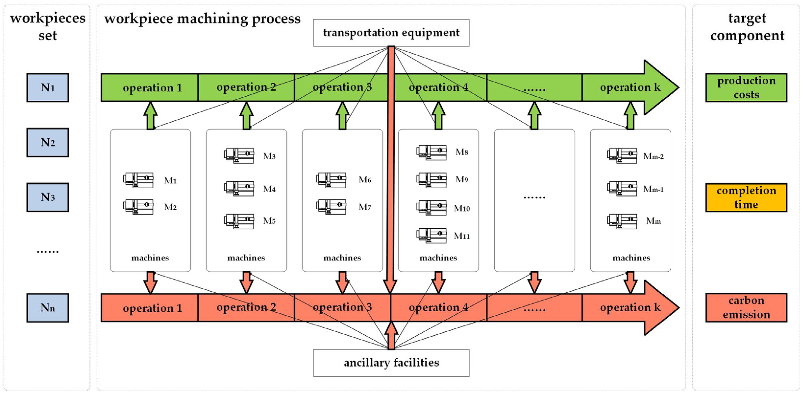
i), and the processing sequence of operations for each job is predetermined. For each operation, there is a selection of parallel machines with identical functionality but varying processing efficiencies, resulting in different processing times for each machine option. The objective of the scheduling optimization is to select the most suitable machines for each operation of every job, determine the start times for each machine, and establish the processing sequence of operations on each machine. This aims to minimize carbon emissions during job processing in the workshop while ensuring production efficiency and controlling production costs. The detailed process is illustrated in
Figure 1.
In this study, case-specific assumptions—including continuous operation, time-zero availability of jobs and the absence of failures or batch variations—are adopted, as the case reflects planned production runs in which maintenance activities and changeovers are scheduled outside the planning horizon, demand is stable, and equipment reliability remains high throughout the evaluation period. These scope conditions facilitate a focused analysis of the key trade-offs among makespan, emissions and cost; their broader applicability is discussed in
Section 3.
Raw material consumption is considered a constant in the calculations, as it remains invariant with respect to process flow adjustments. The carbon emissions and production costs associated with CNC equipment energy consumption, transportation equipment energy consumption, auxiliary facility energy consumption, tool wear, and cutting fluid usage are intricately tied to production scheduling decisions. Subsequent waste material processing is generally performed independently, and its corresponding carbon emissions exhibit minimal sensitivity to the shop scheduling scheme; hence, they are excluded from consideration in the low-carbon scheduling optimization problem.
To facilitate the analysis of the problem, the following assumptions are made:
(1) Equipment failures and material shortages are disregarded in this study.
(2) The workshop infrastructure is assumed to remain fully operational throughout the entire process, from the initiation of processing the first workpiece to the completion of the last, without any interruptions.
(3) The machine tools within the workshop are assumed to operate continuously from the start of processing the first workpiece to the conclusion of processing the last, with no shutdowns.
(4) Variations in batch production for different workpieces are not taken into account.
(5) The influence of workers on production is excluded from consideration.
Additionally, the following constraints must be satisfied during workpiece processing:
(1) A single operation of the same workpiece can only be executed by one machine at a time.
(2) One machine can only handle one operation of a workpiece at a time.
(3) All operations of the same workpiece are subject to precedence constraints, including transportation time between adjacent operations; there are no precedence constraints between operations of different workpieces.
(4) The priorities of different workpieces are equal, and the priorities of machines capable of performing the same operation are also equal.
(5) Once processing begins, each operation of every workpiece cannot be interrupted.
(6) All workpieces and equipment are available from the initial time (time zero).
Based on the problem description, the relevant parameters and variables have been formally defined as shown in
Table 1.
3. Model Construction
This study focuses on the core trade-offs under standard simplifying assumptions, including the absence of machine failures or worker-related effects, continuous operation without interruptions, fixed batch sizes and full availability of jobs and machines at time zero. These assumptions align with the characteristics of this case setting and facilitate tractable optimization; however, they may restrict the direct applicability of the results in environments characterized by frequent operational disruptions or flexible batching policies.
This paper provides a comprehensive synthesis of the machining process for mechanical components in a job shop environment. It elaborates on the selection of optimization objectives by employing machining time as an efficiency metric, production cost as an economic indicator, and carbon emissions as an environmental measure. The aim is to construct a multi-objective flexible job shop low-carbon scheduling mathematical model, with the objectives of minimizing the maximum completion time, total carbon emissions, and production costs.
- (1)
Maximum completion time
The maximum completion time, also known as makespan, serves as a critical metric for evaluating the performance of a production scheduling system. It is defined as the total duration from the commencement of the first job to the completion of the last job. The completion time of the mechanical component machining process is primarily influenced by factors such as job sequencing, machine selection for each operation, and transportation planning. The model proposed in this paper integrates the transportation time from machine
to machine
(TT
ijh) between consecutive operations, the machine idle time T
idle,ioj required for setup adjustments across different jobs, and the processing time of operation
of job
on machine
(PT
ioj), as defined in Equation (1).
In Equation (1), represents the completion time of job , computed as the sum of the processing time, setup or idle time and transportation time associated with all its operations. Each operation-level component is explicitly indexed and aggregated during the schedule decoding process, and this notation is uniformly applied across all related expressions.
- (2)
Carbon emission
Carbon emissions associated with the machining and manufacturing of mechanical components are primarily attributed to processing activities, transportation, and auxiliary facilities. Accordingly, this paper categorizes total carbon emissions into three distinct components: emissions from processing technologies, emissions from loading, unloading, and material handling, and emissions from auxiliary systems.
Carbon emission during the machining process
By analyzing and identifying the sources of carbon emissions during the machining process, it is evident that the emissions generated during workshop production are primarily attributed to the consumption of materials and energy. These can be further classified into the utilization of four resource categories: raw materials, electrical energy, cutting fluids, and tools. The corresponding carbon emission functions are outlined as follows:
For carbon emissions resulting from the consumption of raw material, there is
For carbon emissions resulting from the consumption of cutting fluids, there is
For carbon emissions resulting from the consumption of tool wear, there is
For carbon emissions resulting from the consumption of electrical energy, there are two types of calculations due to the use of two different types of machines, given as
- 1)
For carbon emissions resulting from the consumption of conventional machine tool equipment, there is
- 2)
For carbon emissions resulting from the consumption of heat treatment equipment, there is
In summary, the total carbon emissions during the machining process are as follows:
Carbon emission during the loading and unloading process
The mechanical parts processing workshop employs equipment, including automated guided vehicles (AGVs) and forklifts, for material transportation, thereby generating the following carbon emissions.
Carbon emission generated by auxiliary facilities
Throughout the production process, the workshop depends on auxiliary systems, including lighting and ventilation, among others, to facilitate production activities. The carbon emissions generated by these systems are calculated as outlined below.
In summary, the total carbon emission function for the workshop can be expressed as follows:
- (3)
Production cost
The workshop production cost is a key reference indicator for production management decisions, mainly including machine usage cost CP
1 and workshop energy consumption cost CP
2, as shown in Equation (11). Machine usage cost is solely dependent on the selection of machines.
- (4)
Optimization model
Based on the preceding analysis, this paper proposes a low-carbon scheduling model and its corresponding constraints for the flexible job shop. The objectives of this model are to minimize the maximum completion time, total carbon emissions, and production costs.
Constraints ()
Equation (17) specifies that each operation of the same job can only be processed by one machine at any given time. Equations (18) and (19) confirm that a single machine can process only one operation of a job at a time. Equations (20) and (21) establish precedence constraints between operations of the same job, including transportation time between adjacent operations, while no such constraints exist between operations of different jobs. Equations (22) and (23) clarify that job priorities are uniform, and the priorities of machines for processing the same task are identical. Equation (24) ensures that no operation of any job can be interrupted once processing begins. Equation (25) assumes that all jobs and machines are available starting from time zero. Equation (26) mandates that the completion time of an operation must not exceed that of its corresponding job.
4. Algorithm Design
4.1. Basic Principles of DBO
The Dung Beetle Optimizer was introduced by Professor Shen Bo and his research team from Donghua University in late 2022 as a novel swarm intelligence optimization approach [
30]. The algorithm’s design draws inspiration from the natural behaviors of dung beetles, particularly focusing on characteristic patterns such as rolling dung balls, foraging, stealing, and reproduction. Within the DBO framework, individual dung beetles are modeled as agents in the search process, while candidate solutions in the search space are analogous to food sources. By simulating the search strategies associated with these four behavioral patterns during the foraging process, the algorithm efficiently updates the positions of individuals, thereby rapidly identifying optimal solutions within the search space. Compared to conventional optimization methods, the DBO algorithm demonstrates superior convergence efficiency, high solution accuracy, and a flexible model structure, although there remains potential for further enhancement in terms of convergence performance and precision.
Compared to the base DBO, the proposed INDBO (i) employs GLR initialization, (ii) incorporates a hybrid IPOX-UX operator, and (iii) implements non-dominated sorting with crowding distance in each generation. Fixed iteration counts are used as the termination criterion, and all parameter settings are explicitly reported to ensure reproducibility and transparency.
GLR enhances both the quality and diversity of the initial population; the hybrid IPOX–UX crossover operator improves global exploration while maintaining feasible solution encodings; furthermore, non-dominated sorting combined with crowding distance ensures a well-distributed Pareto-optimal front, effectively balancing exploitation and exploration to reduce the risk of premature convergence. Given a population size , iteration budget and decision dimension , the computational cost per generation is primarily determined by schedule decoding and evaluation—which scales linearly with the number of operations—and the sorting complexity inherent in non-dominated sorting. Consequently, the overall time complexity of the main loop scales appropriately for the problem instances considered.
Individuals are represented as a precedence-feasible operation sequence combined with a machine-assignment vector. In each generation, the following steps are performed: (i) initialization via GLR at generation 0 or offspring generation through IPOX–UX crossover in subsequent generations; (ii) decoding of individuals into feasible schedules and evaluation of their objectives; (iii) selection based on non-dominated sorting with crowding distance; and (iv) termination after a predetermined number of iterations. The offspring and parent populations are merged and jointly ranked according to Pareto dominance and diversity metrics, from which elite solutions are preserved for the next generation.
In each iteration, the offspring produced by the IPOX–UX operator are integrated and ranked using non-dominated sorting in conjunction with crowding distance evaluation, while elite individuals are preserved for the subsequent generation. The algorithmic parameter configurations and random seeds employed across all experiments remain consistent to ensure reproducibility.
- (1)
Rolling ball dung beetle
Dung beetles utilize the sun as a navigational cue during the rolling process. In the absence of obstacles during forward motion, the position update method can be described as follows:
Here, xi(t), xi(t + 1) and xi(t − 1) denote the position of the i-th dung beetle at the t-th, (t + 1)-th and (t − 1)-th iterations, respectively. α represents a natural coefficient, where α = 1 signifies no deviation, and α = −1 indicates a reversal from the original direction. k ∈ (0, 0.2] corresponds to the deflection coefficient. XW refers to the global worst position, Δx simulating variations in light intensity; a larger XW value implies weaker illumination, promoting the dung beetle to avoid this position. b ∈ (0, 1) is a natural coefficient that enhances comprehensive exploration of the entire search space during optimization, thereby reducing the probability of converging to local optima.
If the dung beetle encounters an obstacle during its movement and is unable to proceed, it performs a dancing behavior to reorient itself and plan an alternative route. In such scenarios, the position update method can be described as follows:
Here, θ ∈ [0, π] denotes the deflection angle. When θ = 0,π/2 or π, the dung beetle will remain stationary without altering its position.
- (2)
Breeding dung beetles
Dung beetles must select an appropriate location for egg-laying. To simulate the egg-laying area of female beetles, a boundary selection strategy is employed to impose constraints, which is defined as follows:
Here, Lb* and Ub* represent the lower and upper bounds of the egg-laying area, respectively; Lb and Ub denote the lower and upper bounds of the search space, respectively; X* signifies the global optimal position of the current population. In this context, R represents the inertia weight, which is mathematically defined as R = 1 − t/Tmax, where Tmax denotes the maximum number of iterations in the algorithm.
From Equation (29), it is evident that the boundaries of the egg-laying area possess dynamic adjustment characteristics. Consequently, the spatial distribution of the hatching dung ball positions will also vary during the iterative calculation process, as defined below.
Here, Bi(t) represents the position of the i-th hatching dung ball at the t-th iteration. Additionally, b1 and b2 are random vectors of size 1 × D that are mutually independent, where D indicates the dimensionality of the optimization problem.
- (3)
Foraging Dung Beetles
After the small dung beetles successfully hatch, they engage in group foraging. Consequently, it is crucial to determine the optimal foraging area, as indicated in Equation (31).
Here, Xb denotes the global optimal position, where Lbb and Ubb represent the lower and upper bounds of the optimal foraging area, respectively.
Once the area has been determined, the position update method for the small dung beetles is formally defined as follows:
Here, xi(t) denotes the position of the i-th small dung beetle at the t-th iteration, C1 is a random number drawn from a normal distribution, and C2 is a random vector uniformly distributed within the range (0, 1).
- (4)
Stealing Dung Beetles
There are instances in which certain dung beetles exhibit the behavior of stealing dung balls from others. The location of the dung beetle engaging in this theft is subsequently updated as follows:
where xi(t) denotes the position of the i-th stealing dung beetle at the t-th iteration, g is a 1 × D random vector sampled from a normal distribution, and S represents a constant value.
4.2. Improved Strategies for DBO
The fundamental steps of the DBO algorithm are outlined as follows: (1) Define the algorithm parameters and initialize the dung beetle population. (2) Evaluate the fitness values for all individuals using the objective function. (3) Update the positions of all individuals according to the predefined rules. (4) Verify whether any individual exceeds the boundary constraints. (5) Update the current optimal solution and its associated fitness value. (6) Iterate through these steps until the termination criteria are satisfied, and subsequently output the global optimal solution along with its corresponding fitness value.
There remains significant potential for further research on the DBO algorithm in addressing shop floor scheduling problems. Nevertheless, the original DBO algorithm exhibits certain limitations, such as inadequate convergence accuracy and a tendency to fall into local optima. To address these issues, this paper proposes enhancements to the original DBO algorithm by incorporating GLR initialization, IPOX-UX crossover mutation, and a non-dominated sorting strategy. These modifications aim to improve the algorithm’s accuracy and efficiency in solving job shop scheduling problems.
- (1)
Population initialization strategy based on global-local randomization
The original DBO algorithm employs random generation for the initial population, which may compromise the uniformity and quality of the initial solutions. To address this limitation, the global-local randomization (GLR) strategy is introduced as an enhancement. The GLR strategy integrates the breadth of global search with the precision of local search to produce a diverse set of high-quality initial solutions. Specifically, the dung beetle population is divided into three subgroups according to a predefined proportion, each employing a distinct strategy: global (G), local (L) and random (R). The global optimization subgroup ensures population diversity by maintaining balanced machine loads through random job sorting and generating initial solutions based on global load balancing principles. For each operation, it selects the machine that minimizes the estimated completion time from the candidate machine set. The local optimization subgroup independently evaluates the machine load for each job while preserving the operational correlation within jobs and processing them in their natural sequence. This approach enhances the quality of the initial solutions by minimizing the machine load within each job. Lastly, the random subgroup generates real-number-encoded solution vectors via uniform random sampling, thereby preserving the population’s exploration capability.
- (2)
Hybrid crossover and mutation strategy based on IPOX-UX
To enhance the global search capability and population diversity of the DBO algorithm, this paper integrates the crossover and mutation mechanisms of genetic algorithms, proposing a hybrid enhancement strategy. The implementation process is as follows: After each population update, high-quality individuals are selected from the current population using a binary tournament selection strategy. Subsequently, a crossover and mutation scheme based on dual coding for operations and machines is applied to the selected individuals. In the crossover phase, the operations part employs the IPOX crossover operator based on job subsets, effectively reorganizing the operation sequence by randomly partitioning the job set. The machine part utilizes the uniform crossover UX operator, randomly exchanging the selection information of parent machines. In the mutation phase, for operation encoding, position exchange mutation is implemented by randomly selecting two gene positions for exchange. For machine encoding, feasibility-preserving mutation is conducted, resetting machine selection randomly within the candidate machine set. This approach promotes population diversity while preserving algorithm convergence. Finally, the offspring individuals generated through these processes are combined with the initial DBO population, and the next generation is selected using fast non-dominated sorting and crowding distance calculation. This hybrid strategy successfully combines the directional search capability of DBO with the stochastic exploration characteristics of genetic operators, enhancing the ability to escape local optima while maintaining the algorithm’s convergence speed, thereby improving its global search capability and aiding in finding better solutions to complex job shop scheduling problems.
- (3)
Elite retention strategy based on fast non-dominated sorting and crowding distance
In this improved DBO algorithm, the non-dominated sorting and crowding distance mechanisms are seamlessly integrated into the algorithmic framework to achieve multi-objective optimization. During each iteration, individuals in the population are classified into multiple frontier levels using fast non-dominated sorting. The crowding distance of individuals within each frontier level is then calculated to evaluate the distribution density of the solution set. This process effectively mitigates the risk of the algorithm converging to local optima and ensures a uniform distribution of solutions along the Pareto frontier. The mechanism synergistically complements the biological behavior update mechanism of DBO as follows: (1) The rolling dung beetle phase leverages the globally optimal solution, selected according to the frontier level, to guide population exploration. (2) The breeding dung beetle phase utilizes the locally optimal solution, determined by the frontier level, for regional refinement and exploitation. (3) During population updates, a dual-criterion sorting strategy based on both the frontier level and crowding distance is employed to screen elite solutions. This hybrid design retains the search efficiency of DBO while incorporating non-dominated sorting, enabling the algorithm to address multi-objective conflicts and ensuring both the diversity and convergence of the Pareto-optimal solution set.
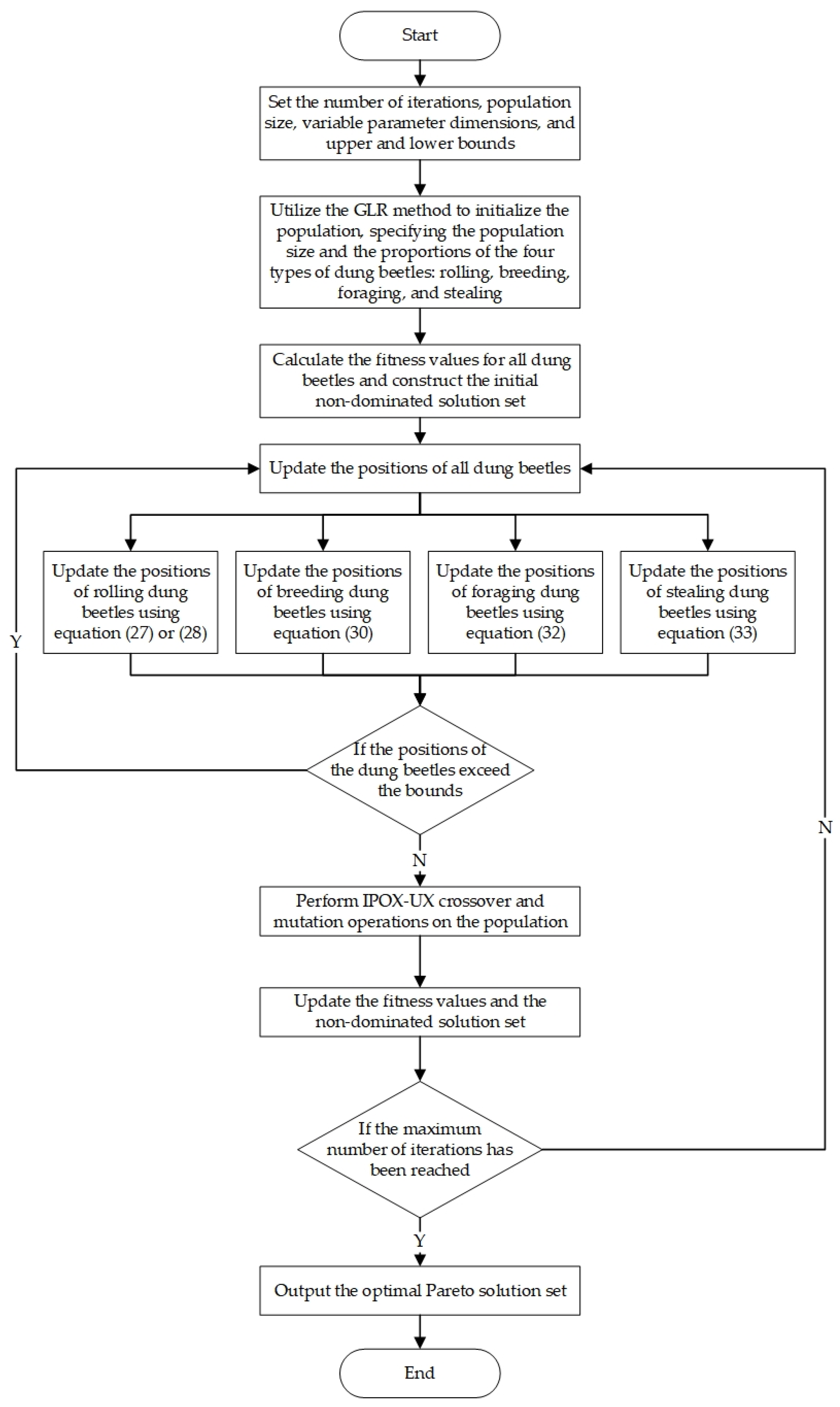
Based on the aforementioned algorithm design strategy (see details in Algorithm 1),
Figure 2 presents a flowchart that illustrates the INDBO algorithm.
| Algorithm 1. INDBO (Improved Non-dominated Dung Beetle Optimization) for Low-carbon FJSP. |
| Input: | dataset data.mat; population size ; max iterations ; crossover probability ; mutation probability ; operator proportions (GLR/IPOX/UX). |
| Encoding: | individual , where is a precedence-feasible operation sequence and is the machine assignment vector. |
| Objectives: | minimize makespan (h), total carbon emissions (), production cost (yuan). |
| Output: | nondominated set with decoded schedules and KPIs. |
| 1. | Initialize: set budgets and random seed; build precedence graph and feasible machine sets. |
| 2. | GLR-guided population: generate individuals: sample precedence-feasible ; assign by energy-aware/shortest-PT tie-breaks. |
| 3. | Decode & evaluate: serial schedule generation with machine-availability lists and insertion of setup/transport times; compute . |
| 4. | Rank: fast non-dominated sorting + crowding distance; set elite archive . |
| 5. | For do
5.1 Selection: tournament within fronts.
5.2 Crossover:
—IPOX on with prob. : copy a subsequence from Parent-1; fill the rest by Parent-2 order while preserving precedence; repair if needed.
—UX on with prob. : per operation, inherit a parent’s machine (50%); repair to feasible set if required.
5.3 Mutation: small block swaps on /feasible reassignment on with prob. .
5.4 Combine & evaluate: parents + offspring; decode & compute objectives.
5.5 Rank & elitism: fast non-dominated sorting; select next generation by fronts and crowding distance; update . |
| 6. | Return . |
| Notes. A serial SGS is employed to ensure feasibility. Per-iteration cost is ; overall complexity . |
5. Case Study
5.1. Basic Data
To evaluate the feasibility of the developed flexible job shop low-carbon scheduling model, a case study analysis is conducted using a shaft-type parts production workshop. The production unit comprises 15 processing machines, specifically including four lathes (labeled M1 to M4), three milling machines (labeled M5 to M7), three drilling machines (labeled M8 to M10), three heat treatment devices (labeled M11 to M13), and two grinding machines (labeled M14 and M15). A total of eight job types are scheduled for processing, with 20 units per job type. Each job adheres to a standard processing sequence of “turning-milling-drilling-heat treatment-grinding,” although some jobs may require only three or four operations. For each operation, machines with varying power levels are available for selection.
The processing time, operational power consumption, and average tool wear for each job and operation on each machine are presented in
Table 2. The symbol “-” indicates that the corresponding job does not require processing on the specified machine. The units for processing time, operational power consumption, idle power consumption, and average tool wear in
Table 2 are seconds (s), kilowatts (kW), kilowatts (kW) and grams (g), respectively. Jobs are transported between selected machines for various operations using an electric forklift with a rated power of 3.5 kW. The loading, unloading, and transport times between each operation and machine are provided in
Table 3. Additionally, to streamline production, machine adjustment times are established when two distinct jobs are processed consecutively on the same machine. The adjustment times for any two products processed on the same machine are listed in
Table 4. Due to space limitations, only a subset of the adjustment time data is provided. An adjustment time of 0 signifies that no processing is required on the corresponding machine.
To evaluate the carbon emissions for each stage of the job processing workshop, this study compiles and analyzes the usage costs of each machine, the consumption of cutting fluid during processing, material loss before and after job processing, and the quality of jobs during heat treatment. These data are presented in
Table 5 and
Table 6. Additionally, information regarding auxiliary facilities in the workshop is summarized in
Table 7.
The relevant coefficients for the heat treatment process in this case, which are organized in accordance with national standards, are presented in
Table 8. Additionally, the carbon emission factors associated with the resources involved in the manufacturing process are detailed in
Table 9.
The model was simulated using MATLAB R2021b, with the following algorithm parameters configured: a population size of 100, a maximum of 200 iterations, proportions for the dung beetle’s rolling, reproduction, foraging and stealing behaviors set to 0.2:0.2:0.2:0.4, GLR initialization ratio parameters set to 0.1:0.1:0.8, a crossover probability of 0.9, and a mutation probability of 0.1. All objectives are normalized to the interval [0, 1], and the hypervolume (HV) is calculated using a consistent nadir-based reference point across all methods.
5.2. Parameter Sensitivity
A one-factor-at-a-time analysis (
Table 10,
Table 11,
Table 12 and
Table 13) varies population size (P ∈ {50, 100, 200}), iteration budget (T ∈ {100, 200, 400}), mutation probability (
∈ {0.05, 0.10, 0.20}), and GLR ratio (r ∈ {0.3, 0.5, 0.7}). Hypervolume (HV) and runtime results show stable performance near the default configuration (P = 100, T = 200,
= 0.10, r = 0.5). Increasing P from 50 to 100 raises HV from 0.784 ± 0.010 to 0.800 ± 0.010 without significant runtime increase (≈45 s), while further enlarging P to 200 only yields marginal improvement (0.808 ± 0.010). These results confirm the robustness of the adopted configuration settings.
5.3. Result Discussion
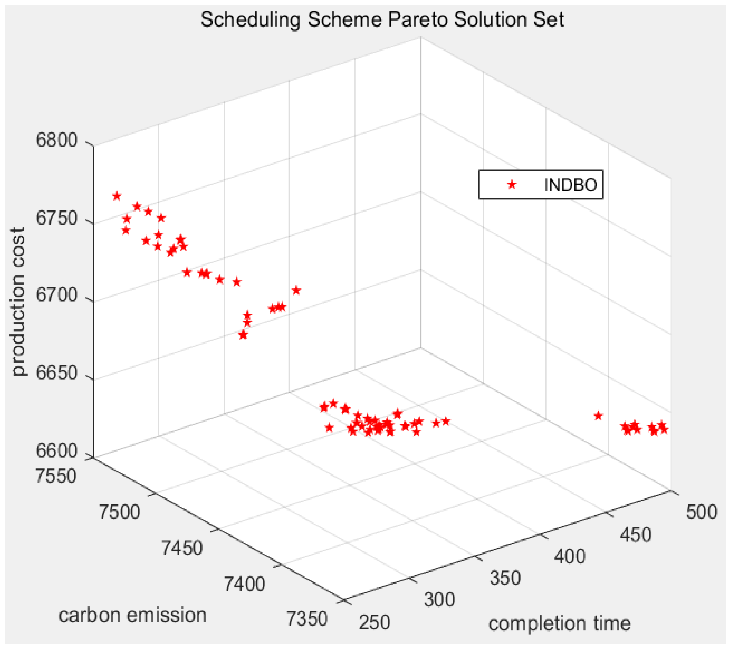
Based on the simulation analysis, the Pareto-optimal solution set for the three optimization objectives—minimum maximum completion time, minimal total carbon emissions, and reduced production cost—in the flexible low-carbon scheduling of a specific shaft-type part workshop has been successfully identified. The distribution of these solutions is illustrated in
Figure 3, while the corresponding objective function values (partial) are summarized in
Table 14.
As illustrated in
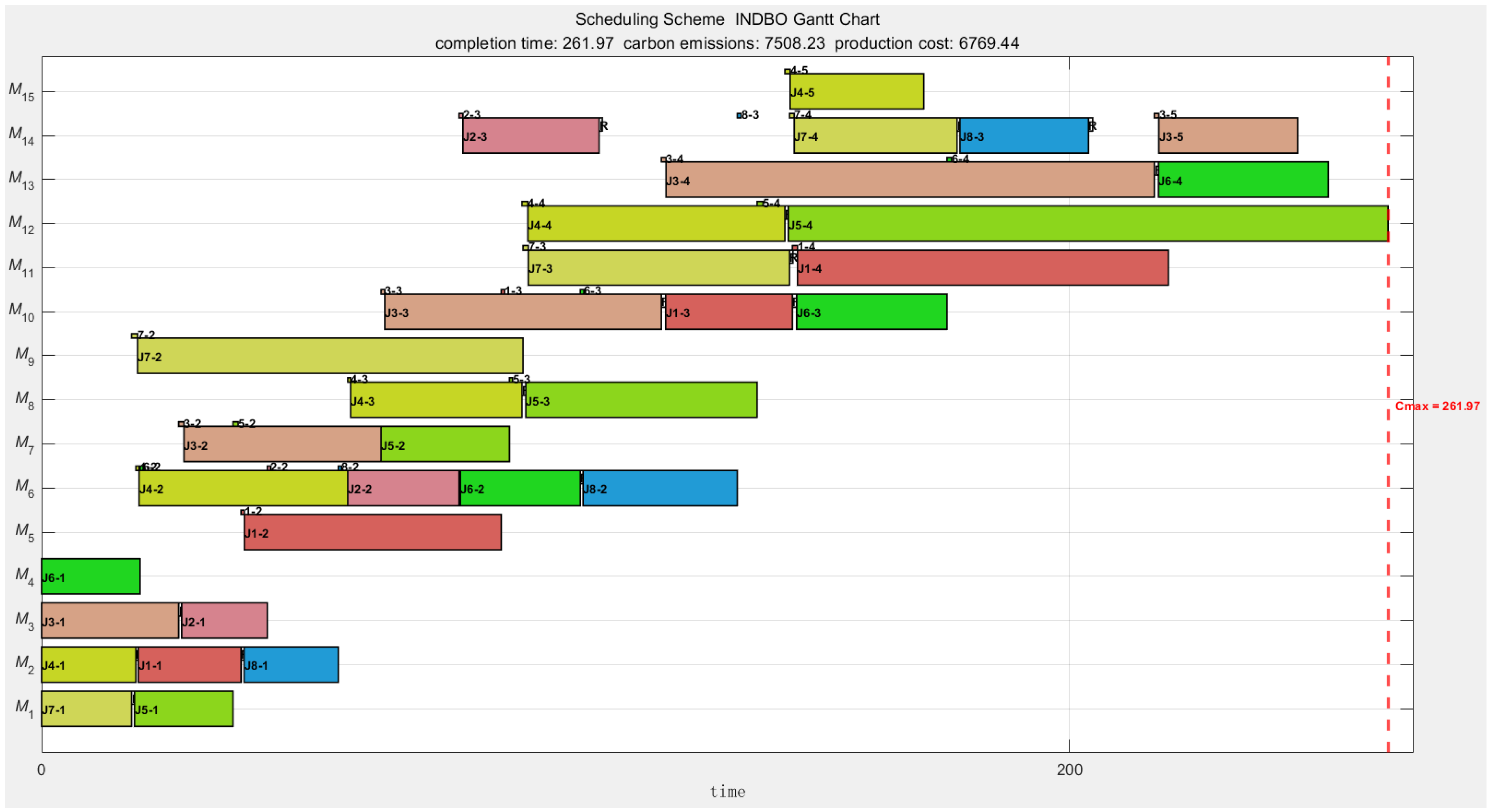
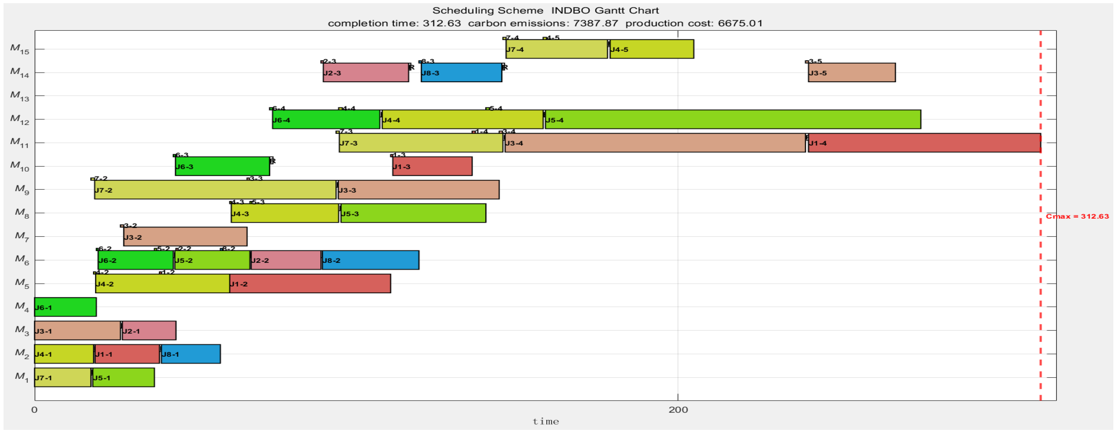
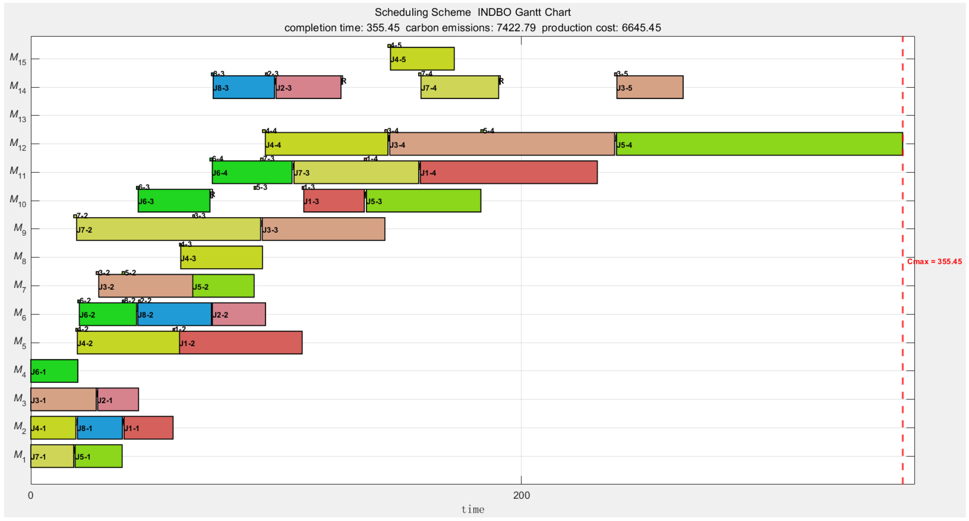
Figure 3, the objective function values within the Pareto solution set do not exhibit a clear linear relationship, indicating a lack of linear dependence among the objectives in the integrated optimization model. This feature makes it challenging to achieve simultaneous optimality across all objectives. Given the varying preferences of decision-makers in real-world applications, this study proposes three distinct scheduling strategies: efficiency-oriented, cost-saving-oriented and low-carbon environmental protection-oriented. Each strategy selects the optimal solution for a specific objective from the Pareto frontier, thereby ensuring the most appropriate scheduling alternative under the respective criterion. Specifically, solutions 1, 26 and 56 in the Pareto optimal solution set correspond to the minimization of maximum completion time (efficiency-oriented), production cost (cost-saving-oriented) and total carbon emissions (low-carbon environmental protection-oriented), respectively. Specifically, when the minimum completion time is 261.97 h, the corresponding total carbon emissions are 7508.23 kg-CO
2, and the production cost is 6769.44 yuan. Conversely, when total carbon emissions are minimized to 7387.87 kg-CO
2, the completion time increases to 312.63 h, with a corresponding production cost of 6675.01 yuan. Finally, when the production cost is reduced to 6645.45 yuan, the completion time extends to 355.45 h, and total carbon emissions rise to 7422.79 kg-CO
2.
Figure 4,
Figure 5 and
Figure 6 illustrate the Gantt charts for the respective scheduling strategies. In these charts, “J1-1” denotes the first operation of job 1, while “1–2” represents the loading and unloading handling time during the transfer of job 1 from the machine performing the first operation to that performing the second. The white square labeled “R” indicates the adjustment time required between adjacent jobs processed on the same machine; all other symbols follow a consistent labeling convention.
By comparing the Gantt charts under the three distinct strategies, it is evident that Machine 13 remains idle in both the low-carbon environmental protection and cost-saving scheduling strategies. Further analysis reveals that the processing time, process coefficient, and usage cost among the three heat treatment machines exhibit no substantial differences. However, Machine 13 has a relatively higher no-load power consumption. Consequently, when accounting for the carbon emissions and production costs associated with job transportation and machine adjustment times for M13, its disadvantages become more pronounced, leading the algorithm to exclude its utilization.
In practical applications, decision-makers can conduct a comprehensive evaluation of completion time, total carbon emissions, and production cost by considering the specific requirements of the workshop. They can assign appropriate weights to the scheduling objectives, normalize these values, and subsequently develop an integrated scheduling plan to guide production activities.
5.4. Algorithm Analysis
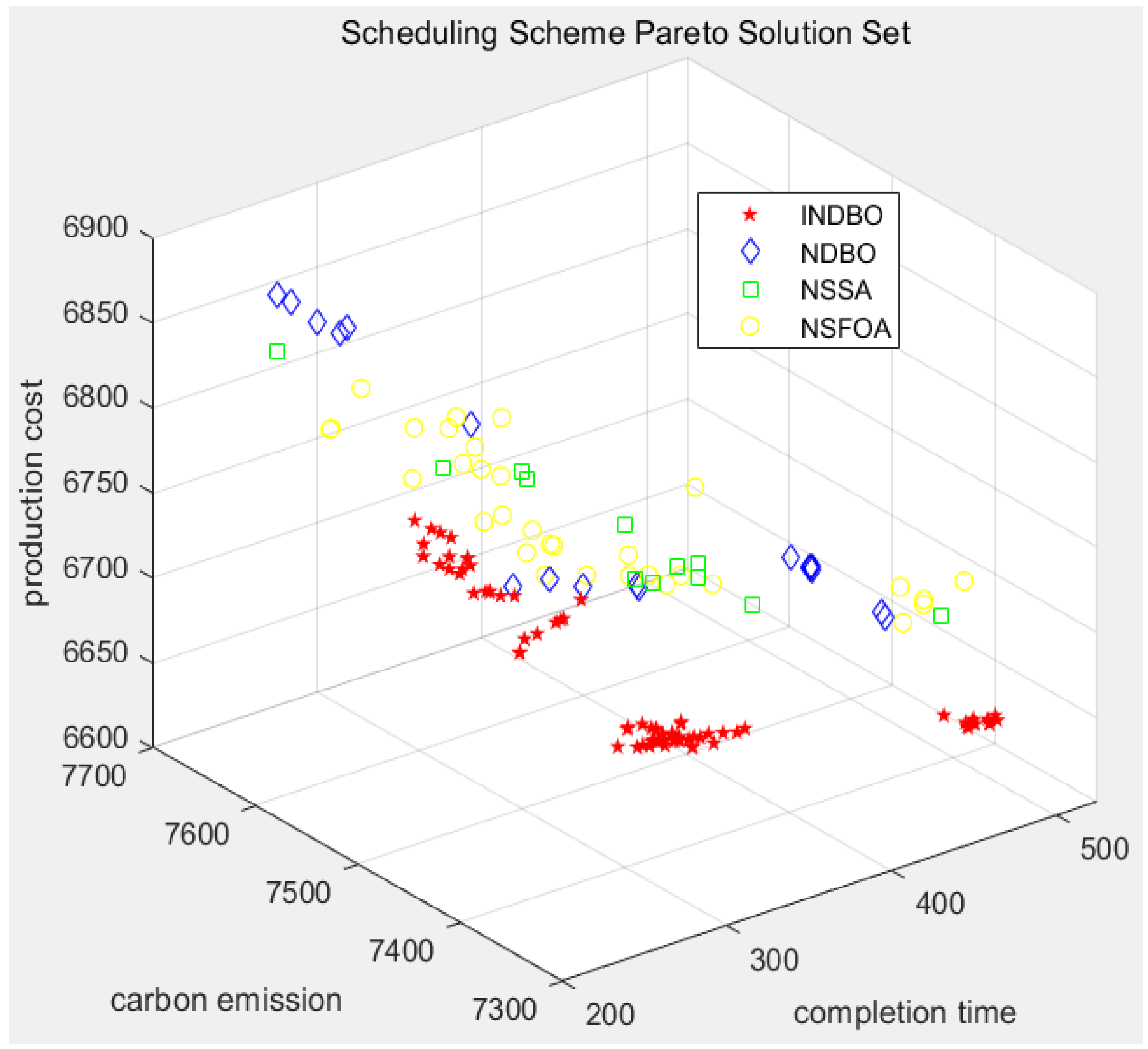
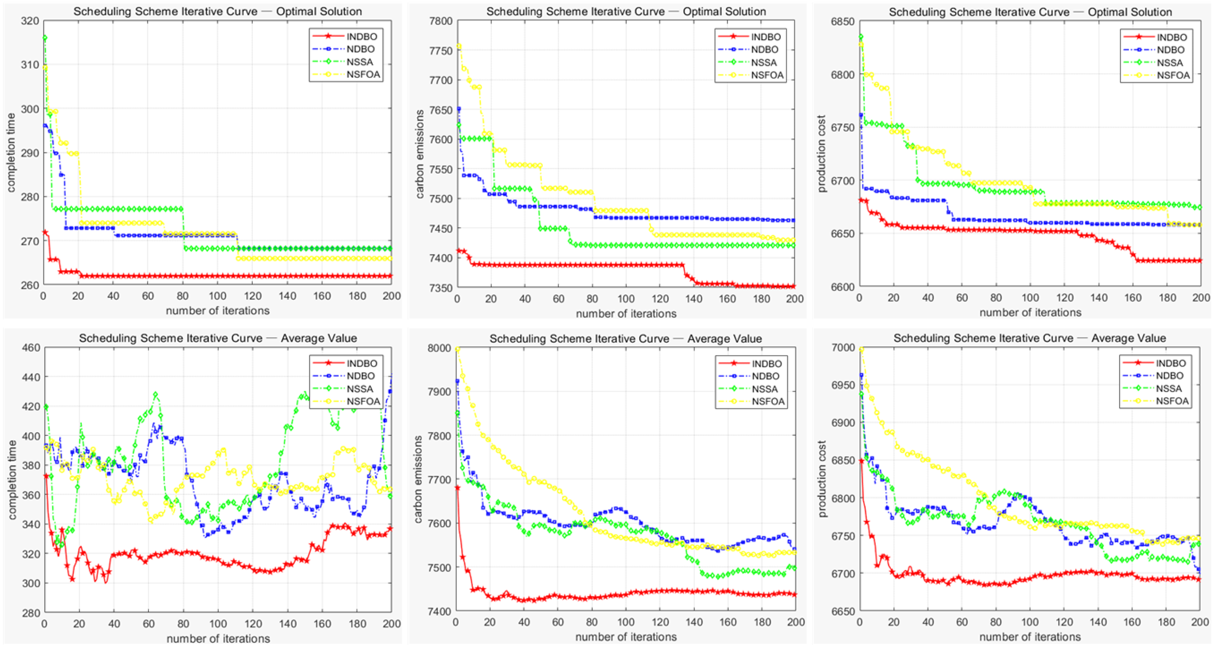
To evaluate the performance superiority of the INDBO algorithm proposed in this study, a comparative analysis is conducted against three state-of-the-art multi-objective optimization algorithms: the non-dominated sorting dung beetle optimizer (NDBO), the multi-objective sparrow search algorithm (NSSA) and the multi-objective starfish optimization algorithm (NSFOA). The Pareto solution set distributions and convergence trajectories—specifically, the best and average objective values across iterations—are illustrated in
Figure 7 and
Figure 8, respectively. Each algorithm was independently executed 30 times under identical conditions to ensure statistical reliability. Performance was assessed based on the best and average objective values, as well as the hypervolume (HV) indicator. The aggregated results are presented in
Table 15, with the best-performing outcomes highlighted in bold for clarity.
According to the aforementioned analysis, the non-dominated solution set obtained by the proposed INDBO algorithm is predominantly concentrated in the vicinity of the minimum region along the coordinate axes. This algorithm exhibits significantly superior performance compared to the benchmark methods across multiple evaluation metrics, including the optimal value, average and HV. Although it did not achieve the best performance for the optimal value of the maximum completion time objective, it still ranked second among the four algorithms, with only a marginal difference from the optimal outcome. These results collectively demonstrate that the proposed algorithm in this study possesses excellent solving efficiency and generates a high-quality solution set.
5.5. Scalability Analysis
To further evaluate scalability, larger instances up to 50 machines × 40 jobs were generated using the same configuration files. Objectives were normalized to [0, 1], and HV was computed with a fixed nadir-based reference point across all methods.
The results (
Table 16) demonstrate that INDBO achieves HV = 1.127, maximum completion time = 298.26 ± 5.21 s, total carbon emissions = 7427.39 ± 48.12 kg-CO
2, and production cost = 6682.68 ± 52.74 yuan. Runtime growth follows the theoretical
trend, indicating that INDBO scales effectively to larger problem sizes.
For large-instance performance (up to 50 machines × 40 jobs), INDBO achieves HV = 1.14 ± 0.02, IGD = 0.05 ± 0.005, and Spacing = 0.031 ± 0.004, outperforming NDBO (1.06 ± 0.02), NSSA (1.03 ± 0.02), and NSFOA (1.01 ± 0.02). Runtime increases modestly (≈ 90 ± 10 s), consistent with the theoretical O(P log P) trend, demonstrating scalability of the proposed INDBO.
6. Conclusions and Future Research
To more comprehensively evaluate the environmental impact of job processing, this paper investigates the low-carbon scheduling problem in flexible job shops. A low-carbon flexible job-shop scheduling model is proposed for a traditional mechanical component flexible job shop, taking into account factors such as loading/unloading handling time and equipment adjustment time. From an overall perspective of the job manufacturing process, the model aims to optimize three objectives: minimizing maximum completion time, reducing total carbon emissions, and controlling production costs. Considering the multi-objective nature of this scheduling problem, an INDBO algorithm is introduced to address the issue, with the following critical improvements: (1) The GLR initialization strategy is incorporated to enhance the diversity and quality of the initial solution. (2) The IPOX-UX crossover mutation strategy is adopted to effectively integrate the directional search capabilities of DBO with the stochastic exploration features of genetic operators, thereby improving its capacity to escape local optima while preserving the algorithm’s convergence rate. (3) The non-dominated sorting and crowding distance mechanisms are introduced to refine the biological behavior of DBO, ensuring effective maintenance of solution set diversity and distribution while guaranteeing excellent convergence and enhancing the algorithm’s search efficiency. Finally, the feasibility and practicality of the model in addressing various production scheduling modes are validated through case study. The superiority of the improved algorithm in terms of convergence speed and solution quality is highlighted by comparative algorithm analysis.
The model and algorithm facilitate decision-making by collecting data on machine power consumption during no-load periods, transportation times and auxiliary loads, followed by the analysis of Pareto-optimal schedules aligned with enterprise-specific priorities, such as emissions limits versus delivery deadlines. In future research, by incorporating additional factors and investigating novel methodologies, the model can be enhanced to become more comprehensive and adaptable to real-world manufacturing scenarios. Future studies can further refine the low-carbon flexible job shop scheduling model by integrating batch processing size optimization and a dynamic workshop event response mechanism. Regarding batch processing optimization, it is essential to develop dynamic adjustment algorithms that balance equipment capacity, resource availability and job priority. By extending the multi-objective optimization function of the INDBO algorithm (e.g., adding objectives for batch processing size optimization), in conjunction with an improved initialization strategy and crossover/mutation operators, collaborative optimization of production efficiency, carbon emissions and costs can be achieved. For sudden dynamic events such as equipment failure, order changes or raw material shortages, it is recommended to establish a real-time monitoring system and a rapid response mechanism driven by historical data analysis, enabling dynamic rescheduling through the INDBO algorithm. The key lies in adaptively adjusting the search strategy based on the type and severity of the event, thereby strengthening the anti-interference capability of the scheduling system. These expansion directions will propel the model toward evolving into a low-carbon and efficient production system that aligns more closely with actual manufacturing environments.
