Article

The Dynamic Interplay of Consumption and Wealth: A Systems Analysis of Horizon-Specific Effects on Chinese Stock Returns

by
Faezeh Zareian Baghdad Abadi
1,
Ali Hashemizadeh
2 and
Weili Liu
3,*
1
China Center for Special Economic Zone Research, Shenzhen University, Shenzhen 518060, China
2
Key Laboratory for Resilient Infrastructures of Coastal Cities, Ministry of Education, Shenzhen University, Shenzhen 518060, China
3
College of Economics, Shenzhen University, Shenzhen 518060, China
*
Author to whom correspondence should be addressed.
Systems 2025, 13(12), 1066; https://doi.org/10.3390/systems13121066
Submission received: 1 October 2025 / Revised: 15 November 2025 / Accepted: 20 November 2025 / Published: 25 November 2025
(This article belongs to the Special Issue Data Analytics for Social, Economic and Environmental Issues)

Abstract

This paper investigates the predictability of stock returns in the Chinese market through the lens of consumption–wealth dynamics within a broader financial system. We focus on two key state variables derived from modern consumption-based asset pricing models: the ratio of log surplus consumption (scr), from the habit-formation framework, and the log consumption–wealth ratio (cay), from the long-run cointegration framework. Using quarterly data from the CSI 300 index between 2012Q1 and 2018Q4, our system-based analysis reveals a horizon-dependent pattern of predictability. The results show that scr is a strong short-term predictor of excess stock returns, reflecting cyclical changes in risk aversion, whereas cay demonstrates superior predictive power over mid- to long-term horizons, consistent with its role as a proxy for long-run expectations. Interestingly, combining scr and cay does not improve predictive performance, suggesting that the economic mechanisms they capture are distinct rather than complementary in the Chinese market. These findings provide evidence on how interconnected macro-financial variables shape stock return dynamics, highlighting the importance of considering temporal horizons when modeling financial systems.

1. Introduction

Background

The pricing of capital assets, especially stock, in the investment process is one of the most critical issues facing investors and capital market players [1]. Pricing is closely tied to risk, which is why financial economists have developed various models for risk measurement [2]. One of these patterns is the Capital Asset Pricing Model (CAPM). The model was initially welcomed, but after a while, it was sharply criticized by financial experts. Among the models that have been extended to address the defect of the previous model, the consumption-based CAPM (CCAPM) is considerable. In the first steps, Rubinstein, Lucas, Breeden, and Grossman and Shiller expanded this model theoretically to clarify the relationship between return and risk. This model comprehended static CAPM and intertemporal CAPM by connecting equity risk premia directly to systematic consumption risk. The essential advantage of the consumption-based model is that consumption is readily measured.
The central core of various asset pricing models is constructed with a consumption growth ratio. Some researchers presented a theoretical model relating consumption to another variable named the price–dividend ratio. They argued that consumption could make a balancing connection with this ratio. This connection is the enhancement of future dividends and the enhancement of expected future interest rates due to expected future consumption growth. Additionally, since stock prices affect wealth directly, their oscillation affects consumption through a variety of possible alternative avenues. Second, growth in the value of assets in each type of investment will increase its portion of the total savings portfolio of householders. As the third reason, although asset prices do not affect consumption directly, common macroeconomic factors do drive both of them.
CCAPM employs a firm theoretical basis constructed on the financial concepts of utility maximization for pricing assets. Due to the extremely nonlinear nature and nonpartibility of consumption over time, accurate estimation is generally difficult. Nonlinear Two-Stage Least Squares (N-TSLS) is a powerful tool for explaining CCAPM problems in practical research. But selecting instrumental variables has a considerable effect on its estimates, and different sets of variables yield different results. If the variables are not chosen correctly, the results will not be reliable. When returning to standard CCAPM models, these have not been appropriately executed in practice. The results obtained from the market data of different countries show unsatisfactory results. Researchers modified consumption-based CAPM to produce more reliable empirical results in order to estimate international stock market returns.
China’s financial system has changed quickly, and there have been ongoing changes to make the market more efficient, raising foreign investment, and deepening connections between the macro and micro levels of finance. As the world’s second-largest economy, it is important to understand how return predictability works in the Chinese stock market [3]. This is important for both local asset pricing research and worldwide investment allocation. Consequently, these are our motivations for selecting the Chinese stock market as a case study for a study on the consumption-based CAPM. Although many types of research contribute to the literature on CCAPM, attention to the Chinese market has been much lower than its importance. China is the primary driver of world trade, economy, and export and import [4]; therefore, this country’s stock markets have received enormous attention in theoretical and experimental research [5]. China’s institutional and investor properties are unique, and experts have examined different aspects of the Chinese stock market. But capital pricing models for this market need further research and investigation. In this research, we aim to address the shortage of the related literature and investigate the power of CCAPM in explaining excess returns in the Chinese stock market. For this, two consumption state variables have been used, including the log surplus consumption ratio (called scr), and the log consumption–wealth ratio (called cay). The CCAPM approach and long-run hazards frameworks, have undergone extensive testing in developed countries; nevertheless, empirical data in significant developing markets are still scarce. This difference is particularly significant in China, where distinctive institutional characteristics, changing market involvement, and policy-induced liquidity cycles might modify the interplay between consumption, wealth, and anticipated returns. Our work enhances CCAPM research by investigating whether surplus consumption (scr) and the consumption–wealth ratio (cay), two theoretically based state variables, provide unique and horizon-dependent prediction information for stock returns in China.
Our study enhances the literature in several aspects. The capacity for consumption growth is fundamental to several asset price models. Certain academics proposed a theoretical model that connects consumption with the price–dividend ratio. They contended that consumption may exhibit an offsetting connection with this ratio, in which heightened anticipated future consumption growth elevates projected future dividends while concurrently raising expected future interest rates. Moreover, stock prices are thought to influence consumption via other potential channels. This may mostly be seen via a direct wealth impact. Secondly, an appreciation in the asset prices of a particular investment or savings vehicle will augment its proportion within a household’s overall savings portfolio. Third, asset prices may not directly influence consumption; rather, both may be influenced by a shared macroeconomic component. This research enhances the current literature by using stock returns rather than portfolio returns as the dependent variable. The primary variable for this study is consumption, with size and inflation serving as control factors. This study employs applied research to ascertain the correlation between consumption and stock returns using statistical parameters, utilizing empirical data from the China stock market.

2. Literature Review and Hypothesis Analysis

2.1. Consumption-Based CAPM

The topic chosen to be covered in this research is the study of a consumption-based asset price model using the Chinese stock market. CCAPM is an essential topic in financial issues. As a matter of fact, researchers in the field of economics have also made great efforts to provide such a framework. The ability of CCAPM models to explain asset prices and business cycle data at the same time has advanced significantly in recent decades [6]. A consumption-based CAPM was initially suggested by Lucas and others. They established this model to connect the consumption rate to the excess stock market [7]. Risk is the principal factor of diversity in expected asset returns. Quantifying risk accurately is a crucial first step in risk management, and this entails calculating correlations and volatility throughout the whole investable asset universe [8]. The commerce volume and transaction expenses can be relinquished in these models. To define the relationship between risk and return, these factors are assumed as [9]:
E(Ri) = Rf + βi (RmRf)
where E(Ri) is the expected return investors desire for the ith asset; Rf is the return of the risk-free rate, calculated by period average background; Rm is the return of the market portfolio, calculating by risk and the period average background; and βi is a systematic risk measurement for the ith asset.
The following describes these assumptions:
  • Many adequate investors are price-takers;
  • The investment period is the same for all investors;
  • Taxes and transaction costs are ignorable;
  • The risk-free rate is a real reference rate for borrowing and lending;
  • Expected return and variance have the most attention from the perspective of investors;
(a)
A high mean and low variance are preferable;
(b)
The market included all generally exchanged assets.
Vendrame et al. (2018) [10] examined various variables to demonstrate their power for predicting stock returns. Among the tested variables, three variables, including the price–dividend ratio, the default spread, and the term spread, have been displayed to present better performance. Such variables are linked with the business cycle. Therefore, it is concluded that the expected return and risk premiums change during the trading cycle. They argued that most changes in the ability to predict returns were due to changes in risk premiums, not betas. Furthermore, it is necessary to focus on time variation in risk premiums [10]. Some researchers like Fama and French, Campbell, and Hodrick provided essential pieces of evidence that the aforementioned variables can account for the time variation of returns. However, some evidence of the inability of the price–dividend ratio to predict expected returns led to other variables being considered and tested to identify new predictor variables [11]. As an example, Boudoukh et al. (2007) explained that the net payout ratio brings more satisfaction because it more accurately records the amount of money distributed to shareholders and showed that it is more suitable for estimating future returns [12].
Therefore, we considered the dividend yield to determine whether it has any proper power for predicting consumption growth. The use of the mentioned variable has not been proposed recently and was suggested in Campbell and Schiller’s proposed model; they based their research on claims that dividend yields in the late 1990s overestimated the value of the stock market. Similar arguments are seen in Rapach and Wohar who explained the behavior of dividend yields, and also investigated the reasons for their deviation. Additionally, Campbell and Shiller (1988) proposed a model that can expand the value proposition model for stock prices to cover a component of market sentiment, allowing prices to deviate from principles [13,14].
The consumption-based CAPM assesses assets based on their exposure to the risk of macroeconomic factors; unlike the traditional CAPM, which only judges their returns against the returns of other assets. The method in question thus establishes a connection between the financial sector and the economy at a tangible level. Given its principles, assets that exhibit positive growth in consumption are less noteworthy to decision-makers because they do not provide security in difficult situations. Hence, investors must be compensated with the expected return on this kind of asset. Despite the correct methodical basis, empirical support for the standard CCAPM in terms of describing stock returns is brittle and unreliable [15].
There are different interpretations of CAPM pricing rules based on consumption. For example, some researchers have claimed that the price of an asset with a random repayment is less than the expected repayment, while a random repayment is directly related to consumption. Although this interpretation of the CCAPM pricing rule is not theoretically complete, there is considerable evidence to support it, and it must be acknowledged to be right given some additional conditions [16].
Chang et al. (2019) [17] contributed to the body of research on consumption-based CAPM, building on the work of Lettau and Ludvigson (2001) [18] regarding the cay and the prediction of equity market variations. They accomplished this by (a) employing time-varying cointegration techniques to establish a time-varying index of the consumption–aggregate wealth ratio (cayTVP); (b) evaluating the predictive efficacy of the cayTVP measure against that of the cay and Markov-switching cay indices concerning excess stock returns and volatility in the United States from 1952:Q2 to 2015:Q3; and (c) examining the predictive capacity of the three indicators of the consumption–aggregate wealth ratio utilizing a nonlinear causality-in-quantiles test developed by Balcilar et al. (2017) [19]. They discovered that there is cointegration between labor income, asset wealth, and consumption, although in a time-varying manner. Generally speaking, cayTVP is significant in bear markets, cay performs well in normal to excellent market conditions, and cayMS typically performs well in bull markets and in periods of relatively bad performance. They thus came to the conclusion that, depending on the situation of the stock market, investors may learn valuable information from all three metrics [18,19].
Adhering to the well-known consumer-based CAPM, the over-performance of a market portfolio is a popular parameter that illustrates discrimination in cross-sectional returns. Labor income and consumption increase have perfect connections [20]. Marquez et al. (2014) [21] proposed a fundamental consumption-based model. Despite other models in asset pricing research that focus on cumulative liquidity risk, their proposed framework is implemented by answering the representative customer–investor improvement challenge based on the idea of general consumption risk. Their best outcomes were obtained for their proposed framework under the ultimate risk characteristics.
Despite the standard CCAPM being deducted from the power utility, where the single parameter is consumption growth, it can improve the performance of the consumption-based model by comprising two factors, which are called innovation in market returns and innovation in consumption growth. It is possible to overcome a popular indictment of the mentioned model, in which the marginal utility of consumption is based only on current data on consumption. Then, the marginal consumption utility becomes a function of both consumption growth and the returns of the market [15].
In another study, Jacobs and Wang tested the importance of the idiosyncratic risk of consumption for cross-sectional changes in asset returns. These researchers understood that cross-partial variance in consumption increase and total growth rates were both important pricing parameters. The outcomes they obtained proposed that two-factor CCAPM outperforms the CAPM. Additionally, it performed nearly like the Fama–French three-factor framework [22].

2.2. Chinese Stock Market

China has a distinct environment in different aspects, such as social, economic, and cultural, in comparison with other countries of the world. Additionally, it has grown significantly in global trade and international commerce as a consequence of its enormous development [23]. China is the most prominent driver of the world economy and international trade by leading imports and exports around the world. Hence, all of the aspects of the economy of China (such as the Chinese stock market) are desirable areas to which experts and researchers can extend theoretical and empirical studies. Due to its unique institutional and shareholder properties, experts have explored its stock market from many various points of views. This includes the Shanghai stock exchange and the Shenzhen stock exchange. Recently, as China’s economy has grown, so has its stock market [24]. This market has considerable differences compared to the U.S. market. The main difference is that the estimated high risk is due to the low correlation between the macroeconomy and the stock market in China, not the low volatility of market returns as in the United States [25]. Undoubtedly, determining the factors affecting stock returns in the volatile Chinese stock market is considerably more difficult [26].
The consumption pattern in China is another significant issue to consider when analyzing the stock market. People with less economic and financial knowledge may not reduce their consumption as their wealth and income are impaired. On the contrary, individuals with good financial literacy should strive to mitigate unexpected losses and adjust their consumption to align with the current situation. As a result, they are more susceptible to behavioral biases and market disruptions. Hence, heterogeneous household characteristics influence the decision-making process in consumption [27].
Focusing on this, Huang (2018) [28] compared the outcomes of traditional CAPM, including four different models. The four types are the Sharpe–Lintner CAPM, the Fama and French three-factor model, the Fama and French five-factor model, and the Carhart four-factor framework. The five-factor model is generally more effective than other models in terms of depicting the individual returns of Chinese stock markets. However, the inclusion of investment and profitability components only marginally enhances the model’s outcomes, suggesting that both factors possess a maximizing effect but little explanatory power regarding stock returns. By calculating whether equity return dispersion, which is determined by the cross-partial normal deviation of stock returns, bears a significant price risk, Chen et al. (2015) [29] expanded on empirical research on asset pricing analyses for the markets in question. Even after controlling for market, size, book-to-market, and idiosyncratic volatility impacts, the investigators noted that stock return dispersion is really systematically priced in the cross-section of returns in this improving market.
Le et al. (2025) [30] examined the impact of investor regret on asset prices within the Chinese stock market using data from 2000 to 2021. They concluded that equities related to increased investor remorse often provide better future returns. This study emphasized the influence of behavioral variables, such as regret, on stock values, particularly in developing markets like China. Given the complicated and sometimes contradictory outcomes in the previous research on assigning stock returns in China, the dispersion of stock returns as a systematic risk ratio presents a more significant proxy for risk in this improving market, where many aspects have changed dramatically [29]. Table 1 summarizes some research about the Chinese stock market and the stock markets of some other countries.
Researchers have examined CCAPM in developed markets extensively; however, research on its application to China’s distinctive stock market context remains scarce. China’s market is distinctive because it has a lot of individual investors, people who do not know much about finance, and policies that change all the time. These things might modify how consumption and wealth connect to stock returns. Previous research has seldom analyzed the functionality of state indicators, such as the scr and the cay, over various temporal periods in China. Moreover, several prior studies inadequately addressed critical concerns such as structural fractures in the market and potential endogeneity among variables, and failed to conduct comprehensive diagnostic testing to guarantee dependable outcomes. We address these shortcomings in this research by using a CCAPM framework that incorporates scr and cay, utilizing sophisticated techniques to manage endogeneity and dynamics, and rigorously evaluating the model’s validity via diagnostic assessments. This method helps us learn more about how stock returns are affected by wealth and consumption in the changing Chinese market.

2.3. Hypothesis Development

Even though the consumption-based CAPM significantly reduces the pricing errors of the portfolio-based framework, the standard strength utility CCAPM and the HF-CCAPM are able to describe the cross-partial variation in equity risk premia, whereas the CAPM is unable to do so. The power utility CCAPM can account for over 50% of the change in risk premia, and the habit formation model can account for over 90%. Therefore, according to Auer (2013), consumption-based parameters that include the surplus consumption coefficient and the consumption enhancement rate are important indicators [35].
In another study, Chen and Ludvigson state that habit formation models provide a very good explanation of the overall behavior of the stock market when it comes to the content of equilibrium consumption. The most notable habit model was extended by them. According to this hypothesis, individuals progressively broaden their purchasing patterns, making risk aversion anti-cyclical and changeable over time. The significant US equity premium for the US stock market may be explained by the model. One feature of the framework is that, although the risk-free rate is small and steady, the average risk aversion over time is significant. Therefore, without taking the risk-free rate into account, the suggested framework resolves the equity premium problem with considerable risk aversion. The enhanced consumption-based CAPM can forecast returns in global stock markets. Li and Zhong (2010) [22] investigate consumption-based CAPM with habit development, prediction, and the cross-partial of returns from global stock markets using quarterly data collected from 17 different nations. They asserted that the returns from the majority of established equity markets could be accurately described by the local and global stock markets. Their cross-partial analyses of CCAPM in habit development state that the model performs better than a three-factor international model comprising the unconditional global CCAPM, CAPM, and the conditional world CAPM. Thus, the following theory is taken into consideration:
Hypothesis 1:
The scrt significantly predicts future stock returns and assumes that expected returns are inversely related to scrt.
A cointegration relation between log labor income (yt), log asset holdings (at), and log consumption (ct) was discovered by certain researchers, and the CAYT model they generated may predict excess returns on the U.S. stock market across short and intermediate time horizons. Additionally, cross-sectional stock market returns may be described by cayt in CCAPM. Additionally, they contrasted its implementation outcomes with those of the Fama–French three-factor framework. Li and Zhong (2010) [22] discovered a positive linear association between cayt and the extra stock market return. According to McMillan (2013) [13], there is a strong relationship between dividend yield and consumption enhancement; hence, when the dividend yield is low, spending is high. Through predictions about future economic behavior, he contended that there is a steady association between the current dividend yield and future spending. Then, in order to predict future stock returns, it is necessary to combine the cayt and the expected future growth in labor income. This will demonstrate that not only do the anticipated changes in labor income have a high degree of predictability in terms of future returns, but that the combination of the cayt and expected changes in salaries accurately describes the change in the cross-section of returns. In the long term, however, the dividend yield responds to anticipated future behavior. According to him, there is a clear correlation between the effect of income from modern stock returns and increased spending. He did point out, nevertheless, that the positive coefficient’s statistical significance varies throughout the six models. Ultimately, he focused on single-market regressions, even though the main result relies on panel estimation [13]. The following theory is then taken into account:
Hypothesis 2:
cayt significantly predicts future stock returns and assumes that the expected returns are directly associated with cayt.
If consumption adheres to a random walk process, the wealth-to-consumption ratio in the consumption-based framework with habit formation should only rely on the consumption-to-habit ratio. Moreover, anticipated stock returns ought to vary only with delayed habit-based consumption if dividends and consumption adhere to random walk processes. Consequently, an inherent correlation should exist between the coefficients of wealth to consumption and consumption to habits, with the consumption–habit ratio elucidating the wealth–consumption ratio’s ability to predict stock returns. Nevertheless, evidence indicates that consumption increasing is serially correlated, despite actual data often corroborating the random walk theory for dividends [36]. Thus, the following theory is taken into consideration:
Hypothesis 3:
The cayt and scrt are supplementary and have more predicting capacity than single-state variables.

3. Data and Models

3.1. Data

As discussed in the previous section, the critical state variables for the study of the consumption effect in stock returns are the scr and cay. As we have two crucial state variables, in this section, we define how the required data and measurements are collected. Our data includes macroeconomic data and other financial data. In China, the National Bureau of Statistics of China (NBSC) maintains a proper database of macroeconomic data. Online websites and the Wind database are employed to make a consumption and disposable labor income framework. These variables are time series in quarterly terms. For wealth data, we searched many local and international sources, the best available sources being the information supplied by the CREDIT SUISSE GROUP. This information is published each year. Here, we used the data from 2012Q1 to 2018Q4. In this period, there are 28 observations. The quarterly data used, and data covering other time periods, are adjusted to fit real per capita data.
There are three reasons why this period was selected. First, it shows a time of major changes in the market that were meant to make it more open, provide more people access to it, and encourage growth based on consumption. Second, during this time period, solid and regular quarterly data on household wealth and spending became accessible. Third, the window leaves out the huge changes that happened during the global financial crisis of 2008–2009 and the COVID-19 epidemic. This lets us concentrate on fundamental macro-financial interactions instead of crisis-specific aberrations.
We have chosen the CSI 300 as our stock market index since it is one of the most widely utilized indexes. One such stock market index is the CSI 300, which attempts to reflect the performance of the 300 most heavily traded companies on the Shanghai stock market by using capitalization as an indicator. The China Securities Index Company, Ltd. is responsible for compiling the index. Quarterly data was used. For the period beginning in 2012Q1 and ending in 2018Q4, we retrieved CSI300 statistics, the risk-free rate, dividend yields, dividend payout coefficients, and TRM from the RESSET database.
In our research, we use the Campbell and Cochrane external habit according to Li and Zhong (2010) [22] and Bianchi et al. to provide estimates of the surplus consumption ratio and consumption–wealth coefficient [37,38].

3.2. Variable Selection and Measurements Ratio

We have three kinds of variables including the following:
  • Dependent variable: excess return (rt);
  • Independent variables: scrt and cayt;
  • Control variables: dividend yield (dpt), dividend payout coefficient (det) and government bond term spread (TRMt).

3.2.1. Dependent Variable

Excess return is a dependent variable: rmt is the log real return of the stock market ratio, and rft is the log real return on the risk-free coefficient, therefore rt = rmt − rft.

3.2.2. Independent Variables

In this way, scrt and cayt are independent variables. As for the measurement of scrt Campbell and Cochrane explain the existing CCAPM with external habit formation. Therein, surplus consumption is specified as
S C R t = C t X t C t
where Ct is defined as the per capita real usage, and Xt is defined as an external habit level that is obtained from previous consumption terms.
cayt contains human capital and household asset holding at time t. Integrated wealth, exclusively human capital, is not directly visible. So, to predict asset returns, we must identify an agent for human capital. We utilize after-tax labor salaries as a proxy for human capital as follows:
cay t = c t β a a t β y y t

3.2.3. Control Variables

The considered control parameters are dpt, det, and TRMt. Table 2 introduces these variables.
With these in mind, we establish a model to examine our hypothesis in Section 2.3. There are two approaches to forecasting expected returns. The first approach is analyzing their relationship with one state variable. As we have two state variables, such as scrt and cayt, based on the first approach there two formations, including the only scrt and only cayt [13,39].
The formula for the expected excess return on an asset with scrt is
E t   [ r i ، t + 1 e ] = α + α 1 z t + β 1 s c r t + M A 1 + M A 2
where z t represents the vector of control variables, the slope ratio ( β 1 ) is constant, and MA1 and MA2 are moving average indicator models.
The return predicting regression equation with cayt is as follows:
E t   [ r i ، t + 1 e ]   =   α + α 1 z t + β 2 c a y t + M A 1 + M A 2
where α is stable, α 1 represents the vector of continuous slope ratios of control parameters, β 2 is the continual slope coefficient, and MA1 and MA2 are moving average indicator models.
If the expected returns are inversely related to scrt and directly associated with cayt, then Hypotheses 1 and 2 are established. The second approach is exploring this with two state variables [22]. Combining both state variables is matched with this approach. The equation of regression can be declared as
E t   [ r i ، t + 1 e ]   = α + α 1 z t + β 1 s c r t + β 2 c a y t + M A 1 + M A 2
where α is stable, β i is a stable slope coefficient, and MA1 and MA2 is moving average indicator models.

3.3. Descriptive Statistical Analysis

The fundamental descriptive statistics for the independent, dependent, and control parameters are declared in Table 3, which was taken from “Eviews.” Log excess returns on stock market indexes r, dpt, det, TRMt, scrt, and cayt are among the quarterly variables.
The correlation matrix (Table 4) indicates that the relationship between excess returns on the stock market and scrt is negative, and the relationship between excess returns on the stock market and cayt positive, which is consistent with Hypotheses 1 and 2. The described state factors scrt and cayt are softly associated with several control variables; furthermore, we orthogonalize the control parameters to the state factors in the next section and examine their predicting power.
Univariate summary statistics suggest that, on average, the change in scrt is less than that in other variables, and the difference in cayt is greater than in other variables. Regarding the autocorrelation of the parameters at the first lag, all other variables except cayt display much more autocorrelation. The high stability of the independent factors may be useful for predicting excess market returns in the long term.
The stationarity of the expected return should be checked. For this purpose, we examined our null hypothesis (the expected return is stationary) by observing its trend in Figure 1 and the KPSS unit root test. LM-stat is lower than crucial values, and we cannot reject our null hypothesis. Therefore, it is stationary.
We employed the unit root test, which is augmented by Dickey-Fuller in the series on household consumption (M1), net household wealth (M2), and disposable income (M3). We examined every one of these three series, and there is one unit root with a maximum of 6 lags for the Schwarz Info Criterion (SIC) (See Supplementary Materials Tables S1–S3).
As these three variables (M1, M2, and M3) are non-stationary, this research examines the existence of cointegration correlation between the mentioned variables. So, we utilize different types of cointegration experiment: one of the tests is the residual-based cointegration test developed by Phillips and Ouleiaris to determine whether the parameters under consideration are cointegrated, and the other is Johansen’s maximum eigenvalue test and trace statistics experiment that shows how many cointegration vectors there are in a long-term relationship. Both experiments indicate that, between the three variables, the cointegration vector is unique. The outcome of two tests, the Phillips–Ouliaris cointegration test and the Johansen cointegration test, is presented in Tables S4 and S5. Cointegration experiments show that there is a common trend between M1, M2, and M3. If we want to use cayt to test its predictive power regarding stock market returns, first we must calculate the factors of cointegration relevance. To examine endogenously specific nature of the ct, at, and yt series, Stock and Watson present a single-equation procedure and use the DLS, which refers to the dynamic least squares presented by Newey and West. The dynamic least squares (DLS) are specified as
c t = α + β a a t + β y y t
The estimation obtained from Equation (4) generates an extremely consistent estimate of β and the β of the cointegration factors [17]. We used quarterly data from 2012Q1 to 2018Q4 to compute ratios of the trend deviation of the constant, net asset wealth (at), and labor salaries (yt) from ‘Eviews 9’, which is shown in Equation (8).
c t = 14.355 + 0.9718 a t 3.9758 y t ( 10.155 )   ( 12.783 )   ( 8.828 )
Relevant t-statistics are written under the ratio in the parenthesis. From the estimation of Equation (7), we can estimate that cayt = c t β a a t β y y t . Thus
c a y t = c t 0.9718 a t + 3.9758 y t
The expected excess return on asset for both state variables can be written such as:
E t   [ r i ، t + 1 e ] =   α + β 1 s c r t + β 2 c a y t + M A i
where α is constant, βi is constant slope coefficients and MAi is moving average indicator modeling. With this in mind, for modeling, we used three different tests, including Akaike, Schwarz, and Hannan–Quinn. These methods have suggested that MA (2) is the best model for forecasting. Using MA (2), the moving average aligns with both theoretical and empirical research that shows how changes in consumption and wealth spread slowly across the financial system [40]. This specification of the moving average accounts for lagged responses in household spending, smoothing, and risk perception, enhancing fit compared to AR alternatives. Additionally, in this research, Nonlinear Two-Stage Least Squares (N-TSLS) was employed to mitigate any endogeneity between state variables and predicted returns [41]. This approach gives consistent estimates by modeling how the dependent variables of this research interact with predictive regressions. This is critical since both are forward-looking indicators that are affected by market expectations.

4. Results

4.1. Surplus Consumption Ratio

Our goal is measuring the predictability of scrt and cayt and control factors for unified stock market returns in the short and long term. We have three control variables, including dpt, det, and TRMt.
Table 5 shows the OLS regression calculation outcomes with the single state variable scrt/with control variables. The regression outcome is shown in columns (1) and (2), respectively.
The coefficient of correlation of scrt is negative, which shows that its relationship with the expected return is inverse, and Hypothesis 1 is established.
Then, we run root mean squared error (RMSE), applying a complete sample to the horizons between 1 and 14. The intended dependent factor is cumulative K-period excess market returns: Σrt+1. Table 6 indicates the outcomes of the regression using surplus consumption/with control variables. Each control factor is orthogonalized to the state variable by using the fitted residuals from the regression of the state factor. Table 6 also reports the Theil Inequality Coefficient (TIC). The lower the amount of RMSE and TIC, the better. This is also shown in Figure 2.
Our findings show that the RMSE of scrt (Regression 1) at short horizons has the best performance with the lowest value (0.023192). It matches with the theory. After that, it increases from about 0.12 (2nd quarter) to 0.14 (7th quarter), such that the highest value is 0.15 (6th quarter). This shows does not exhibit proper performance in the mid-term horizon. Regarding the long-term horizon, decreased from 0.14 to 0.11, which shows its performance becomes better over the long-term horizon than mid-term. The TIC approach is similar to RMSE in this regression. In the second regression, including scrt and control variables, RMSE is a continuously decreasing series (1st to 14th quarter), which shows this regressor is more robust with control variables. Its TIC approach is similar. Regressions (1) and (2) further validate Hypothesis 1.

4.2. Consumption Wealth Ratio

In an identical manner to the previous section, Table 7 shows the OLS regression calculation outcomes with a single state variable: cayt/with control variables.
The coefficient of correlation of cayt is positive; that means its relationship with an expected return is direct, which verifies Hypothesis 2. The Heteroskedasticity Test of all estimations was conducted according to the Breusch–Pagan–Godfreyof method. The results show that the estimations are homoskedastic (see Tables S6 and S7).
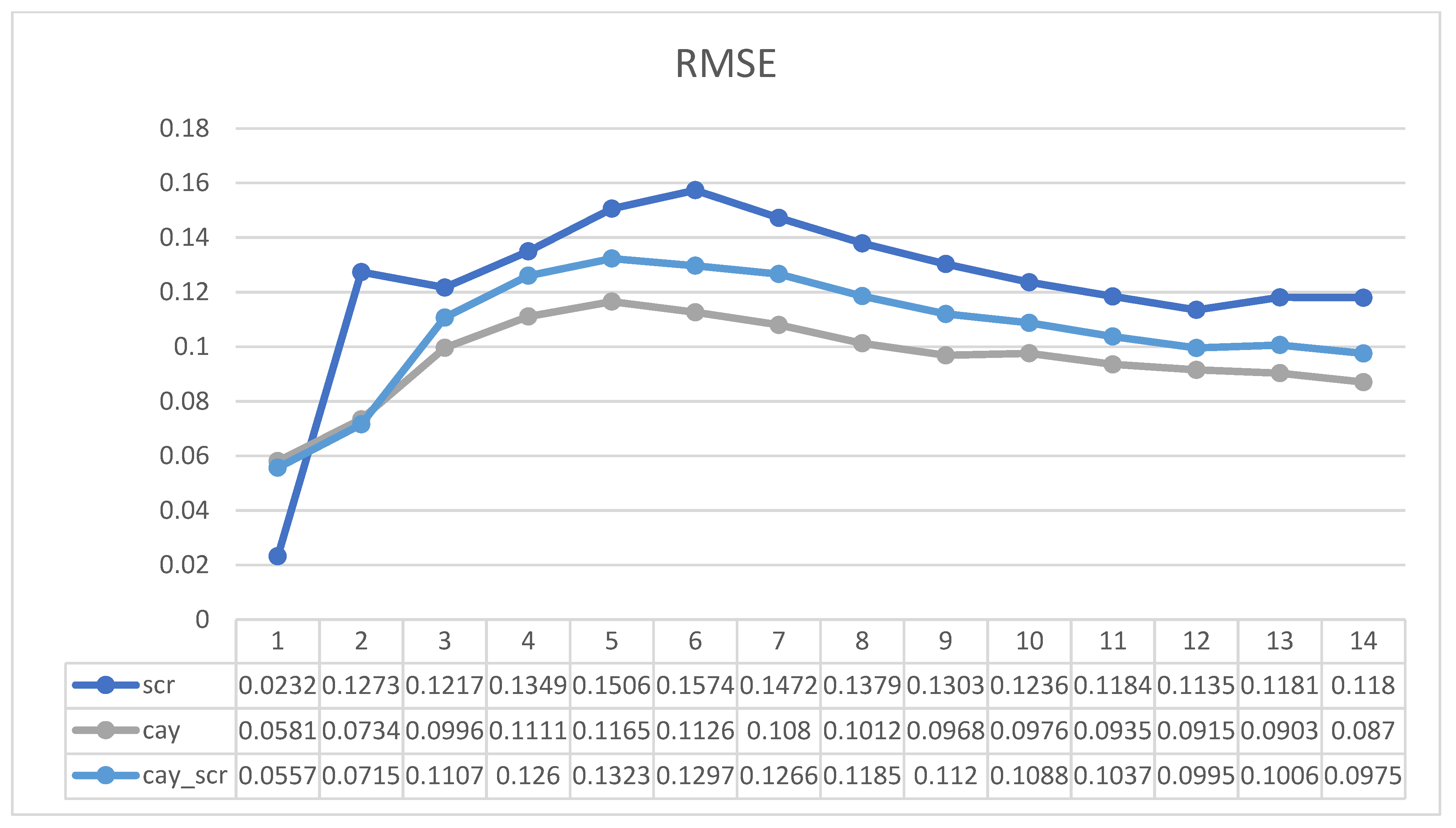
Table 8 indicates the outcomes of the regression using the state variable/with control variables. This table also reports the Theil Inequality Coefficient (TIC). The lower the amount of RMSE and TIC, the better. This is also shown in Figure 3.
In regression 3, the best performance occurred in the first step (0.058083). From the 2nd to 7th quarter, all of the RMSEs increase from 0.073398 to 0.107989. This increase in RMSE shows this regression is not so dominant in mid-term forecasting. For long-term forecasting, the 8th to the 14th quarters show that this regression is more suitable for forecasting than it is for the mid-term horizon. The TIC approach is similar to RMSE.
In the last regression, cayt with control variables, its approach from the first to last quarter is decreasing; in comparison with cayt (regressor 3), this shows that it is not more suitable forecasting. The approach of TIC in this series is similar to RMSE, which is in line with Hypothesis II.

4.3. Two-State Variable

In this section, we examine a two-state variable forecasting regression in a similar manner to the preceding section. Table 9 shows the return estimation results using scrt-cayt/with control variables. Also, the Heteroskedasticity Test using the Breusch–Pagan–Godfreyof method and the relevant correlations was conducted so that they were satisfied (see Table S8).
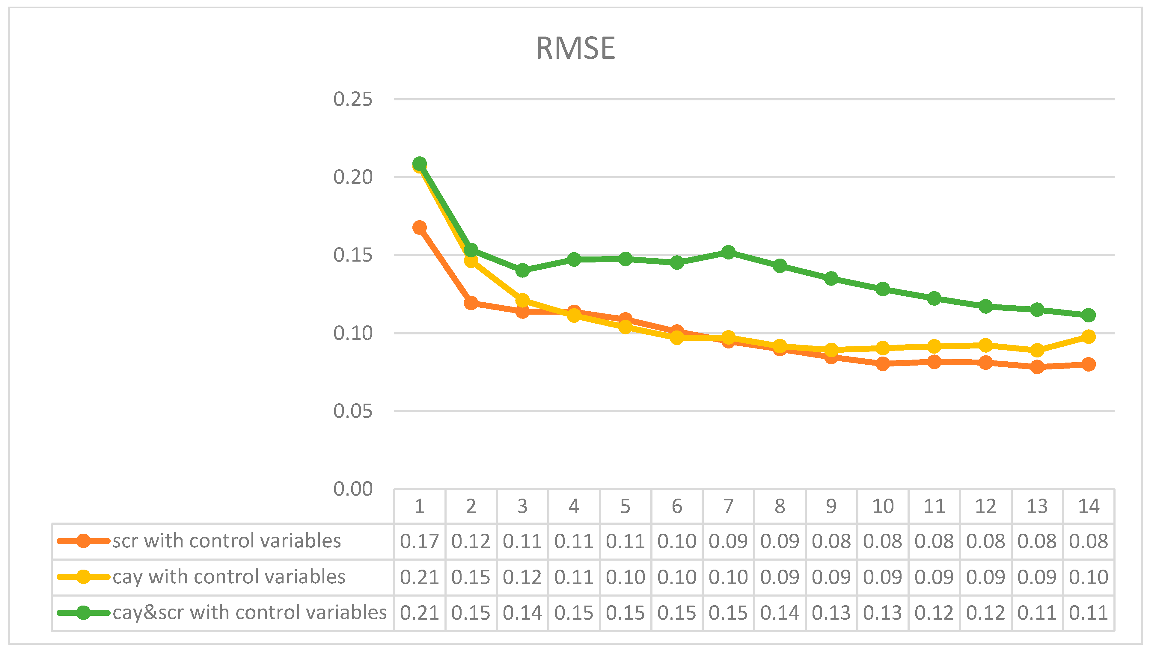
In this part, we analyze regressions, including two-state variables, using RMSE and TIC. Table 10 shows the RMSE and TIC using scrt − cayt/with control variables. This is also shown in Figure 4.
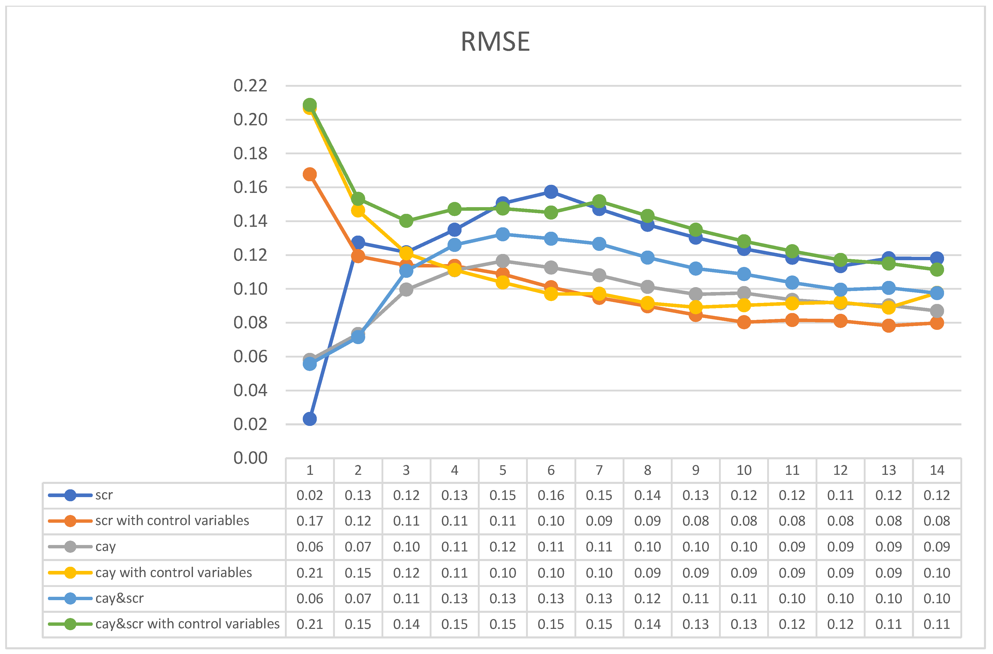
Regression 5 in Table 10 indicates the outcomes of RMSE that indicate that scrtcayt can forecast short-term horizon returns precisely. The RMSE increases from the second quarter to the sixth, indicating that it is not a good means of forecasting in the mid-term horizon. For the long-term horizon, from the 7th to the 14th quarters, it decreases (from 0.12664 to 0.097531), which indicates better performance than that for the mid-term horizon. At regression 6, including two-state variables with control variables, the orientation of the series decreases from the 1st to the 14th step. In the short term and mid-term, its values are high, which is not proper. In the long run, it has better performance. Its TIC approach is similar to its RMSE. Compared to previous regressions, regressions 5 and 6 cannot provide a more definite prediction. So, Hypothesis 3 has been rejected. By comparing the RMSE amounts of different regressions, as shown in Figure 5, over the short-term, scrt is the best at forecasting. After the first quarter, to the long-term horizon, the best prediction is achieved by regression 3 (cayt). Figure 6 shows the RMSE trend of the regressions with control variables. scrt with control variables is the best at forecasting in the short-term and long-term horizons. Of course, the difference compared to cayt with control variables is small. In the mid-term background, from 4th to the 6th quarter, cayt has better performance. Following this, a general figure summarizing all regression performances is provided in Figure 7.

4.4. Further Diagnostic Test: The Jarque–Bera Statitics

A post-estimation diagnostic test was conducted to assess model adequacy. According to the p-values (as shown in Table 11), the Jarque–Bera normality test on residuals [42] fails to reject normality. So, this confirms that regression residuals are approximately normally distributed. The detailed components are reported in Tables S9–S11.

4.5. Regression Test Based on Nonlinear TSLS Estimation

We use the variance ratio to analyze the state variables’ illustrative potential. In Equation (11), the regression variables on the right side are orthogonalized. As a result, we can compute the variance decomposition of the required excess returns as follows:
V a r E t t = 1 k r i , t + k e = V a r ( a k z t ) + V a r ( β 1 k s c r t ) + V a r ( β 2 k c a y t )
Equation (11) declares that the share of the variation in expected K-period excess returns, that can be described by scr and cay, can be calculated, respectively, by the following variance ratios:
0 V R s c r k = V a r ( β 1 k s c r t ) V a r ( a k z t ) + V a r ( β 1 k s c r t ) + V a r ( β 2 k c a y t ) 1
0 V R c a y k = V a r ( β 2 k c a y t ) V a r ( a k z t ) + V a r ( β 1 k s c r t ) + V a r ( β 2 k c a y t ) 1
We assessed the entire amount of predictable variance in excess returns that can be accounted for by scrt and cayt using Nonlinear Two Stage Least Squares (N-TSLS). We are unable to use the OLS approach as the variance ratio equation is nonlinear. In a nonlinear regression technique, the model with endogenous explanatory variables is examined using N-TSLS. A variable that has a correlation with the regression model’s error term is called an endogenous variable. Using an endogenous variable goes against OLS’s presumptions. The fundamental idea behind the TSLS technique is to forecast the model’s elements using instrumental variables that are uncorrelated with the error term. The instrumental factors have no correlation with the model’s error term, in contrast to the endogenous variables. The N-TSLS estimate findings for the explanatory power of scr and cay are shown in Table 12.
The coefficient of scr (β1) is significantly negative. This means that its relationship with the expected return is indirect. The coefficient of cay (β2) is significantly positive. This implies that the relationship of cayt with the expected return is direct. Regarding the RMSE, our findings show that the RMSE of scrt (Regression 12) at short horizons has the best performance with the lowest value (0.006). This is matches with the theory. After that, in 2nd quarter, it increases up to 0.019. And then it decreases from 0.017 (3th quarter) to 0.014 (5th quarter). After that, it is almost constant (about 0.014) from the 6th quarter to the 10th quarter. Next, it increases from 0.015 (11th quarter) up to 0.016 (12th quarter). And forwards it decreases (13th quarter). And finally, it increases again (14th quarter). The TIC approach is similar. Regression 12 further validates Hypothesis 1.
In cayt, the best performance occurred in the first step (0.007). From the second to the third quarter, the RMSE increases from 0.012 to 0.013. And then from the forth quarter to fifth quarter the RMSE decreases from 0.011 to 0.010. Next it increases again from 0.012 (6th quarter) up to 0.028 (12th quarter). This increase in RMSE shows this regression is not so dominant in mid-term forecasting. Finally, it decreases from 0.020 (13th quarter) to 0.014 (14th quarter). This shows that forecasting using this regression is more suitable in the long-term than it is in the mid-term horizon. The TIC approach is similar to RMSE, which is in line with Hypothesis II. The next table (Table 13) shows the results of N-TSLS and OLS simultaneously.
To analyze Table 12, we categorized all quarters into three main categories. The first is the short term. For N-TSLS regression, the RMSE of scrt in the first quarter (short-term) is less than cayt (0.006 vs. 0.0076). It is similar to OLS regression, such that the result of scrt is more reliable that that of cayt (0.023 vs. 0.0581). Secondly, in the mid-term, the trend of fluctuations of N-TSLS in comparison to OLS is slightly different, and N-TSLS is less reliable. Last but not least, in the long term, cayt results have less error than scrt in the long-term horizon (0.0144 vs. 0.0167). This is also similar to OLS regression (0.0799 vs. 0.087). In general, the results obtained from the robustness test verify the results of the research and show that they are significant.

5. Conclusions

The primary obstacle that relevant academics and investors face is estimating stock returns using asset price parameters. Thus, this research aims to tackle this difficulty by using actual stock data. Given the high degree of integration between the Chinese stock market and the world market, this research used China as a case study to investigate the predictive capacity of the consumption-based Capital Asset Pricing Model (CAPM) for stock returns. Campbell and Cochrane’s habit formation model predicts time varying returns. According to this model, scrt-based return predictability is implied. In addition, cayt is used in the main stock market return expectation assessments. Logarithmic consumption (ct), logarithmic asset holding (at), and logarithmic labor income (yt) are all part of the same technique that yields cayt. Our research reveals a link between log consumption, log asset ownership, and log labor income via cointegration.
In this research, we apply the consumption-based CAPM via two-state variables such as scrt and cayt. These state variables are considered separately and together as different regressors. Using control variables (including dividend yield, dividend payout ratio, and government bond term spread) can improve the estimation results. Then, these state variables and control variables are formed into six regressions. We used the OLS procedure to test the forecast of stock market returns at the Shanghai Stock Exchange (SSE) with the above-mentioned regressors from 2012Q1 to 2018Q4. The coefficient correlation of scrt is negative, which means its relationship with the expected returns is inverse, and Hypothesis 1 is established. The confidence levels of scrt and cayt with the control variables’ prediction power are 90% and 95%, respectively. When the business cycle troughs, surplus consumption and investor risk aversion are high, while the expected or desired return is low. The coefficient correlation of cayt is positive, which means its relationship with the expected return is direct, and Hypothesis 2 is established. The confidence levels in the prediction power of cay and cay with control variables are both 99%, respectively. When investors expect more moderate returns on an asset in the coming days, they will decrease consumption in the present, accordingly, to below the long-term horizon connection of consumption, assets, and wealth, to ensure further consumption. For state variables considering the control variable, we find that scrt at short horizons has the best performance with the lowest RMSE value and predicts excess stock returns for extremely short timeframes. In spite of this, cayt has better forecasting performance than scrt for the mid-term and long-term horizons. The trend of estimation results using scrtcayt is the same as cayt, and, of course, its difference compared with cayt is small. In the regressions, including state variables with control variables, scrt with control variables is better at forecasting in the short-term horizon as well as the long-term horizon than cayt with control variables and scrtcayt with control variables. Generally, among all regressors, scrt in the short term, cayt in the medium term, and scrt with control variables in the long term are the optimal regressors. These results show that combining scrt and cayt did not improve the prediction power. Therefore, we reject Hypothesis 3. Finally, we tested the robustness of the proposed model using N-2SLS. The results of the robustness check show that our model has significant power. Our research contributes new knowledge to the forecasting of changes to the aggregate stock market returns in the Chinese stock market, and can be considered by investigators and researchers. Future research may extend the time period of the used data to evaluate other policy regimes. Also, the Shenzhen Stock Exchange could be considered to conduct a further analysis of the Chinese stock market.

Supplementary Materials

The following supporting information can be downloaded at: https://www.mdpi.com/article/10.3390/systems13121066/s1, Table S1: Household wealth, Table S2: Household disposable income, Table S3: Nondurable consumption, Table S4: Johansen, Table S5: Philips-Ouliaris Cointegration Test, Table S6: scrt, Table S7: cayt, Table S8: cayt and scrt, Table S9: scr normality test, Table S10: cay normality test, and Table S11: Double variables normality test.

Author Contributions

Conceptualization, F.Z.B.A.; Software, A.H.; Validation, A.H. and W.L.; Investigation, W.L.; Writing—original draft, F.Z.B.A.; Writing—review & editing, A.H. and W.L.; Supervision, W.L. All authors have read and agreed to the published version of the manuscript.

Funding

This research received no external funding.

Data Availability Statement

Data is contained within the article or Supplementary Material.

Conflicts of Interest

The authors declare no conflict of interest.

References

  1. Sun, G.; Li, Y. Intraday and Post-Market Investor Sentiment for Stock Price Prediction: A Deep Learning Framework with Explainability and Quantitative Trading Strategy. Systems 2025, 13, 390. [Google Scholar] [CrossRef]
  2. Zhang, X.; Yang, X.; He, Q. Multi-Scale Systemic Risk and Spillover Networks of Commodity Markets in the Bullish and Bearish Regimes. N. Am. J. Econ. Financ. 2022, 62, 101766. [Google Scholar] [CrossRef]
  3. Wang, Y.; Gu, W.; Ma, B.; Sun, G.; Kang, X. Does the opening of the China’s stock market improve market liquidity? Financ. Res. Lett. 2025, 85, 108273. [Google Scholar] [CrossRef]
  4. Liu, Y.; Zhang, L.; Failler, P.; Wang, Z. The Dynamic Evolution of Agricultural Trade Network Structures and Its Influencing Factors: Evidence from Global Soybean Trade. Systems 2025, 13, 279. [Google Scholar] [CrossRef]
  5. Lyu, J.; Li, Z. Time-Varying Spillover Effects of Carbon Prices on China’s Financial Risks. Systems 2024, 12, 534. [Google Scholar] [CrossRef]
  6. Fehrle, D.; Heiberger, C. The return on everything and the business cycle in production economies. Econ. Model. 2024, 136, 106742. [Google Scholar] [CrossRef]
  7. Kwan, Y.K.; Leung, C.K.Y.; Dong, J. Comparing Consumption-Based Asset Pricing Models: The Case of an Asian City. J. Hous. Econ. 2015, 28, 18–41. [Google Scholar] [CrossRef]
  8. Polimenis, V. The historical lepto-variance of the US stock returns. Data Sci. Financ. Econ. 2024, 4, 270–284. [Google Scholar] [CrossRef]
  9. French, J. A Practitioner’s Guide to the CAPM: An Empirical Study. In Global Tensions in Financial Markets; Research in Finance; Emerald Publishing Limited: Leeds, UK, 2018; Volume 34, p. 1. [Google Scholar]
  10. Vendrame, V.; Guermat, C.; Tucker, J. A Conditional Regime Switching CAPM. Int. Rev. Financ. Anal. 2018, 56, 1–11. [Google Scholar] [CrossRef]
  11. Engsted, T.; Hyde, S.; Møller, S. V Habit Formation, Surplus Consumption and Return Predictability: International Evidence. J. Int. Money Financ. 2010, 29, 1237–1255. [Google Scholar] [CrossRef]
  12. Boudoukh, J.; Michaely, R.; Richardson, M.; Roberts, M.R. On the Importance of Measuring Payout Yield: Implications for Empirical Asset Pricing. J. Financ. 2007, 62, 877–915. [Google Scholar] [CrossRef]
  13. McMillan, D.G. Consumption and Stock Prices: Evidence from a Small International Panel. J. Macroecon. 2013, 36, 76–88. [Google Scholar] [CrossRef]
  14. John, Y.C.; Shiller, R.J. Valuation Ratios and the Long-Run Stock Market Outlook. J. Portf. Manag. 1998, 24, 11–26. [Google Scholar] [CrossRef]
  15. Xiao, Y.; Faff, R.; Gharghori, P.; Min, B.K. Pricing Innovations in Consumption Growth: A Re-Evaluation of the Recursive Utility Model. J. Bank. Financ. 2013, 37, 4465–4475. [Google Scholar] [CrossRef]
  16. Liu, L.; Wang, Z. A Note on an Interpretation to Consumption-Based CAPM. Econ. Lett. 2008, 99, 443–445. [Google Scholar] [CrossRef]
  17. Chang, T.; Gupta, R.; Majumdar, A.; Pierdzioch, C. Predicting Stock Market Movements with a Time-Varying Consumption-Aggregate Wealth Ratio. Int. Rev. Econ. Financ. 2019, 59, 458–467. [Google Scholar] [CrossRef]
  18. Lettau, M.; Ludvigson, S. Resurrecting the (C)CAPM: A Cross-Sectional Test When Risk Premia Are Time-Varying. J. Polit. Econ. 2001, 109, 1238–1287. [Google Scholar] [CrossRef]
  19. Balcilar, M.; Bekiros, S.; Gupta, R. The Role of News-Based Uncertainty Indices in Predicting Oil Markets: A Hybrid Nonparametric Quantile Causality Method. Empir. Econ. 2017, 53, 879–889. [Google Scholar] [CrossRef]
  20. Fung, K.W.T.; Lau, C.K.M.; Chan, K.H. The Conditional Equity Premium, Cross-Sectional Returns and Stochastic Volatility. Econ. Model. 2014, 38, 316–327. [Google Scholar] [CrossRef]
  21. Márquez, E.; Nieto, B.; Rubio, G. Stock Returns with Consumption and Illiquidity Risks. Int. Rev. Econ. Financ. 2014, 29, 57–74. [Google Scholar] [CrossRef]
  22. Li, B.; Zhong, M. Predictability of Stock Returns and Consumption-Based CAPM: Evidence from a Small Open Market. Eur. J. Econ. Financ. Adm. Sci. 2010, 22, 148–173. [Google Scholar]
  23. Farag, H.; Meng, Q.; Mallin, C. The Social, Environmental and Ethical Performance of Chinese Companies: Evidence from the Shanghai Stock Exchange. Int. Rev. Financ. Anal. 2015, 42, 53–63. [Google Scholar] [CrossRef]
  24. Chen, C.; Hu, C.; Yao, H. Behavioral Framework of Asset Price Bubbles: Theoretical and Empirical Analyses. Systems 2022, 10, 251. [Google Scholar] [CrossRef]
  25. Guo, B.; Zhang, W.; Zhang, Y.; Zhang, H. The Five-Factor Asset Pricing Model Tests for the Chinese Stock Market. Pac.-Basin Financ. J. 2017, 43, 84–106. [Google Scholar] [CrossRef]
  26. Meng, Q.; Qi, J.; Wang, S.; Zhao, X. Disciplining the Factor Zoo: Identifying Pricing Factors in the Chinese Stock Market. Econ. Model. 2025, 155, 107370. [Google Scholar] [CrossRef]
  27. Zhang, Y.; Jia, Q.; Chen, C. Risk Attitude, Financial Literacy and Household Consumption: Evidence from Stock Market Crash in China. Econ. Model. 2021, 94, 995–1006. [Google Scholar] [CrossRef]
  28. Huang, T.-L. Is the Fama and French Five-Factor Model Robust in the Chinese Stock Market? Asia Pac. Manag. Rev. 2019, 24, 278–289. [Google Scholar] [CrossRef]
  29. Chen, C.-D.; Demirer, R.; Jategaonkar, S.P. Risk and Return in the Chinese Stock Market: Does Equity Return Dispersion Proxy Risk? Pac.-Basin Financ. J. 2015, 33, 23–37. [Google Scholar] [CrossRef]
  30. Le, A.T.; Nguyen, H.; Nguyen, C. Regret to reward: Investor regret and the cross-sectional stock returns in the Chinese market. Glob. Financ. J. 2025, 68, 101205. [Google Scholar] [CrossRef]
  31. Kang, J.; Kim, T.S.; Lee, C.; Min, B.-K. Macroeconomic Risk and the Cross-Section of Stock Returns. J. Bank. Financ. 2011, 35, 3158–3173. [Google Scholar] [CrossRef]
  32. Itoy, M.; Noda, A. CCAPM with Time-Varying Parameters: Some Evidence from Japan; Keio Economic Society, Keio University: Tokyo, Japan, 2011. [Google Scholar]
  33. Liu, L.; Wan, J. The Relationships between Shanghai Stock Market and CNY/USD Exchange Rate: New Evidence Based on Cross-Correlation Analysis, Structural Cointegration and Nonlinear Causality Test. Phys. A Stat. Mech. Its Appl. 2012, 391, 6051–6059. [Google Scholar] [CrossRef]
  34. Koutmos, D.; Song, W. Speculative Dynamics and Price Behavior in the Shanghai Stock Exchange. Res. Int. Bus. Financ. 2014, 31, 74–86. [Google Scholar] [CrossRef]
  35. Auer, B.R. Can Habit Formation under Complete Market Integration Explain the Cross-Section of International Equity Risk Premia? Rev. Financ. Econ. 2013, 22, 61–67. [Google Scholar] [CrossRef]
  36. Li, Y. The Wealth-Consumption Ratio and the Consumption-Habit Ratio. J. Bus. Econ. Stat. 2014, 23, 226–241. [Google Scholar] [CrossRef]
  37. Møller, S.V. Habit Persistence: Explaining Cross-Sectional Variation in Returns and Time-Varying Expected Returns. J. Empir. Financ. 2009, 16, 525–536. [Google Scholar] [CrossRef]
  38. Bianchi, F.; Lettau, M.; Ludvigson, S.C. Monetary Policy and Asset Valuation; No. 22572; National Bureau of Economic Research: Cambridge, MA, USA, 2016. [Google Scholar]
  39. Caporale, G.M.; Sousa, R.M. Consumption, Wealth, Stock and Housing Returns: Evidence from Emerging Markets. Res. Int. Bus. Financ. 2016, 36, 562–578. [Google Scholar] [CrossRef]
  40. Gardberg, M.; Pozzi, L. Aggregate consumption and wealth in the long run: The impact of financial liberalization. J. Appl. Econom. 2022, 37, 161–186. [Google Scholar] [CrossRef]
  41. Xie, H. Nonlinear and nonseparable structural functions in regression discontinuity designs with a continuous treatment. J. Econom. 2024, 242, 105784. [Google Scholar] [CrossRef]
  42. Jarque, C.M.; Bera, A.K. Efficient tests for normality, homoscedasticity and serial independence of regression residuals. Econ. Lett. 1980, 6, 255–259. [Google Scholar] [CrossRef]
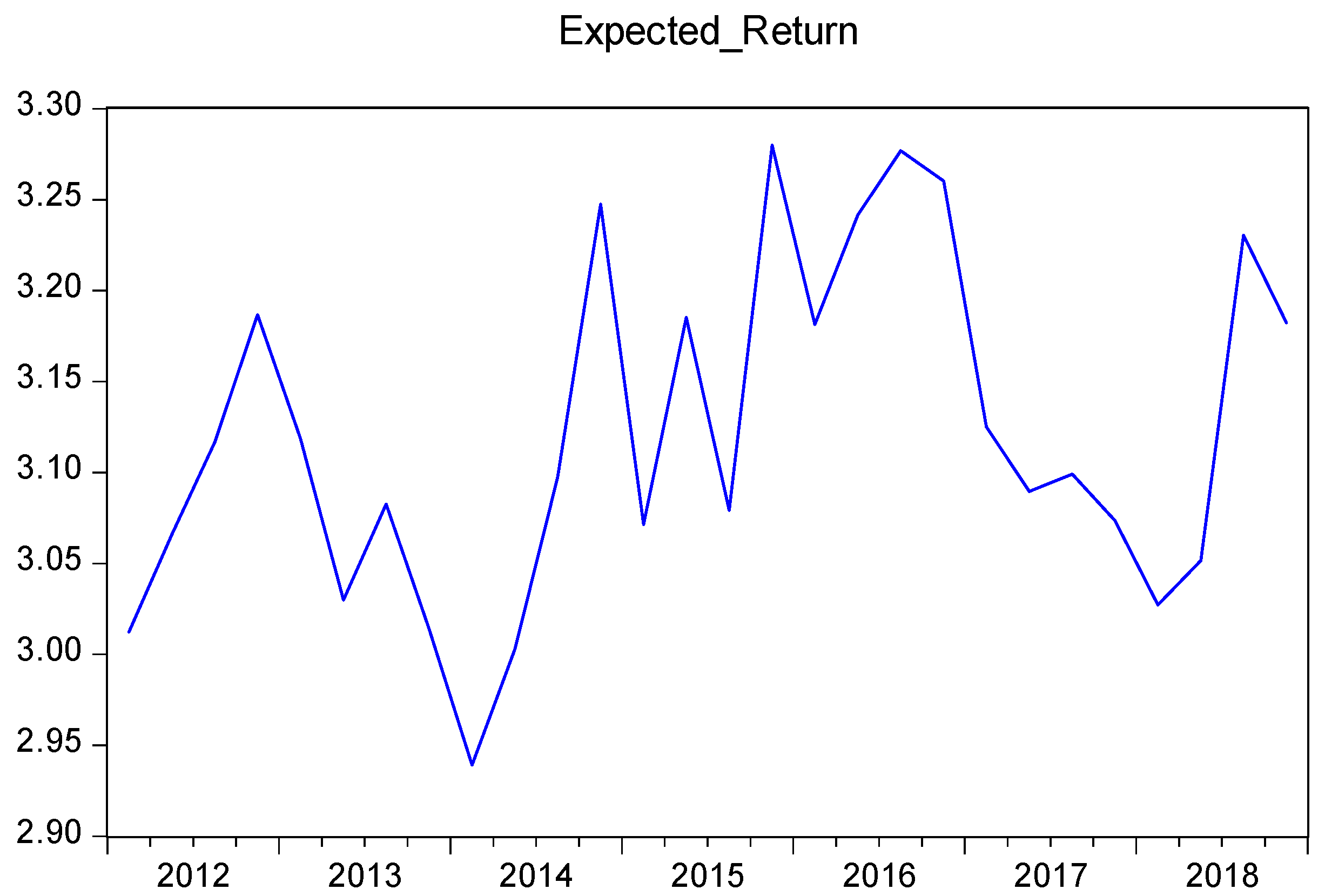
Figure 1. Expected return.
Systems 13 01066 g001
Figure 2. RMSE of return forecasting using scr and scr with control variables.
Systems 13 01066 g002
Figure 3. RMSE of return forecasting using cay and cay with control variables.
Systems 13 01066 g003
Figure 4. RMSE of return forecasting using two-state variables with control variables.
Systems 13 01066 g004
Figure 5. RMSE of return forecasting using scr and/or cay.
Systems 13 01066 g005
Figure 6. RMSE of return forecasting using scr and/or cay with control variables.
Systems 13 01066 g006
Figure 7. RMSE of return forecasting using all regressions.
Systems 13 01066 g007
Table 1. Some CCAPM studies on the Chinese stock market and the stock markets of some other countries.
Author(s)Method(s)Feature(s) and ResultsCase StudySource
Kang et al., (2011)Conditional CAPM using macroeconomic indices.- The conditioning variable had a durable power to predict market excess returns.
- The suggested variable strongly forecasts excess stock returns.
Korea[31]
Itoy and Noda (2011)Standard CCAPM- Using the Hansen method for generalized empirical likelihood (GEL) estimation.
- That both factors predicted the CCAPM, the degree of risk aversion, and the rate of time discount change over time.
Japan[32]
Liu and Wan (2012)Linear and nonlinear Granger causality tests- Examined the co-movement of the Shanghai stock market and exchange rates of Chinese currency (CNY).
- The stock price and exchange rate are significantly cross-correlated.
Shanghai Stock Exchange[33]
Koutmosa and Songb (2014)A range-based autoregressive volatility framework.- Examined the degree to which changes in asset portfolio stock prices reflect the trading patterns of diverse individuals.
- Information-driven investors believe that periods of declining stock prices are entirely tied to low-volume trading time, whereas rising stock prices are often associated with a significant quantity of trading time.
Shanghai Stock Exchange[34]
Vendrame, Guermat, and Tucker (2018)Conditional CAPM- There are severe time deviations in betas across their approaches and frameworks.
- The regime-switching framework deducts the proper prediction of one-day-ahead value-at-risk.
USA, Germany, England, France, China, and Malaysia[10]
Table 2. The details of the considered control variables.
NameSymbolCalculationDescription
Dividend yielddptThis is the coefficient of a corporation’s yearly dividend compared to its share price.A stock investment’s dividend-only return is predicted by the dividend yield. The yield will increase when the stock price declines and fall when the stock price rises, assuming that the dividend is neither increased nor decreased.
Dividend payout ratiodetThis is the overall volume ratio of dividends distributed to investors as a percentage of the firm’s net income.An innovative, growing company with ambitious intentions to expand into new markets and provide innovative results might be excused for its low payout ratio as it is anticipated to reinvest most or all of its profits.
Government bond term spreadTRMtThe China Bond Pricing Center provides this information as the difference between the China Bond Long Term Index and the China Bond Short-Middle Term Index.It is a crucial factor that bond funders calculate when gauging the level of const for single or plural bonds.
Table 3. Descriptive statistics of the considered factors.
IndicatorsMeanMedianMaximumMinimumStandard ErrorAutocorrelation
r3.120273.098233.279792.939120.017530.452
scrt−0.58781−0.59034−0.50139−0.695050.010390.871
cayt14.8636115.0479916.5627212.869880.210268−0.025
dpt6.631066.560137.460836.233850.056420.797
det6.0094585.974817.035745.533350.067950.790
TRMt6.095905.8056422.38690−10.668301.677780.848
Table 4. Summary of Correlation Matrix Statistics.
RscrtcaytdptdetTRMt
r1
scrt−0.257581
cayt0.503180.218551
dpt0.287460.228220.126731
det0.297780.242360.108290.994971
TRMt0.735010.654810.268170.380580.397791
Table 5. Return estimation using scrt/with control variables.
Variable(1)(2)
C2.991591 ***
(3.983746)
2.443527
(1.166974)
scrt−0.146233 *
(−0.120682)
−0.728282 **
(−0.988364)
det −0.162131
(−0.173376)
dpt 0.175458
(0.157883)
TRMt 0.014413 ***
(3.432777)
MA(1)0.385215
(1.011465)
−0.596789
(−3.58 × 10⁵)
MA(2)0.230451
(0.417315)
−0.403211
(−2.31 × 10⁵)
Observation1414
R-squared0.1204460.725737
Adjusted R-squared−0.2704660.405764
F-statistic0.3081152.268120
Note: the figures in parentheses are t-test values; ***, **, and * denote statistical significance at the 0.01, 0.05, and 0.10 level, respectively.
Table 6. Single State Variable Forecasting Regressions of scrt/with control variables.
Horizon12
RMSETICRMSETIC
Q10.023192-0.167689-
Q20.1273440.0202690.1193030.018486
Q30.1216660.0193950.1138670.017633
Q40.1349360.0214740.1135680.017493
Q50.1505750.023910.1087310.016671
Q60.157350.024960.100980.0155
Q70.147210.023410.094740.01461
Q80.137880.0219830.0897680.013916
Q90.1303080.0208120.0846340.013176
Q100.1236250.0197820.0803490.01256
Q110.1184420.0189950.08160.0128
Q120.1134650.0182250.0811160.012757
Q130.118080.018950.078270.0123
Q140.117960.018930.079920.01254
Table 7. Return estimation using cay/with control variables.
Variable(3)(4)
C2.435656 ***
(11.66133)
−0.079700
(−0.071793)
cayt0.045176 **
(3.211853)
0.042841 ***
(4.550892)
dpt 1.270126 *
(2.191582)
det −0.977815 *
(−2.055565)
TRMt 0.005716
(0.654912)
MA (1)0.591084
(1.578985)
0.391322
(0.000243)
MA (2)0.694545
(1.664657)
0.999991
(0.000121)
Observations1414
R-squared0.6005200.878058
Adjusted R-squared0.4229730.735793
F-statistic3.3823166.171977
Note: the figures in parentheses are t-test values; ***, **, and * denote statistical significance at the 0.01, 0.05, and 0.10 level, respectively.
Table 8. Single state variable forecasting regressions cayt/with control variables.
Horizon34
RMSETICRMSETIC
Q10.058083-0.206886-
Q20.0733980.0115650.1463290.022646
Q30.0995790.0157890.120990.018851
Q40.1110520.0175830.111220.017335
Q50.116510.0183870.1038090.016143
Q60.112610.017730.0970.01507
Q70.107990.017070.097180.01519
Q80.1012330.016040.0916310.014375
Q90.0968310.015360.0891940.014019
Q100.097560.0154880.0903270.014223
Q110.093510.014890.0914580.01444
Q120.0914980.0145910.0921580.014576
Q130.09030.014380.088950.01404
Q140.087020.013840.097660.01538
Table 9. Return estimation using scrt-cayt/with control variables.
Variable(5)(6)
C2.237905 ***
(3.298284)
−0.755299
(−0.606806)
Scrt−0.329407 *
(−0.359154)
−0.740563 *
−(0.708127)
Cayt0.044544 **
(2.789661)
0.036815 **
(3.026916)
det −0.981177
(−1.620132)
dpt 1.317897
(1.844020)
TRMt 0.004287 *
(0.606492)
MA(1)0.826218
(0.026679)
0.813163
(0.000236)
MA(2)0.997404
(0.013390)
1.000000
(0.000118)
Observation1414
R-squared0.6774450.897542
Adjusted R-squared0.4758470.733610
F-statistic3.3603885.475089
Note: the figures in parentheses are t-test values; ***, **, and * denote statistical significance at the 0.01, 0.05, and 0.10 level, respectively.
Table 10. Two-state variable forecasting regressions with control variables.
Horizon56
RMSETICRMSETIC
Q10.05567-0.208636-
Q20.0715380.0112720.1532570.023814
Q30.1106820.0175730.1402030.021989
Q40.1260130.019990.1471730.023134
Q50.1323020.0209240.1474830.023151
Q60.1296880.0204660.145140.022772
Q70.126640.0200720.1517850.023977
Q80.1185370.018840.143140.022701
Q90.1120.0178230.1349580.021445
Q100.1087540.0173230.1281630.020406
Q110.103720.0165760.122250.019524
Q120.0995310.0159340.1171020.018744
Q130.1006260.0160890.1149830.018376
Q140.0975310.0155820.1113980.017772
Table 11. The normality test (Jarque–Bera statistics).
Variable(s)ObservationsR-SquaredAdjusted R-SquaredF-StatisticJarque–Bera Test (p-Value)Output
cay280.60780.53968.910.3237Normality not rejected
scr280.60790.53978.920.3043Normality not rejected
scr-cay280.60820.51926.830.3231Normality not rejected
Table 12. Single state variable scr and cay forecasting regressions by N-TSLS.
Horizon78
RMSETICRMSETIC
Q10.006022-0.007581-
Q20.019960.0242540.0129140.022591
Q30.0177610.0226960.0136280.025247
Q40.0162890.0212910.0118970.02218
Q50.0149010.019560.0109430.020166
Q60.0143350.019040.0123880.022193
Q70.0146960.019890.017590.03198
Q80.0147890.0202670.0214220.038759
Q90.0145480.0200490.0225920.040363
Q100.0145530.0202040.0239350.041983
Q110.0152920.021530.0258490.045739
Q120.0160080.0228350.0288460.050818
Q130.0151850.7616890.020870.041536
Q140.0167230.0242810.014390.032061
Moment ConditionsOrthogonal to
u 1 t k = k = 1 K r t + k e ( a 0 k + a k z t + β 1 k s c r t + β 2 k c a y t ) 1 , z ( 1 ) , s c r t , c a y t
u 2 t = [ ( a k z t ) 2 + ( β 1 k s c r t ) 2 + ( β 2 c a y t ) 2 ]   V R s c r k ( β 1 k s c r t ) 2 1
u 3 t = [ ( a k z t ) 2 + ( β 1 k s c r t ) 2 + ( β 2 k c a y t ) 2 ]   V R c a y k ( β 2 k c a y t ) 2 1
Table 13. Comparison of RMSE in the proposed method and robustness method.
Horizoncayscr
N-TSLSOLSN-TSLSOLS
Q10.00760.05810.00600.0232
Q20.01290.07340.02000.1273
Q30.01360.09960.01780.1217
Q40.01190.11110.01630.1349
Q50.01090.11650.01490.1506
Q60.01240.11260.01430.1574
Q70.01760.10800.01470.1472
Q80.02140.10120.01480.1379
Q90.02260.09680.01450.1303
Q100.02390.09760.01460.1236
Q110.02580.09350.01530.1184
Q120.02880.09150.01600.1135
Q130.02090.09030.01520.1181
Q140.01440.07990.01670.0870
Disclaimer/Publisher’s Note: The statements, opinions and data contained in all publications are solely those of the individual author(s) and contributor(s) and not of MDPI and/or the editor(s). MDPI and/or the editor(s) disclaim responsibility for any injury to people or property resulting from any ideas, methods, instructions or products referred to in the content.