Article

Passenger Switch Behavior and Decision Mechanisms in Multimodal Public Transportation Systems

1
School of Transportation, Jiulonghu Campus, Southeast University, Nanjing 211100, China
2
Department of Cooperation and Exchange, Mianyang Normal University, Mianyang 621000, China
3
Transportation Institute, Inner Mongolia University, Huhehaote 010020, China
*
Author to whom correspondence should be addressed.
Systems 2025, 13(11), 951; https://doi.org/10.3390/systems13110951 (registering DOI)
Submission received: 24 September 2025 / Revised: 17 October 2025 / Accepted: 24 October 2025 / Published: 26 October 2025

Abstract

Efficient public transportation systems are fundamental to achieving sustainable urban development. As the backbone of urban mobility, the coordinated development of rail transit and bus systems is crucial. The opening of a new rail transit line inevitably reshapes urban travel patterns, posing significant challenges to the existing bus network. Understanding passenger switch behavior is key to optimizing the competition and cooperation between these two modes. However, existing methods on the switch behavior of bus passengers along the newly opened rail transit line cannot balance the predictive accuracy and model interpretability. To bridge this gap, we propose a CART (classification and regression tree) decision tree-based switch behavior model that incorporates both predictive and interpretive abilities. This paper uses the massive passenger swiping-card data before and after the opening of the rail transit to construct the switch dataset of bus passengers. Subsequently, a data-driven predictive model of passenger switch behavior was established based on a CART decision tree. The experimental findings demonstrate the superiority of the proposed method, with the CART model achieving an overall prediction accuracy of 85%, outperforming traditional logit and other machine learning benchmarks. Moreover, the analysis of factor significance reveals that ‘Transfer times needed after switch’ is the dominant feature (importance: 0.52), and the extracted decision rules provide clear insights into the decision-making mechanisms of bus passengers.

1. Introduction

With the acceleration of urbanization, the scale and population of the city are expanding, and traffic congestion, environmental pollution, and other problems are becoming more and more serious [1]. In order to solve these problems, a development framework focusing on ‘public transport priority’ came into being [2,3]. Owing to its large capacity, high speed, and reliability, rail transit is critical to public transportation systems and is often viewed as a primary solution to diverse urban traffic issues.
With more and more rail transit lines being constructed and in operation, the competition and cooperation between rail transit and existing bus lines have become an important issue worth studying. After making use of rail transit, the passengers of bus lines overlapping with rail transit may be attracted to the latter. The research carried out by Sun also indicates that most of the new metro passengers are not from private transport (cars), but from the existing bus transit [4]. Therefore, it is necessary to accurately predict the switch behavior of bus passengers. This can provide a valuable reference for bus-line adjustment and new rail transit line planning. At the same time, accurate analysis of the relevant factors that affect the passenger switch can also help to formulate more targeted public transport policies. Furthermore, understanding passenger switching behavior extends beyond operational efficiency; it is integral to achieving sustainable urban mobility [5]. Optimizing multi-modal integration enhances public transport’s service quality and attractiveness, which is a key objective in analytical studies under the soft-computing paradigm [6]. This optimization is increasingly crucial with the rise in micromobility options (e.g., e-scooters, e-bikes), which critically reshape last-mile connectivity and final decisions on mode of transport [7]. It implies that the switch behavior model should incorporate both predictive and interpretive abilities.
Due to the limitations on data collection, existing studies are developed with questionnaire data (RP, SP). The quantity and accuracy of data samples are usually difficult to guarantee [8]. For this reason, earlier studies describe the switch behavior with logit-based models. It is easier to implement and very efficient to train with a relatively small sample set [9], and the model coefficients can be interpreted as indicators of feature importance [10]. However, due to the strict mathematical assumptions, the prediction accuracy of these methods is generally low [11].
In recent years, machine learning methods with powerful predictability attract a lot of interest and are widely applied to behavioral modeling [12,13,14,15]. Empirical research shows that it outperforms logit-based methods in terms of predictive accuracy. However, the internal principles of most data-driven methods are black boxes and lack interpretability, making it difficult to describe the decision-making principles of passenger behavior in detail. In addition, data-driven methods based on deep learning rely on a large amount of labeling sample data, leading to high cost of data collection.
This study aims to model the passenger switch behavior by combining the advantages of the two aforementioned methods. Figure 1 presents a flowchart outlining the main steps of our approach. Specifically, using the before–after passenger swiping-card data, we construct the bus passengers’ switch dataset. Based on the bus passengers’ switch dataset, we extract 12 factors that may affect switch behavior. Using the extracted factors, we establish a bus passenger switch behavior model based on a CART (classification and regression tree) decision tree. Finally, according to the generated tree model, we explore the rules that dictate bus passengers’ switch decision-making behavior. Its contributions are two-fold.
(1) A CART decision tree is constructed for the passenger switch behavior model. It considers 12 factors (including 6 personal travel attribute features, 3 socio-economic features, and 3 switch process features) that may affect bus passengers’ switch behavior. The proposed method can accurately predict the switch behavior of bus passengers and provide deep insights into the decision-making mechanism of passengers.
(2) The generated CART decision tree model is evaluated with a field-test before–after dataset. The experiment results show that our method improves the predictive accuracy of switch behavior significantly. We also analyze the sensitivity of each influencing factor, and mine the decision rules of people’s switch decision-making behavior, which can allow us to better understand people’s transfer behavior. Such empirical experiments demonstrate that the proposed CART decision tree model can predict the switch behavior accurately without loss of interpretability.
The rest of the paper is organized as follows. Section 2 is a literature review. Section 3 defines the problem. Section 4 constructs the bus passengers’ switch dataset and builds the bus passengers’ switch behavior model based on the CART decision tree. Section 5 is the experiment research. Section 6 is the conclusions and recommendations.
To precisely guide the experimental validation and clarify the contributions of this work, we formulate the following two testable hypotheses:
H1: 
The CART decision tree model will achieve statistically superior prediction accuracy for passenger switch behavior compared to traditional logit models and other benchmark machine learning methods.
H2: 
The CART model will provide interpretable decision rules that reveal key factors influencing passenger switch behavior.

2. Literature Review

At present, some scholars have analyzed the competition and cooperation between bus and rail transit systems [16]. Regarding the problem of bus passengers switching after the opening of the new rail transit, we mainly review the literature from two aspects: data sources and method categories.
Currently, most research on passenger switching behavior is based on questionnaire data. An analysis of stated preference data by Anwar et al. [9] on modal shifts from car and taxi to rail transit identified travel time, cost, and walking time as significant negative influences on individuals’ choice. Ting [17] extracted gender, occupation, salary, travel purpose, travel cost, travel time, and other factors that affect passenger switch based on SP survey data. The results show that the sensitivity of travel costs to passengers’ willingness to switch is greater than travel time. Through RP survey data, Jiabin [18] analyzed the switch characteristics of passengers after the opening of Wuxi Rail Transit Line 1, emphatically analyzed the travel time and cost factors affecting the switch of passengers, and further studied the adjustment method of bus lines. Based on 150 RP survey samples, Liang et al. [19] analyzed the changes in travel time and costs for passengers after the opening of the Shanghai Rail Transit Line 6. The experimental results show that the main factors that determine whether passengers switch to the rail transit are travel time, transfer times after switch, and the travel cost, while gender and age have little influence. Using online survey data, Wang et al. [20] analyzed the travel mode choice behavior of commuters in Shanghai during peak hours. Harrington and Parolin [21] conducted a six-month follow-up survey on passenger travel in the two composite corridors of rail transit and bus lines in Sydney. It was found that there was a competition between bus and rail systems, but the passengers of these two modes are different in age, occupation, travel purpose, and travel distance. Based on this, the target passengers for the two modes of transportation were determined and a commercial operation strategy was proposed. Through a study, Denizli, Turkey, Murat, and Cakici [22] investigated user perceptions within the public transportation system. The analysis of bus and paratransit modes in the study revealed that fare is a significant determinant of public transportation demand. Based on the RP and SP survey data, Wang et al. [23] studied the switch from bus transit, taxis, bicycles and other transportation modes to rail transit after the opening of Xi’an Rail Transit Line 2. The study found that 66.7% of rail transit passengers switched from bus transit, and salary, travel time, and cost are several important factors affecting a passenger’s decision to switch. It can be seen from the above research that the data used by most scholars at present is questionnaire data. Due to their high cost, the quantity and quality of the questionnaire data samples is also difficult to guarantee. In addition, it is difficult to use questionnaire data to field test. On the contrary, passenger swiping-card data is extensive and reliable [24,25,26]. Klar and Rubensson [27] leveraged smart card data to examine the evolution of spatio-temporal demand for public transport in the Stockholm region between 2017 and 2020. Leveraging the extensive dataset from Chile’s Transantiago bus system, Ruiz et al. [28] analyzed the impact of waiting time, bus occupancy, and speed on passenger satisfaction, which ensured the robustness of their findings. So, this paper studies the bus transit passengers’ switch behavior based on the data from passenger swiping cards, and conducts field tests. In addition, based on the factors mentioned in previous studies such as travel time, travel cost, and transfer times after the switch, this paper extracts a total of 12 influencing factors that may affect passenger switch, including passenger travel habit features, switch process features, and socio-economic features based on passenger swiping-card data.
The passenger switch problem is broadly a travel behavior problem [29,30]. The study of travel behavior is mainly supported by model-based methods, among which the most important are the logit series (multinomial logit model, nested logit model, and mixed logit model) [31,32,33]. Ma et al. [34] studied the joint choice behavior of commuters on travel time and travel mode by using the nested logit model. Ting [17] established a passenger switch model based on logit for Xian Metro with an accuracy of 72%. Liang, Wu, and Wang [19] built the utility function and mode competition selection model for bus transit and rail transit based on logit. Logit models have high interpretability based on probability-based statistical principles, but due to the strict mathematical assumptions, the prediction accuracy of these methods is always low.
Recently, the data-driven method has become more and more popular in the behavior modeling fields [35]. Some empirical studies show that machine learning outperforms logit models in prediction ability [36]. Mane et al. [37] used the binary logistic method and the Artificial Neural Network method (ANN) to establish models to evaluate the impact of BRT service on mode switch after private vehicles were introduced into BRT lanes. The experimental results show that ANN provides more accurate results than the binary logit model (BLM). Pineda-Jaramillo and Arbeláez-Arenas [38] conducted a comparative analysis of various logit models against machine learning algorithms, including Gradient Boosting and Random Forest. Their results demonstrated that an optimized Gradient Boosting model significantly outperformed all logit-based counterparts in predicting travel mode choice among public transport, private transport, and walking in an urban context. In their study of a light rail transit system in Izmir, Turkey, Özuysal et al. [39] employed both multiple regression and ANN models to estimate passenger flow. The evaluation showed that the ANN model yielded significantly better performance, especially for estimating flows at less busy stations. Ashik et al. [40] applied machine learning models to investigate the impact of the built environment on commuting mode choice in a high-density megacity context. Their empirical findings from Dhaka, Bangladesh, demonstrated that the built environment carried greater weight than socio-demographic factors in influencing commuting behavior. A comparative analysis of multinomial logit (MNL), Support Vector Machine (SVM), and Artificial Neural Network (ANN) models for travel mode choice was conducted by Zhang and Xie [36] using San Francisco data. Their evaluation concluded that the SVM framework yielded superior predictive accuracy. Beyond the classical machine learning models discussed, the field is rapidly advancing with the application of more sophisticated soft-computing techniques. These include fuzzy decision systems, which are adept at handling the inherent imprecision and subjectivity in passenger perceptions of service quality [6]. Hybrid models, which integrate the strengths of different algorithms (e.g., combining optimization techniques with machine learning), and ensemble learning methods (e.g., Gradient Boosting, Random Forest) have demonstrated a remarkable capacity to capture complex, non-linear relationships in travel behavior, often achieving state-of-the-art predictive performance [41,42]. Although the above models have achieved good prediction accuracy, the interpretability of the model is poor; for passenger behavior analysis, the interpretability of the model is also very important.
The tension between high predictive accuracy and model interpretability has catalyzed the rise in Explainable AI (XAI) as a critical research frontier, including in transportation science. Recent studies have increasingly emphasized the need for models that are not only accurate but also transparent and trustworthy for decision support in public policy and planning [43,44]. Within the XAI paradigm, models can be categorized as either post hoc (applying explanation techniques after a complex model has made a prediction) or intrinsically interpretable (using models that are understandable by their very design, such as decision trees and linear models) [45]. While powerful post hoc methods exist for explaining complex models, there is a strong argument for prioritizing intrinsically interpretable models when the goal is to gain direct insight into the decision-making process itself [46,47].
Classification and regression tree (CART) is also a machine learning algorithm. Because of the tree data structure, the CART decision tree has high prediction accuracy and good model interpretability. The tree operates by splitting the feature space at its nodes based on binary rules, progressing recursively until the leaf nodes are reached, which assign the final class labels [48]. Decision trees offer the advantage of being inherently interpretable while also effectively modeling nonlinearities and variable interactions [49]. Xie et al. [50] compared classification tree (CT) and ANN with MNL model. They concluded that CT and ANN perform better than MNL. In addition, they point out that CT is more effective and provides a better interpretation than ANN. However, at present, there is no research on the application of decision tree to the prediction of bus transit passengers’ decision to switch after the opening of rail transit. In this context, the CART (classification and regression tree) algorithm used in this study is a quintessential example of an intrinsically interpretable model. This paper proposes a bus passengers’ switch behavior model based on the CART decision tree and passenger swiping-card data. Its selection is a direct response to the call for transparency in XAI. The tree structure naturally reveals the hierarchy and thresholds of influencing factors, and the extracted IF-THEN rules provide causal, auditable logic for passenger switch behavior. This paper can mine passengers’ switch decision-making rules according to the generated tree model, which can better understand people’s switch behavior. This approach aligns with the core XAI principle of enabling human understanding and fostering trust in AI-driven insights, which is paramount for their adoption in real-world transport planning and policy-making. To systematically contextualize the methodological landscape and the contribution of this study, a comparative analysis of representative approaches is summarized in Table 1.

3. Related Definitions

Given the shared corridor between the new rail line and existing bus lines (Figure 2), a portion of bus passengers are likely to shift to rail transit upon its opening to complete their journeys. For a bus travel OD (the origination and the destination of the travel) of a passenger in a certain time period before the opening of the rail transit, if the passenger has completed this OD in the same time period with the help of the rail transit after the opening of the rail transit (including completion only by ‘Rail transit’ or ‘Rail transit + Bus’ or ‘Bus + Rail transit’ or ‘Bus + Rail transit + Bus’), then it is assumed that the passenger has switched to the metro under this OD in this time period. As shown in Figure 2, for the passengers whose original bus travel OD is in the AA and CC sections, they will theoretically not have switched. Therefore, our research target is the passengers whose original bus travel OD is in the BB, AB, BC, and AC sections. For the passengers whose original bus travel OD is in section BB, they will take rail transit to complete the switch (only rail transit); for the passengers in section AB, they will take a bus first, then transfer to the rail transit and take rail transit to complete the switch (Bus + Rail); for the passengers in section BC, they will take rail transit first, then transfer to the bus and take a bus to complete the switch (Rail + Bus); for the passengers in section AC, they will take a bus first, then transfer to the rail transit and take rail transit, then transfer to the bus and take a bus to complete the switch (Bus + Rail + Bus).

4. Materials and Methods

4.1. Bus Passengers’ Switch Dataset Construction Based on Passenger Swiping-Card Data

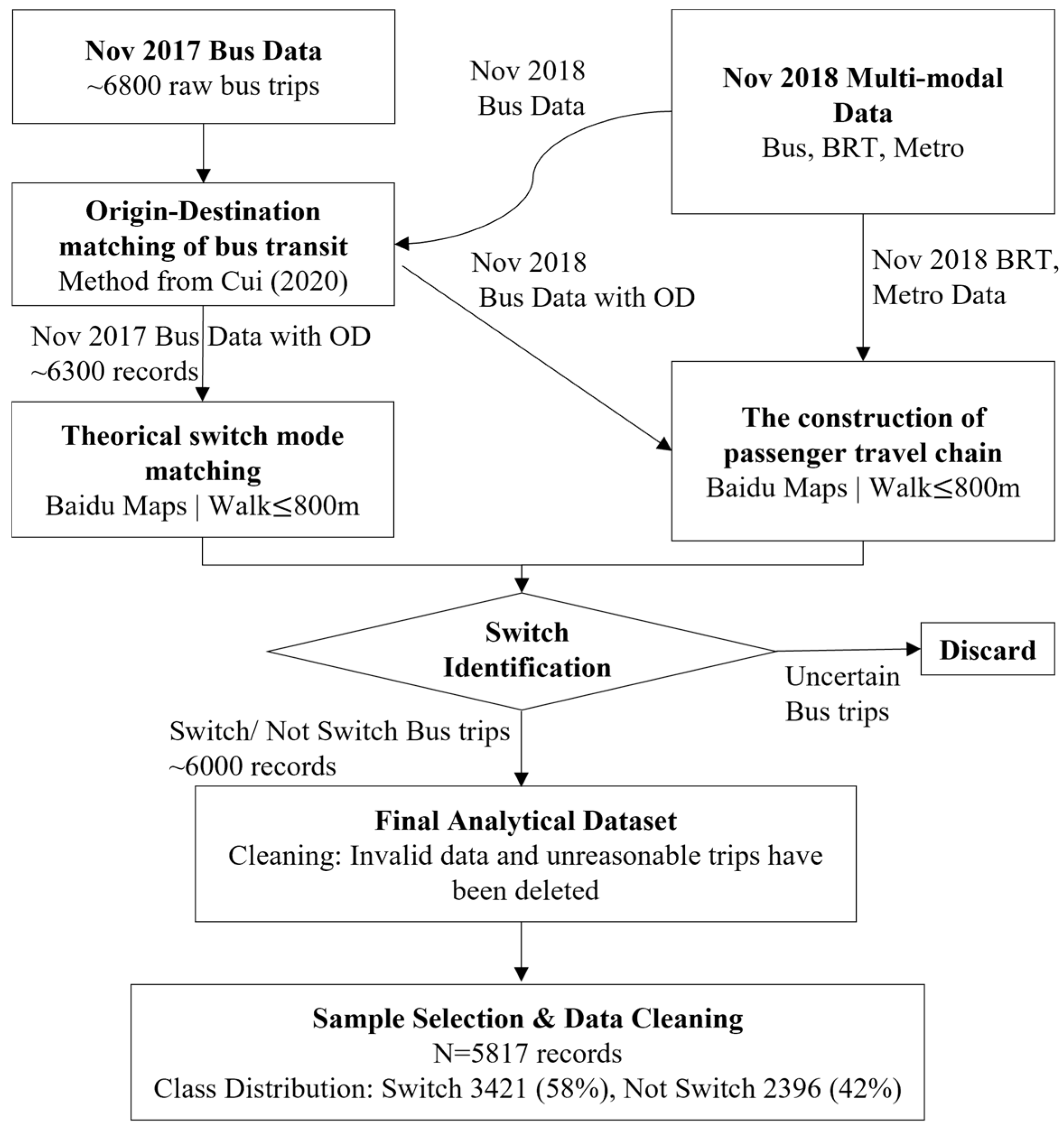
In Xiamen, the ‘Yitong card’ (a kind of intelligent card) is in common use for all public transportation payment systems. People can use the ‘Yitong card’ to take the bus, BRT, and rail transit. Therefore, this paper can identify the passenger’s switch behavior after the opening of the rail transit according to the ‘Yitong card’ data. The identification process is shown in Figure 3. Since Xiamen Rail Transit Line 1 started operating on 1 January 2018, this paper used the ‘Yitong card’ data of passengers in November 2017 and November 2018 for research. Next, we will refer to Figure 3 to explain the process of passenger switch behavior recognition.

4.1.1. Origin–Destination Matching of Bus Transit

Due to the one-ticket charging system adopted by Xiamen’s bus transit system, passengers swipe their cards when getting on the bus but do not swipe when getting off. Hence, the passenger’s boarding stop is directly available, but the alighting stop must be inferred. This paper employs an enhanced alighting-stop determination method developed by Cui et al. [51], which is designed to overcome the limitations of traditional trip-chain methods (e.g., small historical dataset size, low accuracy for broken chains) by expanding the historical travel record base through a three-stage process.
The methodology operates as follows:
(1) Trip-Chain Construction with Multi-source Data: Initially, alighting stops are inferred using a standard trip-chain method, which identifies them as the boarding stops of a passenger’s subsequent trip within a feasible spatio-temporal window (800 m, 30 min). The successfully inferred records form a high-quality, expanded historical dataset.
(2) Individual Historical Pattern Matching: For trips where the alighting stop cannot be determined via direct chaining (e.g., the final trip of the day), the method searches the expanded historical dataset for the same passenger’s previous trips with similar boarding stops and times. The most frequent alighting stop from these historically similar trips is assigned.
(3) Group Travel Behavior Imputation: For any records still unresolved, the method leverages group travel behavior. It analyzes the travel patterns of other passengers who boarded at the same stop on the same bus route and selects the most common alighting stop from this group’s historical records as the imputation value.
Reliability and Validation: The original study [51] that proposed this method validated it using data from Xiamen. The results demonstrated that using multi-source data for historical record generation increased the volume of inferable records and improved the inference accuracy by 1.99% compared to using a single data source. Crucially, the use of group historical records allowed for the inference of an additional 21.81% of all previously unmatched records, with 5.37% of those being correctly inferred. This multi-stage approach significantly enhances both the coverage and accuracy of alighting stop inference.
Limitations and Our Mitigation Strategy: A key limitation remains for passengers with no or highly irregular travel history, for whom both individual and group patterns may be unrepresentative or absent. To ensure the highest data quality for our subsequent behavioral model, we adopted a conservative data-cleaning protocol: any passenger trip record for which the alighting stop could not be inferred with high confidence through this multi-stage process was discarded from the final analysis. This step minimized the impact of potential alighting-stop inaccuracies on the integrity of our findings.

4.1.2. Switch Mode in Theory

According to the analysis in the third chapter, this paper uses the Baidu map to determine the switch mode of each bus OD. As defined by the Ministry of Housing and Urban–Rural Development’s “Guidelines for Planning and Design of Urban Rail Areas,” the catchment area of a rail transit station typically extends 500 to 800 m from the station entrance [52]. Therefore, this paper requires that the single walking distance of passengers is less than 800 m during the switch process.

4.1.3. Construction of Passenger Trip Chain and Passenger Switch Behavior Recognition

Referring to Figure 2, after the opening of the rail transit, if the bus passengers switch to the rail transit, transfer behavior will exist in most switch cases (the origin bus travel OD in AB, BC, or AC sections). Therefore, in order to identify the switch behavior of bus passengers after the opening of rail transit, it is necessary to construct the trip chain according to the passenger travel data (including bus travel OD data, BRT travel OD data and metro travel OD data) in November 2018. Rules of trip-chain construction: If the distance between the passenger’s previous station and the next station is less than 800 m (the maximum single walking distance of passenger is 800 m) and the time difference between the alighting time and the boarding time is less than 30 min (the average walking speed is 1.2 m/s [53], the average walking time of 800 m is 15 min, and the average waiting time for the lines studied is 15 min, so the total time is 30 min), then the two trips are considered to belong to the same trip chain; otherwise, the two trips are not considered to belong to the same trip chain.
Since our previous definition of a switch is a switch in the same time period, this paper divides a day into 24 time periods based on one hour. In this way, for each passenger’s bus travel record in November 2017, we can find all of this passenger’s trip-chain data in November 2018 under the same OD (the starting point of the trip chain is within 800 m of the passenger’s original bus travel starting point, and the end point of the trip chain is within 800 m of the passenger’s original bus travel ending point) and same time period. If one passenger’s trip chain is consistent with its theoretical switch mode, it is assumed that the passenger has switched to rail transit under this OD in this time period; If all the trip-chain data are the same as the passenger’s original travel mode (i.e., they continue to take the original bus line), it is assumed that the passenger has not switched; otherwise, it is impossible to judge whether the passenger is switched or not, and the record is discarded. According to this, we construct the travel switch dataset of bus passengers in November 2017, as shown in Table 2.

4.1.4. Data Preprocessing: Sample Selection and Cleaning

This section details the process of refining the raw smart card data into a high-quality modeling dataset, covering sample selection, data cleaning, and the handling of class imbalance.
Sample Selection Criteria
The selection of 10 bus lines for this study was based on two specific criteria: (1) a spatial overlap greater than 50% with the Xiamen Rail Transit Line 1 corridor, ensuring significant route competition, and (2) a minimum daily passenger volume of 1000 to ensure behavioral significance and statistical reliability.
Data Cleaning and Validation
The raw smart card data underwent a rigorous cleaning process to remove incorrect, incomplete, or implausible records. The following sequential rules were applied:
(1) Removal of Temporally Invalid Records: Records with invalid timestamps (e.g., boarding time outside operational hours) or those indicating negative or zero travel time were discarded.
(2) Filtering Physically Implausible Trips: Records suggesting unrealistically high travel speeds (>80 km/h, considering urban traffic conditions) were removed, as these likely resulted from data entry errors or card mis-swiping.
(3) Spatial Consistency Check: Boarding stops that could not be geocoded or matched to a stop in the official public transit network were excluded to ensure spatial accuracy.
(4) Alighting-Stop Inference Filter: As detailed in Section 4.1.1, any trip for which the alighting stop could not be inferred with high confidence through the multi-stage method was removed from the final dataset.
This multi-layered cleaning pipeline resulted in the exclusion of approximately 15% of the initial raw data records. The final curated dataset consisted of 5817 complete passenger records from November 2017, representing over 85% of the total passenger volume on these corridors during the study period.
Class Imbalance Handling
The class distribution of the target variable (‘Whether switch’) was examined. The dataset contained 3421 samples labeled as ‘switch’ (58.8%) and 2396 as ‘not switch’ (41.2%), indicating a mild class imbalance. To address this without altering the fundamental data structure, we utilized the class weighting functionality inherent in the scikit-learn library. Specifically, the CART model was configured with class_weight = ‘balanced’, which automatically assigns higher weights to the minority class (‘not switch’) during model training. Additionally, a stratified 5-fold cross-validation strategy was employed during hyperparameter tuning to preserve the class distribution in each fold, ensuring robust performance evaluation.

4.2. Predictive Modeling of Switch Behavior

4.2.1. Influencing Factors on the Passengers’ Decision to Switch

Since most of the existing studies are based on survey data, the extracted features affecting passenger switch are personal information features (age, gender, salary, etc.) and macro-level socio-economic features (travel time, travel cost, etc.), but some specific travel features of passengers cannot be obtained, such as monthly card swiping times, average travel time, and the number of metro stations to take after the switch, etc. Therefore, on the basis of the important factors mentioned in the existing studies (i.e., travel time, travel cost, and transfer times after switch), according to the travel switch dataset of bus passengers in November 2017, combined with the bus card-swiping data of that month and the Baidu map data, this paper extracted 12 factors that may affect the switch of bus passengers. Among them, there are six personal travel attribute features, including card type, monthly card swiping times, historical average travel time, historical average travel distance, whether historical travel often occurs in peak hours (more than half of the passengers’ travel occurs in peak hours), whether travel during peak hours and three socio-economic features, including travel distance, increased costs after switch, travel time saved after switch, and three switch process features, including the number of metro stations after switch, total walking distance after switch, and transfer times needed after switch. Descriptions of the values of each influencing factor are shown in Table 3.

4.2.2. Characteristic Analysis of Switched Bus Passengers

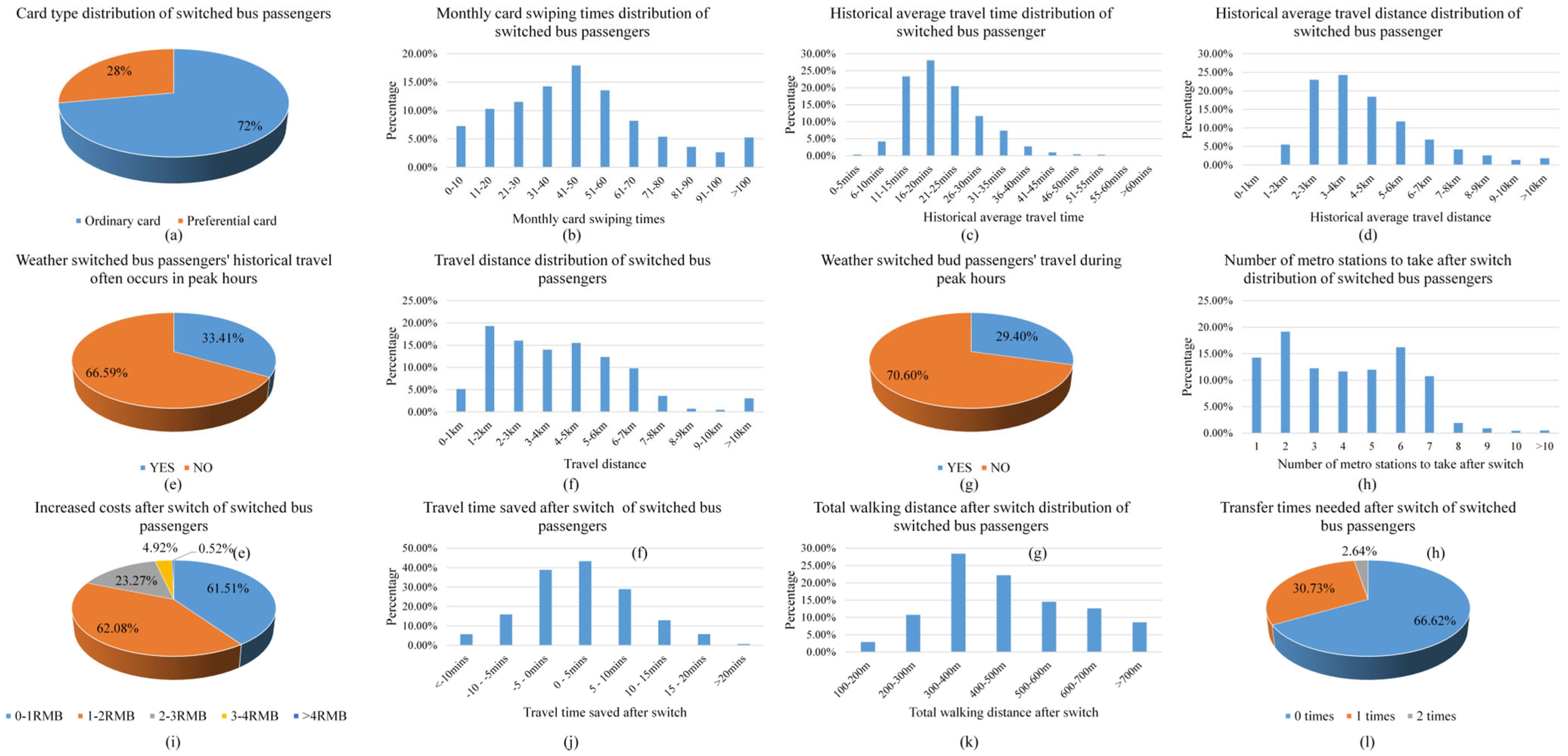
The distribution of characteristics of switched bus passengers is shown in Figure 4. The ‘card type’ of switched bus passengers is mainly ordinary cards, accounting for 72%, and most of the monthly swiping frequencies of switched bus passengers are within 10–60 times, reaching 68%. In addition, most of the switched passengers’ historical average travel times are between 10 and 25 min, and historical average travel distance is between 2 and 5 km. The switched bus passengers also do not travel frequently in peak hours. The travel distance of the switched bus passengers is mostly between 1 and 7 km, accounting for 87%. In addition, most of the passengers’ switching occurs in off-peak hours, accounting for 70.6%, and most of the switched bus passengers take metro stations less than seven times. As can be seen from Figure 4i, the increased costs after switching for the bus passengers are mostly less than RMB 2, accounting for 81%. Contrary to our intuition, we found that the travel time of some switched bus passengers did not decrease after the switch, accounting for 39.8%. As can be seen from Figure 4k, the walking distance of switched bus passengers after the switch is mostly 300–500 m. As for transfer times after the switch, most switched bus passengers do not need to transfer after switching, accounting for 66.62%, 30.73% of the switched passengers need to transfer once, and only 2.64% of the switched passengers need to transfer twice.

4.2.3. Bus Passengers’ Switch Behavior Model Based on CART Decision Tree

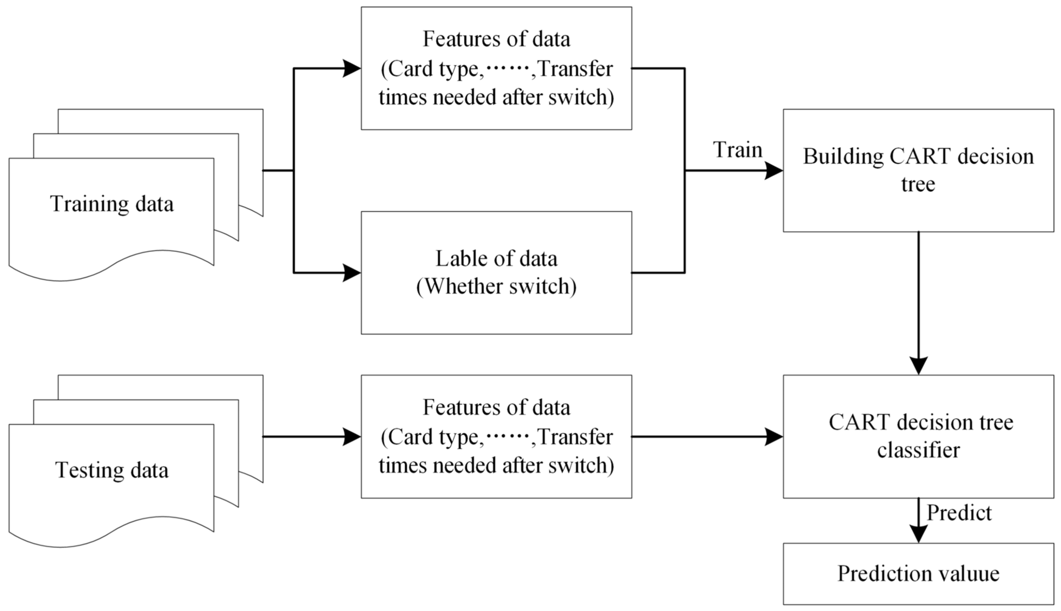
The decision tree is a basic method for classification and regression. The main advantage of decision tree model is its readability and fast classification speed. The CART decision tree was proposed by Reiman et al. [48] in 1984 and is widely used in the field of statistics. It uses bisection recursive segmentation technology to build a decision tree with a binary tree structure. Bisection recursive segmentation technology means that at the nodes where samples need to be divided, the current samples are divided into two sub samples, so that the non-leaf nodes of the decision tree have two branches. Therefore, it solves the value bias defect in the ID3 algorithm when selecting attributes with information gain. Because CART is a binary tree, it has a faster operation speed than ID3 and C4.5. At present, the CART decision tree has been widely used in many fields [54]. The bus passenger switch prediction problem requires not only good prediction accuracy, but also good interpretability to study people’s switch behavior. Hence, the CART decision tree is well suited to this field. This paper uses the 12 influencing factors extracted in the previous chapter as the input features of the model, and builds a bus passengers’ switch behavior model based on the CART decision tree, as shown in Figure 5.
In the CART algorithm, the Gini index is used as the basis of attribute selection. The Gini index is a measure of sample purity. The smaller the value, the purer it is. For a given sample set D , its Gini index is expressed as follows:
G i n i D = 1 k = 1 p k 2
Among them, p k is defined as the proportion of data points belonging to class k in the current node. The Gini index can effectively measure the effectiveness of each attribute for classification. When the Gini index is large, it means that the sample is nonuniform, otherwise, it means that the sample is relatively uniform. Therefore, the CART model will choose an attribute whose Gini index is relatively small after dividing the sample set. If the sample set D is divided into two subsets according to the value a of a certain attribute A , and the two subsets are represented by D 1 , D 2 , respectively; then, under the condition of attribute A, the Gini index of set D is:
G i n i D , A = a = D 1 D G i n i D 1 + D 2 D G i n i D 2
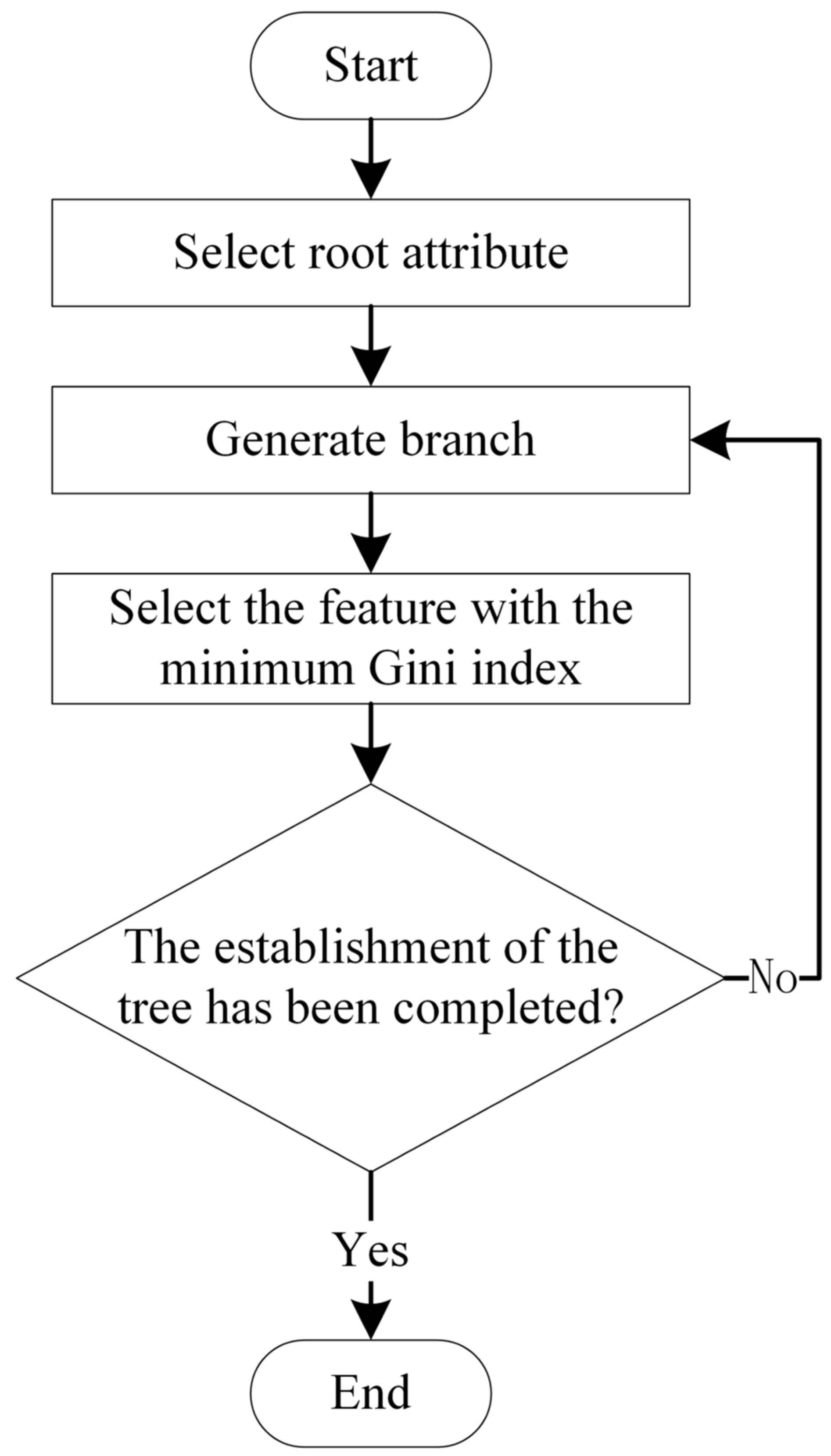
In the process of creating the CART classification decision tree, the dataset will be divided according to the different value a i of a certain feature A , and G i n i D , A = a i will be calculated according to the different divisions; then, the smallest Gini index will be found, and the value a i will be taken as the optimal cutting point of this feature. For features with continuous values, first rank the feature values in ascending order, then take the average value of adjacent feature values as possible split points, calculate the Gini index of each split point, and select the minimum value as the Gini index of the current feature. The establishment process of the CART decision tree is shown in Figure 6.

5. Experiment

5.1. Study Area and Dataset

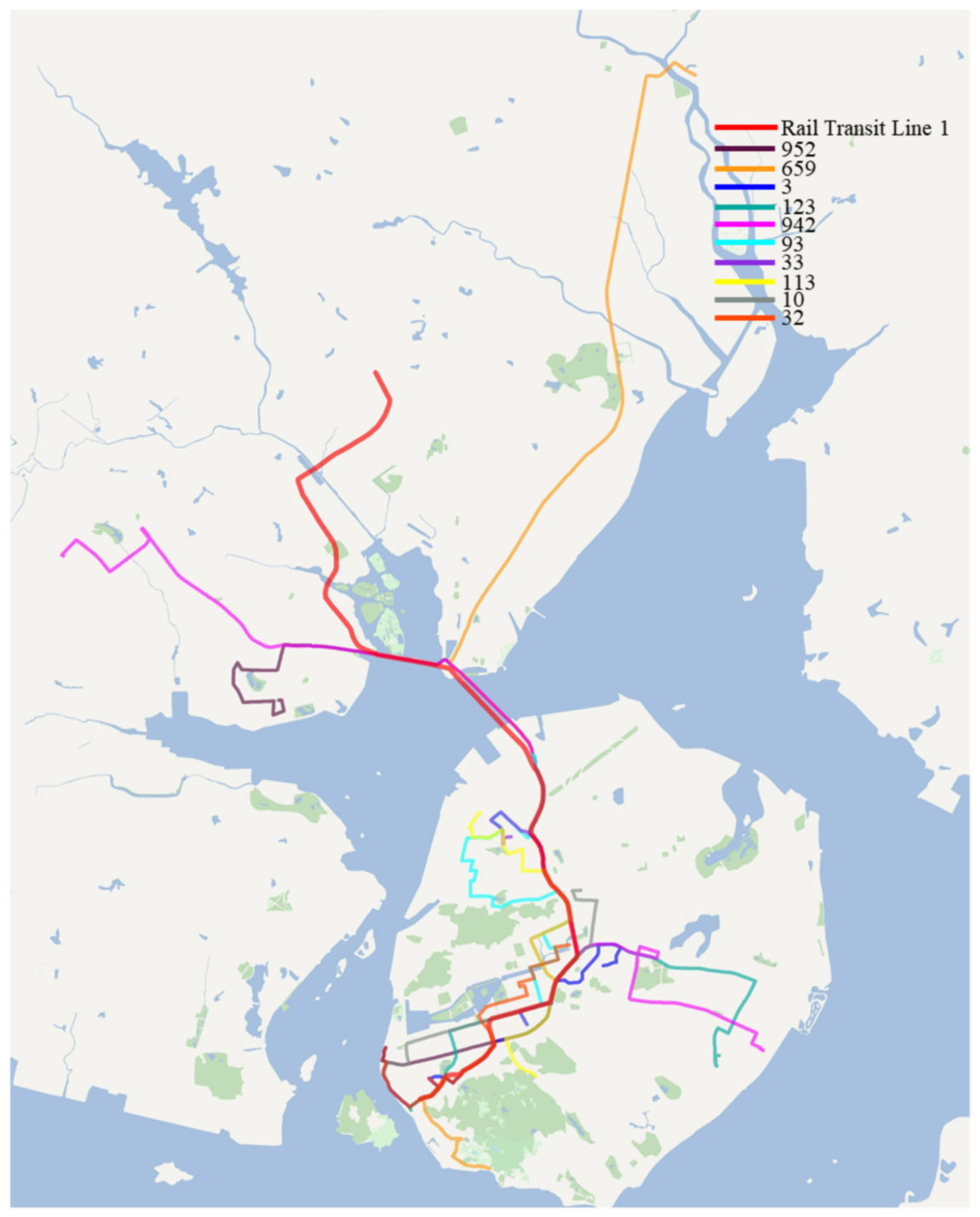
According to the switch-influencing factors dataset constructed in Chapter 4, this paper selects the switch data of 10 bus lines (‘10’, ‘113’, ‘33’, ‘93’, ‘942’, ‘123’, ‘3’, ‘32’, ‘659’, ‘952’) along the Xiamen Rail Transit Line 1 as the experimental object. The spatial relationship is illustrated in Figure 7. The total dataset consists of 5817 data points, which were divided into 4653 samples for training and 1164 for testing.

5.2. Evaluation Methods and Indicators

The primary outcome of this study is the prediction accuracy of passenger switch behavior. Secondary outcomes include (1) feature importance rankings to identify key factors influencing switch decisions, and (2) interpretable decision rules extracted from the CART model to understand passenger decision-making mechanisms.
The confusion matrix is a frequently utilized evaluation instrument in the domain of machine learning and classification problems. It is employed to illustrate the efficacy of a classification model and to present in tabular format the discrepancy between the model’s predicted labels and the actual labels on the test dataset. The confusion matrix is a two-dimensional matrix (as in Table 4) that describes the classification results of the model on the test dataset. It compares the actual labels with the predicted labels and categorizes them into four distinct categories. True Positives (TP): The number of samples in which the model predicts positive values among all samples with positive true values. False Positives (FP): The number of samples in which the model predicts a positive value among all samples with negative true values. True Negatives (TN): The number of samples in which the model predicts negative values among all samples with negative true values. False Negatives (FN): The number of samples in which the model predicts negative values among all samples with positive true values. The above definition posits that the greater the number of samples of TP and TN in the confusion matrix, the more effective the classification of the model.
The confusion matrix permits the calculation of a number of evaluation indicators, including accuracy (Acc), precision (P), recall rate (recall, R) and F1 score (F1). The larger the value of each evaluation indicators, the better the prediction result. The formulas are as follows:
A c c u r a c y = T P + T N T P + T N + F P + F N
P = T P T P + F P
R = T P T P + F N
F 1 = 2 P × R P + R
Receiver operating characteristic (ROC) analysis is commonly used to study binary classification problems. Traditionally, the area under the curve (AUC) is utilized to assess the classification performance, with the value of AUC ranging from 0 to 1. A value of AUC closer to 1 indicates a more effective classification outcome.

5.3. Experimental Setup and Statistical Validation

This section details the configuration of the comparative models and the statistical procedures employed to ensure the validity and robustness of the experimental results.

5.3.1. Parameter Configuration

Based on the data of Xiamen dataset, five models are contained in the experiment, namely logit, Naïve Bayesian (NB), Support Vector Machine (SVM), Artificial Neural Network (ANN) and CART. In this section, the hyperparameters of each model are first optimized using the GridSearchCV module from the scikit-learn library. This paper uses 5-fold cross validation method. The optimized parameters of each model are as follows:
(1) Logit: C = 1, Penalty = ‘l2’, max_iter = 1000.
(2) NB: Type= ‘Gaussian’, var_smoothing = 1 × 10⁻⁹.
(3) SVM: C = 1.0, kernel = ‘rbf’, gamma = ‘scale’.
(4) ANN: Hidden_layer_sizes = (100,100), learning_rate_init = 0.008, alpha = 0.0001.
(5) CART: Max_depth = 9, Max_leaf_nodes = 48, min_samples_split = 10, class_weight = ‘balanced’.
All other parameters were set to their default values in scikit-learn version 1.2.2.

5.3.2. Model Diagnostics and Statistical Validation

Prior to model evaluation, we conducted comprehensive diagnostic tests to validate key statistical assumptions. For all regression-based models, we calculated Variance Inflation Factors (VIF) to assess multicollinearity, with all features yielding VIF values below 5, indicating acceptable levels. For the logistic regression model specifically, we performed the Hosmer–Lemeshow goodness-of-fit test (χ2 = 8.32, p = 0.403), confirming adequate model calibration. The CART model’s assumption of independence between observations was satisfied by the data collection design, and we implemented pre-pruning to prevent overfitting.
To ensure the statistical rigor of our findings, we implemented the following measures: 95% confidence intervals for all performance metrics (Table 5) were calculated via bootstrapping with 1000 iterations; effect sizes (Cohen’s d) were computed for feature importance comparisons; and Bonferroni correction was applied to account for multiple comparisons in our significance testing (Table 6).

5.4. Experimental Results

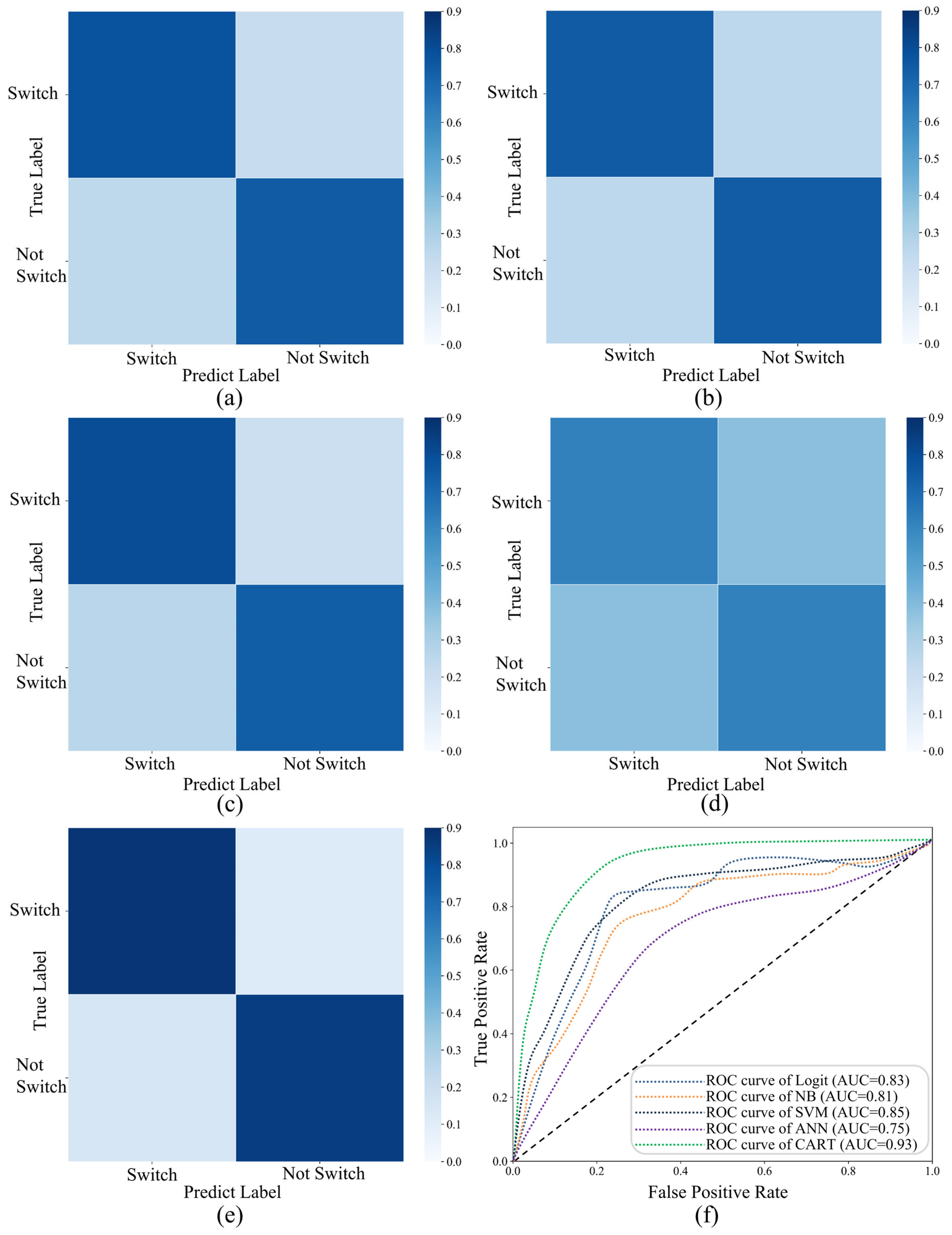
The prediction results of each model on the testing set are shown in Table 5 and Figure 8.
Referring to Table 5, the CART model has the highest accuracy of 0.85, and the prediction accuracy of logit, NB and SVM are all close to 0.8. The prediction effect of the ANN model is the worst, only 0.7, which may be related to the complex parameters of the ANN model. In terms of the precision of the model, the CART model has achieved the best prediction results in terms of the ‘switch’ precision, the ‘not switch’ precision, and the average precision. The performance of SVM model is slightly better than the logit and NB models. In the end, the prediction precision of the ANN model is still the lowest; the average precision is 0.7, while the ‘switch’ precision is only 0.67. In terms of recall, the CART model still achieves the best effect with an average recall of 0.85. We also find an interesting phenomenon that the ‘switch’ recall of all models is higher than the ‘not switch’ recall, which indicates that the model tends to predict the sample as ‘switch’. The performance of the ANN model is the most obvious, as its ‘switch’ recall is 0.81 and ‘not switch’ recall is only 0.58. In addition, the CART model has the best prediction effect in terms of the F1 score of the model, with an average F1 score of 0.84. The F1 score of logit, NB, and SVM is close to 0.78. The performance of the ANN model is the worst, as the average F1 score is only 0.69.
Furthermore, the normalized confusion matrix of each model as shown in Figure 8, indicate that the CART model achieved the best classification performance. As illustrated in Figure 8e, the CART model exhibited the highest proportion of true positives (TP) and true negatives (TN) in its confusion matrix. The receiver operating characteristic (ROC) curve of the model is depicted in Figure 8f. The CART model exhibited the highest area under the curve (AUC) value, reaching 0.93, which was significantly higher than the other four models. To sum up, the CART model has achieved the best prediction effect in each evaluation indicator, logit, NB, and SVM have similar prediction effects as a whole, and ANN model has the worst performance.
To rigorously evaluate the superiority of the proposed CART model and address its generalization capability, we conducted comprehensive comparisons and robustness checks. The CART model achieved the highest accuracy (85%), and paired t-tests confirmed that its performance improvement over the best baseline model (SVM) was statistically significant (p < 0.01). This superiority was consistent across all performance metrics in Table 4. To further assess robustness, we performed 10-fold cross-validation, which yielded a mean accuracy of 84.2% (SD = 1.5%) for CART, again outperforming all benchmarks. Additionally, experiments with an alternative train–test split (70-30) produced highly consistent results (CART accuracy: 84.7%). The statistical significance of these differences is detailed in Table 6. In summary, the CART model has achieved the best prediction effect across all evaluation metrics, demonstrating its suitability for real-world application. The following section will leverage the interpretability of this accurate model to delve into the decision-making mechanisms of passengers and derive practical insights.

5.5. Interpretation of Switching Mechanisms and Practical Implications

Building upon the established predictive performance of the CART model, this section leverages its interpretability to uncover the underlying decision-making mechanisms of passengers and derive actionable insights for public transport management.

5.5.1. Decision Rules and Factor Importance from the CART Model

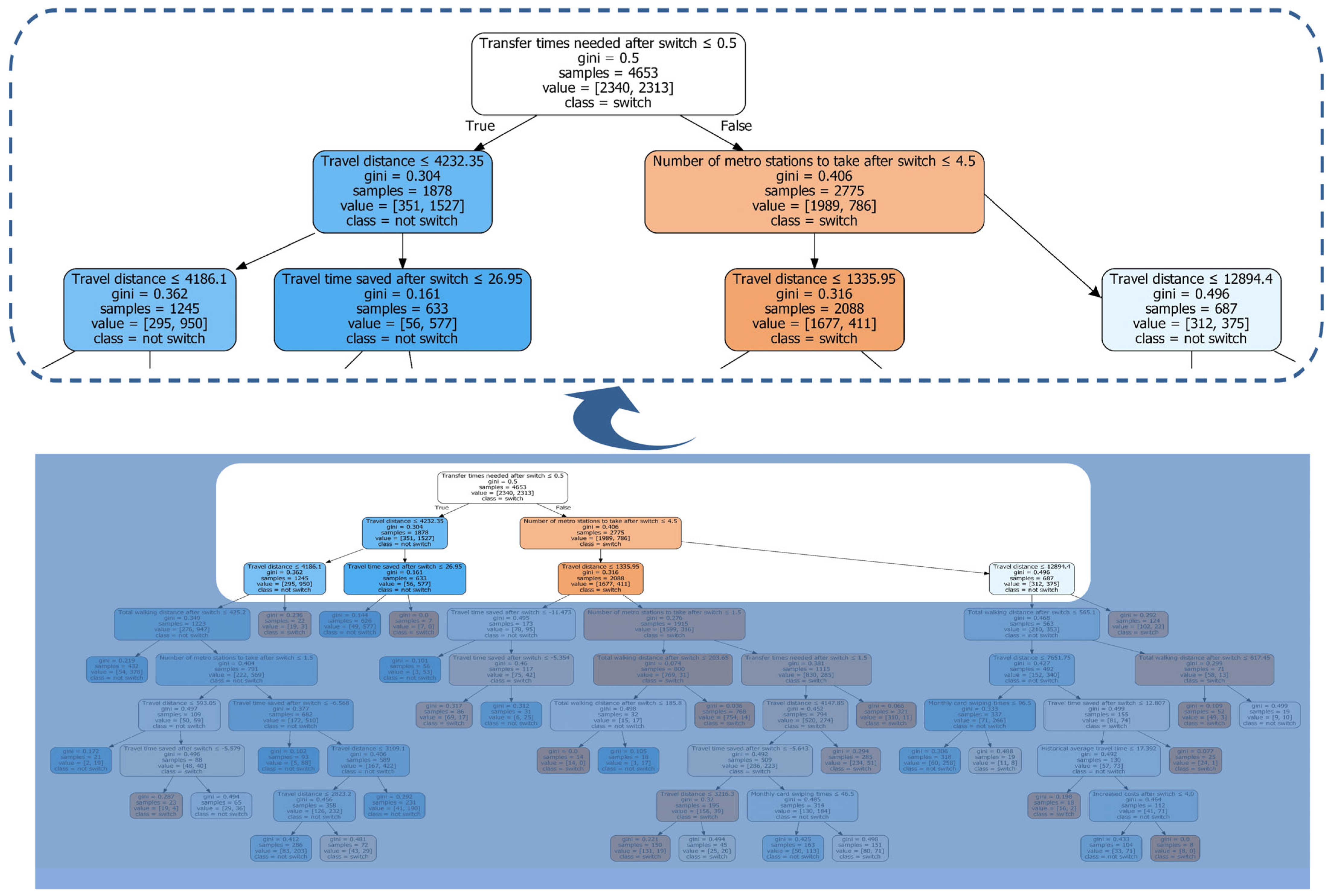
In this section, we will combine the CART model structure to analyze the people’s transfer decision-making behavior. The structure of the CART we built in the previous chapter is shown in Figure 9. In the figure, the first row of non-leaf node is the selected feature judgment standard; its left subtree (left down arrow) is the sample set whose condition is true, and its right subtree (right down arrow) is the sample set whose condition is false. The ‘Gini’ in the second row is the Gini index introduced earlier, which represents the Gini index of all samples of the current node. The ‘samples’ in the third row represent the number of samples of the current node. The ‘value’ in the fourth row indicates the number of ‘switch’ samples and the number of ‘not switch’ samples of the node. When classifying, the node category is divided into the category with more samples. The ‘class’ in the fifth row represents the category of the node as mentioned before. Because of the visual description, different output result categories are represented by different colors (orange for ‘switch’, blue for ‘not switch’). In this algorithm, nodes can be impure, and the purer the node, the darker the color.
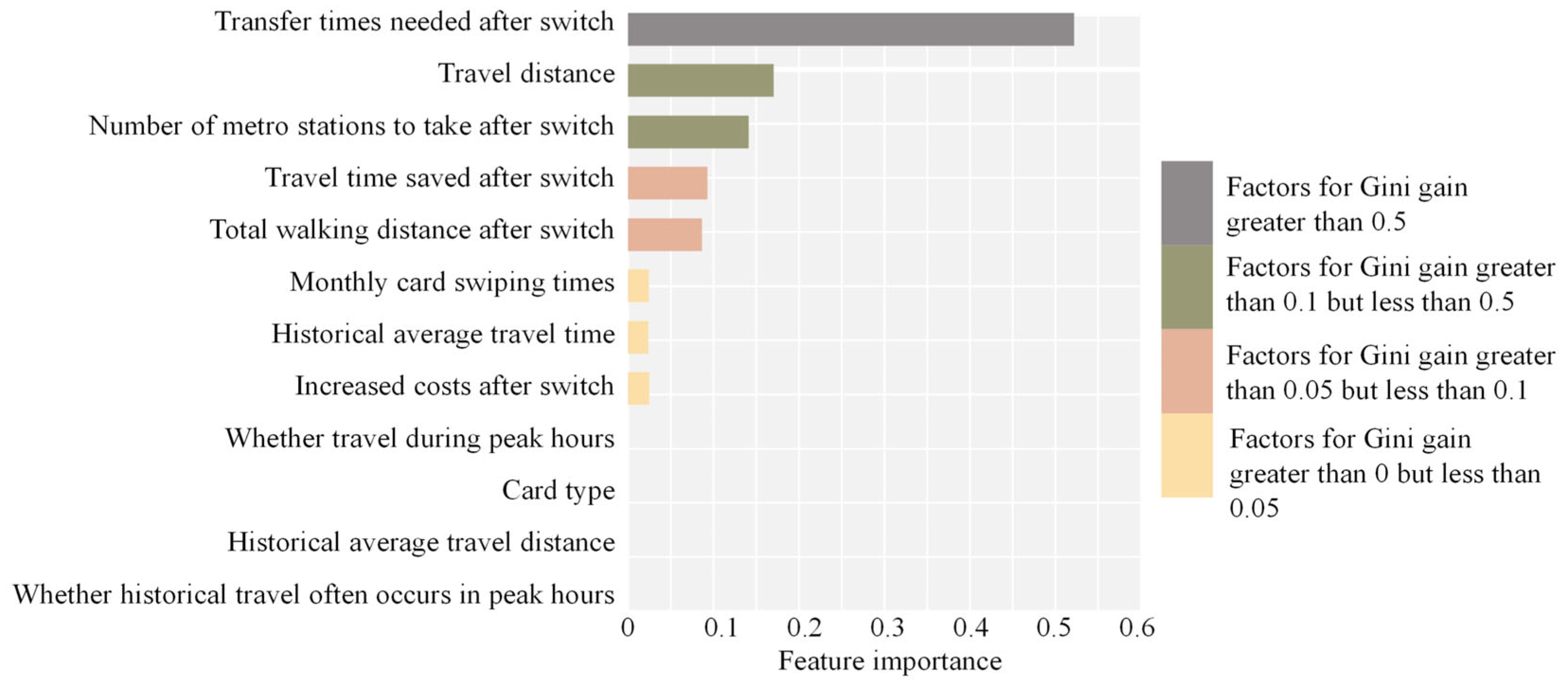
As can be seen from Figure 9, for bus passenger switch behavior, the first influencing factor is ‘Transfer times needed after switch’, which is located at the root node. The secondary influencing factors are ‘Travel distance’ and ‘Number of metro stations to take after switch’, which are located in the second layer of the tree. The third influencing factor is ‘Travel time saved after switch’, which is located in the third layer of the tree. Beyond statistical significance, we calculated effect sizes using Cohen’s d to quantify the magnitude of differences in feature importance. The top-ranked feature, ‘Transfer times needed after switch,’ demonstrated a large effect size (d = 0.82), while ‘Travel distance’ and ‘Number of metro stations’ showed medium-to-large effects (d = 0.61 and d = 0.58, respectively). This confirms that ‘Transfer times’ is not only the most statistically significant factor but also the one with the greatest practical impact on passenger switch behavior. In order to better quantify the effect of each influencing factor, this paper uses the sum of Gini gains brought by each influencing factor in the tree-creating process as the basis from which to measure the importance of features, and the order of feature importance is shown in Figure 10.
As can be seen from Figure 10, the first-ranked feature is ‘Transfer times needed after switch’, and its feature importance reaches 0.52, which is much higher than the second. This shows that the transfer times play a very important role in the switch of bus passengers. The second-ranked feature is ‘Travel distance’, with a feature importance of 0.16. The third-ranked feature is ‘Number of metro stations to take after switch’, with a feature importance of 0.14. It can be seen here that the quantitative ranking of feature importance is also consistent with our previous description of the order of influence factors. The fourth-ranked feature, ‘Travel time saved after switch’, and the fifth-ranked feature, ‘Total walking distance after switch’, have similar feature importance, 0.09 and 0.07, respectively. The features of ‘Monthly card swiping times’, ‘Historical average travel time’, and ‘Increased costs after switch’ have the same importance, which is only 0.01, indicating that these three features have a certain degree of impact on the transfer of bus passengers, but they have little effect. The remaining four features, ‘Whether travel during peak hours’, ‘Card type’, ‘Historical average travel distance’, and ‘Whether historical travel often occurs in peak hours’ are not used in the creation, so the feature importance is 0.
The dominance of these specific features provides profound behavioral insights into passenger decision-making. The paramount importance of ‘Transfer times needed after switch’ aligns with principles from behavioral economics, such as prospect theory, where the disutility of losses (e.g., the inconvenience and uncertainty of a transfer) often outweighs the utility of equivalent gains [55,56]. Each transfer introduces not only additional walking and waiting time but also psychological costs, including the cognitive load of navigation and the perceived risk of missing a connection. Consequently, passengers exhibit a strong preference for seamless, simple journeys, valuing convenience and reliability over marginal savings in travel time or cost, especially when the absolute savings in our study context were modest for many trips.
The secondary importance of ‘Travel distance’ and ‘Number of metro stations’ reveals a nuanced trade-off. For shorter trips, the door-to-door convenience of a direct bus service often outweighs the perceived speed advantage of rail. As travel distance increases, the higher in-vehicle speed and reliability of rail transit become more attractive, justifying the initial and final walking segments. The ‘Number of metro stations’ acts as a proxy for the in-vehicle rail travel time, solidifying the choice for longer-distance travelers. This interplay indicates that passengers perform a holistic evaluation of the entire journey’s complexity, comfort, and perceived efficiency, rather than simply minimizing a single factor like time or cost.
Above, we conducted an importance analysis of the features that affect the switch of bus passengers and determined that the three most important factors that affect passenger switch are ‘Transfer times needed after switch’, ‘Travel distance’, and ‘Number of metro stations to take after switch’. In addition, according to the decision tree model, this paper further analyzes the decision rules of bus passengers’ switch decision-making behavior. According to the decision tree model in Figure 9, we can see that the decision tree model generates a total of 32 leaf nodes; that is, 32 corresponding decision rules. The rules with an accuracy greater than 0.95 are shown in Table 7.

5.5.2. Practical Implications for Public Transport Planning

The behavioral insights gleaned from the CART model, particularly the passenger aversion to transfer complexity and the sensitivity to travel distance, provide a robust foundation for data-driven public transport planning and policy. The extreme importance of transfer times unequivocally indicates that the passenger’s primary sensitivity is to service integration complexity. This suggests that infrastructure and operational investments should prioritize creating seamless transfers—through measures such as co-locating bus stops and rail stations, implementing integrated ticketing systems, and optimizing schedule synchronization—as these are likely to yield higher returns in promoting mode shift than marginal reductions in fare or in-vehicle time.
Furthermore, the specific decision rules offer actionable guidance for bus network restructuring following the opening of a new rail line. According to the generated decision rules in the form of ‘If then’, it can help us more intuitively understand the switch behavior of bus passengers. The accuracy of each rule reflects the reliability of the rule. For instance, Rule 1 and Rule 10 provide clear thresholds for strategic decisions: for travel distances longer than approximately 4.2 km where significant time savings (>27 min) are possible, bus services could be strategically reduced or rerouted, as passengers are highly likely to switch. Conversely, for shorter trips where switching leads to time loss or requires multiple transfers (e.g., Rule 4, Rule 5), maintaining a robust and direct bus service is essential to retain riders.
In conclusion, the interpretability of the CART model translates predictive analytics into strategic intelligence. It enables transit authorities to identify the most impactful leverage points and design targeted, efficient, and passenger-centric policies for multimodal transport systems.

6. Conclusions and Future Work

6.1. Conclusions

We analyze passengers’ smart card data from periods before and after the rail transit line opening to construct a dataset of passenger switches. Using the switch dataset, this study extracts 12 potential influencing factors for bus passenger switches while also analyzing the characteristics of those who switched.
This paper adopts the extracted influencing factors as model input features to build a bus passenger switch behavior model using the CART decision tree algorithm. The experimental results are then evaluated using four metrics: accuracy (ACC), precision (P), recall (R), and F1 score (F1).
The results demonstrate that the CART model achieves superior predictive performance across all evaluation metrics compared to the baseline models. Finally, according to the generated tree model, this paper analyzes the sensitivity of the factors that affect the passenger switch. Our analysis identified that ‘Transfer times needed after switch’ is indeed a major factor affecting passengers’ switch, and it emerged as the primary factor in the context of Xiamen.
It is important to distinguish between our confirmatory and exploratory findings. While we hypothesized and confirmed that the CART model would provide interpretable decision rules (H2), the specific dominance of ‘Transfer times’ over traditional economic factors was an exploratory insight. In contrast to some existing studies based on survey data, our findings in Xiamen reveal that travel time and cost are not the primary factors influencing passenger transfers in this specific context. Instead, ‘Travel distance’ and ‘The number of metro stations to take after switch’ also emerge as significant determinants.
In addition, the generated tree model was used to extract ‘IF-THEN’ decision rules characterizing passenger switch behavior. These rules provide an intuitive understanding of the behavioral mechanisms. For urban transportation planners, these findings translate into several actionable strategies. The paramount importance of transfer aversion underscores the need to prioritize investments in seamless transfers through co-located stops, schedule synchronization, and integrated ticketing. Furthermore, the specific thresholds from our decision rules (e.g., the 4.2 km travel distance in Rule 1 and Rule 10) provide a data-driven foundation for bus network restructuring, enabling targeted service adjustments—such as rerouting long-distance, time-saving corridors while preserving direct bus services for shorter, transfer-intensive trips. Finally, integrating micromobility options can address last-mile connectivity challenges inherent in the modal switch. These recommendations, derived directly from passenger behavior patterns, offer a concrete framework for optimizing bus–rail integration and could assist relevant authorities in formulating more scientifically sound public transport policies. These findings offer potential insights for the adjustment of bus lines and the planning of new rail transit lines. However, the general applicability of these specific rules should be considered in light of the limitations discussed in Section 6.2.

6.2. Limitations and Future Research

While this study provides valuable insights into passenger switch behavior, several limitations pertaining to the generalizability of the findings should be acknowledged. First, the analysis is exclusively based on data from Xiamen, a medium-sized, coastal city in China with specific characteristics—such as its linear spatial layout along the coast, a significant tourism population, and a mild climate that favors year-round walking and cycling for last-mile connectivity. The city’s bus and rail transit systems, fare structure, and the specific travel habits of its residents are shaped by these unique contextual factors. Consequently, the direct applicability of our model and the identified decision rules to cities with fundamentally different urban forms (e.g., inland radial or grid-based metropolises), economic structures, or dominant travel cultures may be limited. Second, the model was trained and tested on data from ten bus lines overlapping with one primary rail corridor; its performance in complex, multi-line rail networks or in regions with different levels of transit-oriented development requires further investigation. Finally, our study, like any data-driven approach, may be subject to unobserved variable bias. Factors not captured in our dataset, such as perceptions of safety and comfort or real-time service information, could also influence switching behavior.
Future research should therefore aim to test and calibrate this approach in diverse urban contexts. A particularly promising direction is to adopt a comparative framework [57,58], applying this methodology to cities with contrasting urban forms (e.g., inland radial metropolises) and cultural backgrounds. Such a comparative analysis would serve two key purposes: (1) to systematically validate the transferability of the model and its decision rules, and (2) to investigate the universality of the identified behavioral principles, such as the dominance of transfer aversion, versus those that are context-specific. Additionally, incorporating richer data sources, including individual socio-demographic attributes and real-time service data, could further enhance our understanding of the mechanisms behind passenger decision-making. Building on this study, future work should also seek to integrate emerging travel trends and broader sustainability metrics. The growing prevalence of micromobility options (e.g., e-scooters, e-bikes) is critically reshaping last-mile connectivity and final decisions on mode of transport [7]. Incorporating these modes into the switching behavior framework will be essential for understanding and modeling modern multimodal systems. Furthermore, from a policy perspective, promoting efficient public transport integration is a key strategy for sustainable urban development. Future models could be expanded to quantify the environmental co-benefits of modal shift, such as reductions in traffic-related noise and emissions, thereby directly linking passenger behavior to broader urban sustainability goals [5].

Author Contributions

Study conception and design: Z.Z. and G.R.; data collection and processing: Z.Z., W.L., T.H. and J.S.; modeling and interpretation of results: Z.Z., T.H. and Q.C.; draft manuscript preparation: Z.Z., T.H., W.L. and C.W. Authors Z.Z. and W.L. contributed equally to the work. All authors have read and agreed to the published version of the manuscript.

Funding

This research was supported by the financial support for the National Natural Research Foundation of China (Grant No. 52202399, 52372314 and 52432010), China Postdoctoral Science Foundations (Grant No. 2022M710679) and Postgraduate Research & Practice Innovation Program of Jiangsu Province (KYCX22_0286).

Data Availability Statement

The raw smart card data that support the findings of this study are property of the Xiamen Transportation Bureau and are not publicly available due to data-sharing agreements that protect passenger privacy and urban transport operation details. The processed dataset generated for model training and the analysis code (Python 3.7 scripts) are available from the author, Zhe Zhang, upon reasonable request, subject to review and a formal data sharing agreement.

Conflicts of Interest

The authors declare no conflicts of interest.

References

  1. Juan de Dios, O. Future transportation: Sustainability, complexity and individualization of choices. Commun. Transp. Res. 2021, 1, 100010. [Google Scholar] [CrossRef]
  2. Guiding Opinions of the State Council on the Priority of Urban Development of Public Transport. Available online: http://www.gov.cn/zwgk/2013-01/05/content_2304962.htm (accessed on 29 December 2012).
  3. Peled, I.; Lee, K.; Jiang, Y.; Dauwels, J.; Pereira, F.C. On the Quality Requirements of Demand Prediction for Dynamic Public Transport. Commun. Transp. Res. 2020, 1, 100008. [Google Scholar] [CrossRef]
  4. Sun, G.; Zhao, J.; Webster, C.; Lin, H. New metro system and active travel: A natural experiment. Environ. Int. 2020, 138, 105605. [Google Scholar] [CrossRef]
  5. Danilevičius, A.; Karpenko, M.; Křivánek, V. Research on the noise pollution from different vehicle categories in the urban area. Transport 2023, 38, 1–11. [Google Scholar] [CrossRef]
  6. Majumder, S.; Singh, A.; Singh, A.; Karpenko, M.; Sharma, H.K.; Mukhopadhyay, S. On the analytical study of the service quality of Indian Railways under soft-computing paradigm. Transport 2024, 39, 54–63. [Google Scholar] [CrossRef]
  7. Karpenko, M.; Prentkovskis, O.; Skačkauskas, P. Analysing the impact of electric kick-scooters on drivers: Vibration and frequency transmission during the ride on different types of urban pavements. Eksploat. Niezawodn.-Maint. Reliab. 2025, 27, 1–14. [Google Scholar] [CrossRef]
  8. Emmanouil, C.; Mohamed, A.; Constantinos, A.; Konstadinos, G. Investigating social media spatiotemporal transferability for transport. Commun. Transp. Res. 2022, 2, 100081. [Google Scholar] [CrossRef]
  9. Anwar, A.; Oakil, A.T.; Muhsen, A.; Arora, A. What Would it Take for the People of Riyadh City to Shift from Their Cars to the Proposed Metro? Soc. Sci. Res. Netw. 2023, 12, 101008. [Google Scholar] [CrossRef]
  10. Pan, L.; Waygood, E.; Patterson, Z. Public Transit Itinerary Choice Analysis Considering Various Incentives. Transp. Res. Rec. 2023, 2677, 722–733. [Google Scholar] [CrossRef]
  11. Elharoun, M.; El-Badawy, S.; Shahdah, U. Artificial Intelligence Techniques for Predicting Individuals’ Mode Choice Behavior in Mansoura City, Egypt. Transp. Res. Rec. 2023, 2677, 605–623. [Google Scholar] [CrossRef]
  12. Nuzzolo, A.; Comi, A. Advanced public transport and intelligent transport systems: New modelling challenges. Transp. A Transp. Sci. 2016, 12, 674–699. [Google Scholar] [CrossRef]
  13. Zhang, W.; Qi, Y.; Henrickson, K.; Tang, J.; Wang, Y. Vehicle traffic delay prediction in ferry terminal based on Bayesian multiple models combination method. Transp. A Transp. Sci. 2017, 13, 467–490. [Google Scholar] [CrossRef]
  14. Yin, H.; Wu, J.; Liu, Z.; Yang, X.; Qu, Y.; Sun, H. Optimizing the release of passenger flow guidance information in urban rail transit network via agent-based simulation. Appl. Math. Model. 2019, 72, 337–355. [Google Scholar] [CrossRef]
  15. Chen, E.; Luo, Q.; Chen, J.; He, Y. Understanding passenger travel choice behaviours under train delays in urban rail transits: A data-driven approach. Transp. B Transp. Dyn. 2023, 11, 1496–1524. [Google Scholar] [CrossRef]
  16. Hollander, Y.; Prashker, J.N. The applicability of non-cooperative game theory in transport analysis. Transportation 2006, 33, 481–496. [Google Scholar] [CrossRef]
  17. Ting, L. Study on Passenger Flow Diversion Between Regular Public Transit and Proposed Rail Transit Based on Discrete Choice Model. Ph.D. Thesis, Chang’an University, Xi’an, China, 2011. [Google Scholar]
  18. Jiabin, L. Research on the Method of Bus Transit Network Adjustment in the Initial Operation of Urban Rail Transit. Ph.D. Thesis, Southest University, Dhaka, Bangladesh, 2015. [Google Scholar]
  19. Liang, L.; Wu, J.; Wang, H. Competition Model between Urban Rail and Bus Transit. Urban Mass. Transit. 2009, 7, 30–34. [Google Scholar]
  20. Wang, K.; Bhat, C.; Ye, X. A multinomial probit analysis of shanghai commute mode choice. Transportation 2022, 50, 1471–1495. [Google Scholar] [CrossRef]
  21. Harrington, A.; Parolin, B. Factors affecting the use of bus and rail services in a deregulated environment. Transportation 1991, 18, 175–193. [Google Scholar] [CrossRef]
  22. Murat, Y.S.; Cakici, Z. Comparative Analysis of Public Transport Users’ Perception Targeting Sustainable Transportation. In Engineering Tools and Solutions for Sustainable Transportation Planning; IGI Global: Hershey, PA, USA, 2017; pp. 76–98. [Google Scholar]
  23. Wang, Y.; Li, L.; Wang, Z.; Lv, T.; Wang, L. Mode Shift Behavior Impacts from the Introduction of Metro Service: Case Study of Xi’an, China. J. Urban Plan. Dev. 2013, 139, 216–225. [Google Scholar] [CrossRef]
  24. Cats, O. Identifying human mobility patterns using smart card data. Transp. Rev. 2024, 44, 213–243. [Google Scholar] [CrossRef]
  25. Oliveira, L.K.d.; Isler, C.A.; Balieiro, G.; Carvalho, T.L.L.; Littig, M.A. Bus Line Shift Behaviour: Evidence of Influential Factors based on Smart Card Data. Res. Transp. Bus. Manag. 2024, 52, 101073. [Google Scholar] [CrossRef]
  26. Ozer, F.C.; Tuydes-Yaman, H.; Dalkic-Melek, G. Increasing the precision of public transit user activity location detection from smart card data analysis via spatial–temporal DBSCAN. Data Knowl. Eng. 2024, 153, 102343. [Google Scholar] [CrossRef]
  27. Klar, R.; Rubensson, I. Spatio-Temporal Investigation of Public Transport Demand Using Smart Card Data. Appl. Spat. Anal. Policy 2024, 17, 241–268. [Google Scholar] [CrossRef]
  28. Ruiz, E.; Yushimito, W.F.; Aburto, L.; de la Cruz, R. Predicting passenger satisfaction in public transportation using machine learning models. Transp. Res. Part A Policy Pract. 2024, 181, 103995. [Google Scholar] [CrossRef]
  29. Nguyen, S.-T.; Moeinaddini, M.; Saadi, I.; Cools, M. Unveiling the drivers of modal switch from motorcycles to public transport in Southeast Asia. Transp. Res. Part F Traffic Psychol. Behav. 2024, 102, 373–391. [Google Scholar] [CrossRef]
  30. Nguyen-Phuoc, D.Q.; Currie, G.; De Gruyter, C.; Young, W. How do public transport users adjust their travel behaviour if public transport ceases? A qualitative study. Transp. Res. Part F Traffic Psychol. Behav. 2018, 54, 1–14. [Google Scholar] [CrossRef]
  31. Jian, W.; Liu, X.; Liu, H.; Hu, Y.; Gao, L. The Impacts of the Multiscale Built Environment on Commuting Mode Choice: Spatial Heterogeneity, Moderating Effects, and Implications for Demand Estimation. J. Adv. Transp. 2023, 2023, 9346631. [Google Scholar] [CrossRef]
  32. Zhou, W.; Li, X.; Shi, Z.; Yang, B.-T.; Chen, D. Impact of Carpooling under Mobile Internet on Travel Mode Choices and Urban Traffic Volume: The Case of China. Sustainability 2023, 15, 6595. [Google Scholar] [CrossRef]
  33. Deng, Y.J.; Bai, Y.; Cui, L.B.; He, R.J. Travel Mode Choice Behavior for High-Speed Railway Stations Based on Multi-Source Data. Transp. Res. Rec. 2023, 2677, 525–540. [Google Scholar] [CrossRef]
  34. Ma, S.; Yu, Z.; Liu, C. Nested Logit Joint Model of Travel Mode and Travel Time Choice for Urban Commuting Trips in Xi’an, China. J. Urban Plan. Dev. 2020, 146, 04020020. [Google Scholar] [CrossRef]
  35. Liu, L.X.; Wang, Y.J.; Hickman, R. How Rail Transit Makes a Difference in People’s Multimodal Travel Behaviours: An Analysis with the XGBoost Method. Land 2023, 12, 675. [Google Scholar] [CrossRef]
  36. Zhang, Y.; Xie, Y. Travel Mode Choice Modeling with Support Vector Machines. Transp. Res. Rec. 2008, 2076, 141–150. [Google Scholar] [CrossRef]
  37. Mane, A.S.; Sarkar, A.K.; Arkatkar, S.S.; Bhaskar, A. Effect of bus-lane usage by private vehicles on modal shift. Proc. Inst. Civ. Eng.-Transp. 2018, 171, 85–97. [Google Scholar] [CrossRef]
  38. Pineda-Jaramillo, J.; Arbeláez-Arenas, Ó. Assessing the Performance of Gradient-Boosting Models for Predicting the Travel Mode Choice Using Household Survey Data. J. Urban Plan. Dev. 2022, 148, 04022007. [Google Scholar] [CrossRef]
  39. Özuysal, M.; Tayfur, G.; Tanyel, S. Passenger flows estimation of light rail transit (LRT) system in Izmir, Turkey using multiple regression and ANN methods. Promet-Traffic Transp. 2012, 24, 1–14. [Google Scholar] [CrossRef]
  40. Ashik, F.R.; Sreezon, A.I.Z.; Rahman, M.H.; Zafri, N.M.; Labib, S.M. Built environment influences commute mode choice in a global south megacity context: Insights from explainable machine learning approach. J. Transp. Geogr. 2024, 116, 103828. [Google Scholar] [CrossRef]
  41. Jin, C.-J.; Luo, Y.; Wu, C.; Song, Y.; Li, D. Exploring the Pedestrian Route Choice Behaviors by Machine Learning Models. ISPRS Int. J. Geo-Inf. 2024, 13, 146. [Google Scholar] [CrossRef]
  42. Yin, G.; Huang, Z.; Fu, C.; Ren, S.; Bao, Y.; Ma, X. Examining active travel behavior through explainable machine learning: Insights from Beijing, China. Transp. Res. Part D Transp. Environ. 2024, 127, 104038. [Google Scholar] [CrossRef]
  43. Zhao, Y.; Stewart, K. Analyzing travel behavior differences across population groups: An explainable machine learning approach with big mobility data. J. Transp. Geogr. 2025, 128, 104368. [Google Scholar] [CrossRef]
  44. Tamim Kashifi, M.; Jamal, A.; Samim Kashefi, M.; Almoshaogeh, M.; Masiur Rahman, S. Predicting the travel mode choice with interpretable machine learning techniques: A comparative study. Travel. Behav. Soc. 2022, 29, 279–296. [Google Scholar] [CrossRef]
  45. Dwivedi, R.; Dave, D.; Naik, H.; Singhal, S.; Omer, R.; Patel, P.; Qian, B.; Wen, Z.; Shah, T.; Morgan, G.; et al. Explainable AI (XAI): Core Ideas, Techniques, and Solutions. ACM Comput. Surv. 2023, 55, 194. [Google Scholar] [CrossRef]
  46. Rudin, C. Stop explaining black box machine learning models for high stakes decisions and use interpretable models instead. Nat. Mach. Intell. 2019, 1, 206–215. [Google Scholar] [CrossRef]
  47. Islam, M.R.; Ahmed, M.U.; Barua, S.; Begum, S. A Systematic Review of Explainable Artificial Intelligence in Terms of Different Application Domains and Tasks. Appl. Sci. 2022, 12, 1353. [Google Scholar] [CrossRef]
  48. Breiman, L.; Friedman, J.; Olshen, R.A.; Stone, C.J. Classification and Regression Trees; Wadsworth International Group: Monterey, CA, USA, 1984; p. 358. [Google Scholar]
  49. Hagenauer, J.; Helbich, M. A comparative study of machine learning classifiers for modeling travel mode choice. Expert Syst. Appl. 2017, 78, 273–282. [Google Scholar] [CrossRef]
  50. Xie, C.; Lu, J.; Parkany, E. Work Travel Mode Choice Modeling with Data Mining: Decision Trees and Neural Networks. Transp. Res. Rec. 2003, 1854, 50–61. [Google Scholar] [CrossRef]
  51. Ziwei, C.; Cheng, W.; Delei, C.; Lei, L. Alighting stop determination of transit passengers based on expanded history trip records. J. Nanjing Univ. 2020, 56, 227–235. [Google Scholar] [CrossRef]
  52. Cui, J.; Gao, Y.; Cheng, J.; Shi, L. Study on the Selection Model of Staying Adjustment Bus Lines along Rail Transit. J. Adv. Transp. 2020, 2020, 6385359. [Google Scholar] [CrossRef]
  53. Board, T.R. Highway Capacity Manual; TRB: Washington, DC, USA, 2000. [Google Scholar]
  54. Wu, J.; Yang, M.; Rasouli, S.; Cheng, L. Investigating Commuting Time Patterns of Residents Living in Affordable Housing: A Case Study in Nanjing, China. Promet-Traffic Transp. 2019, 31, 423–433. [Google Scholar] [CrossRef]
  55. Kahneman, D.; Tversky, A. Prospect Theory: An Analysis of Decision Under Risk. In Handbook of the Fundamentals of Financial Decision Making; World Scientific Handbook in Financial Economics Series; World Scientific: Singapore, 2012; Volume 4, pp. 99–127. [Google Scholar]
  56. Givoni, M.; Rietveld, P. The access journey to the railway station and its role in passengers’ satisfaction with rail travel. Transp. Policy 2007, 14, 357–365. [Google Scholar] [CrossRef]
  57. Xia, C.; Zhang, A.; Yeh, A.G.O. The Varying Relationships between Multidimensional Urban Form and Urban Vitality in Chinese Megacities: Insights from a Comparative Analysis. Ann. Am. Assoc. Geogr. 2022, 112, 141–166. [Google Scholar] [CrossRef]
  58. Mutavdžija, M.; Kovačić, M.; Buntak, K. Moving towards Sustainable Mobility: A Comparative Analysis of Smart Urban Mobility in Croatian Cities. Sustainability 2024, 16, 2004. [Google Scholar] [CrossRef]
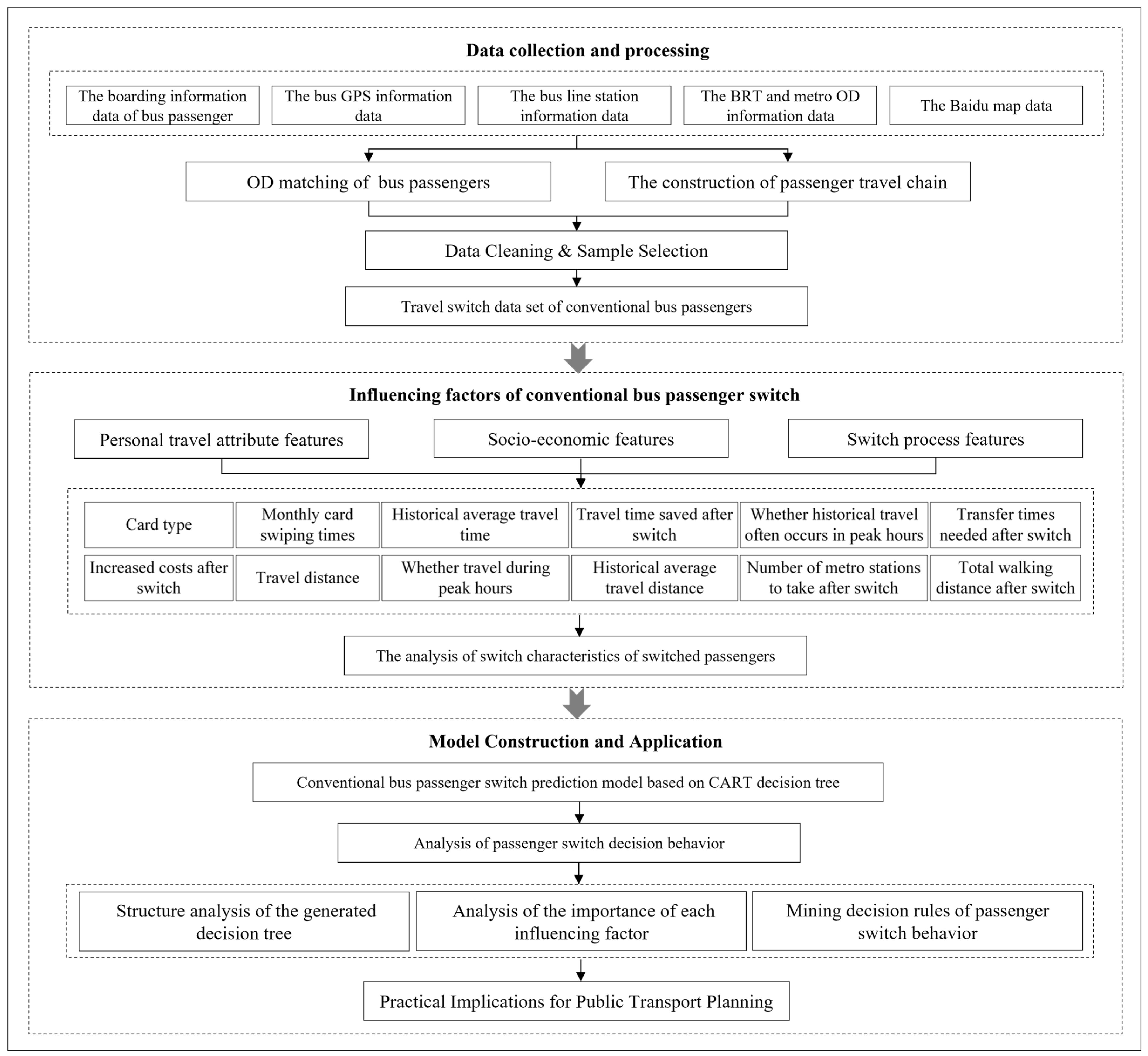
Figure 1. The technical roadmap for research.
Systems 13 00951 g001
Figure 2. A schematic of the collinear relationship between bus and the rail transit line.
Systems 13 00951 g002
Figure 3. The process of passenger switch dataset construction (with key sample sizes indicated) [51].
Systems 13 00951 g003
Figure 4. The distribution of the characteristics of switched bus passengers.
Systems 13 00951 g004
Figure 5. Bus passenger switch behavior model based on CART decision tree.
Systems 13 00951 g005
Figure 6. The establishment process of the CART decision tree.
Systems 13 00951 g006
Figure 7. The spatial location relationship between Xiamen Rail Transit Line 1 and 10 bus lines along rail transit.
Systems 13 00951 g007
Figure 8. Normalized confusion matrices and ROC curves for all models. (a) Logit; (b) NB; (c) SVM; (d) ANN; (e) CART; (f) ROC curve.
Systems 13 00951 g008
Figure 9. Visual CART decision tree of bus passengers’ switch behavior.
Systems 13 00951 g009
Figure 10. Ranking of the importance of influencing factors.
Systems 13 00951 g010
Table 1. Comparative analysis of methods for modeling passenger travel behavior.
Method CategoryExample ModelsTypical Data SourcesInterpretabilityPredictive AccuracyKey References
Traditional Discrete ChoiceLogitQuestionnaire (RP/SP)HighLow[19,34]
Classical Machine LearningSVM, ANNQuestionnaire, Smart CardLow to ModerateModerate[36,39]
Soft Computing/Advanced MLGradient Boosting, Fuzzy SystemsSmart Card, GPS, SensorsLow to Moderate (model-dependent)High[41,42]
Our Proposed MethodCART Decision TreeSmart CardHighHighThis Study
Table 2. Travel switch dataset of bus passengers in November 2017.
Card NumberDateBus Line NumberBoarding TimeBoarding StopAlighting TimeAlighting StopWhether SwitchSwitch ModeTravel Chain After Switch
(Line Number: Boarding Station, Alighting Station)
01**892017/11/1965920:32:55Lvcuobei20:48:29JiangjunciYesRail transit(rail line 1: Lvcuo, Jiangjunci)
19**652017/11/1212307:13:32Caitang school08:18:43Fuyoubai
jianyuan
NoBus + Rail transit(123: Caitang school, Zhiwuyuan)—(rail line 1: Lvcuo, Zhenhailu)
15**372017/11/3094218:41:01Lvcuobei19:18:18Xingbei
xincheng
YesRail transit + Bus(rail line 1: Lvcuo, Yuanboyuan)—(942: Yuanboyuan, Xingbeixincheng)
82**162017/11/2865908:10:15Yuekouxiaoqu09:48:03Jinbang
park
YesBus + Rail transit + Bus(659: Yuekouxiaoqu, Zhongpu)—(rail line 1: Gaoqi, Lianban)—(659: Lianbanguomao, Jingbang park)
Note: The ‘**’ represents encrypted numbers.
Table 3. Descriptions of the values of each influencing factor.
Influencing FactorDescription
Card typeOrdinary card: 0, Preferential: 1.
Monthly card swiping timesCard swiping times of the passenger in November 2017.
Historical average travel timeHistorical average travel time of the passenger in November 2017 (measured in minutes).
Historical average travel distanceHistorical average travel distance of the passenger in November 2017 (measured in meters).
Whether historical travel often occurs in peak hoursWhether more than half of the passenger’s trips occurred during peak hours. 1 represents yes, 0 represents no.
Travel distanceThe travel distance of the OD.
Whether travel during peak hours1 represents yes, 0 represents no.
Number of metro stations to take after switchThe number of metro stations the passenger will take after switching.
Increased costs after switchThe increased travel cost of the passenger after switching (measured in RMB).
Travel time saved after switchThe saved travel cost of the passenger after switching (measured in minutes).
Total walking distance after switchIt includes the walking distance of getting to the station and the walking distance needed for transfer (measured in minutes).
Transfer times needed after switchThe needed transfer times of the passenger after switching.
Whether switch1 represents yes, 0 represents no.
Table 4. Confusion matrix.
Predicted as Positive ValuePredicted as Negative Value
Positive true valueTrue Positives (TP)False Negatives (FN)
Negative true valueFalse Positives (FP)True Negatives (TN)
Table 5. Prediction results of each model (with 95% confidence intervals).
ModelsAccuracy [95% CI]TypePrecision [95% CI]Recall [95% CI]F1 Score [95% CI]
Logit0.79 [0.76–0.82]‘switch’0.78 [0.75–0.81]0.82 [0.79–0.85]0.80 [0.77–0.83]
‘not switch’0.80 [0.77–0.83]0.76 [0.73–0.79]0.78 [0.75–0.81]
average0.79 [0.76–0.82]0.79 [0.76–0.82]0.79 [0.76–0.82]
NB0.78 [0.75–0.81]‘switch’0.77 [0.74–0.80]0.81 [0.78–0.84]0.79 [0.76–0.82]
‘not switch’0.78 [0.75–0.81]0.75 [0.72–0.78]0.77 [0.74–0.80]
average0.78 [0.75–0.81]0.78 [0.75–0.81]0.78 [0.75–0.81]
SVM0.80 [0.77–0.83]‘switch’0.78 [0.75–0.81]0.84 [0.81–0.87]0.81 [0.78–0.84]
‘not switch’0.82 [0.79–0.85]0.75 [0.72–0.78]0.78 [0.75–0.81]
average0.80 [0.77–0.83]0.80 [0.77–0.83]0.79 [0.76–0.82]
ANN0.70 [0.67–0.73]‘switch’0.67 [0.64–0.70]0.81 [0.78–0.84]0.73 [0.70–0.76]
‘not switch’0.74 [0.71–0.77]0.58 [0.55–0.61]0.65 [0.62–0.68]
average0.70 [0.67–0.73]0.70 [0.67–0.73]0.69 [0.66–0.72]
CART0.85 [0.83–0.87]‘switch’0.82 [0.79–0.85]0.89 [0.87–0.91]0.86 [0.84–0.88]
‘not switch’0.87 [0.85–0.89]0.80 [0.77–0.83]0.83 [0.81–0.85]
average0.85 [0.83–0.87]0.85 [0.83–0.87]0.84 [0.82–0.86]
Note: The 95% confidence intervals (CI) were calculated using bootstrapping with 1000 iterations.
Table 6. Statistical significance testing of accuracy differences (Paired t-test with Bonferroni correction).
Comparisont-Statisticp-ValueSignificance (α = 0.01)
CART vs. Logit8.92<0.001Significant
CART vs. SVM5.41<0.001Significant
CART vs. ANN12.35<0.001Significant
CART vs. NB9.18<0.001Significant
SVM vs. Logit1.450.152Not Significant
Note: The p-values are derived from paired t-tests conducted on the accuracy results from 10-fold cross-validation. Significance was assessed at a Bonferroni-corrected α level of 0.01 to account for multiple comparisons.
Table 7. Bus passenger switch decision rules.
Sequence Number Condition ResultAccuracy
Rule 1IFTransfer times needed after switch ≤ 0.5 AND Travel distance > 4232.35 AND Travel time saved after switch > 26.95THEN‘switch’1
Rule 2IFTransfer times needed after switch > 0.5 AND Number of metro stations to take after switch ≤ 1.5 AND Travel distance > 1335.95 AND Total walking distance after switch ≤ 185.8THEN‘switch’1
Rule 3IFTransfer times needed after switch > 0.5 AND Number of metro stations to take after switch > 4.5 AND (7651.75 < Travel distance ≤ 12,894.4) AND Total walking distance after switch ≤ 565.1 AND Travel time saved after switch ≤ 12.807 AND Historical average travel time > 17.392 AND Increased costs after switch > 4.0THEN‘switch’1
Rule 4IF(0.5 < Transfer times needed after switch ≤ 1.5) AND (1.5 < Number of metro stations to take after switch ≤ 4.5) AND (1335.95 < Travel distance ≤ 3216.3) AND Travel time saved after switch ≤ −5.643 AND Historical average travel time ≤ 9.182THEN‘not switch’1
Rule 5IF(0.5 < Transfer times needed after switch ≤ 1.5) AND (1.5 < Number of metro stations to take after switch ≤ 4.5) AND (1335.95 < Travel distance ≤ 3216.3) AND Travel time saved after switch ≤ −5.643 AND Total walking distance after switch ≤ 434.4THEN‘not switch’1
Rule 6IFTransfer times needed after switch > 0.5 AND Number of metro stations to take after switch ≤ 1.5 AND Travel distance > 1335.95 AND Total walking distance after switch > 203.65THEN‘switch’0.98
Rule 7IFTransfer times needed after switch > 1.5 AND (1.5 < Number of metro stations to take after switch ≤ 4.5) AND Travel distance > 1335.95 THEN‘switch’0.97
Rule 8IFTransfer times needed after switch > 0.5 AND Number of metro stations to take after switch > 4.5 AND (7651.75 < Travel distance ≤ 12,894.4) AND Total walking distance after switch ≤ 565.1 AND Travel time saved after switch > 12.807THEN‘switch’0.96
Rule 9IFTransfer times needed after switch ≤ 0.5 AND Travel distance ≤ 4186.1 AND Total walking distance after switch > 425.2 AND Number of metro stations to take after switch > 1.5 AND Travel time saved after switch ≤ −6.568THEN‘not switch’0.95
Rule 10IFTransfer times needed after switch ≤ 0.5 AND Travel distance > 4232.35 AND Travel time saved after switch ≤ 26.95 THEN‘not switch’0.92
Rule 11IFTransfer times needed after switch > 0.5 AND Number of metro stations to take after switch ≤ 4.5 AND Travel distance ≤ 1335.95 AND Travel time saved after switch ≤ −11.473THEN‘not switch’0.95
Disclaimer/Publisher’s Note: The statements, opinions and data contained in all publications are solely those of the individual author(s) and contributor(s) and not of MDPI and/or the editor(s). MDPI and/or the editor(s) disclaim responsibility for any injury to people or property resulting from any ideas, methods, instructions or products referred to in the content.