Article

Considering Consumer Quality Preferences, Who Should Offer Trade-in Between Manufacturer and Retail Platform?

School of Business, Qingdao University, Qingdao 266071, China
*
Author to whom correspondence should be addressed.
Systems 2025, 13(11), 1043; https://doi.org/10.3390/systems13111043
Submission received: 22 October 2025 / Revised: 16 November 2025 / Accepted: 18 November 2025 / Published: 20 November 2025
(This article belongs to the Section Supply Chain Management)

Abstract

The trade-in service can enhance product sales and increase consumer loyalty; however, heterogeneity in consumer quality preferences significantly influences the provision and implementation of trade-in activities. By constructing a dynamic dual-supply chain model, this study examines the optimal choices for trade-in providers and the impact of consumer quality preferences on mode selection. The findings indicate that the decision of who should provide the trade-in service largely depends on the product’s quality decay rate. When the quality decay rate is low, collaboration between the manufacturer and the retail platform favors manufacturer-led trade-in service. Conversely, when the quality decay rate is high, both parties tend to fall into a prisoner’s dilemma, each preferring to dominate the trade-in process independently. Notably, as the share of pragmatic consumers increases, both sides of the supply chain are more inclined to prefer the manufacturer offering trade-in service. In our extended research, we found that the influence of government subsidies on mode selection primarily depends on the price discounts provided by the dominant party in trade-in arrangements within each mode. We also considered scenarios with asymmetric net residual values of recovered products, and the results robustly validate the stability of our core findings.

1. Introduction

1.1. Background and Motivation

Trade-in has long been regarded as an effective strategy to boost sales and enhance consumer loyalty. The so-called trade-in program refers to a transaction method offered by manufacturers or retail platforms that allows consumers to exchange or offset the value of their existing products when purchasing new items. From the consumer perspective, trade-in service can incentivize the purchase of new products to some extent [1,2]. From the business standpoint, the trade-in sales model can accommodate higher manufacturing costs. This model is applicable whether the service is provided by manufacturers or by retailers. Moreover, the residual value of recovered products can generate additional revenue for the company [3,4,5]. According to the latest data, over 80% of consumers prefer to use trade-in programs when purchasing the iPhone 16.1 In 2023, Haier Smart Home generated 54.8 billion yuan in sales through trade-in initiatives, accounting for 30% of its total sales.2 These figures clearly demonstrate the substantial potential of trade-in programs in driving sales growth. Furthermore, to promote the implementation of trade-in programs, governments worldwide have introduced numerous relevant policies. France has allocated over 1.3 billion euros to incentivize trade-in initiatives, while Spain announced a €3.75 billion economic stimulus plan for trade-in activities, with the first phase disbursing €1.535 billion in 2020.3
When implementing trade-in services, there are typically two primary approaches: one is the direct trade-in service provided by manufacturers (Model M), and the other is the trade-in service offered by retail platforms (Model I). Manufacturer-led trade-in programs offer the key advantage of complete control over product pricing, as the manufacturer retains full authority over market prices. All products recovered through the trade-in scheme are owned entirely by the manufacturer. In the automotive industry, approximately 40% to 57% of new vehicle sales involve trade-in programs [6,7]. Lexus launched a series of trade-in support policies targeted at Toyota owners. Benefiting from these policies, the brand achieved a cumulative sales volume of 158,000 units in the Chinese market from January to September 2020. This sales figure represents a 9.6% year-on-year increase, and it remained unaffected even amid the overall market downturn.4 Recently, Mercedes-Benz announced that starting 27 April 2024, customers participating in trade-in programs will not only receive the national one-time fixed subsidy but also be eligible for an additional subsidy of up to 15,000 yuan.5 In the trade-in services offered by retail platforms, the market price of products is set independently by the platform. For recycled items, the platform shares ownership with manufacturers based on a pre-agreed proportion. For example, Amazon’s recent trade-in program includes devices such as Kindle eReaders, headphones, and gaming consoles. The platform refurbishes or recycles old equipment, and consumers typically receive digital gift cards. If eligible, they may also benefit from additional promotional discounts.6 Since 2009, Best Buy has collected and recycled 2.7 billion pounds of electronic products and appliances, establishing itself as the largest electronic waste retail recycling platform in the United States.7 In addition to the companies mentioned above that offer trade-in services, Table 1 also provides examples of other enterprises in the industry that provide similar trade-in programs.
Based on the observed reality, both manufacturers and retail platforms have the capacity to lead the trade-in process. Consequently, a critical question arises: who should be responsible for providing trade-in service—the manufacturer or the retail platform? Building on this, the present study aims to offer theoretical guidance for the rational selection of trade-in suppliers within a dual-channel supply chain.
When faced with various options in the market, consumers make trade-offs between price and quality, resulting in differing preferences for quality levels [8]. Trade-in services are currently provided by multiple types of entities, with manufacturers and retail platforms being the primary providers. For the successful implementation of trade-in programs, a critical prerequisite must be fulfilled. Specifically, it requires understanding the heterogeneity of consumers in terms of their quality preferences and demands, and such understanding should be derived from the consumption perspective. This is because consumers’ quality preferences considerably influence their purchasing decisions [9,10]. According to the 2023 Consumer Behavior Survey Report for Double Eleven, 21.34% of consumers indicated they would continue to upgrade certain products, while others are particularly concerned with cost-performance ratio. Additionally, 12.41% of consumers plan to further upgrade their spending by purchasing higher-quality products to enhance their quality of life. Moreover, 11.78% of consumers prefer to buy durable or higher-value retention product.8 Given the heterogeneity in consumer quality preferences, consumers can be segmented into different categories, enabling more targeted provision of products and services.
Based on the analyses of consumer purchasing behavior and the development of a multidimensional influence model encompassing economic, social, and psychological factors, as referenced by Cui et al. [11], this classification corresponds to two of the most representative consumer types, each emphasizing different quality dimensions. Pragmatic consumers tend to prioritize the practicality and functionality of products. Their purchasing decisions are primarily based on the actual performance, usability, and durability of the product or service. Conversely, innovative consumers place greater emphasis on novelty and uniqueness. They are enthusiastic about exploring new and inventive products or services, focusing more on design aesthetics, creative concepts, and brand image rather than functional attributes. The most notable difference between these two groups lies in their sensitivity to product quality and their market share, which significantly influences manufacturers’ and retail platforms’ choices regarding trade-in and upgrade programs. If consumers in the market who prioritize product durability are more sensitive to quality and hold a larger market share, manufacturers are likely to adjust their product positioning by enhancing durability design and quality control measures to meet the needs of this segment. They may prefer to partner with retail platforms that dominate the used product exchange model, which allows for direct control over product quality and sales channels. Simultaneously, retail platforms may be more inclined to collaborate with such manufacturers to attract more pragmatic consumers. Conversely, when consumers seeking innovation are more sensitive to product quality and constitute a larger market share, manufacturers might opt to lead the used product exchange process themselves. This approach is often advantageous during new product launches, as it can offer more experiential opportunities such as trials and live demonstrations, which are particularly important for consumers who value product innovation. Furthermore, manufacturer-led trade-in programs are typically accompanied by enhanced product assurances, such as authenticity guarantees and comprehensive after-sales support. To attract consumers who prioritize product innovation, manufacturers and retail platforms often opt for manufacturer-driven trade-in schemes to build consumer trust. For example, Tesla, as a leader in the electric vehicle industry, primarily targets consumers seeking cutting-edge technology. Consequently, Tesla generally employs a manufacturer-led trade-in model when offering exchange services, directly selling products to consumers.9
Through the above discussion, we find that consumer quality preferences play a crucial role in the implementation of trade-in programs. However, upon reviewing relevant literature, we discovered that there are few studies that examine both aspects jointly. Therefore, we aim to address this gap in the field by investigating the following research questions:
(i)
What is the optimal decision-making and profitability of the manufacturer and the retail platform when they dominate trade-in, respectively?
(ii)
What are the implications of different quality sensitivities and market shares of consumers on the profitability of manufacturer and retail platform?
(iii)
What is the optimal trade-in model? What is the impact of considering consumer segmentation based on quality preferences on the choice of model?
To address the questions, we consider constructing a dynamic duopoly supply chain comprising a manufacturer (such as IBM or Hewlett-Packard) and a retail platform (such as Suning or Amazon), where the manufacturer sells a single type of product through the retail platform. The manufacturer undertakes product quality improvements, and both the manufacturer and the retail platform can offer trade-in service. Additionally, we categorize consumers into pragmatic and innovative types. Pragmatic consumers focus on the practicality and functionality of the product, emphasizing performance quality. Conversely, innovative consumers value the novelty and additional attributes of the product, such as feature quality, design, creativity, and brand image. For example, in the mobile phone market, pragmatic consumers focus on practical performance aspects such as call quality, durability, and battery life, while innovative consumers prioritize features like foldable screens, facial recognition, and camera resolution. We employ game theory to analyze two potential scenarios for trade-in programs: one where the manufacturer offers trade-in service (Model M) and another where the retail platform provides such service (Model I). We identify the optimal pricing and quality enhancement strategies for each trade-in model and compare them to assess how consumer segmentation influences the choice of trade-in approach. Our key findings are summarized as follows:
Firstly, in the retail platform-led trade-in resale model, a double markup effect exists from wholesale to retail prices, resulting in the market price of products in Model I exceeding that in Model M. The extent of quality improvement investment in both models depends on the net residual value of the recovered products. Secondly, we find that the larger the market share of pragmatic consumers and the more sensitive they are to quality, the lower the profits the manufacturer and the retail platform can achieve through trade-in programs. Conversely, the behavior of innovative consumers exhibits the opposite trend. Furthermore, the optimal choice of the trade-in model primarily depends on the product’s rate of quality depreciation. The retail platform tends to delegate the dominant role in trade-in to the manufacturer when the product’s quality decay rate is low, whereas they prefer to take the lead themselves when the decay rate is high. The manufacturer invariably chooses to control the trade-in process. The equilibrium where both parties are satisfied occurs when the manufacturer-led trade-in model is adopted under conditions of low product quality decay. Ultimately, the market share of different consumer segments influences the choice of the trade-in model. As the proportion of pragmatic consumers increases, the manufacturer and the retail platform tend to favor a manufacturer-led trade-in approach.

1.2. Contribution Statement and Article Structure

To our knowledge, we are the first to conduct a dynamic study that integrates consumer quality preferences with the trade-in model. Firstly, considering that consumers are highly concerned about product quality in trade-in activities, we categorize consumers into two types based on their quality preferences: the pragmatic type, who values product durability, and the innovative type, who prioritizes product novelty. We reveal how their differing levels of quality sensitivity and market share impact the profitability of manufacturers and retail platforms within the trade-in supply chain. Secondly, unlike previous studies on trade-in programs that focus on static product quality [12,13,14,15], we conceptualize the perceived quality evolution as a dynamic process. We provide a more detailed description of how long-term quality improvements influence perceived product quality. This description enables a more comprehensive characterization of two key aspects: consumer segments with different quality preferences, and the impact of these segments on market demand for trade-in products. Finally, we build on the concepts of dynamic perceived quality and consumer heterogeneity. Based on these concepts, we further examine how consumer segmentation—derived from quality preferences—influences the mode selection in trade-in programs. Through this examination, we identify the key factors that determine the choice of trade-in model.
The remainder of the paper is organized as follows. Section 2 provides a brief review of the referenced relevant literature. Section 3 describes the model and key assumptions. Section 4 gives the optimal decision as well as the optimal profit level. Section 5 describes the comparison between different strategies and performs a sensitivity analysis. Section 6 further examines the effects of model parameters on decision variables and the choice of trade-in model in the form of numerical examples. Section 7 extends the article by considering government subsidies and asymmetric net salvage value of recycled products. Section 8 summarizes the article and gives managerial insights. All proof procedures are provided in Appendix A.

2. Literature Review

This paper draws on and contributes to the literature in three areas: trade-in pricing decisions, trade-in model selection, and trade-in consumer segmentation.

2.1. Trade-in Pricing Decisions

Firstly, our article is closely related to the literature on pricing strategies involving trade-in programs. These studies typically focus on multi-period dynamic pricing, competitive strategies among firms, product remanufacturing, differential pricing, and government subsidies. Regarding optimal pricing and trade-in strategies under limited trade-in periods, Hu et al. [13] found that a firm’s optimal price generally increases with the incremental value of the product, while trade-in discounts tend to decrease as the trade-in period is extended. Yin et al. [16] developed a two-period dynamic game model that examines how manufacturers can optimize pricing strategies across two consecutive product generations through trade-in programs. This analysis considers market heterogeneity, product uncertainty, and consumers’ forward-looking behavior. Similarly, Xu, Wang, and Cao [17] analyzed how trade-in services influence the dynamic pricing and logistics decisions of durable goods companies across different sales stages (two periods).
Multiple retail competitions and product return rates influence pricing strategies within closed-loop supply chains. Competition among retailers may lead to reductions in retail and wholesale prices [18]. Ma et al. [19] conducted an in-depth analysis of pricing strategies in remanufactured product transactions, considering the dual reference effects of consumers—reference price effect and reference quality effect—and their impact on pricing decisions under different scenarios, such as with or without government subsidies and consumer rebates. Agrawal et al. [20] examined how original equipment manufacturers (OEMs) implement price discrimination through trade-in programs when offering remanufactured products and how they compete with third-party remanufacturers (3PR). When manufacturers face choices of retail partners and recycling platforms for trade-in collaborations, differential pricing strategies—where manufacturers set different wholesale prices based on partner characteristics and market positioning—benefit the manufacturers but may disadvantage retailers [21]. Li and Tian [22] analyzed the optimal pricing strategies for automotive retailers offering trade-in services under varying levels of consumer mileage anxiety. They found that pricing primarily depends on production costs, manufacturer recycling prices, and government subsidies. Both manufacturers and retailers should dynamically adjust their trade-in pricing strategies in response to changes in government support and consumer acceptance [23]. Wang et al. [24], from a supply chain financing perspective, regard the “upgrade subsidy intensity” as an implicit price discount. They found that a 1% increase in subsidies is associated with an average extension of 0.7 days in the supplier’s credit period, indicating that manufacturers employ rebate-driven pricing strategies to offer longer payable terms, thereby incentivizing consumer product replacements.

2.2. Trade-in Model Selection

Secondly, regarding the selection of suppliers for trade-in programs within the supply chain, there are diverse perspectives in academic discourse. Wang et al. [25] developed a multi-stage game-theoretic model to examine who should provide trade-in services in resale and consignment modes. They found that in the resale mode, both manufacturers and electronic retailers tend to prefer the other party to offer trade-in services, whereas in the consignment mode, both parties may reach an agreement on the preferred provider of the trade-in program, largely influenced by the commission rate. Similar conclusions are drawn by Xiao [26], who investigated the mode selection for initiating trade-in programs in centralized versus decentralized supply chains under exogenous pricing conditions. However, Quan et al. [16] established a two-period supply chain model for trade-in programs, revealing that, in most cases, supply chain members prefer to provide trade-in services themselves, and they also outlined the conditions under which each enterprise would choose to offer such services. Furthermore, Miao et al. [27] compared the economic benefits of three reverse logistics models—centralized recovery, manufacturer recovery, and retailer recovery—and found that, for manufacturers and retailers, centralized recovery outperforms retailer recovery, which in turn outperforms manufacturer recovery. In the remanufacturing context, when consumer acceptance of online direct sales channels exceeds a certain threshold, a dual-channel recovery model involving both manufacturers and retail platforms is more advantageous than the traditional retailer recovery model. Conversely, when consumer acceptance of online direct channels remains within a specific range, manufacturers tend to prefer the dual-channel approach [28]. Considering the costs associated with trade-in programs, higher costs incentivize more capable manufacturers to delegate trade-in services to retailers [4]. When green technologies are implemented concurrently with the launch of trade-in initiatives, Dou et al. [29] indicate that retail platforms acting as the primary agents in trade-in programs can generate higher supply chain profits and social welfare, although this may come at the expense of environmental sustainability.
When considering the participation of third-party recycling platforms, Fan, Guo, and Wang [14] examined whether manufacturers choose to delegate waste collection to third-party recyclers to enhance collection efficiency within retail and dual-channel structures. More recently, Zhao et al. [30] challenged the traditional hierarchical structure of supply chains, providing an in-depth analysis of the cooperative and competitive relationships between retailers and recyclers and how these dynamics influence supply chain operations and strategies. Their results indicate that recyclers always profit from autonomous recycling activities, while retailers’ profits may be compromised due to competition in the recycling market.

2.3. Trade-in Consumer Segmentation

The third domain relevant to our research pertains to consumer segmentation within trade-in services. Li et al. [31] demonstrated that considering product characteristics and consumer heterogeneity can enhance the prediction of the implementation of trade-in policies and product recovery processes. Typically, when launching a trade-in program, companies should adopt a strategic framework that differentiates between new customers and existing customers utilizing trade-in services [3]. Following Ray et al. [3], numerous researchers have further explored issues related to trade-in strategies. For instance, examining the resale of refurbished products alongside new items within limited sales cycles [32], analyzing how the second-hand market influences original equipment manufacturers (OEMs) in selecting optimal trade-in and remanufacturing strategies [33], and investigating the impact of consumer segmentation on firms’ decision-making and profitability in dual-channel supply chain environments, including the optimal strategies for manufacturers and retailers [34]. They found that when new customers constitute a larger proportion of the market, retail prices tend to increase, whereas a higher proportion of loyal customers can lead to decreases in wholesale and retail prices. A significant portion of scholars conducting related research categorize consumers into two groups: short-sighted consumers who consider only current utility and strategic consumers who account for both current and future utility. Building on this, Zhang and Zhang [35] examined how consumer purchasing behavior and remanufacturing efficiency influence the economic and environmental benefits of the buy-back and reuse process. Hu et al. [13] analyzed the impact of incremental product value and the buy-back period on consumer purchasing decisions and firms’ optimal strategies. Recently, Hu and Tang [36] investigated the manufacturer’s buy-back strategies in the context of shared platforms. They found that when consumers are strategic, the emergence of shared platforms reduces the manufacturer’s profit, whereas for short-sighted consumers, shared platforms have no significant effect on profitability. Additionally, Tang et al. [37] differentiated consumers based on their sensitivity to buy-back schemes to study how brand loyalty influences buy-back strategies. Hu, Zhu, and Fu [38] classified consumers into six categories based on whether and at which stage they purchase products, discussing manufacturers’ strategic choices in offering buy-back programs tailored to different consumer types.
Although extensive literature has examined trade-in programs within the context of consumer segmentation as described above, prior research indicates that product quality substantially influences consumer purchasing decisions. Mahmoudzadeh [39] demonstrated that the degree of quality innovation in new products affects the reference price points consumers consider when contemplating upgrade purchases. Their experimental findings have been utilized to extend the traditional trade-in model, aiding manufacturers in achieving excess profits [13,14,15,40]. Additionally, heterogeneity in consumers’ perceived quality and quality preferences can impact corporate decision-making. As consumer preference for high-quality products increases, firms tend to produce more high-quality offerings [9,10]. Xiao, Wang, and Chen [27] hypothesized that consumers base their purchase decisions on perceived quality differences between new and second-hand products, exploring how manufacturers can optimize revenue through dynamic pricing strategies during product updates. Cole et al. [41] classified consumers into innovation-oriented buyers with high acceptance of new technologies or products and imitators who are willing to purchase only after the market has accepted the new offerings, based on their valuation of product quality. Building on this, they examined how trade-in policies influence the system performance of remanufactured products.
The study indicates that consumers’ quality preferences significantly impact their purchasing decisions, which in turn affect corporate strategies. Therefore, we incorporate consumer heterogeneity in quality preferences to examine how consumer segmentation based on quality preferences impacts the choice of the trade-in model. Referencing Garvin [42], our article hypothesizes the existence of two types of consumers in the market: pragmatic consumers and innovative consumers. Pragmatic consumers focus on the practicality and functionality of products, emphasizing performance quality. In contrast, innovative consumers place greater importance on novelty and additional attributes such as innovation, representing feature quality. Based on this, consumers form perceived quality judgments based on their evaluations of product quality, which are used to assess whether to proceed with a trade-in.

3. Model Description and Assumption

We are considering the development of a dynamic binary supply chain, with the upstream segment comprising a manufacturer and the downstream segment consisting of a retail platform [43]. The manufacturer facilitates the collection of second-hand products from consumers through the retail platform and sells new products. In the process of trade-in programs, two modes exist: manufacturer-led trade-in (M) and retail platform-led trade-in (I).
In a manufacturer (e.g., IBM, HP) led trade-in model, the manufacturer pays for product quality improvement efforts u ( t ) , sets the selling price of the product p ( t ) and sells it at that price to the consumer through the retail platform. The retail platform acts as a consumer service platform only, with a percentage of the sales price φ between the manufacturer and the retail platform allocated to the retail platform as a commission ( ψ 1 < φ < ψ 2 ). As with the factors considered by Choi et al. [44] and Choi et al. [45], the closer proximity of the retail platform to the consumer makes it easier to target the product to the correct consumers, which boosts sales. This split ratio is typically utilized as an exogenous variable in the model since it is a parameter that has been decided upon by all supply chain participants prior to the transaction starting. The Manufacturer delegates the task of collecting returned items to the retail platform to reduce the costs associated with establishing their own reverse logistics network, and therefore, they compensate retail platforms through commissions. This is the reason why e-tailing platforms are involved in the operation of that supply chain even though they do not decide on the model’s decisions. Used product recycling is the responsibility of the manufacturer. Any used product collected through trade-in can generate residual value for the trade-in provider [3,25,35,46]. In this context, we define this residual value as the net residual value, which is calculated after deducting the labor, logistics, and other costs incurred during the trade-in process, as well as other associated costs. This net residual value is denoted by the symbol Δ ( Δ > 0 ).
In a retail platform (e.g., Suning, Amazon) led trade-in model, the same product quality improvement is carried out by the manufacturer. The difference, however, is that the distribution of the product between the manufacturer and the retail platform is based on a standard wholesale price contract. Since the manufacturer is far away from the consumer side, it sets the wholesale price of the product to be charged to the retail platform for w ( t ) only. The platform purchases the product for resale and sets the retail price of the product at p ( t ) ( p ( t ) > w ( t ) ). At this point, both product sales and recycling are carried out by the retail platform. However, the retail platform lacks the capability to utilize recycled products for remanufacturing. As a result, a proportion of the recycled products’ residual value (denoted as τ ) is retained by the retail platform in the value distribution between the retail platform and the manufacturer. Meanwhile, another proportion of the recycled products’ net residual value (denoted as 1 τ ) is allocated to the manufacturer, who will use it for remanufacturing activities. This allocation proportion serves as a parameter that has been agreed upon by both supply chain participants prior to the start of the transaction and is used as an exogenous variable in the model. The same setting can be found in Liu et al. [47].
The model structure diagram is shown in Figure 1.
Perceived product quality is a subjective evaluation made by consumers based on their usage objectives and needs, integrating various relevant market information regarding product quality [42]. Pragmatic consumers tend to prioritize the practicality both product quality improvements and natural quality degradation. Furthermore, we believe that attention should not be limited to the current perceived quality but should be viewed as a dynamic outcome of long-term quality enhancement efforts [48]. We define q ( t ) as a state variable representing this process, with its evolution governed by a linear differential equation.
q ˙ ( t ) = u ( t ) δ q ( t )
u ( t ) represents the investment in product quality enhancement, serving as a decision variable for manufacturers. The scope of quality improvement investments includes performance quality, feature quality, reliability quality, and consistency quality, among others. Clearly, the greater the investment in quality improvement, the higher the perceived product quality by consumers [49,50]. δ > 0 represents the perceived product quality decay rate, encapsulating the combined effects of two factors: firstly, the inherent degradation of perceived quality during natural product usage, such as functional aging and aesthetic wear; secondly, the relative diminishment of perceived quality due to competitors’ quality improvements within an external competitive environment. This decay rate is implicitly constrained by the manufacturer’s quality improvement investment, u ( t ) , which must offset the decay δ to sustain or enhance perceived quality. Specifically, perceived quality will only exhibit an increasing trend when u ( t ) exceeds the product of δ q ( t ) ( u ( t ) > δ q ( t ) ). q 0 > 0 represents the initial perceived quality of the product. The marginal impact of investment on quality is independent of the initial quality level, meaning that each unit of u ( t ) invested yields a fixed improvement in quality, unaffected by the starting quality. Products with low initial quality can quickly bridge quality gaps through u ( t ) investment, while those with high initial quality utilize u ( t ) to sustain elevated standards and offset deterioration. Moreover, the quality function q ( t ) is modeled as a continuous function over time u ( t ) , rather than a piecewise function, fundamentally determined by the dynamic properties of perceived quality.
For pragmatic consumers, when purchasing products, they consider whether to engage in trade-in based on the residual value of the product. The higher the perceived residual quality of a product, the more likely pragmatic consumers are to retain the existing product rather than opt for a trade-in. In other words, if the product meets their functional needs, there is no necessity to upgrade solely for the sake of product renewal [51]. Therefore, we hypothesize that their trade-in demand function can be expressed as:
D R = χ a λ δ q ( t ) β p ( t )
where a represents the market size, assuming all consumers in the market have purchased the product. χ [ 0 , 1 ] denotes the market share of pragmatic consumers. δ is the product quality decay rate. δ q ( t ) indicates the residual perceived quality of the product. λ > 0 reflects the quality sensitivity of pragmatic consumers. Clearly, the residual perceived quality of the product is negatively correlated with demand. Similarly, the selling price is negatively correlated with market demand, and β > 0 represents the consumer price sensitivity coefficient.
Unlike pragmatic consumers, innovative consumers consider whether to participate in trade-in programs based on the added value. The higher the perceived quality and the more the product has been improved or upgraded, the stronger their desire to purchase. Therefore, the market demand of innovative consumers should be positively correlated with perceived product quality and negatively correlated with product price [52]. We assume the quality sensitivity of innovative consumers is denoted by γ ( γ > 0 ), and thus, the demand for trade-in programs among this group is hypothesized as follows:
D N = ( 1 χ ) a + γ q ( t ) β p ( t )
Furthermore, we assume that the manufacturer’s investments in quality improvement follow the law of diminishing marginal costs, denoted as 1 2 k u 2 ( t ) , where k > 0 represents the cost coefficient. We posit that revenue is generated from wholesale or sales of products within the forward supply chain, as well as from the recovery of second-hand products in the reverse logistics chain. To highlight the research focus and simplify the model, we assume that the production cost for the manufacturer is zero; this assumption has been employed in multiple studies by De Giovanni et al. [53], which has been shown to have no impact on the primary findings. In addition, suppose that the supply chain participants operating in the infinite planning horizon all aim to maximize their present value of profits over the planning horizon, with their profits being discounted at an interest rate of r . The supply chain parties engage in a Stackelberg game, and we presume that the manufacturer holds a dominant position and sufficient control over the retail platform. For notational clarity, the symbols used in this paper and their meanings are listed in Table 2.

4. Model Solution

4.1. Manufacturer Offers Trade-in Service (Model M)

As illustrated in Figure 1a, the manufacturer opts to become a trade-in service provider. This entails that the manufacturer is responsible not only for product manufacturing and quality enhancement but also for the collection of used products through trade-in programs. The retailer serves as the sales platform for these products. Profits from sales are distributed between the two parties based on a predetermined commission rate. Their interaction can be modeled as a differential game.
max u ( ) ; p ( ) J M M = 0 + e r t ( 1 φ ) p ( t ) + Δ ( D R + D N ) 1 2 k u 2 ( t ) d t   J I M = 0 + e r t φ p ( t ) ( D R + D N ) d t s . t . q ˙ ( t ) = u ( t ) δ q ( t )   ,   q ( 0 ) = q 0
Proposition 1.
Under Model M, the optimal quality improvement effort level   u M   and optimal selling price   p M   are:
u M = 2 δ ( 1 φ ) a + Δ β ( 1 χ ) γ χ λ δ 4 r δ + 4 δ 2 k β 2 1 φ ( 1 χ ) γ χ λ δ 2
p M = k 4 r δ + 4 δ 2 ( 1 φ ) a Δ β + 4 Δ ( 1 φ ) ( 1 χ ) γ χ λ δ 2 2 ( 1 φ ) 4 r δ + 4 δ 2 k β 2 1 φ ( 1 χ ) γ χ λ δ 2
The evolutionary trajectory of perceived product quality is: q ( t ) = e δ t ( q 0 + q M ) + q M , and reaches steady state when q M = 2 [ ( 2 φ ) a + Δ β ] [ ( 1 χ ) γ χ λ δ ] ( 4 r δ + 4 δ 2 ) k β 2 ( 1 φ ) [ ( 1 χ ) γ χ λ δ ] 2 . The consumer surplus at this point is: C S M = k 2 β ( 1 φ ) a + Δ β 2 4 r δ + 4 δ 2 2 4 r ( 1 φ ) 2 4 r δ + 4 δ 2 k β 2 1 φ ( 1 χ ) γ χ λ δ 2 2 .

4.2. Retail Platform Offers Trade-in Service (Model I)

As depicted in Figure 1b, the retail platform predominantly drives the trade-in program. The manufacturer is responsible for product production and quality enhancement, while the retail platform not only wholesales products from manufacturers to consumers but also recovers products through trade-in schemes. The net residual value of the recovered products is allocated between the manufacturer and the retail platform based on a predetermined ratio. The differential game model between the two is formulated as follows:
max w ( ) , u ( ) J M I = 0 + e r t w ( t ) + τ Δ ( D R + D N ) 1 2 k u 2 ( t ) d t max p ( ) J I I = 0 + e r t p ( t ) w ( t ) + ( 1 τ ) Δ ( D R + D N ) d t s . t . q ˙ ( t ) = u ( t ) δ q ( t )   ,   q ( 0 ) = q 0
Proposition 2.
In Model I, the optimal quality improvement effort level   u I , optimal wholesale price   w I , and optimal selling price   p I   are:
u I = δ ( a + Δ β ) [ ( 1 χ ) γ χ λ δ ] ( 4 r δ + 4 δ 2 ) k β [ ( 1 χ ) γ χ λ δ ] 2
w I = k 4 r δ + 4 δ 2 a + ( 1 τ ) Δ β + 2 τ Δ ( 1 χ ) γ χ λ δ 2 2 4 r δ + 4 δ 2 k β ( 1 χ ) γ χ λ δ 2
p I = k 3 a Δ β 4 r δ + 4 δ 2 + 4 Δ ( 1 χ ) γ χ λ δ 2 4 4 r δ + 4 δ 2 k β ( 1 χ ) γ χ λ δ 2
The evolutionary trajectory of perceived product quality is: q ( t ) = e δ t ( q 0 + q I ) q I , and reaches steady state when q I = ( a + Δ β ) [ ( 1 χ ) γ χ λ δ ] ( 4 r δ + 4 δ 2 ) k β [ ( 1 χ ) γ χ λ δ ] 2 . The consumer surplus at this point is: C S I = k 2 β a + Δ β 2 4 r δ + 4 δ 2 2 32 r 4 r δ + 4 δ 2 k β ( 1 χ ) γ χ λ δ 2 2 .

5. Model Analysis

The following propositions describe the results of the trade-in supply chain model from different perspectives.
Proposition 3.
Comparing the relationship between the respective decisions of Model M and Model I and the perceived quality of the product’s steady state, we have the following conclusions:
u M   v s .   u I u M > u I , Δ > ( 2 φ 1 ) 4 r δ + 4 δ 2 a k 4 r δ + 4 δ 2 k β 2 φ ( 1 χ ) γ χ λ δ 2 u M < u I , 0 < Δ < ( 2 φ 1 ) 4 r δ + 4 δ 2 a k 4 r δ + 4 δ 2 k β 2 φ ( 1 χ ) γ χ λ δ 2
p M   v s .   p I p M < p I
q M   v s .   q I q M > q I , Δ > ( 2 φ 1 ) 4 r δ + 4 δ 2 a k 4 r δ + 4 δ 2 k β 2 φ ( 1 χ ) γ χ λ δ 2 q M < q I , 0 < Δ < ( 2 φ 1 ) 4 r δ + 4 δ 2 a k 4 r δ + 4 δ 2 k β 2 φ ( 1 χ ) γ χ λ δ 2
The comparative analysis reveals that the condition for making the quality improvement inputs in the case of manufacturer-led trade-in greater than the quality improvement inputs in the case of retail platform-led trade-in satisfies Δ > ( 2 φ 1 ) ( 4 r δ + 4 δ 2 ) a k ( 4 r δ + 4 δ 2 ) k β 2 φ ( 1 χ ) γ χ λ δ 2 , which requires that the net residual value of the recovered product Δ is sufficiently large. And when 0 < Δ < ( 2 φ 1 ) ( 4 r δ + 4 δ 2 ) a k ( 4 r δ + 4 δ 2 ) k β 2 φ ( 1 χ ) γ χ λ δ 2 , the quality improvement inputs decisions for retail platform-led trade-in are greater. The same pattern appears in the results comparing the perceived quality of steady state in the two modes. In terms of price, the market price of the Model M is always lower than the market price of the Model I, that is p M < p I .
Firstly, greater investment in quality improvement can lead to higher perceived quality, which in turn satisfies consumer expectations and helps increase the sales of trade-in programs. In Mode M, the manufacturer is entitled to the full residual value of all recovered products, whereas in Mode I, he only receives a portion of the residual value. A higher residual value of recovered products indicates that, regardless of who leads the trade-in initiative, the manufacturer can achieve substantial profits from trade-in. However, in Mode M, the manufacturer realizes greater profit per unit of trade-in, and increased demand driven by quality enhancements can further amplify profits. Conversely, when the residual value of recovered products is low, the profit manufacturer gain from residuals in Mode M is limited, and in Mode I, the residual value they can recover is even smaller, necessitating higher sales volumes to maintain profitability. Under these circumstances, the retail platform predominantly invests in quality improvements for trade-in, resulting in higher steady-state quality levels.
A retail platform that dominates trade-in has a “double marginalization” effect, which explains why p M is smaller than p I , that mains the price when the manufacturer is dominant is lower than when the platform has dominant control. The double markup from the wholesale price to the retail price under the retail platform-led trade-in resale model leads to a higher sales price than the market price under the manufacturer-led trade-in commission model.
Proposition 4.
Comparing the relationship between total market demand and the market demand of pragmatic consumers and innovative consumers for Model M and Model I, we find that:
D M   v s .   D M D M > D M
D R M   v s .   D R I D R M > D R I , Δ > Ω 1 D R M < D R I , Ω 1 < Δ < 0
D N M   v s .   D N I D N M > D N I , Δ > Ω 2 D N M < D N I , 0 < Δ < Ω 2
The comparison of demand shows that when manufacturer dominates trade-in, overall market demand is larger than when retail platform dominates trade-in. Pragmatic consumers and innovative consumers in Model M have stronger market demand than Model I when the net salvage value of the recycled product is high. Because p M < p I , the price when the manufacturer is dominant is lower than when the platform has dominant control, product price is negatively correlated with market demand, and the lower the price, the higher the market demand, the market demand is higher when the manufacturer leads the trade-in than when the retail platform leads the trade-in. A high net residual value of the recycled product implies higher returns from trade-in when the manufacturer leads the trade-in. This subsidizes the price-setting manufacturer to a certain extent, giving them greater leeway to pass savings down to customers and establish lower prices. This, in turn, stimulates demand from pragmatic and creative buyers.

6. Numerical Calculation Examples

Before conducting the numerical study, we have the following considerations. First, requirements φ < ψ 2 , Θ 1 < δ < 1 , Θ 3 < δ < 1 and χ < γ γ + λ δ should be met in order to guarantee that the decision variables, such as pricing and quality improvement inputs, are positive. Second, it is important to ensure that both the manufacturer and the retail platform have incentives to offer the trade-in service as well as that both types of consumers in the market participate in the service, i.e., to satisfy φ > ψ 1 . This setup is designed for a specific reason. The issue of how consumer segmentation—based on quality preferences—influences the choice of trade-in model can only be explored through in-depth study. However, this in-depth study requires two prerequisites. First, supply chain members must offer the trade-in service. Second, both pragmatic consumers and innovative consumers must participate in the activity.
Based on the above considerations, we explore the impact of key parameters in the form of numerical examples. Meanwhile, the selection of the optimal trade-in model is further investigated in this part. Referring to Feng et al. [34] and the research background of this paper based on the trade-in supply chain, the basic parameters are set as follows: χ = 0.5 a = 3 δ = 0.65 β = 0.35 λ = 0.4 γ = 0.55 s = 0.6 k = 3 r = 0.1 τ = 0.5 and φ = 0.25 .
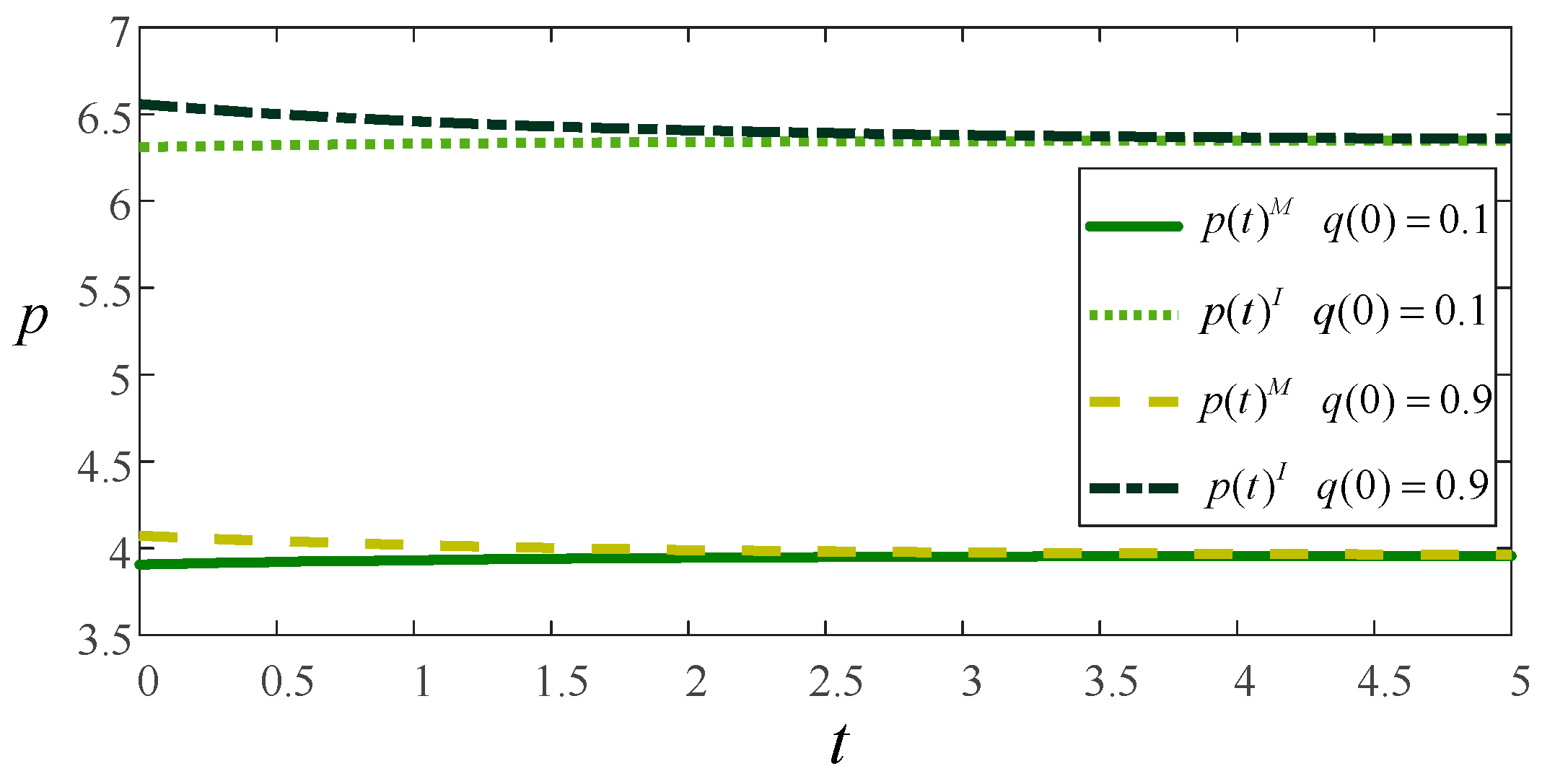
Figure 2 describes the evolutionary trajectory of product prices to make recommendations for long-term quality management as well as pricing behavior of firms. The figure illustrates that distinct price plans ought to be created for various product categories.
(i)
For innovative companies, particularly those offering products with initially high quality, a skimming pricing strategy is typically employed during the early stages of market entry. This involves setting a relatively high price to attract consumers seeking advanced features, high technological content, and innovative qualities—often referred to as early adopters or tech enthusiasts. After capturing a significant portion of the profit through this approach, the company gradually reduces prices to appeal to a broader consumer base, thereby increasing overall demand. For example, Tesla’s early supercar models, such as the Roadster, were priced above 500,000 yuan. By leveraging patents related to autonomous driving and click technology, Tesla attracted numerous users interested in technological innovation. However, as technological maturity and supply chain stability improve, Tesla has progressively introduced mid-to-high-end models aimed at the mass market.10
(ii)
For growing companies, particularly those whose initial product quality is not high, a penetration pricing strategy is typically employed. By setting low prices, these companies can rapidly capture market share and achieve substantial short-term profits. Such pricing also tends to attract pragmatic consumers who prioritize value. As sales extend over time and product performance diminishes, firms need to invest in technological improvements to attract additional customers. The costs incurred during this process can lead to an increase in product prices. For example, Lenovo adopted a similar marketing approach when introducing the Pentium-based computers into the Chinese market. Initially, they quickly gained market share through competitive pricing, establishing themselves as a leading player in China’s desktop computer industry at the time. Subsequently, through continuous technological innovation and R&D, they gradually launched more advanced product categories.11
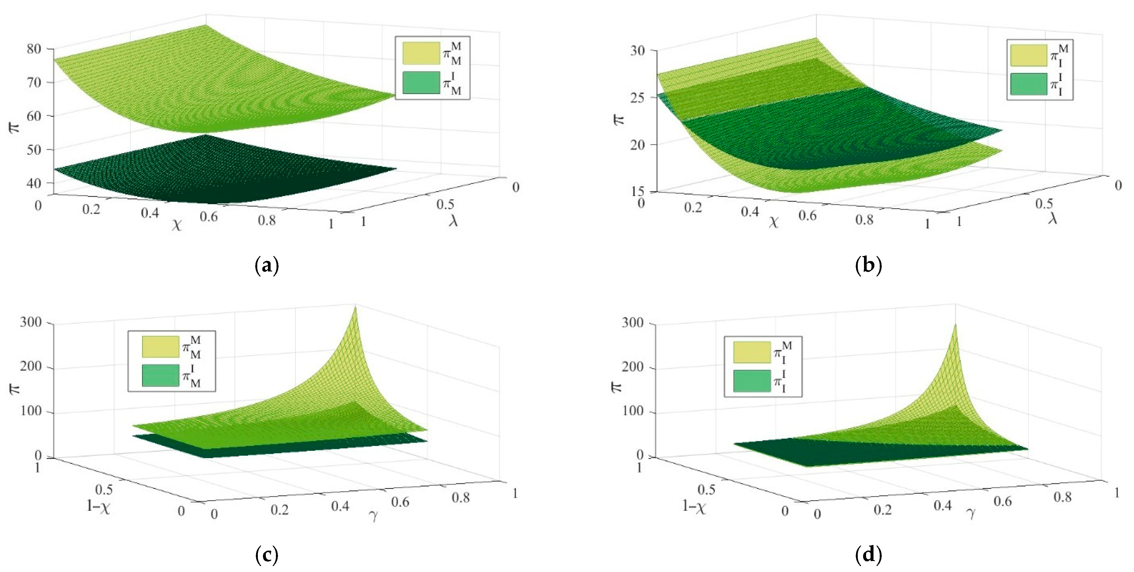
Figure 3 captures the impact of consumer segmentation based on quality preferences on the profits of the two model manufacturers and retail platforms. Figure 3a,b illustrate the effects of pragmatic consumers market share and quality sensitivity on profits. The earnings of manufacturers and retail platforms in both models exhibit a declining tendency as the market share of pragmatic consumer as well as quality sensitivity increases. Figure 3c,d show how innovative consumers’ market share and quality sensitivity affect profitability. As can be seen from the figures, innovative consumers market share and quality sensitivity positively affect profits.
The reason lies in the market size: an increase in the proportion of pragmatic consumers implies a decrease in the proportion of innovative consumers. Based on the demand functions of pragmatic and innovative consumers, under the same trade-in model and without considering market share fluctuations, the demand from innovative consumers will always exceed that of pragmatic consumers. When market share changes are taken into account, it becomes evident that the demand increase resulting from the rising market share of pragmatic consumers is less than the demand decrease among innovative consumers. Consequently, as the market share of pragmatic consumers grows, the overall market demand declines. Furthermore, the sensitivity of pragmatic consumers to quality and their market share negatively impact both sales prices and market performance. As this negative influence intensifies, sales prices tend to decrease further. Overall, these dynamics lead to a reduction in profits for manufacturers and retail platforms.
On the contrary, for the innovative consumer segment, an increase in market share signifies a rise in total demand. Additionally, the quality sensitivity of these consumers positively influences pricing, implying that both factors contribute to higher final profits. Specifically, the greater the market share held by innovative consumers and their heightened quality sensitivity, the more profit manufacturers and retail platforms can realize when offering trade-in options.
In conclusion, this study first segments consumers in the market into two types: pragmatic consumers and innovative consumers. It then examines the impact of this market segmentation on the profits of supply chain members, specifically within the context of trade-in environments. The analysis results reveal two key findings: first, a higher proportion of pragmatic consumers in the market; second, greater consumer sensitivity to product quality. Both of these factors ultimately lead to lower profits for both the manufacturer and the retail platform. Conversely, the presence of more innovative consumers tends to have the opposite effect.
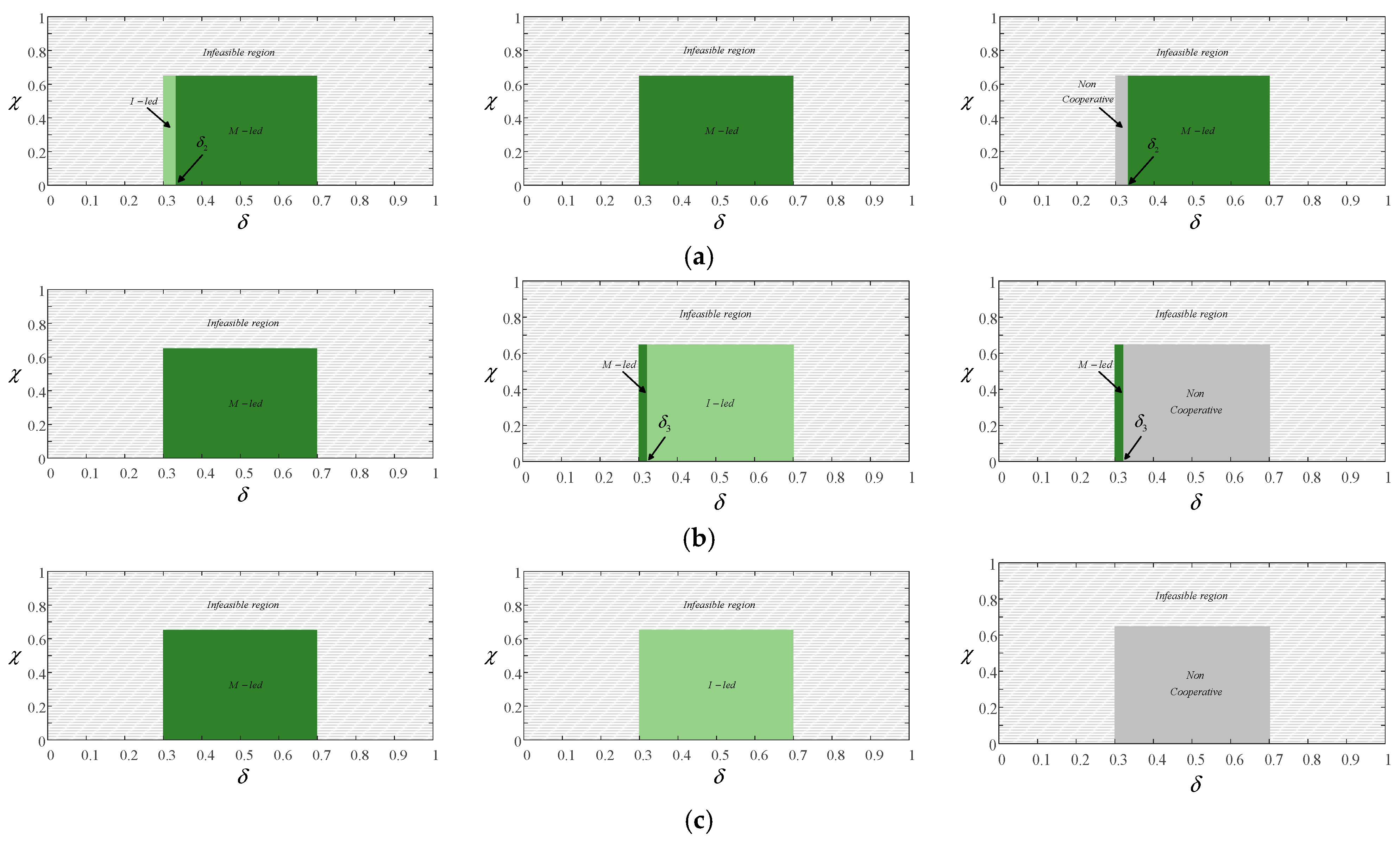
Figure 4 illustrates the selection of the trade-in model from different stakeholder perspectives. The choice of trade-in mode by the manufacturer and the retail platform is influenced by the product quality decay rate and the proportion of pragmatic consumers in the market. When the product quality decay rate is either too low or too high, or when the market share of pragmatic consumers is excessively large, it becomes unfeasible for supply chain members to participate in trade-in activities. Consequently, these regions are marked as infeasible zones and are excluded from the mode selection analysis. Considering economic benefits, within the feasible range where decision variables, state variables, demand, and profit are all positive, the manufacturer will always prefer to lead the trade-in process regardless of changes in the product quality depreciation rate and the market share of pragmatic consumers. Meanwhile, the platform tends to delegate the leading role in trade-in activities to the manufacturer when the product quality decay rate is low but opt to take the lead themselves when the depreciation rate is high.
Although the retail platform tends to set higher market prices during trade-in programs, and market demand is greater under the Model M. At this point, compared to the Model I, the scale economies achieved by the manufacturer in the Model M generate greater profit increases than the profit reductions caused by price effects. Consequently, the manufacturer will consistently prefer to lead the trade-in process themselves. For the platform, similarly, when the product quality decay rate is low, choosing manufacturer-led trade-in programs allows the retail platform to realize higher profits. Since the product quality decay rate negatively impacts quality investment, an increase in decay rate reduces quality improvement expenditures and associated costs. Coupled with p I > p M , this results in the retail platform favoring high prices and low costs during manufacturer-led trade-in programs. Under these conditions, adopting the Model I becomes more advantageous.
To ensure that both parties in the supply chain are willing to participate in the game, an optimal interval should be selected—one that satisfies both sides, meaning they will choose the same replacement policy led by either the manufacturer or the retailer. As illustrated in Figure 4c, in this context, when δ < δ 1 is at a certain level, both parties prefer the manufacturer-led replacement strategy. This choice aligns with their profit preferences, allowing both to achieve higher economic benefits and fostering a more long-term, stable partnership within the supply chain. Furthermore, as the product quality decay rate increases and the market share of pragmatic consumers expands, the region favoring manufacturer-led replacement strategies slightly enlarges. In other words, the more pragmatic consumers in the market, the more inclined the manufacturer and the retail platform are to favor manufacturer-led replacement policies. When the product quality decay rate exceeds a certain threshold, and considering profit-driven preferences, the parties’ choices become opposite, making cooperation unattainable.
Furthermore, considering social benefits, the overall social welfare generated by the manufacturer leading the trade-in programs consistently exceeds that of the retail platform leading such initiatives. From an environmental perspective, the same pattern holds true, with environmental benefits under the Model M always surpassing those under the Model M.
Based on this, within the feasible range defined by the product quality depreciation rate and the proportion of pragmatic consumers, manufacturers should proactively lead the trade-in process, leverage economies of scale and integrating end-to-end resources to maximize profits. Retail platforms, on the other hand, should dynamically switch between “leading” and “collaborative” roles based on the quality depreciation rate. When market demand causes the share of pragmatic consumers to surpass a certain threshold, initiatives such as enhancing trade-in campaigns and optimizing quality and cost structures are necessary. During periods when this group dominates the market, it is essential to emphasize the high cost-effectiveness of the manufacturer Model. Supply chain governance should prioritize consensus-driven leading strategies, establish shared benefit frameworks while consider social and environmental impacts. Additionally, companies must incorporate the product quality depreciation rate into core decision-making processes, develop predictive models, adopt recyclable designs in manufacturing, and coordinate with platforms to improve refurbishment systems, collectively expanding the feasible domain for trade-in activities.

7. Extension

7.1. Consideration of Government Subsidies

During the implementation of the trade-in program, governments often provide subsidies to incentivize providers to promote the initiative. For example, the Italian Chamber of Deputies’ Budget Committee introduced legislation that, from August to December 2020, increased subsidies for trade-in schemes targeting electric and hybrid vehicles. The subsidy costs were jointly borne by the Italian government and automobile dealers. Considering that these subsidies ultimately influence consumer behavior by offering discounts on trade-in, thereby affecting market demand, we include this factor in our analysis. We examine how varying discount rates offered by different trade-in scheme provider impacts mode selection.
This section is set up as follows: on the basis of the core model, the government grants a fixed subsidy S to the trade-in provider, and this trade-in provider offers price discounts to consumers participating in the trade-in activities. The same setting can be observed in Bai et al. (2021) [52]. The discount rates in the two models are η 1 and η 2 , respectively, and both of which are exogenous parameters of indeterminate size. By comparing the discount rates, we investigate the model selection problem of the trade-in provider in each of the three cases. (See Appendix A for detailed proof process).
Figure 5 presents the trade-in model choices of different subjects in three scenarios η 1 < η 2 η 1 = η 2 η 1 > η 2 , respectively. When η 1 < η 2 , i.e., the discount rate for manufacturer-led trade-in is smaller and the discount is larger, the manufacturer will choose to let the platform lead the trade-in when the product quality decay rate is low, and lead the trade-in itself when the product quality decay rate is high. Conversely, retail platform will decide to let the manufacturer drive the trade-in market. Considering the economic benefits, the two parties ultimately agree to cooperate in the area where the manufacturer leads the trade-in when the product quality decay rate is high. When the product quality decay rate is low, there is less negative impact on the price, when the market price of Model I is significantly higher than the market price of Model M. For manufacturer, choosing the Model I not only generates revenue from selling higher priced products, but also generates additional revenue by sharing the residual value of recycled products with the retail platform. However, as δ increases, the gap between p I and p M decreases, at which point the profit to be gained by choosing the Model I is very limited; conversely, making the manufacturer the trade-in leader not only enables it to receive the full net salvage value of the recovered product, but also the greater price discounts offered by the manufacturer lead to more demand. With the Model M, the manufacturer offers bigger price discounts, which allows the retail platform to earn more commissions on the sales volume.
When η 1 = η 2 , both supply chain members can offer the same trade-in discount. This situation is similar to our core model, and we will not go into too much detail here. When η 1 < η 2 , both parties are in a prisoner’s dilemma, and both will choose to dominate the trade-in themselves. Cooperation is not possible currently. The rationale is that the more price subsidies provided by the platform in the Model I, the stronger the promotion of demand, coupled with higher market prices, the Model I is the best choice for retail platform. Manufacturer may decide to take the lead in trade-in since it might be more profitable for them to offer consumers a reduced subsidy discount in the Model M and earn the difference between the government and consumer subsidies that way rather than opting for the Model I to increase demand.

7.2. Net Residual Value of Asymmetrically Recovered Products

We assume in the core model that the net residual value of recycled products in both the traditional trade-in models is equal. However, in practice, retail platforms typically delegate the intermediary recycling services in trade-in programs to third-party recyclers, incurring high commissioning fees that increase their costs beyond those of manufacturers conducting recycling independently. Consequently, manufacturers leading trade-in initiatives generally achieve higher net residual values for recycled products compared to retail platform-led programs. For example, JD.com outsources the intermediary service in its trade-in process to Aihuishou. In this section, we consider asymmetric net residual values of recycled products, denoting the residual value in manufacturer-led trade-in models as Δ 1 and that in retail platform-led models as Δ 2 ( Δ 1 > Δ 2 ) (See Appendix A for detailed proof process).
As can be seen from Figure 6, comparing the model choices in the core model, considering the net residual value of asymmetrically recovered products does not have a significant impact on the trade-in model choice. The main impact of this phenomenon is reflected in two aspects. First, it leads to a slight expansion of the scenario where the retail platform chooses to let the manufacturer take the lead in the trade-in service. Second, this slight expansion further increases the overall scope in which both supply chain participants—namely the manufacturer and the retail platform—eventually collaborate and opt for the manufacturer-led trade-in model. The net salvage value of the recycled product subsidizes the price of the product. With a larger net salvage value of the product recovered by the manufacturer, the manufacturer in the Model M will have the ability to set a lower market price to attract more consumers to buy the product, and its profit margin will be larger, and the region that chooses the manufacturer-led trade-in will naturally expand.

8. Conclusions and Management Insights

8.1. Conclusions

Although trade-in programs are regarded as an effective strategy to encourage consumers to return used products, increase the purchase frequency of new items, and generate additional revenue for businesses, manufacturers and retail platforms face the decision of whether to offer such services. Previous studies on trade-in schemes have not considered the process as a dynamic evolution nor accounted for consumer segmentation driven by heterogeneous product quality preferences. In our paper, we examine a supply chain composed of a manufacturer and a retail platform, where perceived product quality evolves over time according to certain patterns. Consumers are segmented into pragmatic and innovative types based on their perceptions and preferences for product quality. This study investigates the optimization problem of who should provide the trade-in service. Our goal is to reveal how consumer segmentation based on quality preferences influences supply chain members under two different models, describe the pricing relationships when the manufacturer or the retail platform offer trade-in services, and identify the conditions for achieving global optimality. We analyze scenarios where the trade-in service is managed by the manufacturer (Model M) and the retail platform (Model I), and through our analysis, we uncover the following key findings:
(i)
In the retail platform-led trade-in resale model, there is a double marginalization effect from the wholesale price to the retail price, which makes the market price of the product in the Model I constantly higher than that of the product in the Model M. The size of the quality improvement inputs in both models depends heavily on the net residual value of the recovered product.
(ii)
We observe that innovative companies tend to adopt a skimming pricing strategy, setting higher initial prices to attract early adopters. Subsequently, they gradually reduce quality and prices to appeal to more pragmatic consumers. In contrast, growing firms often employ penetration pricing by initially setting low prices to rapidly capture market share and attract pragmatic buyers. They then increase investment in quality improvements and raise market prices to attract more early adopters.
(iii)
Focus on the impact of consumer segmentation based on quality preferences on profitability. The results indicate that pragmatic consumers and innovative consumers have completely opposite effects on the profitability of manufacturers and platforms under both models. Specifically, the larger the market share of pragmatic consumers and the more sensitive they are to quality, the lower the profits manufacturers and retail platforms can achieve in the trade-in programs. Conversely, a higher market share of innovative consumers and greater sensitivity to quality enhance the profitability of supply chain members.
(iv)
Regarding the question of who should lead the trade-in program. From an economic efficiency perspective, the manufacturer generally prefers to take the lead in the trade-in process. The retail platform tends to delegate the trade-in authority to the manufacturer when product decay rates are low, whereas they prefer to control the trade-in process themselves when degradation rates are high. The equilibrium where both parties are satisfied occurs when the manufacturer leads the trade-in program under conditions of low product degradation. Considering social and environmental benefits, manufacturer-led trade-in initiatives consistently outperform retail platform-led programs.
(v)
Regarding the impact of consumer segmentation on the choice of the trade-in model, we find that the market share of different consumer types can significantly affect the selection of the trade-in approach. As the product decay rate increases, a higher proportion of pragmatic consumers in the market encourages the manufacturer and the retail platform to favor a manufacturer-led trade-in scheme.
(vi)
When considering the impact of government subsidies on the choice of the trade-in model, the manufacturer tends to lead the trade-in cooperation when their subsidy support is stronger and the product quality decay rate is high. When both parties receive equal subsidy support, they also prefer manufacturer-led trade-in arrangements when the product quality decay rate is low. However, if the retail platform’s subsidy support is greater, the supply chain members are unable to reach a cooperative agreement.
(vii)
Considering the impact of asymmetric net residual values of recovered products on the choice of the trade-in model, a higher net residual value for manufacturer-recovered products compared to retail platform-recovered products will lead both parties to favor a broader scope of manufacturer-led trade-in programs.

8.2. Management Insights

Our research provides valuable managerial insights for industry practitioners. Firstly, enterprises should base their decision-making on product quality degradation rates and the residual value of recovered goods. For durable products with low degradation rates and high residual value—such as premium home appliances and vehicles—a manufacturer-led approach should be prioritized, leveraging the manufacturer’s control over quality standards and pricing power to avoid retail platform double marginalization through markups. Additionally, manufacturers can generate extra residual value by independently handling the recycling process. Conversely, for fast-moving consumer electronics with rapid quality decline and low residual value—such as smartphones—retail platforms can take the lead, utilizing their proximity to consumers to streamline recycling procedures and increase participation rates, while manufacturers focus on improving product quality. Secondly, to serve pragmatic consumers, it is essential to emphasize a combination of “cost savings plus functional reassurance,” employing a “high depreciation + fixed subsidy” model, supported by transparent valuation tools and convenient recycling services to alleviate concerns over pricing and functionality. For innovative consumers, highlight “technological upgrades plus experience enhancement” by offering “low base depreciation plus innovative subsidies,” coupled with product trials and offline demonstrations, to satisfy their desire for novelty and improve conversion efficiency. Finally, attention should be given to government subsidy policies. If subsidies favor manufacturers, discounts should be increased to reinforce their dominant position. If subsidies favor retail platforms, profit-sharing arrangements can mitigate the prisoner’s dilemma. Additionally, leveraging manufacturers’ recycling technology advantages—especially in asymmetric residual value scenarios where manufacturers retain higher residual values—can expand the applicability of manufacturer-led models, particularly in lower-tier markets, by utilizing proprietary networks to enhance trade-in coverage and profitability.
It is worth noting that our research has certain limitations that warrant further investigation in the future. Firstly, our study assumes that the old-for-new supply chain consists of a single manufacturer and a retail platform; however, in reality, multiple manufacturers and retail platforms often offer trade-in services for the same product. Therefore, examining the competition among multiple supply chain members is highly necessary. Secondly, we did not consider the risk preferences of supply chain participants involved in the trade-in process; future research could explore their risk sensitivities and related factors [54,55]. Thirdly, the recycling process in a trade-in supply chain typically involves third-party recycling platforms dedicated to collecting used products. Future studies could analyze how the participation of third-party recycling platforms influences the selection of providers in the trade-in scheme. Fourth, when considering consumer segmentation, we have solely focused on consumer quality preferences and have not accounted for the impact of environmental consciousness. However, environmental awareness plays a significant role in the decision-making process regarding participation in trade-in programs. Future analyses should incorporate this factor. Lastly, as a means to reduce electronic waste, the trade-in approach plays a crucial role in building an environmentally friendly society. From an environmental benefits perspective, research could focus on identifying which entities are most advantageous in providing trade-in services to promote green and sustainable development.

Author Contributions

Writing—review & editing, D.M. and J.H.; Writing—original draft, D.H.; Formal analysis, D.M.; Methodology, D.M.; Data curation, D.H.; Supervision, J.H. All authors have read and agreed to the published version of the manuscript.

Funding

This work was supported by the National Natural Science Foundation of China (72202113; 72474112), Natural Science Foundation of Shandong Province (ZR2022QG017; ZR2023MG063) and Project of Youth Innovation and Technology Support Program for Higher Education Institutions in Shandong Province (2024KJL002).

Data Availability Statement

Dataset available on request from the authors.

Conflicts of Interest

The authors declare no conflicts of interest regarding the publication of this paper.

Abbreviations

The following abbreviations are used in this manuscript:
M-ledManufacturer offer trade-in service
I-ledRetail platform offer trade-in service

Appendix A

Proof of Proposition 1.
The differential game model for Model M is modeled as follows:
max u ( ) ; p ( ) J M M = 0 + e r t ( 1 φ ) p ( t ) + Δ ( D R + D N ) 1 2 k u 2 ( t ) d t J I M = 0 + e r t φ p ( t ) ( D R + D N ) d t s . t . q ˙ ( t ) = u ( t ) δ q ( t )   ,   q ( 0 ) = q 0
We use inverse induction to show that, according to Bellman’s theory of continuous-type dynamic programming, for any state, there exists a continuously differentiable function, which satisfies the following Hamilton–Jacobi-Bellman (abbreviated as HJB) equation:
r V I M = max φ p a + [ ( 1 χ ) γ χ λ δ ] q β p + V I M ( u δ q )
where V I M   is the optimal value function of the retail platform under Model M, V I M represents the profit of the retail platform in the whole operation plan period, and B is the first-order derivative of the optimal value function of the retail platform with respect to the perceived quality of the product, which represents the impact of the unit change in the perceived quality of the product on the profit of the retail platform. The HJB equation of the retail platform under the Model M shown in Equation (A2) indicates that the retail platform will not only consider the immediate profit, but also consider the impact of the decision on the dynamic change in the perceived quality of the product and its impact on the long-term interests of the enterprise when making the decision, therefore, the optimal decision is a far-sighted decision that considers the immediate interests of the enterprise and the long-term interests of the enterprise that are affected by the perceived quality of the product. Considering that the model is a differential game problem with infinite planning horizon, for the sake of notational simplicity, the following solution procedure omits the time variable t . In the Model M, the retail platform does not make any decisions on the quality of their products. In Model M, the retail platform does not make decisions, so there is no reaction function. Next, the manufacturer’s HJB equation is constructed:
r V M M = max u ; p [ ( 1 φ ) p + Δ ] a + [ ( 1 χ ) γ χ λ δ ] q β p 1 2 k u 2 + V M M ( u δ q )
where V M M   is the manufacturer’s optimal value function under Model M, and V M M is the first-order derivative of the manufacturer’s optimal value function with respect to the perceived quality of the product, reflecting the impact of a unit change in the perceived quality of the product on the manufacturer’s profit. Equation (A3) also reflects the manufacturer’s decision to take into account both immediate benefits and long-term benefits under the influence of environmental goodwill. Based on the first-order optimality conditions at the right-hand end of the middle equation of Equation (A3), the optimal decision for the manufacturer’s quality-improvement inputs and retail price can be obtained as follows:
u = V M M k p = ( 1 φ ) a Δ β 2 ( 1 φ ) β + ( 1 χ ) γ χ λ δ 2 β q
It can be found that the manufacturer’s optimal decisions are all functions of the perceived quality of the product, which reflects the manufacturer’s visionary decisions based on the perceived quality of the product. Substituting Equation (A4) into the HJB equations for the manufacturer and the platform, the following set of HJB equations is obtained:
r V M M = ( 1 φ ) a + Δ β + ( 1 φ ) ( 1 χ ) γ χ λ δ q 2 4 ( 1 φ ) β 1 2 k u 2 + V M M ( u δ q ) + ( V M M ) 2 2 k δ V M M q r V I M = φ ( 1 φ ) ( 1 χ ) q γ χ λ δ q + a Δ β Δ β + ( 1 φ ) ( 1 χ ) γ q χ λ δ q + a 4 ( 1 φ ) 2 β + V I M ( V M M k δ q )
Based on the relationship between the value functions at the left and right ends of Equation (A5) and the perceived quality of the product, it is assumed that the optimal value functions of the manufacturer and the platform, respectively, satisfy the following relationship:
V M M = A 1 M q 2 + A 2 M q + A 3 M , V M M = 2 A 1 M q + A 2 M V I M = B 1 M q 2 + B 2 M q + B 3 M , V I M = 2 B 1 M q + B 2 M
where A I M , B i M , i 1 , 2 , 3 denote the coefficients to be determined for the optimal value functions of the manufacturer and the retail platform, respectively, and i is a constant. Substituting Equation (A6) into the HJB system of Equation (A5), the constant relationship can be obtained as follows:
r A 1 M q 2 + A 2 M q + A 3 M ( 1 φ ) a + Δ β + ( 1 φ ) ( 1 χ ) γ χ λ δ q 2 4 ( 1 φ ) β + 4 ( A 1 M ) 2 q 2 + 4 A 1 M A 2 M q + ( A 2 M ) 2 2 k 2 A 1 M q + A 2 M δ q r B 1 M q 2 + B 2 M q + B 3 M φ ( 1 φ ) a + ( 1 φ ) ( 1 χ ) γ χ λ δ q 2 Δ 2 β 2 4 ( 1 φ ) 2 β + 2 B 1 M q + B 2 M 2 A 1 M δ k q + A 2 M k
Based on the left and right ends of Equation (A7) as a function of the perceived quality of the product, the following specific expressions for the constant coefficients to be determined can be obtained:
A 1 M = k r + 2 δ k r + 2 δ 2 2 1 φ ( 1 χ ) γ χ λ δ 2 k β 4 A 2 M = ( 1 φ ) a + Δ β ( 1 χ ) γ χ λ δ β r + r + 2 δ 2 2 1 φ ( 1 χ ) γ χ λ δ 2 k β A 3 M = ( 1 φ ) a + Δ β 2 4 ( 1 φ ) r β + ( A 2 M ) 2 2 r k B 1 M = k φ ( 1 χ ) γ χ λ δ 2 4 β r k 4 A 1 M + 2 δ k B 2 M = k a φ ( 1 χ ) γ χ λ δ 2 β r k 2 A 1 M + δ k + 2 B 1 M A 2 M r k 2 A 1 M + δ k B 3 M = φ ( 1 φ ) 2 a 2 Δ β 2 4 r ( 1 φ ) 2 β + A 2 M B 2 M r k
To further obtain the time trajectory of product perceived quality, Equation (A8) is substituted into Equation (A4) to obtain the expression about the relevant decision, and further substituted into the kinetic equation of product perceived quality to obtain the first order differential equation of product perceived quality as follows:
d q ( t ) d t = ( 1 φ ) a + Δ β ( 1 χ ) γ χ λ δ k β r + r + 2 δ 2 2 1 φ ( 1 χ ) γ χ λ δ 2 k β r + 2 δ 2 2 1 φ ( 1 χ ) γ χ λ δ 2 k β r 2 q ( t ) q ( t ) = q 0
Solving Equation (A9) yields the optimal time path for the perceived quality of the product under Model M:
q ( t ) = e r + 2 δ 2 2 1 φ ( 1 χ ) γ χ λ δ 2 k β r t 2 q 0 q M + q M
where q M = 2 ( 1 φ ) a + Δ β ( 1 χ ) γ χ λ δ 4 r δ + 4 δ 2 k β 2 1 φ ( 1 χ ) γ χ λ δ 2 denotes the steady state of perceived product quality in the M-mode, and substituting (A10) into (A6) yields the optimal decisions of the manufacturer and retail platform:
u M = 2 δ ( 1 φ ) a + Δ β ( 1 χ ) γ χ λ δ 4 r δ + 4 δ 2 k β 2 1 φ ( 1 χ ) γ χ λ δ 2 p M = k 4 r δ + 4 δ 2 ( 1 φ ) a Δ β + 4 Δ ( 1 φ ) ( 1 χ ) γ χ λ δ 2 2 ( 1 φ ) 4 r δ + 4 δ 2 k β 2 1 φ ( 1 χ ) γ χ λ δ 2
Bringing Equation (A11) into (A1) gives the market demand at this point as:
D M = k β a ( 1 φ ) + Δ β 4 r δ + 4 δ 2 2 ( 1 φ ) 4 r δ + 4 δ 2 k β 2 1 φ ( 1 χ ) γ χ λ δ 2
When demand is 0, solve for the highest consumer willingness to pay as:
p M = 4 r δ + 4 δ 2 a k + 2 Δ ( 1 χ ) γ χ λ δ 2 4 r δ + 4 δ 2 k β 2 1 φ ( 1 χ ) γ χ λ δ 2
Consumer surplus and social welfare at this point are:
C S M = D M p M p M 2 r = k 2 β ( 1 φ ) a + Δ β 2 4 r δ + 4 δ 2 2 4 r ( 1 φ ) 2 4 r δ + 4 δ 2 k β 2 1 φ ( 1 χ ) γ χ λ δ 2 2 S W M = C S M + V M M + V I M
Proposition 1 is proved. □
Proof of Proposition 2.
The differential game model for Model I is modeled as follows:
max w ( ) , u ( ) J M I = 0 + e r t w ( t ) + τ Δ ( D R + D N ) 1 2 k u 2 ( t ) d t max p ( ) J I I = 0 + e r t p ( t ) w ( t ) + 1 τ Δ ( D R + D N ) d t s . t . q ˙ ( t ) = u ( t ) δ q ( t ) , q ( 0 ) = q 0
We use the inverse induction method, which requires us to first solve for the response decision of the retail platform. According to Bellman’s continuous dynamic programming theory, for any state q ( t ) 0 , there exists a continuously differentiable function V I I   that satisfies the following Hamilton–Jacobi-Bellman (abbreviated as HJB) equation:
r V I I = max p p w + 1 τ Δ a + ( 1 χ ) γ χ λ δ q β p + V I I u δ q
where V I I   is the optimal value function of the retail platform under Model I, which represents the profit of the retail platform in the whole operation plan period, and V I I   is the first-order derivative of the optimal value function of the retail platform with respect to the perceived quality of the product, which represents the impact of the change in the perceived quality unit of the product on the profit of the retail platform. The HJB equation of the retail platform under Model I shown in Equation (A13) indicates that the retail platform will not only consider the immediate profit, but also consider the impact of the decision on the dynamic change in the perceived quality of the product and its impact on the long-term interests of the enterprise when making the decision, therefore, the optimal decision is a far-sighted decision that considers the immediate interests of the enterprise and the long-term interests of the enterprise that are affected by the perceived quality of the product. Considering that the model is a differential game problem with infinite planning period, the time variable t is omitted in the following solution process for the sake of notational simplicity. According to the first-order optimality condition at the right end of Equation (A16), the response function for the retail platform decision can be obtained as follows:
p = a 1 τ Δ w β 2 β + ( 1 χ ) γ χ λ δ 2 β q
Equation (A17) is further substituted into the manufacturer’s goal function to obtain the manufacturer’s HJB equation according to Bellman’s continuous dynamic programming method as follows:
r V M I = max w ; u a + ( 1 χ ) γ χ λ δ q + 1 τ Δ w β 2 w + τ Δ 1 2 k u 2 + V M I u δ q
where V M I is the manufacturer’s optimal value function under Model I, and V M I is the first-order derivative of the manufacturer’s optimal value function with respect to the perceived quality of the product, which reflects the impact of a unit change in the perceived quality of the product on the manufacturer’s profit. Equation (A18) also reflects the manufacturer’s decision to consider both immediate benefits and long-term benefits under the influence of environmental goodwill. Based on the first-order optimality conditions at the right-hand end of the middle equation of Equation (A18), the optimal decision for the manufacturer’s quality improvement inputs and wholesale price can be obtained as follows:
u = V M I k w = a + 1 2 τ Δ β 2 β + ( 1 χ ) γ χ λ δ 2 β q
It can be found that the manufacturer’s optimal decisions are all functions of the perceived quality of the product, which reflects the manufacturer’s far-sighted decisions based on the perceived quality of the product. Substituting Equation (A19) into the response function (A17) of the platform strategy, the retail price decision of the platform is obtained as:
p = 3 a Δ β 4 β + 3 ( 1 χ ) γ χ λ δ 4 β q
Similarly, from Equation (A20), the optimal strategy of the retail platform is also a function of the perceived quality of the product, i.e., the retail platform bases its far-sighted pricing decision on the feedback of the perceived quality of the product. To further obtain the optimal value functions of the manufacturer and the retail platform as well as the specific expressions for the perceived quality of the product, Equations (A19) and (A20) are substituted into the HJB equations of the manufacturer and the platform, respectively, to obtain the following set of HJB equations:
r V M I = a + Δ β + ( 1 χ ) γ χ λ δ q 2 8 β + V M I 2 2 k V M I δ q r V I I = a + Δ β + ( 1 χ ) γ χ λ δ q 2 16 β + V I I V M I k δ q
Based on the relationship between the value functions at the left and right ends of Equation (A21) and the perceived quality of the product, it is assumed that the optimal value functions of the manufacturer and the platform, respectively, satisfy the following relationship:
V M I = A 1 I q 2 + A 2 I q + A 3 I ,   V M I = 2 A 1 I q + A 2 I V I I = B 1 I q 2 + B 2 I q + B 3 I ,   V I I = 2 B 1 I q + B 2 I
where A I I , B i I , i 1 , 2 , 3 denote the coefficients to be determined for the optimal value functions of the manufacturer and the retail platform, respectively, and i is a constant. Substituting Equation (A22) into the HJB system of Equations (A21), the constant relationship can be obtained as follows:
r A 1 I q 2 + A 2 I q + A 3 I a + Δ β + ( 1 χ ) γ χ λ δ q 2 8 β + 4 A 1 I 2 q 2 + 4 A 1 I A 2 I q + A 2 I 2 2 k 2 A 1 I q + A 2 I δ q r B 1 I q 2 + B 2 I q + B 3 I a + Δ β + ( 1 χ ) γ χ λ δ q 2 16 β + 2 B 1 I q + B 2 I 2 A 1 I k δ q k + A 2 I k
Based on the left and right ends of Equation (A23) as a function of the perceived mass of the product, the following specific expression for the constant coefficient to be determined is obtained:
A 1 I = k r + 2 δ k r + 2 δ 2 ( 1 χ ) γ χ λ δ 2 k β 4 A 2 I = a + β Δ ( 1 χ ) γ χ λ δ 2 β r + r + 2 δ 2 ( 1 χ ) γ χ λ δ 2 k β A 3 I = a + β Δ 2 8 r β + A 2 I 2 2 r k B 1 I = k ( 1 χ ) γ χ λ δ 2 16 β r k 4 A 1 I + 2 k δ B 2 I = 2 k a + Δ β ( 1 χ ) γ χ λ δ 16 β r k 2 A 1 I + k δ + 2 B 1 I A 2 I r k 2 A 1 I + k δ B 3 I = a + Δ β 2 16 r β + A 2 I B 2 I r k
To further obtain the time trajectory of the perceived quality of the product, Equation (A24) is substituted into Equation (A19) to obtain the expression about the relevant decision and further substituted into the kinetic equation of the perceived quality of the product to obtain the first order differential equation of the perceived quality of the product as follows:
d q ( t ) d t = a + β Δ ( 1 χ ) γ χ λ δ 2 k β r + r + 2 δ 2 ( 1 χ ) γ χ λ δ 2 k β r + 2 δ 2 ( 1 χ ) γ χ λ δ 2 k β r 2 q ( t )   q ( t ) = q 0
Solving Equation (A25) yields the optimal time path for the perceived quality of the product under Model I:
q ( t ) = e r + 2 δ 2 ( 1 χ ) γ χ λ δ 2 k β r t 2 q 0 q I + q I
where q I = a + β Δ ( 1 χ ) γ χ λ δ 4 r δ + 4 δ 2 k β ( 1 χ ) γ χ λ δ 2 denotes the steady state of perceived product quality in Model I. Substituting (A26) into (A19) and (A20) yields the optimal decisions of the manufacturer and the retail platform:
u I = δ a + β Δ ( 1 χ ) γ χ λ δ 4 r δ + 4 δ 2 k β ( 1 χ ) γ χ λ δ 2 w I = k 4 r δ + 4 δ 2 a + 1 τ Δ β + 2 τ Δ ( 1 χ ) γ χ λ δ 2 2 4 r δ + 4 δ 2 k β ( 1 χ ) γ χ λ δ 2 p I = k 4 r δ + 4 δ 2 3 a Δ β + 4 Δ ( 1 χ ) γ χ λ δ 2 4 4 r δ + 4 δ 2 k β ( 1 χ ) γ χ λ δ 2
Bringing (A27) into (A15) gives the market demand at this point:
D I = k β a + Δ β 4 r δ + 4 δ 2 4 4 r δ + 4 δ 2 k β ( 1 χ ) γ χ λ δ 2
Solve for the highest consumer willingness to pay when demand is 0:
p I = 4 r δ + 4 δ 2 a k + Δ ( 1 χ ) γ χ λ δ 2 4 r δ + 4 δ 2 k β ( 1 χ ) γ χ λ δ 2
Consumer surplus and social welfare at this point are:
C S I = D I p I p I 2 r = k 2 β a + Δ β 2 4 r δ + 4 δ 2 2 32 r 4 r δ + 4 δ 2 k β ( 1 χ ) γ χ λ δ 2 2 S W I = C S I + V M I + V I I
Proposition 2 is proved. □
Proof of Proposition 3.
q M q I = ( 1 χ ) γ χ λ δ ( 1 2 φ ) 4 r δ + 4 δ 2 a k β + Δ β 4 r δ + 4 δ 2 k β 2 φ ( 1 χ ) γ χ λ δ 2 4 r δ + 4 δ 2 k β 2 1 φ ( 1 χ ) γ χ λ δ 2 4 r δ + 4 δ 2 k β ( 1 χ ) γ χ λ δ 2
Known that ( 1 χ ) γ χ λ δ > 0 ,   4 r δ + 4 δ 2 k β 2 1 φ ( 1 χ ) γ χ λ δ 2 4 r δ + 4 δ 2 k β ( 1 χ ) γ χ λ δ 2 > 0 ,
if ( 1 2 φ ) 4 r δ + 4 δ 2 a k β + Δ β 4 r δ + 4 δ 2 k β 2 φ ( 1 χ ) γ χ λ δ 2 > 0 ,
that is Δ > ( 2 φ 1 ) 4 r δ + 4 δ 2 a k 4 r δ + 4 δ 2 k β 2 φ ( 1 χ ) γ χ λ δ 2 , then q M > q I .
And if ( 1 2 φ ) 4 r δ + 4 δ 2 a k β + Δ β 4 r δ + 4 δ 2 k β 2 φ ( 1 χ ) γ χ λ δ 2 < 0 ,
that is 0 < Δ < ( 2 φ 1 ) 4 r δ + 4 δ 2 a k 4 r δ + 4 δ 2 k β 2 φ ( 1 χ ) γ χ λ δ 2 , then q M < q I .
u M u I = δ ( q M q I )
Since   δ > 0 , the comparison is the same as q M vs. q I .
p M p I = 8 Δ φ 1 φ ( 1 χ ) γ χ λ δ 4 k 2 β ( 1 φ ) a + ( 1 + φ ) Δ β 4 r δ + 4 δ 2 2 + 6 4 φ Δ β 2 ( 1 φ ) a + 2 1 φ 2 3 a Δ β ( 1 χ ) γ χ λ δ 2 4 r δ + 4 δ 2 k 4 ( 1 φ ) 4 r δ + 4 δ 2 k β 2 1 φ ( 1 χ ) γ χ λ δ 2 4 r δ + 4 δ 2 k β ( 1 χ ) γ χ λ δ 2
Known that 4 ( 1 φ ) 4 r δ + 4 δ 2 k β 2 1 φ ( 1 χ ) γ χ λ δ 2 4 r δ + 4 δ 2 k β ( 1 χ ) γ χ λ δ 2 > 0 , and 8 Δ φ 1 φ ( 1 χ ) γ χ λ δ 4 k 2 β ( 1 φ ) a + ( 1 + φ ) Δ β 4 r δ + 4 δ 2 2 + 6 4 φ Δ β 2 ( 1 φ ) a + 2 1 φ 2 3 a Δ β ( 1 χ ) γ χ λ δ 2 4 r δ + 4 δ 2 k < 0
then p M < p I .
Proposition 3 is proved. □
Proof of Proposition 4.
D M D I = 2 k β 4 r δ + 4 δ 2 a ( 1 φ ) 7 4 r δ + 4 δ 2 k β + 2 1 φ 8 ( 1 χ ) γ χ λ δ 2 + Δ β 8 ( 1 φ ) 4 r δ + 4 δ 2 k β + 2 1 φ 2 8 ( 1 χ ) γ χ λ δ 2 8 ( 1 φ ) 4 r δ + 4 δ 2 k β 2 1 φ ( 1 χ ) γ χ λ δ 2 4 r δ + 4 δ 2 k β ( 1 χ ) γ χ λ δ 2
Known that 8 ( 1 φ ) 4 r δ + 4 δ 2 k β 2 1 φ ( 1 χ ) γ χ λ δ 2 4 r δ + 4 δ 2 k β ( 1 χ ) γ χ λ δ 2 > 0 , and 2 k β 4 r δ + 4 δ 2 a ( 1 φ ) 7 4 r δ + 4 δ 2 k β + 2 1 φ 8 ( 1 χ ) γ χ λ δ 2 + Δ β 8 ( 1 φ ) 4 r δ + 4 δ 2 k β + 2 1 φ 2 8 ( 1 χ ) γ χ λ δ 2 > 0 ,
then D M > D I .
D R M D R I = 4 ( 1 φ ) a + Δ β ( 4 r δ + 4 δ 2 ) k β ( 1 χ ) γ χ λ δ 2 * ( 4 r δ + 4 δ 2 ) k β 4 ( 1 φ ) ( 1 χ ) γ χ λ δ 2 4 ( 1 φ ) λ δ ( 1 χ ) γ χ λ δ 2 ( 1 φ ) ( a + Δ β ) ( 4 r δ + 4 δ 2 ) k β 2 ( 1 φ ) ( 1 χ ) γ χ λ δ 2 * k β ( 4 r δ + 4 δ 2 ) 4 λ δ ( 1 χ ) γ χ λ δ 4 ( 1 χ ) γ χ λ δ 2 8 ( 1 φ ) ( 4 r δ + 4 δ 2 ) k β 2 ( 1 φ ) ( 1 χ ) γ χ λ δ 2 ( 4 r δ + 4 δ 2 ) k β ( 1 χ ) γ χ λ δ 2
Known that 8 ( 1 φ ) 4 r δ + 4 δ 2 k β 2 1 φ ( 1 χ ) γ χ λ δ 2 4 r δ + 4 δ 2 k β ( 1 χ ) γ χ λ δ 2 > 0 ,
if 4 ( 1 φ ) a + Δ β 4 r δ + 4 δ 2 k β ( 1 χ ) γ χ λ δ 2 2 ( 1 φ ) a + Δ β 4 r δ + 4 δ 2 k β 2 1 φ ( 1 χ ) γ χ λ δ 2 4 r δ + 4 δ 2 k β 4 1 φ ( 1 χ ) γ χ λ δ ( 1 χ ) γ χ λ δ + λ δ > 0 ,
that is Δ > Ω 1 ,
Ω 1 = a ( 1 φ ) 4 r δ + 4 δ 2 k β 2 1 φ ( 1 χ ) γ χ λ δ 2 4 r δ + 4 δ 2 k β 4 ( 1 χ ) γ χ λ δ ( 1 χ ) γ χ λ δ + λ δ 2 4 r δ + 4 δ 2 k β ( 1 χ ) γ χ λ δ 2 4 r δ + 4 δ 2 k β 4 1 φ ( 1 χ ) γ χ λ δ ( 1 χ ) γ χ λ δ + λ δ β 2 4 r δ + 4 δ 2 k β ( 1 χ ) γ χ λ δ 2 4 r δ + 4 δ 2 k β 4 1 φ ( 1 χ ) γ χ λ δ ( 1 χ ) γ χ λ δ + λ δ ( 1 φ ) 4 r δ + 4 δ 2 k β 2 1 φ ( 1 χ ) γ χ λ δ 2 4 r δ + 4 δ 2 k β 4 ( 1 χ ) γ χ λ δ ( 1 χ ) γ χ λ δ + λ δ
then D R M > D R I .
And if
16 ( 1 φ ) a + Δ β 4 ( r δ + δ 2 ) k β ( 1 χ ) γ χ λ δ 2 ( r δ + δ 2 ) k β ( 1 φ ) ( 1 χ ) γ + λ δ ( 1 χ ) ( 1 χ ) γ χ λ δ 8 ( 1 φ ) a + Δ β 4 ( r δ + δ 2 ) k β 2 ( 1 φ ) ( 1 χ ) γ χ λ δ 2 ( r δ + δ 2 ) k β ( 1 χ ) γ + λ δ ( 1 χ ) ( 1 χ ) γ χ λ δ < 0
that is 0 < Δ <   Ω 1 , then D R M < D R I .
D N M D N I = 4 a ( 1 φ ) + Δ β ( 4 r δ + 4 δ 2 ) k β + 4 ( 1 φ ) ( 1 χ ) γ χ λ δ ( χ γ + χ λ δ ) * ( 4 r δ + 4 δ 2 ) k β ( 1 χ ) γ χ λ δ 2 2 ( 1 φ ) ( a + Δ β ) ( 4 r δ + 4 δ 2 ) k β 2 ( 1 φ ) ( 1 χ ) γ χ λ δ 2 * ( 4 r δ + 4 δ 2 ) k β + 4 ( 1 φ ) ( 1 χ ) γ χ λ δ ( χ γ + χ λ δ ) 2 ( 1 φ ) 4 r δ + 4 δ 2 k β 2 1 φ ( 1 χ ) γ χ λ δ 2 4 4 r δ + 4 δ 2 k β ( 1 χ ) γ χ λ δ 2
Known that 2 ( 1 φ ) 4 r δ + 4 δ 2 k β 2 1 φ ( 1 χ ) γ χ λ δ 2 4 4 r δ + 4 δ 2 k β ( 1 χ ) γ χ λ δ 2 > 0 ,
if 4 a ( 1 φ ) + Δ β 4 r δ + 4 δ 2 k β 4 ( 1 φ ) ( 1 χ ) γ χ λ δ 2 + 4 ( 1 φ ) γ ( 1 χ ) γ χ λ δ 4 r δ + 4 δ 2 k β ( 1 χ ) γ χ λ δ 2 2 ( 1 φ ) a + Δ β 4 r δ + 4 δ 2 k β 2 1 φ ( 1 χ ) γ χ λ δ 2 k β 4 r δ + 4 δ 2 + 4 γ ( 1 χ ) γ χ λ δ 4 ( 1 χ ) γ χ λ δ 2 > 0 ,
that is Δ > Ω 2 ,
Ω 2 = 2 a ( 1 φ ) 4 r δ + 4 δ 2 k β 2 1 φ ( 1 χ ) γ χ λ δ 2 k β 4 r δ + 4 δ 2 + 4 γ ( 1 χ ) γ χ λ δ 4 ( 1 χ ) γ χ λ δ 2 4 a ( 1 φ ) 4 r δ + 4 δ 2 k β ( 1 χ ) γ χ λ δ 2 4 r δ + 4 δ 2 k β 4 ( 1 φ ) ( 1 χ ) γ χ λ δ 2 + 4 ( 1 φ ) γ ( 1 χ ) γ χ λ δ β 4 4 r δ + 4 δ 2 k β ( 1 χ ) γ χ λ δ 2 4 r δ + 4 δ 2 k β 4 ( 1 φ ) ( 1 χ ) γ χ λ δ 2 + 4 ( 1 φ ) γ ( 1 χ ) γ χ λ δ 2 ( 1 φ ) 4 r δ + 4 δ 2 k β 2 1 φ ( 1 χ ) γ χ λ δ 2 k β 4 r δ + 4 δ 2 + 4 γ ( 1 χ ) γ χ λ δ 4 ( 1 χ ) γ χ λ δ 2
then D N M > D N I .
And if 4 a ( 1 φ ) + Δ β 4 r δ + 4 δ 2 k β 4 ( 1 φ ) ( 1 χ ) γ χ λ δ 2 + 4 ( 1 φ ) γ ( 1 χ ) γ χ λ δ 4 r δ + 4 δ 2 k β ( 1 χ ) γ χ λ δ 2 2 ( 1 φ ) a + Δ β 4 r δ + 4 δ 2 k β 2 1 φ ( 1 χ ) γ χ λ δ 2 k β 4 r δ + 4 δ 2 + 4 γ ( 1 χ ) γ χ λ δ 4 ( 1 χ ) γ χ λ δ 2 < 0 ,
that is 0 < Δ <   Ω 2 , then D N M < D N I .
Proposition 4 is proved. □
Proof of Extended Model 7.1.
In Model M, the demand functions for the pragmatic consumer and the innovative consumer are as follows:
D R M = χ a λ δ q ( t ) β η 1 p ( t ) ;   D N M = ( 1 χ ) a + γ q ( t ) β η 1 p ( t )
In Model I, the demand functions for the pragmatic consumer and the innovative consumer are as follows:
D R I = χ a λ δ q ( t ) β η 2 p ( t ) ; D N I = ( 1 χ ) a + γ q ( t ) β η 2 p ( t )
The differential game model for Model M is modeled as follows:
max u ( ) ; p ( ) J M M = 0 + e r t ( 1 φ ) p ( t ) + Δ ( D R + D N ) 1 2 k u 2 ( t ) + S d t   J I M = 0 + e r t φ p ( t ) ( D R + D N ) d t s . t . q ˙ ( t ) = u ( t ) δ q ( t ) ,   q ( 0 ) = q 0
The differential game model for Model I is modeled as follows:
max w ( ) , u ( ) J M I = 0 + e r t w ( t ) + τ Δ ( D R + D N ) 1 2 k u 2 ( t ) + S d t max p ( ) J I I = 0 + e r t p ( t ) w ( t ) + 1 τ Δ ( D R + D N ) d t s . t . q ˙ ( t ) = u ( t ) δ q ( t ) ,   q ( 0 ) = q 0
The proof of the extended model is similar to the core model.
The equilibrium results of model M are as follows:
q M = 2 ( 1 φ ) a + η 1 Δ β ( 1 χ ) γ χ λ δ k η 1 β 4 r δ + 4 δ 2 2 ( 1 φ ) ( 1 χ ) γ χ λ δ 2 u M = 2 δ ( 1 φ ) a + η 1 Δ β ( 1 χ ) γ χ λ δ k η 1 β 4 r δ + 4 δ 2 2 ( 1 φ ) ( 1 χ ) γ χ λ δ 2 p M = ( 1 φ ) a Δ β 4 r δ + 4 δ 2 k η 1 + 2 ( 1 φ ) η 1 + 1 Δ ( 1 χ ) γ χ λ δ 2 2 ( 1 φ ) η 1 4 r δ + 4 δ 2 k η 1 β 2 ( 1 φ ) ( 1 χ ) γ χ λ δ 2
V M M = A 1 M q 2 + A 2 M q + A 3 M V I M = B 1 M q 2 + B 2 M q + B 3 M A 1 M = k 2 δ + r ± k 2 δ + r 2 2 ( 1 φ ) ( 1 χ ) γ χ λ δ 2 k η 1 β 4 A 2 M = k ( 1 φ ) a + η 1 Δ β ( 1 χ ) γ χ λ δ 2 η 1 β k δ + k r 2 A 1 M A 3 M = ( 1 φ ) a + 2 η 1 1 Δ β ( 1 φ ) a + Δ β 4 ( 1 φ ) r η 1 β + A 2 M 2 r k 2 + S r B 1 M = k φ ( 1 χ ) γ χ λ δ 2 4 η 1 β r k 4 A 1 M + 2 δ k B 2 M = k a φ ( 1 χ ) γ χ λ δ 2 η 1 β k r + k δ 2 A 1 M + 2 A 2 M B 1 M k r + k δ 2 A 1 M B 3 M = φ ( 1 φ ) a Δ β ( 1 φ ) a + Δ β 4 r ( 1 φ ) 2 η 1 β + A 2 M B 2 M r k
The equilibrium results of model I are as follows:
q I = a + 1 2 τ β Δ ( 1 χ ) γ χ λ δ k β 4 r δ + 4 δ 2 ( 1 χ ) γ χ λ δ 2 u I = δ a + 1 2 τ β Δ ( 1 χ ) γ χ λ δ k β 4 r δ + 4 δ 2 ( 1 χ ) γ χ λ δ 2 w I = a + 1 2 τ Δ β 2 k β 4 r δ + 4 δ 2 ( 1 χ ) γ χ λ δ 2 4 β k β 4 r δ + 4 δ 2 ( 1 χ ) γ χ λ δ 2 p I = 2 k β 3 a Δ β 4 r δ + 4 δ 2 + 5 6 τ β Δ 3 a ( 1 χ ) γ χ λ δ 2 8 η 2 β k β 4 r δ + 4 δ 2 ( 1 χ ) γ χ λ δ 2
V M I = A 1 I q 2 + A 2 I q + A 3 I V I I = B 1 I q 2 + B 2 I q + B 3 I A 1 I = k 2 δ + r ± k 2 δ + r 2 ( 1 χ ) γ χ λ δ 2 k β 4 A 2 I = k a + Δ β 2 τ β Δ ( 1 χ ) γ χ λ δ 4 β r k + δ k 2 A 1 I A 3 I = a + 1 4 τ β Δ a + Δ β 8 β + A 2 I 2 2 k B 1 I = k 3 2 η 2 ( 1 χ ) γ χ λ δ 2 16 η 2 β r k + 2 δ k 4 A 1 I B 2 I = k 3 2 η 2 a + Δ β ( 1 χ ) γ χ λ δ 8 η 2 β r k + δ k 2 A 1 I + 2 B 1 I A 2 I r k + δ k 2 A 1 I B 3 I = 3 2 η 2 a + 2 η 2 1 Δ β a + Δ β 16 r η 2 β + A 2 I B 2 I r k + S r
Extended model 7.1. is proved. □
Proof of Extended Model 7.2.
The differential game model for Model M is modeled as follows:
max u ( ) ; p ( ) J M M = 0 + e r t ( 1 φ ) p ( t ) + Δ 1 ( D R + D N ) 1 2 k u 2 ( t ) d t J I M = 0 + e r t φ p ( t ) ( D R + D N ) d t s . t . q ˙ ( t ) = u ( t ) δ q ( t ) ,   q ( 0 ) = q 0
The differential game model for Model I is modeled as follows:
max w ( ) , u ( ) J M I = 0 + e r t w ( t ) + τ Δ 2 ( D R + D N ) 1 2 k u 2 ( t ) d t max p ( ) J I I = 0 + e r t p ( t ) w ( t ) + 1 τ Δ 2 ( D R + D N ) d t s . t . q ˙ ( t ) = u ( t ) δ q ( t ) ,   q ( 0 ) = q 0
The proof of the extended model is similar to the core model.
The equilibrium results of model M are as follows:
q M = 2 ( 1 φ ) a + Δ 1 β ( 1 χ ) γ χ λ δ 4 r δ + 4 δ 2 k β 2 1 φ ( 1 χ ) γ χ λ δ 2 u M = 2 δ ( 1 φ ) a + Δ 1 β ( 1 χ ) γ χ λ δ 4 r δ + 4 δ 2 k β 2 1 φ ( 1 χ ) γ χ λ δ 2 p M = k 4 r δ + 4 δ 2 ( 1 φ ) a Δ 1 β + 4 Δ 1 ( 1 φ ) ( 1 χ ) γ χ λ δ 2 2 ( 1 φ ) 4 r δ + 4 δ 2 k β 2 1 φ ( 1 χ ) γ χ λ δ 2
V M M = A 1 M q 2 + A 2 M q + A 3 M V I M = B 1 M q 2 + B 2 M q + B 3 M A 1 M = k r + 2 δ k r + 2 δ 2 2 1 φ ( 1 χ ) γ χ λ δ 2 k β 4 A 2 M = k ( 1 φ ) a + Δ 1 β ( 1 χ ) γ χ λ δ 2 β k δ + k r 2 A 1 M A 3 M = ( 1 φ ) a + Δ 1 β 2 4 ( 1 φ ) r β + ( A 2 M ) 2 2 r k B 1 M = k φ ( 1 χ ) γ χ λ δ 2 4 β r k 4 A 1 M + 2 δ k B 2 M = k a φ ( 1 χ ) γ χ λ δ 2 β r k 2 A 1 M + δ k + 2 B 1 M A 2 M r k 2 A 1 M + δ k B 3 M = φ ( 1 φ ) 2 a 2 Δ 1 β 2 4 r ( 1 φ ) 2 β + A 2 M B 2 M r k
The equilibrium results of model I are as follows:
q I = a + β Δ 2 ( 1 χ ) γ χ λ δ 4 r δ + 4 δ 2 k β ( 1 χ ) γ χ λ δ 2 u I = δ a + β Δ 2 ( 1 χ ) γ χ λ δ 4 r δ + 4 δ 2 k β ( 1 χ ) γ χ λ δ 2 w I = k 4 r δ + 4 δ 2 a + 1 τ Δ 2 β + 2 τ Δ 2 ( 1 χ ) γ χ λ δ 2 2 4 r δ + 4 δ 2 k β ( 1 χ ) γ χ λ δ 2 p I = k 4 r δ + 4 δ 2 3 a Δ 2 β + 4 Δ 2 ( 1 χ ) γ χ λ δ 2 4 4 r δ + 4 δ 2 k β ( 1 χ ) γ χ λ δ 2
V M I = A 1 I q 2 + A 2 I q + A 3 I V I I = B 1 I q 2 + B 2 I q + B 3 I A 1 I = k r + 2 δ ± k r + 2 δ 2 ( 1 χ ) γ χ λ δ 2 k β 4 A 2 I = k a + Δ 2 β ( 1 χ ) γ χ λ δ 4 β r k 2 A 1 I + δ k A 3 I = a + β Δ 2 2 8 r β + A 2 I 2 2 r k B 1 I = k ( 1 χ ) γ χ λ δ 2 16 β r k 4 A 1 I + 2 k δ B 2 I = 2 k a + Δ 2 β ( 1 χ ) γ χ λ δ 16 β r k 2 A 1 I + k δ + 2 B 1 I A 2 I r k 2 A 1 I + k δ B 3 I = a + Δ 2 β 2 16 r β + A 2 I B 2 I r k
Extended model 7.2. is proved. □

Notes

1
Available at https://www.sohu.com/a/809022951_121798711# (accessed on 14 September 2024).
2
3
4
Available at https://www.sohu.com/a/431452019_267106 (accessed on 12 November 2020).
5
Available at https://www.pcauto.com.cn/nation/4258/42584667.html (accessed on 18 April 2024).
6
7
8
9
Available at https://zhuanlan.zhihu.com/p/354811938# (accessed on 5 March 2021).
10
Available at https://baijiahao.baidu.com/s?id=1740010666802366156 (accessed on 2 August 2022).
11
Available at https://www.sohu.com/a/457303855_120932824 (accessed on 25 March 2021).

References

  1. Van Ackere, A.; Reyniers, D.J. Trade-ins and introductory offers in a monopoly. Rand J. Econ. 1995, 26, 58–74. [Google Scholar] [CrossRef]
  2. Liu, J.; Zhai, X.; Chen, L. Optimal pricing strategy under trade-in program in the presence of strategic consumers. Omega 2019, 84, 1–17. [Google Scholar] [CrossRef]
  3. Ray, S.; Boyaci, T.; Aras, N. Optimal prices and trade-in rebates for durable, remanufacturable products. Manuf. Serv. Oper. Manag. 2005, 7, 208–228. [Google Scholar] [CrossRef]
  4. Tang, F.; Ma, Z.J.; Dai, Y.; Choi, T.M. Upstream or downstream: Who should provide trade-in services in dyadic supply chains? Decis. Sci. 2021, 52, 1071–1108. [Google Scholar] [CrossRef]
  5. Qian, Z.; Ignatius, J.; Chai, J.; Valiyaveettil, K.M.T. To Cooperate or Not: Evaluating process innovation strategies in battery recycling and product innovation. Int. J. Prod. Econ. 2025, 283, 109559. [Google Scholar] [CrossRef]
  6. Zhu, R.; Chen, X.; Dasgupta, S. Can trade-ins hurt you? Exploring the effect of a trade-in on consumers’ willingness to pay for a new product. J. Mark. Res. 2008, 45, 159–170. [Google Scholar] [CrossRef]
  7. Kim, J.; Rao, R.S.; Kim, K.; Rao, A.R. More or less: A model and empirical evidence on preferences for under-and overpayment in trade-in transactions. J. Mark. Res. 2011, 48, 157–171. [Google Scholar] [CrossRef]
  8. Ezrachi, A.; Stucke, M.E. The curious case of competition and quality. J. Antitrust Enforc. 2015, 3, 227–257. [Google Scholar] [CrossRef]
  9. Han, X.; Liu, X. Equilibrium decisions for multi-firms considering consumer quality preference. Int. J. Prod. Econ. 2020, 227, 107688. [Google Scholar] [CrossRef]
  10. Li, Y.; Wang, K.; Xu, F.; Fan, C. Management of trade-in modes by recycling platforms based on consumer heterogeneity. Transp. Res. Part E Logist. Transp. Rev. 2022, 162, 102721. [Google Scholar] [CrossRef]
  11. Cui, Y.H.; Yoon, N.; Chool, H.J. Consumer Segmentation Based on Clothing Purchasing Behavior—The Case of South Korea. China Sci. Technol. Rev. 2015, 37, 104–113. [Google Scholar]
  12. Xiao, Y.; Wang, L.; Chen, J. Dynamic pricing in a trade-in program with replacement and new customers. Nav. Res. Logist. NRL 2020, 67, 334–352. [Google Scholar] [CrossRef]
  13. Hu, S.; Ma, Z.J.; Sheu, J.B. Optimal prices and trade-in rebates for successive-generation products with strategic consumers and limited trade-in duration. Transp. Res. Part E Logist. Transp. Rev. 2019, 124, 92–107. [Google Scholar] [CrossRef]
  14. Fan, X.; Guo, X.; Wang, S. Optimal collection delegation strategies in a retail-/dual-channel supply chain with trade-in programs. Eur. J. Oper. Res. 2022, 303, 633–649. [Google Scholar] [CrossRef]
  15. Quan, Y.; Hong, J.; Song, J.; Leng, M. Game-theoretic analysis of trade-in services in closed-loop supply chains. Transp. Res. Part E Logist. Transp. Rev. 2021, 152, 102428. [Google Scholar] [CrossRef]
  16. Yin, R.; Li, H.; Tang, C.S. Optimal pricing of two successive-generation products with trade-in options under uncertainty. Decis. Sci. 2015, 46, 565–595. [Google Scholar] [CrossRef]
  17. Xu, Y.; Wang, J.; Cao, K. Dynamic joint strategy of channel encroachment and logistics choice considering trade-in service and strategic consumers. Transp. Res. Part E Logist. Transp. Rev. 2024, 185, 103528. [Google Scholar] [CrossRef]
  18. Genc, T.S.; De Giovanni, P. Trade-in and save: A two-period closed-loop supply chain game with price and technology dependent returns. Int. J. Prod. Econ. 2017, 183, 514–527. [Google Scholar] [CrossRef]
  19. Ma, P.; Gong, Y.; Mirchandani, P. Trade-in for remanufactured products: Pricing with double reference effects. Int. J. Prod. Econ. 2020, 230, 107800. [Google Scholar] [CrossRef]
  20. Agrawal, V.V.; Ferguson, M.; Souza, G.C. Trade-in rebates for price discrimination and product recovery. IEEE Trans. Eng. Manag. 2016, 63, 326–339. [Google Scholar] [CrossRef]
  21. Li, S.; Jia, D.; Zheng, B. The manufacturer’s trade-in partner choice and pricing in the presence of collection platforms. Transp. Res. Part E Logist. Transp. Rev. 2022, 168, 102947. [Google Scholar] [CrossRef]
  22. Li, W.; Tian, L. Optimizing prices in trade-in strategies for vehicle retailers. Expert Syst. Appl. 2024, 238, 122004. [Google Scholar] [CrossRef]
  23. Wei, X. Effects of double subsidies and consumers’ acceptability of remanufactured products on a closed-loop supply chain with trade-in programs. J. Clean. Prod. 2024, 447, 141565. [Google Scholar] [CrossRef]
  24. Wang, H.; Liu, Z.; Gu, Q. ESG and trade credit: Evidence from an emerging market: H. Wanf et. al. Rev. Quant. Financ. Account. 2025, 1–36. [Google Scholar] [CrossRef]
  25. Wang, W.; Feng, L.; Chen, X.; Yang, L.; Choi, T.M. Impacts of selling models: Who should offer trade-in programs in e-commerce supply chains? Transp. Res. Part E Logist. Transp. Rev. 2024, 186, 103524. [Google Scholar] [CrossRef]
  26. Xiao, Y. Choosing the right exchange-old-for-new programs for durable goods with a rollover. Eur. J. Oper. Res. 2017, 259, 512–526. [Google Scholar] [CrossRef]
  27. Miao, Z.; Fu, K.; Xia, Z.; Wang, Y. Models for closed-loop supply chain with trade-ins. Omega 2017, 66, 308–326. [Google Scholar] [CrossRef]
  28. Xiao, L.; Wang, X.J.; Chin, K.S. Trade-in strategies in retail channel and dual-channel closed-loop supply chain with remanufacturing. Transp. Res. Part E Logist. Transp. Rev. 2020, 136, 101898. [Google Scholar] [CrossRef]
  29. Dou, G.; Ma, L.; Wei, K.; Zhang, Q. Does implementing trade-in and green technology together benefit the environment? In Operations Management for Environmental Sustainability: Operational Measures, Regulations and Carbon Constrained Decisions; Springer International Publishing: Cham, Switzerland, 2023; pp. 85–121. [Google Scholar] [CrossRef]
  30. Zhao, B.; Tang, W.; Wei, L.; Zhang, J. Price distortion forced by recycling competition under trade-in collaboration. Int. J. Prod. Res. 2024, 62, 7687–7703. [Google Scholar] [CrossRef]
  31. Li, K.J.; Fong, D.K.; Xu, S.H. Managing trade-in programs based on product characteristics and customer heterogeneity in business-to-business markets. Manuf. Serv. Oper. Manag. 2011, 13, 108–123. [Google Scholar] [CrossRef]
  32. Xiao, Y.; Zhou, S.X. Trade-in for cash or for upgrade? Dynamic pricing with customer choice. Prod. Oper. Manag. 2020, 29, 856–881. [Google Scholar] [CrossRef]
  33. Li, Y.; Feng, L.; Govindan, K.; Xu, F. Effects of a secondary market on original equipment manufactures’ pricing, trade-in remanufacturing, and entry decisions. Eur. J. Oper. Res. 2019, 279, 751–766. [Google Scholar] [CrossRef]
  34. Feng, L.; Li, Y.; Xu, F.; Deng, Q. Optimal pricing and trade-in policies in a dual-channel supply chain when considering market segmentation. Int. J. Prod. Res. 2019, 57, 2828–2846. [Google Scholar] [CrossRef]
  35. Zhang, F.; Zhang, R. Trade-in remanufacturing, customer purchasing behavior, and government policy. Manuf. Serv. Oper. Manag. 2018, 20, 601–616. [Google Scholar] [CrossRef]
  36. Hu, S.; Tang, Y. Impact of product sharing and heterogeneous consumers on manufacturers offering trade-in programs. Omega 2024, 122, 102949. [Google Scholar] [CrossRef]
  37. Tang, F.; Dai, Y.; Ma, Z.J.; Choi, T.M. Trade-in operations under retail competition: Effects of brand loyalty. Eur. J. Oper. Res. 2023, 310, 397–414. [Google Scholar] [CrossRef]
  38. Hu, S.; Zhu, S.X.; Fu, K. Optimal trade-in and refurbishment strategies for durable goods. Eur. J. Oper. Res. 2023, 309, 133–151. [Google Scholar] [CrossRef]
  39. Mahmoudzadeh, M. On the Non-Equivalence of Trade-ins and Upgrades in the Presence of Framing Effect: Experimental Evidence and Implications for Theory. Prod. Oper. Manag. 2020, 29, 330–352. [Google Scholar] [CrossRef]
  40. Feng, L.; Li, Y.; Fan, C. Optimization of pricing and quality choice with the coexistence of secondary market and trade-in program. Ann. Oper. Res. 2020, 349, 803–820. [Google Scholar] [CrossRef]
  41. Cole, D.; Mahapatra, S.; Webster, S. A comparison of buyback and trade-in policies to acquire used products for remanufacturing. J. Bus. Logist. 2017, 38, 217–232. [Google Scholar] [CrossRef]
  42. Garvin, D.A. Competing in the Eight Dimensions of Quality. Harv. Bus. Rev. 1987, 87, 101–109. [Google Scholar]
  43. Qian, Z.; Day, S.J.; Ignatius, J.; Dhamotharan, L.; Chai, J. Digital advertising spillover, online-exclusive product launches, and manufacturer-remanufacturer competition. Eur. J. Oper. Res. 2024, 313, 565–586. [Google Scholar] [CrossRef]
  44. Choi, T.M.; Chan, H.K.; Yue, X. Recent development in big data analytics for business operations and risk management. IEEE Trans. Cybern. 2016, 47, 81–92. [Google Scholar] [CrossRef] [PubMed]
  45. Choi, T.M.; Wallace, S.W.; Wang, Y. Big data analytics in operations management. Prod. Oper. Manag. 2018, 27, 1868–1883. [Google Scholar] [CrossRef]
  46. Zhu, X.; Wang, M.; Chen, G.; Chen, X. The effect of implementing trade-in strategy on duopoly competition. Eur. J. Oper. Res. 2016, 248, 856–868. [Google Scholar] [CrossRef]
  47. Liu, Y.; Ma, D.; Hu, J. Reseller or Market? E-platform strategy under blockchain-enabled recycling. Expert Syst. Appl. 2024, 243, 122811. [Google Scholar] [CrossRef]
  48. Nair, A.; Narasimhan, R. Dynamics of competing with quality-and advertising-based goodwill. Eur. J. Oper. Res. 2006, 175, 462–474. [Google Scholar] [CrossRef]
  49. Chakraborty, T.; Mukherjee, A.; Chauhan, S.S. Should a powerful manufacturer collaborate with a risky supplier? Pre-recall vs. post-recall strategies in product harm crisis management. Comput. Ind. Eng. 2023, 177, 109037. [Google Scholar] [CrossRef]
  50. Mukherjee, A.; Carvalho, M.; Zaccour, G. Managing quality and pricing during a product recall: An analysis of pre-crisis, crisis and post-crisis regimes. Eur. J. Oper. Res. 2023, 307, 406–420. [Google Scholar] [CrossRef]
  51. Shi, T.; Huang, R.; Sarigöllü, E. Consumer product use behavior throughout the product lifespan: A literature review and research agenda. J. Environ. Manag. 2022, 302, 114114. [Google Scholar] [CrossRef] [PubMed]
  52. Bai, J.; Hu, S.; Gui, L.; So, K.C.; Ma, Z.J. Optimal subsidy schemes and budget allocations for government-subsidized trade-in programs. Prod. Oper. Manag. 2021, 30, 2689–2706. [Google Scholar] [CrossRef]
  53. De Giovanni, P.; Zaccour, G. A survey of dynamic models of product quality. Eur. J. Oper. Res. 2023, 307, 991–1007. [Google Scholar] [CrossRef]
  54. Asian, S.; Nie, X. Coordination in supply chains with uncertain demand and disruption risks: Existence, analysis, and insights. IEEE Trans. Syst. Man Cybern. Syst. 2014, 44, 1139–1154. [Google Scholar] [CrossRef]
  55. Choi, T.M.; Zhang, J.; Cheng, T.E. Quick response in supply chains with stochastically risk sensitive retailers. Decis. Sci. 2018, 49, 932–957. [Google Scholar] [CrossRef]
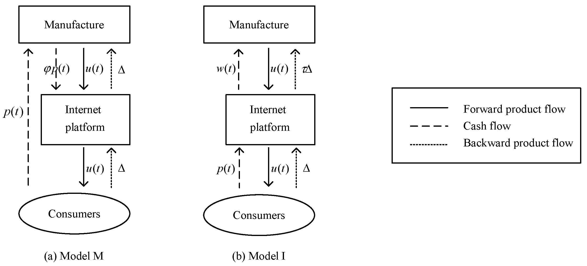
Figure 1. Two trade-in models.
Systems 13 01043 g001
Figure 2. Evolutionary trajectory of product prices.
Systems 13 01043 g002
Figure 3. Impact of quality sensitivity and market share of different types of consumers on profitability. (a) The impact of pragmatic consumers on the profitability of manufacturers in both models. (b) The impact of pragmatic consumers on the profitability of retail platforms in both models. (c) The impact of innovative consumers on the profitability of manufacturers in both models. (d) The impact of innovative consumers on the profitability of retail platforms in both models.
Systems 13 01043 g003
Figure 4. Trade-in model selection. (a) Trade-in model selection for the manufacturer. (b) Trade-in model selection for the retail platform. (c) Trade-in model selection considering economic benefits.
Systems 13 01043 g004
Figure 5. Trade-in model selection considering government subsidies. (a) η 1 < η 2 (Manufacturer’s subsidy efforts > Retail platform’s subsidy efforts). (b) η 1 = η 2 (Manufacturer’s subsidy efforts = Retail platform’s subsidy efforts). (c) η 1 > η 2 (Manufacturer’s subsidy efforts < Retail platform’s subsidy efforts).
Systems 13 01043 g005
Figure 6. Trade-in model selection considering net residual value of asymmetrically recovered products.
Systems 13 01043 g006
Table 1. Examples of trade-in service offered by real-life businesses.
ScenariosCompaniesDescriptions
Model MHP (USA-CA)HP regularly offers trade-in services for computer products, allowing market-valued second-hand devices to be exchanged for discounts on new purchases.
AT&T (USA-TX)Consumers participating in AT&T’s trade-in program can exchange their old devices for promotional cards, which can be used to pay AT&T bills, purchase new devices, or accessories.
Canon (Japan)Canon allows consumers to replace their current camera with a new or refurbished Canon camera at a discounted price.
IBM (USA-NY)Customers in Canada and the U.S. can receive trade-in rebates from IBM if they purchase new equipment from an IBM business partner to replace older IBM equipment or competitively branded equipment.
Model IeBay (USA-CA)A program called “Instant Sale” targeting smartphones, enabling consumers participating in the trade-in to receive vouchers for purchasing new devices.
Wish (USA-CA)Starting in March 2024, customers in Europe can join in trade-in on Wish for devices such as smartphones, laptops and tablets.
Gome (HongKong)In 2016, Gome Butler, a delivery platform for high-quality home appliance after-sales service, formed a closed-loop business from the purchase of goods to re-purchase, in which “trade-in” became an important part of the service system.
Shopee (Singapore)Shopee offers trade-in programs for a variety of gaming consoles, smartphones and computer devices. Consumers who participate in the trade-in program receive “cash” directly towards the purchase of a new product.
For more details on the above trade-in examples, please visit their respective official websites.
Table 2. Symbol Definition.
SymbolDefinition
Exogenous parameter
a Market size
χ Market share of pragmatic consumers
δ Product quality decay rate
β Consumer price sensitivity
γ Innovative consumers quality sensitivities
λ Pragmatic consumers quality sensitivities
φ Commission rates for retail platform when manufacturer dominate trade-in
τ Percentage of net salvage value share of recycled products received by manufacturer when retail platform dominates trade-in
Δ Net residual value of recycled second-hand products
k Quality improvement input cost factor
q 0 Initial product perceived quality
Decision variables
u ( t ) Product quality improvement inputs, as determined by the manufacturer
p ( t ) Product sales price, as determined by the trade-in lead party
w ( t ) Wholesale price, manufacturer’s decision when retail platform dominates trade-in
State variable
q ( t ) Perceived product quality at every moment
Disclaimer/Publisher’s Note: The statements, opinions and data contained in all publications are solely those of the individual author(s) and contributor(s) and not of MDPI and/or the editor(s). MDPI and/or the editor(s) disclaim responsibility for any injury to people or property resulting from any ideas, methods, instructions or products referred to in the content.