Article

Taxi Travel Distance Clustering Method Based on Exponential Fitting and k-Means Using Data from the US and China

School of Architecture and Fine Art, Dalian University of Technology, Dalian 116024, China
*
Author to whom correspondence should be addressed.
Systems 2024, 12(8), 282; https://doi.org/10.3390/systems12080282
Submission received: 18 June 2024 / Revised: 18 July 2024 / Accepted: 1 August 2024 / Published: 3 August 2024
(This article belongs to the Section Systems Engineering)

Abstract

:
The taxi travel distance distribution can be used to forecast the origin and destination (OD) distribution of taxis and private cars. Most of the existing studies on taxi trip distributions have summarized a “low–high–low” trend and approached zero at both ends; however, they failed to explain the reason for this distance distribution. The key indicators and parameters identified by various researchers using big data for the same city and year typically differ, especially in terms of the mode and mean values of distance and time. This study uses New York yellow and green taxi data (a total of 417,018,811 data points) from 2017 to 2022, as well as data from China, to obtain a general law of the taxi travel distance distribution through an analysis of the relative distance and relative frequency. The travel mode was 0.54 times the relative distance, while the data tended towards zero at 2.0 times the relative distance. We verified the reliability of the research method based on reference and survey data. The results reveal the formation mechanism of the taxi travel distance distribution characteristics, which follow an exponential distribution. These laws can be used in the context of urban planning and transportation research. We propose a taxi form distance clustering method based on the k-means approach, chosen for its effectiveness on large datasets, interpretability, and alignment with our research objectives. This method provides visual results for the travel distance and accurate information for urban transportation planning and taxi services. The practical implications for policymakers, urban planners, and taxi services are discussed, demonstrating how the identified travel distance distribution laws can influence urban planning and taxi service optimization. Finally, the problems of data collection, cleaning, and processing are identified from the perspective of data statistics and analysis.

1. Introduction

Taxis are a type of urban public transportation with the individual mobility attributes of motorized travel. The travel trajectory and time of taxis equipped with GPS and online car-hailing (OCH) platforms can be accurately obtained directly through the use of mobile applications. These positioning and travel data are accurate and easy to obtain, and taxi data are an essential resource for studying the travel characteristics and laws of taxis and individual motorized transportation [1,2,3]. Moreover, the trip distribution characteristics of taxis are similar to those of other motor vehicles and can reflect the urban traffic conditions, urban spatial structure, and resident travel information. Understanding the laws of travel patterns could have impacts on epidemic prevention, emergency responses, urban planning, and agent-based modeling of human mobility. Numerous papers have been published on taxis in relation to urban mobility, and this continues to be a significant area of interest [4].
Urban transport travel research has evolved from traditional traffic surveys to the use of big-data-based statistics. Innovations in information and communication technologies have presented opportunities to improve traffic systems and significantly impact the taxi industry. Mobile phone trace data can reasonably represent individual mobility and complement conventional travel surveys in mobility studies [5]. Differences in data collection methods between traditional resident travel surveys and big data lead to different statistical results for travel time and distance. Multiple studies have shown that the taxi travel distance follows an exponential distribution, while travel time follows a power distribution. Due to differences in classification intervals, the fitting results and effects for the same city can vary [2,6,7].
To date, research on taxis has mainly concentrated on the fields of statistics, behavior, urban transportation, and planning [8,9]. Travel behavior can be analyzed through travel distance, time, and speed distribution characteristics [10,11]. We used data from New York City, USA, as well as various cities in China to conduct our analysis. The travel distance of taxis affects the choice of travel method and its frequency of use; for example, people are inclined to choose taxis for long-distance business trips [12]. The taxi travel distance also affects the pickup rate, which determines the driver’s income [13]. These are common concerns for taxi drivers and passengers.
Taxis tend to cover a wide geographic area. Qian and Kikusui [14] indicated that taxi travel is related to urban morphology, but no specific formula was presented. Zhan [15] studied the travel time of New York City (NYC) taxis and constructed a link travel time estimation model to predict taxi travel times; however, travel time is more complex than travel distance. Even under clear path conditions, delays caused by real-time road conditions can cause the predicted values to be inconsistent with actual values, resulting in difficulties in understanding the principles affecting travel time. Kamga [13] used NYC data from 2010 to study the impact of weather on taxis. Unlike annual weather impacts, taxi travel laws are related to the size and development of a city; thus, data must be collected continuously in the same city for many years.
The random forest (RF) model has been utilized to investigate the selection of short-distance travel modes in specific cities [16]. Studies have delved into the impact of travel time and costs on commuting decisions [17]. Clustering methods have recently been widely applied to explore hidden information in large-scale trajectory data, thereby uncovering travel patterns [18]. For example, trajectory clustering methods [19] and mean clustering algorithms [20] have been used to identify clusters of homogeneous vehicle trajectories. However, these methods have limitations in determining short-distance patterns and struggle to pinpoint accurate cluster centers.
To address the aforementioned issues, we took NYC, USA as an example and collected 6 years of taxi data from 2017 to 2022, along with data from various cities in China. We collected data from different years, countries, cities, and stages, and the taxi travel distance distribution patterns based on these data were found to have common characteristics. We also propose a relative distance method, which can effectively simulate and analyze multi-year, country, city, and stage data (including NYC taxi travel data), in order to obtain the general law of the taxi travel distance distribution. At the beginning of a statistical analysis, researchers should define a unified scale to ensure that the research process and conclusions will be substantially close to the objective facts. We propose a taxi driving distance clustering method based on k-means clustering, which was chosen due to its effectiveness on large datasets, interpretability, and alignment with our research objectives. Visualizing the clustering results enables one to easily understanding the patterns present in the data, revealing associations between different clusters.
The main contributions of this paper can be summarized as follows:
  • We introduce a relative distance method to analyze and model the taxi travel distance distribution, providing a unified approach for handling multi-year and multi-city data.
  • We propose a taxi travel distance clustering method based on the k-means approach, which offers a visual and accurate classification of travel distances, aiding in urban transportation planning and service optimization.
  • We carried out extensive experiments on real taxi driving data in New York and China, in order to verify the effectiveness of our proposed method.
The remainder of this paper is structured as follows. In Section 2, we summarize the key indicators of taxi and OCH travel distances and times in different countries and cities over a period of years, and obtain a unified trip distribution. In Section 3, we process the NYC taxi travel data, perform exponential fitting to obtain the relationship between travel distance and travel frequency, and outline the relative distance method. In this section, we also propose a taxi form distance clustering method based on k-means clustering for automatic classification of the driving distance. In Section 4, we detail the reasonable parameter range obtained through trial calculations, the general law of taxi travel distance, and the fitting and clustering results. Finally, in Section 5, we present the conclusions.

2. Background

The statistical results presented in existing studies vary due to different processes and methods of data collection and processing. Some modes are formatted as fixed values, while others are initial and terminal values. Given the differences in the classification interval, the fitting results and effects within the same city may differ [2,6,7]. The mode and average determined in the same city and in the same year by different authors are often different, as shown in Table 1; for example, the average taxi travel distances in Beijing were determined as 6.53 km [7] and 8.60 km [21] in 2015; the mode values in Shanghai were 3.00–6.00 km [22] and 1.85 km [23] in 2015; and the mode values were 4.50 km [24] and 4.00 km [25] in 2016 in Chengdu.
Both the average and mode distances can represent the central tendency of the data, but a significant gap may be observed in the same year; for example, the average for Beijing in 2015 was 6.53 km, while the mode was only 1.90 km [7], indicating a high proportion of long-distance travel. However, this result was not consistent with the reality in Beijing. Similarly, the average values for Shanghai in 2014 and Xi’an in 2013 were 7.00 km [26] and 5.08 km [27], respectively, while their modes were in the range of 3–4 km, which may reflect the statistical method used. There has been slightly less research on taxi travel time than travel distance, as the same travel path can yield significant differences in travel time due to different travel conditions (e.g., congestion, morning and evening peaks, flow, weather), and it is not possible to represent the laws and characteristics of travel solely based on travel time data. In the existing studies, the average and mode obtained for OCH have been slightly lower than those of taxis, due to their respective billing methods [28].
Taxi data collection is mainly based on the location of the origin and destination, while OCH tends to use the full trip order itinerary to calculate the travel distance. In areas with poor GPS signal (e.g., underpasses, bridges, suburbs), data interruptions may occur. For example, the mode distance of Beijing OCH (2016) was substantially higher than that for taxis (2015) [7,21]. Newly developed OCH platforms can directly obtain the travel distance and time data from a platform through the use of mobile phone applications. This process involves combining the origin and destination of the trip with a map of the city, which is more accurate than the data determined by taxis through GPS, location information, and speed changes.
After analyzing the preceding research data, the travel distance distributions of taxis and OCH can be explained. Although the values were different, the distribution patterns all showed a “low–high–low “ trend, with the two ends tending to be close to zero. The similarity of these distributions indicated that taxi travel distances share commonalities.
Figure 1 summarizes the travel distance distribution for taxis and OCH in different countries and cities over a period of years. Although the modes for China and the U.S. were different, due to differing billing methods and travel behavior characteristics in the different countries, the overall distributions were similar.
Table 1. Critical indicators of travel distance and time of taxis and OCH in different countries and cities for years.
CityYearAverage
Distance
Mode
Distance
IntervalOrder Type
Beijing [7]20156.53 km1.90 km2.00 km/10.00 kmTaxi
Beijing [21]20158.60 km--Taxi
Beijing [21]201617.70 km10.00 km2.00 kmOCH
Beijing [28]2015---Taxi
Beijing [28]2016---OCH
Shanghai [26]20147.00 km3.00–4.00 km1.00 km/3.00 kmTaxi
Shanghai [23]20158.69 km3.00–6.00 km3.00/4.00/5.00 kmTaxi
Shanghai [24]2015-1.85 km5.00 kmTaxi
Xian [27]20085.75 km--Taxi
Xian [29]2011-0–2.00 km2.00 kmTaxi
Xian [30]2011-0–2.00 km2.00 kmTaxi
Xian [27]20135.08 km3.00–4.00 km1.00 kmTaxi
Chengdu [24]2016-4.50 km3.00 kmTaxi
Chengdu [25]20165.00 km4.00 km10.00 kmOCH
Harbin [10]2012-3 km-Taxi
Qingdao [31]20157.20 km--Taxi
Nanchang [32]20196.80 km3.00–6.00 km3.00 kmTaxi
San Francisco [6]2008-1.30 km5.00 kmTaxi
San Francisco [33]20146.20 km
5.10 km
-
-
-
-
Taxi
Taxi (ridesourcing)
New York [26]20144.83 km0–3.00 km-Taxi
Chicago [34]2019
2019
6.94 km
7.98 km
1.00–2.00 km
1.00–2.00 km
1.00 km
1.00 km
Taxi
OCH
Travel cost also affects people’s choices and behaviors. For example, the share rate of taxis in Beijing decreases with an increase in the taxi starting price and unit price per kilometer. The higher the taxi cost, the more people tend to choose OCH. However, due to the increased travel time and vehicle demand during peak hours, people will also choose taxis for reasons of convenience. The travel mode is closely related to the distance specified by the minimum taxi fee.
However, there are also issues in various studies that cannot be reasonably explained; for example, a periodic downward trend is typically observed before the mode. At the city boundary (about 20 km), some scattered points do not follow the distribution law. Moreover, the value on the y-axis is not zero when x = 0. On the basis of these problems, we selected the travel distance data of taxis in NYC in 2017–2022 for further verification.

3. Methodology

3.1. Mode-Aware Travel Distance Fitting

In light of the observed variations in the taxi travel distance distribution, due to the existence of abundant travel data with varying degrees of accuracy—especially in such a dynamic city such as NYC, where the classification intervals play a crucial role—it is evident that the mode of travel distance is influenced by these factors. The discrepancies in findings across different studies investigating taxi travel data within the same city and year can be partially attributed to these variations. Consequently, the current research aimed to address this variability through introducing a mode-aware travel distance fitting method, taking into consideration the nuanced characteristics of taxi travel patterns in NYC.
We first define the travel distance modes to model the distribution of travel distances. Let D(x,y) symbolize the travel distance distribution, with x and y signifying the lower and upper bounds of the distance interval, respectively. The travel distance mode d is defined as d = y − x (we provide detailed settings for six travel distance modes in the experiment section).
Liang [2] and Wang [6] stated that taxi travel distance follows an exponential distribution. Veloso [3] showed that the decreasing interval of taxi trip distances could be fitted with an exponential distribution. Liang [2] demonstrated that a power law distribution performed worse. Wang [6] reached a similar conclusion: displacement distributions of human travel by taxi tend to follow exponential laws rather than power laws. Overall, the effect of exponential fitting can be better, when compared with that of traditional methods. Hence, the NYC taxi travel distance data were fitted with an exponential distribution in this study. The formulas of the EXP fitting of yellow taxis (1) and green taxis (2) can be expressed as follows:
fd(x1)yellow = a1EXP(b1 × 1),
fd(x2)green = a2EXP(b2x2),
0.5 km ≤ x1, x2 ≤ 70 km,
where x is a variable and a and b are parameters of an exponential distribution. Exponential fitting usually involves using such methods as maximum likelihood estimation (MLE) to find the most suitable parameter values, making the model more likely to produce observed data. Performing exponential fitting on taxi travel distance means fitting the taxi travel distance data into an exponential distribution, to better understand and describe the distribution characteristics of these distances. This fitting method can be used to capture the probability distribution of taxi travel distance, providing a basis for further analysis and modeling.

3.2. Modified Exponential Fitting Optimization

Gonzalez [4] indicated that after correcting for differences in travel distances, human trajectories show a high degree of spatial regularity; that is, the mobility of humans follows simple, reproducible patterns. Jiang [35] illustrated that taxi travel presents a scaling property, which can be attributed to the spatial distribution in selection intervals. We used the aforementioned similarity and regularity as a basis to further explore analytical methods at the urban scale. The distribution of human intra-urban travel follows an exponential law related to city size [36].
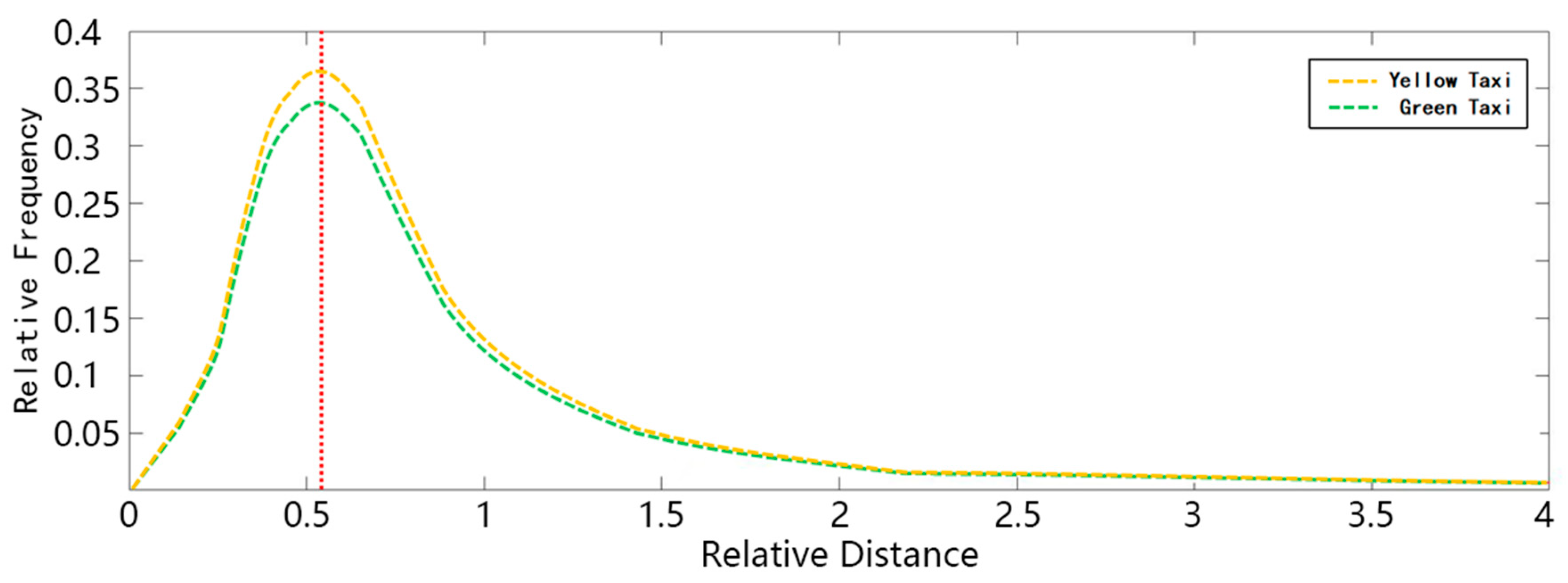
We quantitatively analyzed the aforementioned law and obtained the corresponding formula. First, the travel distance distribution of taxis in NYC from 2017 to 2022 had common features with previous studies: a “low–high–low” trend and both ends approaching zero. Data for years, countries, cities, and stages had stable and similar distributions. These data were fitted exponentially, and the obtained results were good. After continuously changing and adjusting the formula, we proposed the concept of relative distance, and processed the research data at a unified scale. The relative distance, Lr, is obtained as the ratio of the distance of a specific travel mode to the average distance of this travel mode. The relative percentage of the unit statistical interval was the relative frequency Y. The fitting results are shown in Figure 2, which allowed some laws to be determined. When the mode was located at 0.55 times and 2.0 times the relative distance, the curve gradually approached 0 (this downward trend was related to the boundary of the central urban area), considering in different years and taxi operation scopes.
The relative distance distribution is shown in Figure 2. The relative distance is Lr:
Lr = x/Lm,
where x represents the distance and Lm is a characteristic distance. The model aims to determine the relative distance distribution, which is expressed as follows:
Y = aLrEXP(b × Lr),
where Y is the relative frequency, Lr is the relative distance, a is the constant, and b is the exponential parameter. The improved fitting method provides a robust foundation for quantitatively analyzing spatial regularities and also contributes to a profound understanding of the intricate dynamics underlying the travel distance distribution of taxis at an urban scale.

3.3. Travel Distance Clustering Method Based on k-Means

The first reason we chose k-means clustering method is its superiority in handling large-scale datasets, as our study covered more than 417 million taxi trip records from New York and China, and k-means can process large-scale data with an efficient computational performance, ensuring accurate analysis and understanding of the distribution pattern of taxi travel distance. Secondly, the k-means clustering method is simple to interpret, allowing for clear visualization of the clustering results. This was significant for revealing the taxi travel distance pattern, facilitating its practical application in urban planning and taxi service optimization.
Other clustering methods, such as hierarchical clustering, DBSCAN, and the Gaussian mixture model (GMM), have their unique advantages under certain conditions, but they were not suitable for our research objectives and dataset characteristics. Although hierarchical clustering is suitable for small datasets, it has a high computational cost when processing large-scale data. Although DBSCAN can identify clusters of various shapes and sizes, the complexity of parameter adjustment may limit its application to large datasets. The GMM assumes that the data come from a mixture of multiple Gaussian distributions, which may not accurately reflect the true characteristics of our taxi trip data. Therefore, the choice of k-means was not only due to its advantage in processing big data, but also as it could provide clear and interpretable clustering results, allowing us to understand and utilize the key features of the considered taxi driving data.
To fill in the gaps of k-means when applied to taxi driving distance clustering, we gained an in-depth understanding of the characteristics of the taxi trip data through the use of the k-means clustering method, an effective method for grouping similar trip data points together to reveal the underlying data patterns.
The objective function of K-means aims to minimize the sum of squares within a cluster to ensure that the driving distances within the same cluster are relatively close. The objective function can be expressed specifically as follows:
J = i = 1 N   j = 1 K w i j D i μ j 2 2 ,
where J is the objective function, N is the number of trip data points, K is the number of clusters, w i j is a binary indicator showing whether trip data point D i belongs to cluster j , μ j is the center of cluster j , and D i μ j 2 2 denotes the squared Euclidean distance.
In the context of taxi travel distance, the updating of K-means cluster centers involves computing the mean of travel distances within each cluster. Specifically, the update expression is
μ j = 1 S j i S j D i ,
where S j represents the indices of trip data points within cluster j , S j is the number of data points within the cluster, and D i is the distance of the i -th trip data point. In the context of taxi travel distance, the goal of K-means cluster assignment is to assign each trip data point to the cluster whose center is closest. Specifically, the expression for cluster assignment is
w i j = { 1 ,      if   j = argmin k D i μ k 2 2 0 ,                 otherwise   ,  
where argmin denotes the index of the cluster with the minimum distance. Through these K-means clustering methods, we gain deeper insights into the internal structure of taxi trip data and the distribution characteristics of travel distances, providing more specific information and insights for urban transportation planning and taxi services.

4. Experiments and Results

Taxi datasets have problems related to the two stages of data collection and processing, which affect the overall data quality. Moreover, there may be conceptual misunderstandings. Similar to taxis, different transportation modes and urban data dominated by GPS also encounter these problems.

4.1. Data Collection

The collection mechanism of GPS data for taxi companies involves tracking the location every 5 s while the vehicle is in motion and every 10 s when the car is stationary (https://gpsgate.com/, accessed on 30 August 2023.) [37]. Taxi GPS data may have insufficient continuity, due to signal loss caused by high buildings, terrain, malfunctioning of GPS devices, or human error (e.g., taxi drivers forgetting to log the end of a trip) [38]. In addition, one trip may be counted as two trips due to missing values, leading to the average distance being smaller than it is in reality. Household survey data, which could be used for validation, typically fail to include short-distance travel. Although providing the travel distance, big data generally lack information on travel confirmation, travel purpose, and related variables. The drawbacks of resident trip surveys include distance inaccuracies and insufficient data. These issues may necessitate analytical processing before meaningful information can be derived from the data. In addition, the data include the cost of taxis over the distance traveled, which can be used to identify changing patterns in cost over different distances traveled.

4.2. Data Processing

Intervals affect the data processing results. According to the 2017 National Household Travel Survey (NHTS;US Department of Transportation 2017), the mode of the vehicle trip distance in NYC was 1.6 km, while the values of different classification intervals were 0.95, 1.05, 1.25, 1.50, 4.50, and 2.50. Only the value of 1 km was close to the American mode. The NHTS survey is conducted door-to-door or via email every 5–8 years to obtain travel data and tends to closely reflect reality. Through the preceding comparison, we found that the selection of data processing intervals affected the obtained conclusions. Some studies also indicated that the interoperability of data processing is related to the various formats of the original data [32]. Therefore, it is imperative to process data at a unified scale.
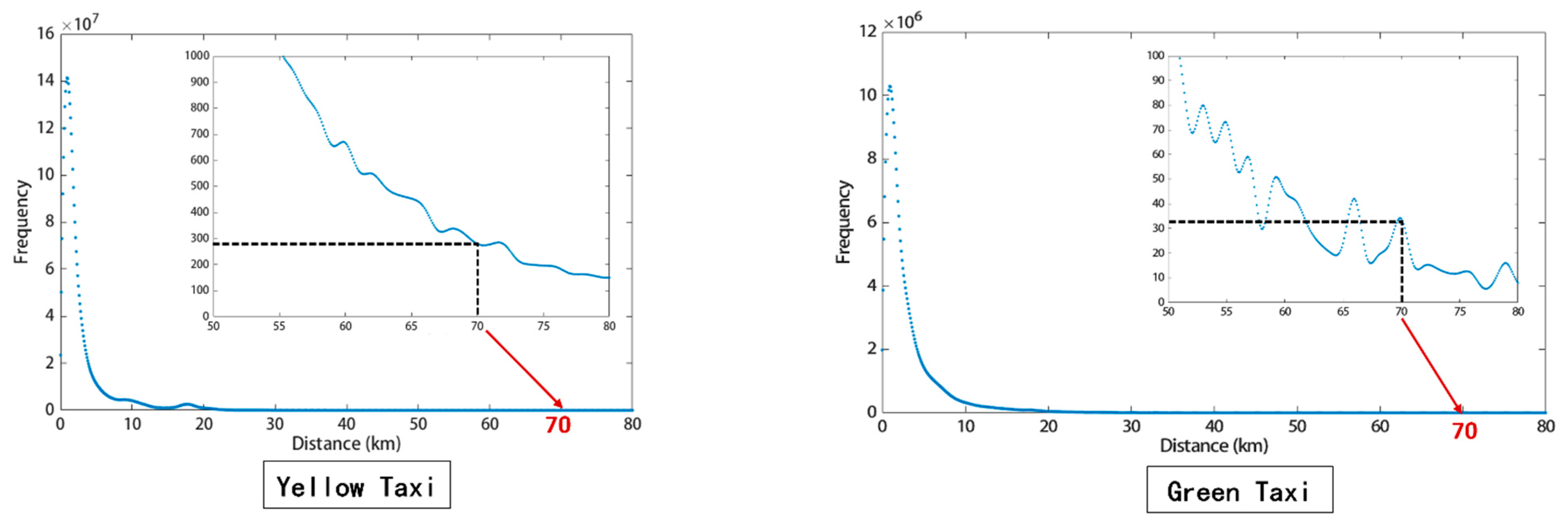
NYC is known for its visible taxi traffic, and yellow taxis have become symbolic of the city [13]. The data used in this study reflect the NYC taxi order (for a total of 13,587 data points) from 2017 to 2022, including yellow and green taxis. Yellow taxis can run throughout the city, while the operation area of the green taxis includes northern Manhattan (above E 96th St and W 110th St) and the outer boroughs. The data used in this research were collected from the NYC Taxi and Limousine Commission (TLC) website: https://www.nyc.gov/site/tlc/about/tlc-trip-record-data.page (Accessed on 24 April 2023). Technology providers were authorized under the Taxicab and Livery Passenger Enhancement Programs (TPEP/LPEP). Through preliminary sorting of the data, we found that, when the distance (x-axis) was 0, the frequency (y-axis) was not 0; that is, some orders did not generate a travel distance, which cannot be reasonably explained and should be classified as invalid orders. In addition, an extreme value (≥600 km) existed, which may have represented inter-city travel. We selected data between 0.5 and 70 km for the analysis. The selection of the minimum was based on the distance to the public transportation station, and the maximum was based on the size and boundaries of the city. Figure 2 shows the selection criteria for the boundary values.
We filtered and cleaned the two sets of data, and the results are shown in Table 2. We obtained a total of 378,573,556 data points from yellow taxis (95.62% average effective rate; AER) and 27,814,750 from green taxis (93.08% AER).

4.3. Analysis of Travel Distance Modes

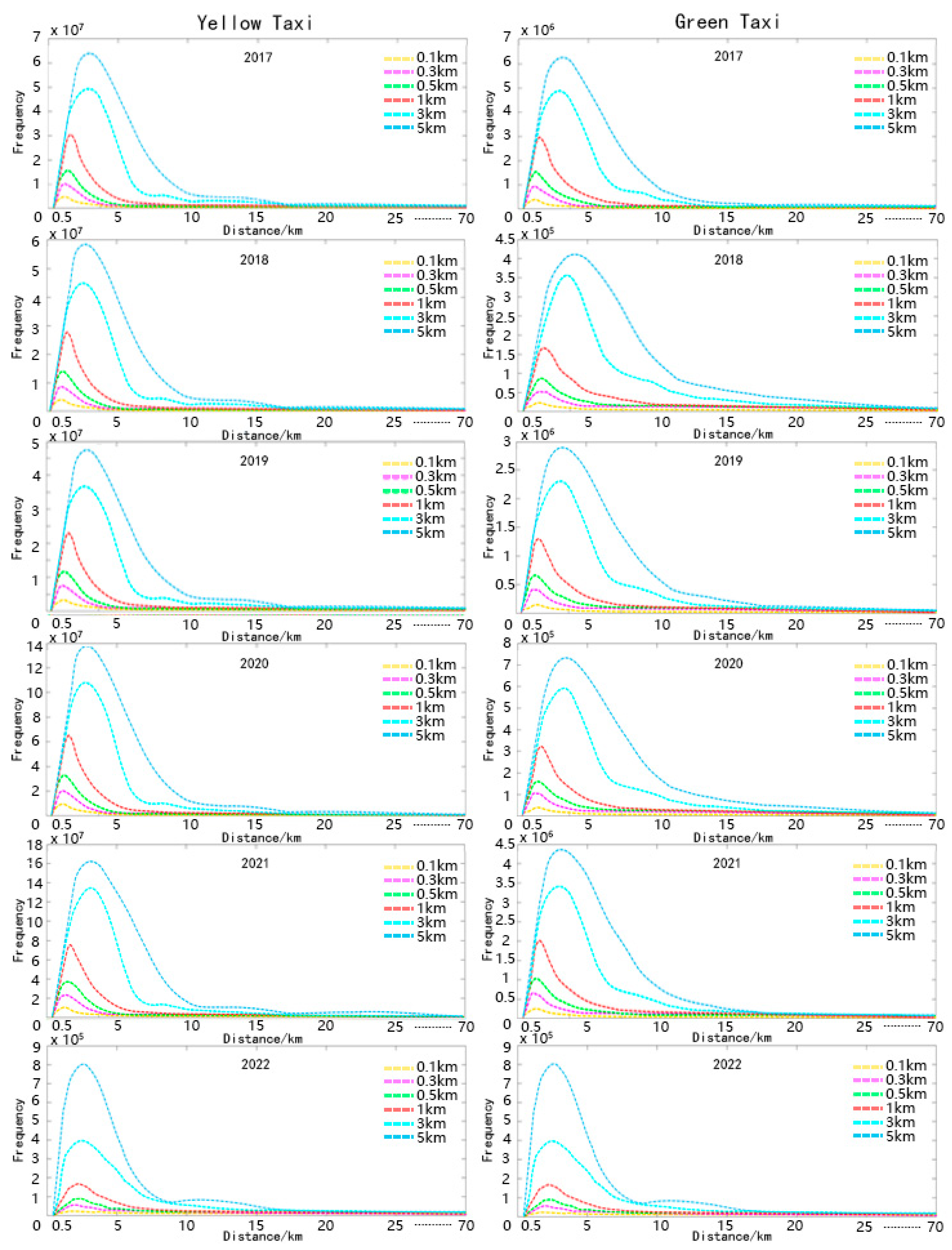
As shown in Figure 3, we set the travel distance mode classification interval d to {0.1, 0.3, 0.5, 1, 3, 5} in order to calculate the distance distribution. The overall trip distribution trend of the two types of taxis over five years was similar, but the modes of the different classification intervals were different. Among the yellow taxi data, the modes of the same classification intervals were the same: 1.45 km for a 0.1 km interval, 1.55 km for a 0.3 km interval, 1.75 km for a 0.5 km interval, 2.00 km for a 1.00 km interval, 5.00 km for a 3.00 km interval, and 3.00 km for a 5.00 km interval, respectively. Data for the green taxis were still different: 2.35 km for a 0.1 km interval, 2.45 km for a 0.3 km interval, 2.25 km for a 0.5 km interval, 3.00 km for a 1.00 km interval, 5.00 km for a 3.00 km interval, and 3.00 km and 8.00 km for a 5.00 km interval. The mean distance (Lm) was not affected by the classification interval, and it is applied as a unified scale in the following section.
Table 3 shows the modes of NYC yellow and green taxis at the six classification intervals from 2017 to 2022. For green taxis, although the data were from the same year and same city, different statistical classification methods led to different conclusions. Meanwhile, the average travel distance was almost unaffected by the classification interval (Table 4).

4.4. Fitting Results

Figure 4 shows that, the maximum occurred at the 3 km and 5 km intervals: at 5 km, the frequency reached over 0.9000. The reason for this was that most data were concentrated in the two intervals, and the fitting results for the two sets were not highly referential.
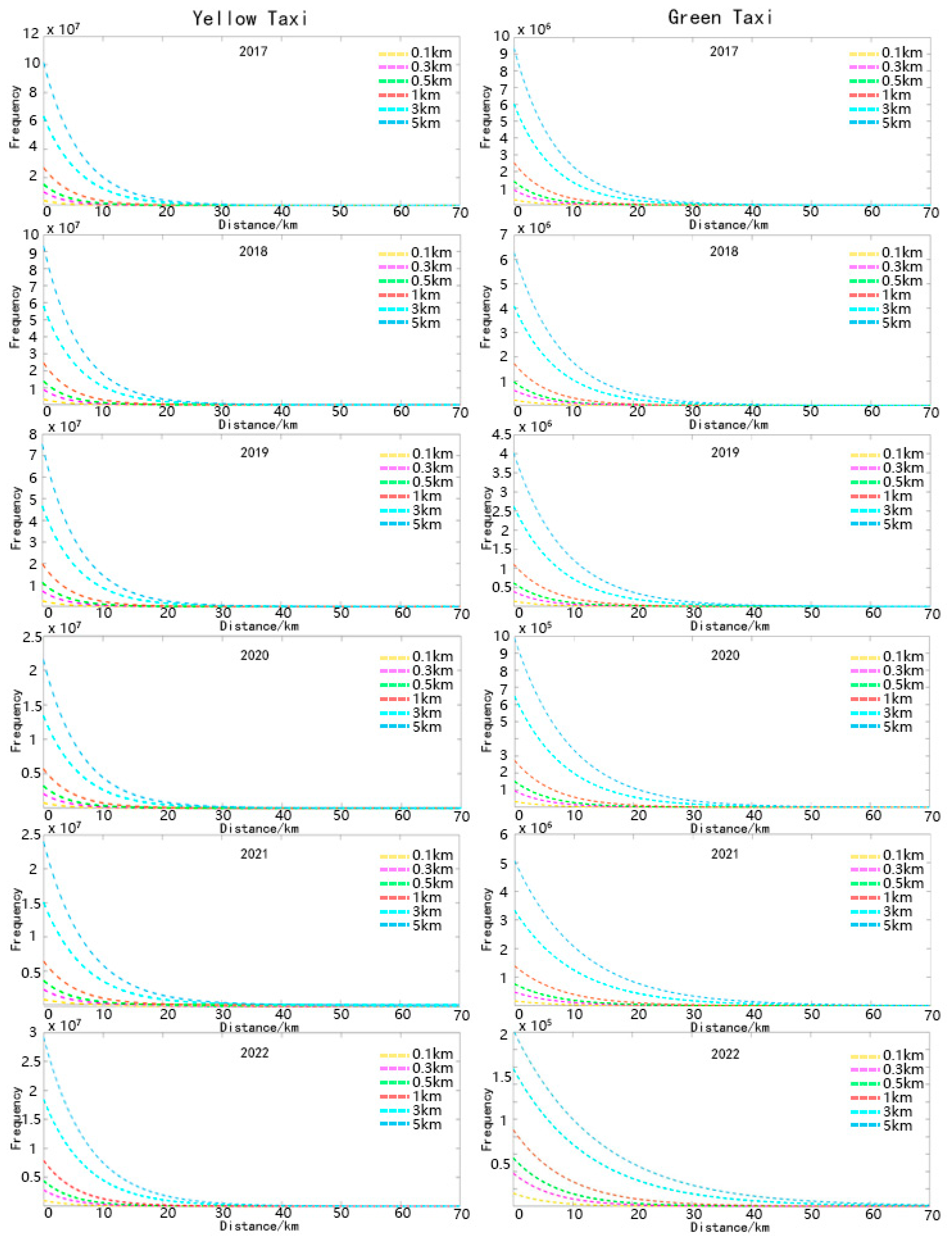
Figure 5 shows the exponential fitting results of NYC yellow and green taxis for the six classification intervals from 2017 to 2022. Note that the fitting effect was significantly influenced by the classification interval, which directly led to differences in the research results.
Table 5 shows that, at classification intervals from 0.1 km to 5 km, the exponential fitting R2 changed continually, where the lowest values for yellow and green taxis were 0.7339 and 0.7691, respectively. Therefore, this type of fitting is representative of the distribution trend of taxi travel distance, and the exponential method was selected to fit the travel distance.
In addition, the improved fitting optimization method improved the results. Through trial calculations of parameters, we found that, within the parameter range of −2.00 and −2.40, R2 tended to stabilize and obtained the best fit (Table 6). As shown in Table 6, the maximum R2 values for the yellow and green taxis were 0.8652 and 0.9033, respectively, where the corresponding parameters were −2.20 and −2.30. The corrected expression is (4), and the formulas for the relative distance of the yellow and green taxis (5) and (6) with the optimal parameters are as follows:
Yyellow = aLrEXP(−2.3 × Lr)
Ygreen = aLrEXP(−2.2 × Lr)

4.5. Travel Distance Clustering Results

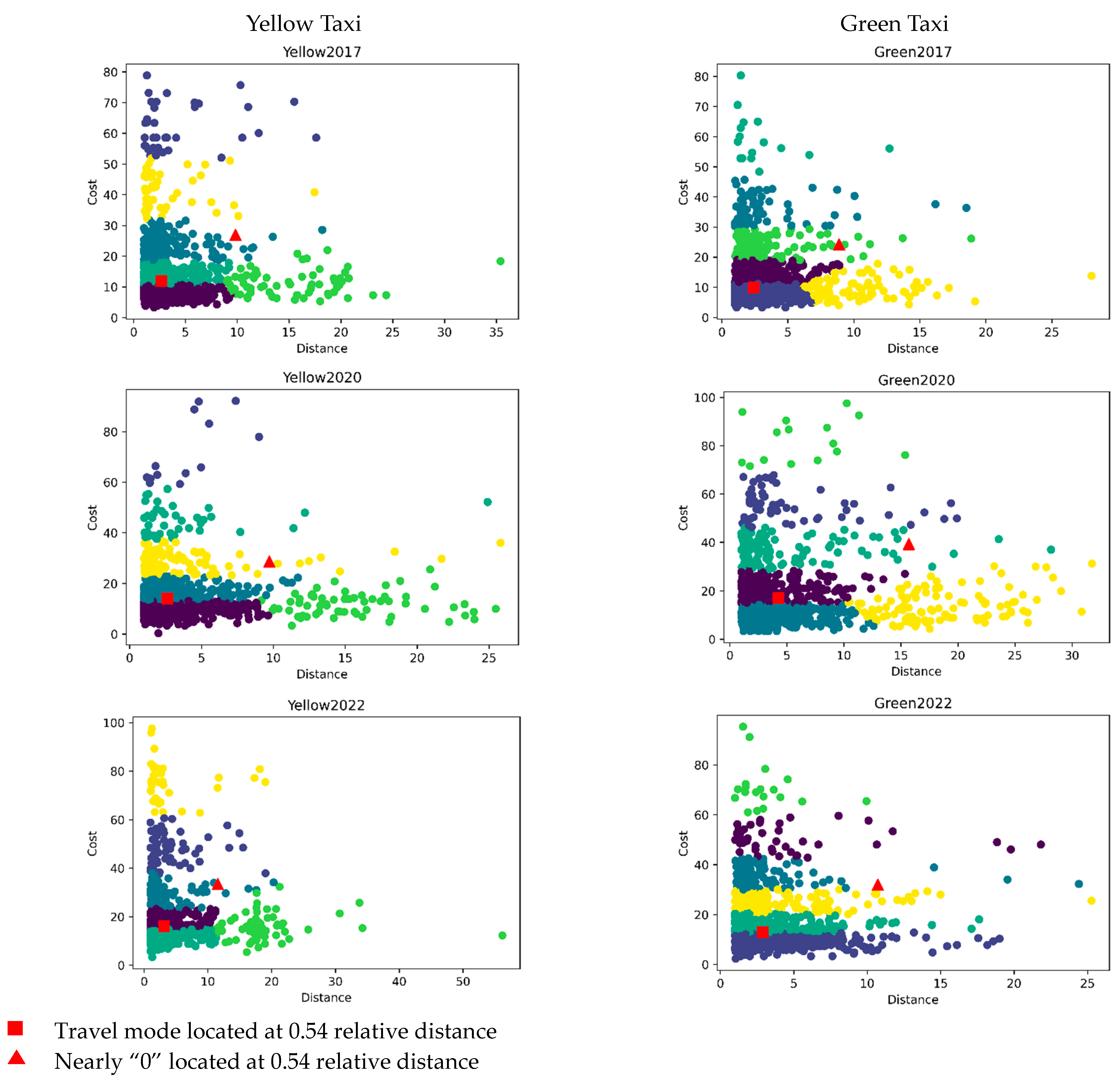
Figure 6 shows the visual experimental clustering results based on the specific data and the used clustering method. Our observations and conclusions are as follows.
Clusters with different shapes and distributions may reflect different travel distance patterns, with the highest proportion of the travel distance occurring within 10 km. High-density clusters may correspond to specific distance intervals that occur at a high frequency, providing insights into popular distances for taxi journeys. According to cost changes from 2017 to 2022, the cost of taxis was gradually increasing. In addition, distances traveled by yellow and green taxis were gradually shortening. A possible reason for this is that people prefer to take short-distance rides, while avoiding taxis when traveling long distances. Through analyzing these phenomena, we can understand the characteristics of travel distance in taxi trip data and provide additional information for urban transportation planning and taxi services. Finally, the travel mode points located at a relative distance of 0.54 (red squares in Figure 6) were the densest, while the points located at 2.0 relative distance (red triangles in Figure 6) were sparse. This result verified the effectiveness of the proposed relative distance method.

4.6. Reflections

In some practical applications, Euclidean distance is used to represent the travel distance. The Euclidean distance is the length of a straight line between the origin and destination, rather than the actual path. As such, it cannot consider detours under different traffic conditions and, so, may not adequately reflect the actual distance between different geographical locations. However, many studies have disregarded the road network between two locations in cities [37].

5. Conclusions

Transportation data can be analyzed to discover underlying trends and laws. Understanding the traffic distribution is one of the steps required for predicting traffic demand, and the average travel distance is an important indicator of the reasonable travel range for residents. These factors can be used by policymakers and urban planners. When there is a lack of data in urban or transportation planning, we can use the relative distance method to obtain the travel distribution trend based on the average taxi travel distance. In particular, the average travel distance is related to city size and, in the absence of specific average travel distances, the average distance can be inferred from the size of the central urban area, to obtain the travel distribution. Using the proposed relative distance, the average travel distance can be obtained with a smaller survey sample. Many studies have predicted the travel demand and spatial characteristics of taxis, and whether these conclusions are consistent with the overall size and local layout of the city can be verified through use of the relative distance method.
Through the analysis of taxi travel, we can learn about the behaviors of passengers, as well as people’s travel preferences and choices. Most taxi trips are occasional, and their attraction points include commercial and entertainment venues, tourist attractions, hospitals, airports, and stations. The distribution of travel distance in urban transportation planning affects the taxi volume estimate, thereby affecting the number of driver positions and the organization and planning of urban taxi transportation and facilities. Yang utilized the taxi travel distance to determine stops and design optimized routes for supermarket shuttle services [39]. Furthermore, the locations of new charging stations for electric taxis could be determined based on the average travel distance.
We observed that the distance traveled by taxis is influenced by cost (including time and fees). As costs increase, people have more options for transportation, resulting in lower acceptance of taxis. The travel distribution also reflects the acceptance of taxis among urban residents as a mode of transportation. The fares of yellow taxis in NYC have increased by 23% (https://www.nytimes.com/2022/11/17/nyregion/taxi-fare-hike-nyc.html, accessed on 17 November 2022), and the average travel distance is an important indicator of whether the base price and surcharges are reasonable.
This study collated the taxi travel data presented in previous studies and found differences in the resulting data among different research methods, management departments, cities, and years. In addition, there have been insufficient explanations for the existing research conclusions; however, the patterns of these distributions presented similarities.
We took NYC taxi distance data from 2017 to 2022 and data from various cities in China as examples for issues related to data collection, and filtered and cleaned the data. The relative distance method proposed in this study was able to partially overcome the deficiencies in data processing, and a common law of the taxi and OCH travel distance distribution pattern was obtained. In particular, the travel mode was located at 0.54 times the relative distance and, at twice the relative distance, and the data gradually trended towards zero. The utility of the relative distance method was verified using NYC and China taxi data, and the obtained data distribution conformed to the pattern proposed for the relative distance. Through trial calculations and adjustment of parameters during exponential fitting, the best parameter values of the fitting effect were byellow = −2.2 and bgreen = −2.3, and the corresponding formulas were Yyellow = aLrEXP(−2.3 × Lr) and Ygreen = aLrEXP(−2.2 × Lr). We also proposed a driving distance clustering method based on k-means clustering to visualize the automatic taxi distance clustering results. We proposed a unified rule for this travel type, which could be used to solve various urban traffic, planning, and related problems, especially in relation to taxi travel.
It should be noted that this study’s reliance on data from the U.S. and China raises the question of whether the obtained results are universally applicable. While the general principles identified may hold in other urban environments, variations in urban morphology, traffic patterns, and socio-economic factors across different countries could lead to different outcomes. Therefore, future research should extend the conducted analysis to other regions, in order to validate and potentially refine these findings.

Author Contributions

Conceptualization, Zhenang Song and Jun Cai; methodology, Jun Cai; software, Zhenang Song and Qiyao Yang; validation, Zhenang Song and Jun Cai; formal analysis, Zhenang Song and Qiyao Yang; investigation, Zhenang Song and Qiyao Yang; resources, Zhenang Song and Jun Cai; data curation, Jun Cai; writing—original draft preparation, Zhenang Song and Qiyao Yang; writing—review and editing, Jun Cai; visualization, Zhenang Song; supervision, Jun Cai; project administration, Zhenang Song; funding acquisition, Jun Cai. All authors have read and agreed to the published version of the manuscript.

Funding

Funder: National Natural Science Foundation of China. Funding number: 52278048. Host: Jun Cai. Project: Research on Planning Theory and Smart Methods for Improving Road Network Quality from the Perspective of Dual Power in Cities and Blocks.

Data Availability Statement

The data used in this paper were collected from the NYC Taxi and Limousine Commission (TLC) online. Website: https://www.nyc.gov/site/tlc/about/tlc-trip-record-data.page. Accessed on 24 April 2023. The technology providers were authorized under the Taxicab & Livery Passenger Enhancement Programs (TPEP/LPEP).

Conflicts of Interest

The authors declare no conflicts of interest.

References

  1. Liu, X.; Gong, L.; Gong, Y.; Liu, Y. Revealing travel patterns and city structure with taxi trip data. J. Transp. Geogr. 2015, 43, 78–90. [Google Scholar] [CrossRef]
  2. Liang, X.; Zheng, X.; Lv, W.; Zhu, T.; Xu, K. The scaling of human mobility by taxis is exponential. Phys. A Stat. Mech. Its Appl. 2012, 391, 2135–2144. [Google Scholar] [CrossRef]
  3. Veloso, M.; Phithakkitnukoon, S.; Bento, C.; Fonseca, N.; Olivier, P. Exploratory study of urban flow using taxi traces. In Proceedings of the First Workshop on Pervasive Urban Applications (PURBA) in conjunction with Pervasive Computing, San Francisco, CA, USA, 12–15 June 2011. [Google Scholar]
  4. Vizuete-Luciano, E.; Guillén-Pujadas, M.; Alaminos, D.; Merigó-Lindahl, J.M. Taxi and urban mobility studies: A bibliometric analysis. Transp. Policy 2023, 133, 144–155. [Google Scholar] [CrossRef]
  5. Calabrese, F.; Diao, M.; Di Lorenzo, G.; Ferreira, J., Jr.; Ratti, C. Understanding individual mobility patterns from urban sensing data: A mobile phone trace example. Transp. Res. Part C Emerg. Technol. 2013, 26, 301–313. [Google Scholar] [CrossRef]
  6. Wang, W.; Pan, L.; Yuan, N.; Zhang, S.; Liu, D. A comparative analysis of intra-city human mobility by taxi. Phys. A Stat. Mech. Its Appl. 2015, 420, 134–147. [Google Scholar] [CrossRef]
  7. Jiang, S.; Guan, W.; Zhang, W.; Chen, X.; Yang, L. Human mobility in space from three modes of public transportation. Phys. A Stat. Mech. Its Appl. 2017, 483, 227–238. [Google Scholar] [CrossRef]
  8. Zhou, Z.; Dou, W.; Jia, G.; Hu, C.; Xu, X.; Wu, X.; Pan, J. A method for real-time trajectory monitoring to improve taxi service using GPS big data. Inf. Manag. 2016, 53, 964–977. [Google Scholar] [CrossRef]
  9. Scholz, R.W.; Lu, Y. Detection of dynamic activity patterns at a collective level from large-volume trajectory data. Int. J. Geogr. Inf. Sci. 2014, 28, 946–963. [Google Scholar] [CrossRef]
  10. Tang, J.; Liu, F.; Wang, Y.; Wang, H. Uncovering urban human mobility from large scale taxi GPS data. Phys. A Stat. Mech. Its Appl. 2015, 438, 140–153. [Google Scholar] [CrossRef]
  11. Zheng, Z.; Rasouli, S.; Timmermans, H. Two-regime Pattern in Human Mobility: Evidence from GPS Taxi Trajectory Data. Geogr. Anal. 2015, 48, 157–175. [Google Scholar] [CrossRef]
  12. Alemi, F.; Circella, G.; Handy, S.; Mokhtarian, P. What influences travelers to use Uber? Exploring the factors affecting the adoption of on-demand ride services in California. Travel Behav. Soc. 2018, 13, 88–104. [Google Scholar] [CrossRef]
  13. Kamga, C.; Yazici, M.A.; Singhal, A. Analysis of taxi demand and supply in New York City: Implications of recent taxi regulations. Transp. Plan. Technol. 2015, 38, 601–625. [Google Scholar] [CrossRef]
  14. Qian, X.; Ukkusuri, S.V. Spatial variation of the urban taxi ridership using GPS data. Appl. Geogr. 2015, 59, 31–42. [Google Scholar] [CrossRef]
  15. Zhan, X.; Hasan, S.; Ukkusuri, S.V.; Kamga, C. Urban link travel time estimation using large-scale taxi data with partial information. Transp. Res. Part C Emerg. Technol. 2013, 33, 37–49. [Google Scholar] [CrossRef]
  16. He, M.; Pu, L.; Liu, Y.; Shi, Z.; He, C.; Lei, J. Research on Nonlinear Associations and Interactions for Short-Distance Travel Mode Choice of Car Users. J. Adv. Transp. 2022, 2022. [Google Scholar] [CrossRef]
  17. Liu, S.; Zhu, J.; Easa, S.M.; Guo, L.; Wang, S.; Wang, H.; Xu, Y. Travel Choice Behavior Model Based on Mental Accounting of Travel Time and Cost. J. Adv. Transp. 2021, 2021. [Google Scholar] [CrossRef]
  18. Tang, J.; Bi, W.; Liu, F.; Zhang, W. Exploring urban travel patterns using density-based clustering with multi-attributes from large-scaled vehicle trajectories. Phys. A Stat. Mech. Its Appl. 2020, 561, 125301. [Google Scholar] [CrossRef]
  19. Liu, F.; Bi, W.; Hao, W.; Gao, F.; Tang, J. An Improved Fuzzy Trajectory Clustering Method for Exploring Urban Travel Patterns. J. Adv. Transp. 2021, 2021. [Google Scholar] [CrossRef]
  20. Chen, H.; Yang, C.; Xu, X. Clustering Vehicle Temporal and Spatial Travel Behavior Using License Plate Recognition Data. J. Adv. Transp. 2017, 2017. [Google Scholar] [CrossRef]
  21. Yu, B.; Ma, Y.; Xue, M.; Tang, B.; Wang, B.; Yan, J.; Wei, Y.-M. Environmental benefits from ridesharing: A case of Beijing. Appl. Energy 2017, 191, 141–152. [Google Scholar] [CrossRef]
  22. Lv, Z.; Wu, J.; Yao, S.; Zhu, L. FCD-based analysis of taxi operation characteristic: A case of Shanghai. J. East China Norm. Univ. (Nat. Sci.) 2017, 5, 133–144. [Google Scholar]
  23. Wang, W. Study on the Calculation of Urban Accessibility Based on Taxi Trajectory; Chang’an University: Xi’an, China, 2018. [Google Scholar]
  24. Liu, H.; Liu, P.; Zhang, T. Research on travel patterns of urban population based on taxi GPS data. Jiangsu Sci. Technol. Inf. 2019, 6, 48–51. [Google Scholar]
  25. Zhang, B. Analysis of Temporal and Spatial Characteristics of Residents’ Travel Based on Online Car-Hailing Data; Southeast University: Nanjing, China, 2019. [Google Scholar]
  26. Ge, W.; Shao, D.; Xue, M.; Zhu, H.; Cheng, J. Urban taxi ridership analysis in the emerging metropolis: Case study in Shanghai. Case Stud. Transp. Policy 2020, 8, 173–179. [Google Scholar] [CrossRef]
  27. Xin, F.U.; Yu, Y.A.; Hao, S.U. Structural complexity and spatial differentiation characteristics of taxi trip trajectory network. J. Traffic Transp. Eng. 2017, 4, 106–116. [Google Scholar]
  28. Cui, Y.-C.; Guan, H.-Z.; Si, Y.; Qin, Z.T. Residents’ Travel Characteristics Based on Order Data of On-Line Car-Hailing: A Case Study of Beijing. Transp. Res. 2018, 5, 20–28. [Google Scholar]
  29. Dua, Z.; Chen, Z.; Chen, Z.; Kang, J. Analysis of Taxi Passenger Travel Characteristics Based on Spark Platform. Comput. Syst. Appl. 2017, 3, 37–43. [Google Scholar]
  30. Chen, Z. Research on Extraction and Analysis of Taxi Passenger Travel Characteristics Based on Big Data; Chang’an University: Xi’an, China, 2017. [Google Scholar]
  31. Wang, Z.; Zhang, Z.; Zhuo, B. Research on urban travel characteristics based on multi-source big data—Taking Qingdao as an example. In Proceedings of the China Urban Transport Planning Annual Conference, Chengdu, China, 14 June–16 July 2019. [Google Scholar]
  32. Luo, J.; Pan, J. A Method of Taxi Characteristics Analysis Based on GPS Data Mining. Traffic Transp. 2020, 33, 49–54. [Google Scholar]
  33. Rayle, L.; Dai, D.; Chan, N.; Cervero, R.; Shaheen, S. Just a better taxi? A survey-based comparison of taxis, transit, and ridesourcing services in San Francisco. Transp. Policy 2015, 45, 168–178. [Google Scholar] [CrossRef]
  34. Wang, Z.; Zhang, Y.; Jia, B.; Gao, Z. Comparative Analysis of Usage Patterns and Underlying Determinants for Ride-hailing and Traditional Taxi Services: A Chicago Case Study. Transp. Res. Part A Policy Pract. 2024, 179, 103912. [Google Scholar] [CrossRef]
  35. Jiang, B.; Yin, J.; Zhao, S. Characterizing the human mobility pattern in a large street network. Phys. Rev. E 2009, 80, 021136. [Google Scholar] [CrossRef]
  36. Kang, C.; Ma, X.; Tong, D.; Liu, Y. Intra-urban human mobility patterns: An urban morphology perspective. Phys. A Stat. Mech. Its Appl. 2012, 391, 1702–1717. [Google Scholar] [CrossRef]
  37. Chen, M.; Wang, N.; Lin, G.; Shang, J.S. Network-Based Trajectory Search over Time Intervals. Big Data Res. 2021, 25, 100221. [Google Scholar] [CrossRef]
  38. Neilson, A.; Indratmo; Daniel, B.; Tjandra, S. Systematic Review of the Literature on Big Data in the Transportation Domain: Concepts and Applications. Big Data Res. 2019, 17, 35–44. [Google Scholar] [CrossRef]
  39. Yang, G.; Yuan, E.; Zhang, X.; Zhou, H. A route planning mechanism for supermarket shuttle service based on taxi traces. Res. Transp. Bus. Manag. 2020, 38, 100502. [Google Scholar] [CrossRef]
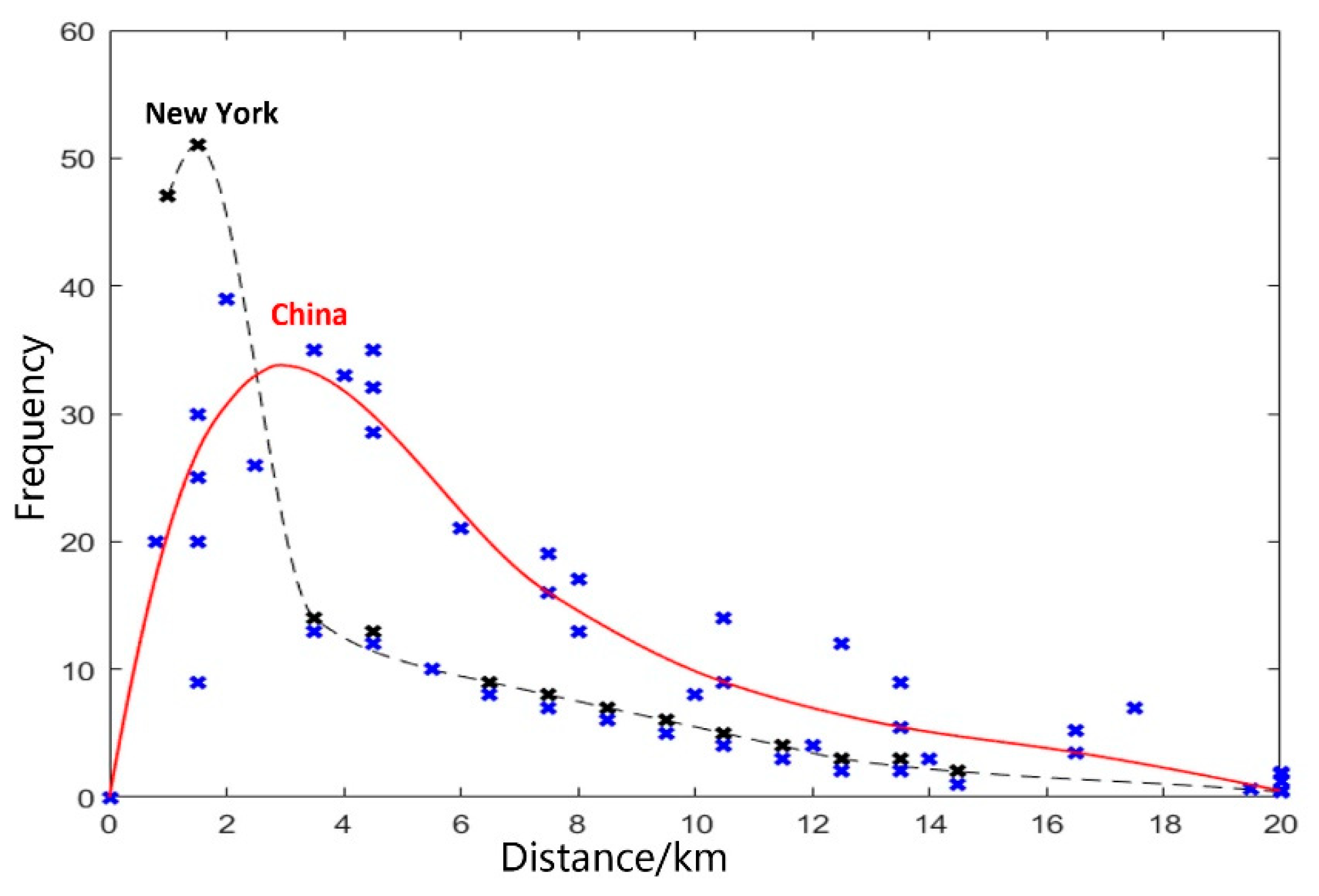
Figure 1. Travel distance distribution of taxis and OCH in different countries and cities for various years. Note: Distribution obtained from data in Table 1, represented by the symbol ×.
Systems 12 00282 g001
Figure 2. The relative distance distribution of yellow and green taxis in New York City.
Systems 12 00282 g002
Figure 3. The selection criteria for boundary value.
Systems 12 00282 g003
Figure 4. Different classification intervals of travel distance distribution in NYC.
Systems 12 00282 g004
Figure 5. Travel distance EXP fitting.
Systems 12 00282 g005
Figure 6. Cluster visualization of distance and cost.
Systems 12 00282 g006
Table 2. The result of filtering data.
YearYellow TaxiGreen Taxi
Data AmountFiltered DataEffective
Data Proportion
Data AmountFiltered DataEffective
Data Proportion
2017113,500,327107,786,05494.97%11,737,05911,079,60194.40%
2018102,871,38797,445,70494.73%8,899,7188,431,77894.74%
201984,598,44482,005,48396.93%6,300,9855,895,57393.57%
202024,649,09223,257,35594.35%1,068,755994,80693.08%
202130,904,30829,483,30195.40%705,650639,14690.58%
202239,656,09838,595,65997.33%840,402773,84692.08%
Total396,179,656378,573,55695.62%29,552,56927,814,75093.08%
Table 3. Modes of travel distance with different classification intervals in NYC.
Yellow Taxi
Mode (km) Year201720182019202020212022
Intervals
0.101.451.451.451.451.451.45
0.301.551.551.551.551.551.55
0.501.751.751.751.751.751.75
1.002.002.002.002.002.002.00
3.005.005.005.005.005.005.00
5.003.003.003.003.003.003.00
Green Taxi
Mode (km) Year201720182019202020212022
Intervals
0.101.452.351.451.452.352.35
0.301.552.451.551.552.452.45
0.501.752.251.751.752.252.25
1.002.003.002.002.003.003.00
3.005.005.005.005.005.005.00
5.003.008.003.003.008.003.00
Table 4. Average travel distance of yellow and green taxis in NYC.
Yellow Taxi
Year201720182019202020212022
Mean (km)4.914.935.084.865.335.77
Green Taxi
Year201720182019202020212022
Mean (km)4.445.376.057.845.465.36
Table 5. The EXP fitting of taxi travel distance.
YearInterval
(km)
Yellow TaxiGreen Taxi
a1b1R12a2b2R22
20170.13.506 × 106−0.27680.75463.228 × 105−0.24420.8529
0.39.722 × 106−0.25490.81259.039 × 105−0.22670.8388
0.51.507 × 107−0.23610.77491.415 × 106−0.21200.8055
12.692 × 10⁷−0.21040.75322.532 × 106−0.18850.7691
36.338 × 10⁷−0.16610.87606.030 × 106−0.15000.8837
51.017 × 10⁸−0.16210.98269.364 × 106−0.14120.9677
20180.13.227 × 106−0.28180.76782.172 × 105−0.22560.8632
0.38.938 × 106−0.25920.81456.104 × 105−0.20990.8460
0.51.384 × 107−0.23980.77629.587 × 105−0.19650.8141
12.468 × 10⁷−0.21350.75341.720 × 106−0.17480.7782
35.809 × 10⁷−0.16860.88014.081 × 106−0.13730.8824
59.341 × 10⁷−0.16490.98416.277 × 106−0.12770.9667
20190.12.596 × 106−0.27740.78661.387 × 105−0.21080.8705
0.37.202 × 106−0.25550.81343.914 × 105−0.19670.8513
0.51.117 × 107−0.23690.77546.167 × 105−0.18470.8202
11.991 × 10⁷−0.21060.74801.110 × 106−0.16450.7833
34.680 × 10⁷−0.16590.87292.630 × 106−0.12840.8709
57.539 × 10⁷−0.16260.98344.027 × 106−0.11860.9611
20200.17.415 × 105−0.26960.79973.379 × 104−0.19380.8753
0.32.064 × 106−0.24910.81689.570 × 104−0.18140.8544
0.53.211 × 106−0.23180.77921.514 × 105−0.17080.8254
15.727 × 10⁶−0.20620.74882.736 × 105−0.15240.7874
31.347 × 10⁷−0.16270.86076.484 × 105−0.11830.8576
52.162 × 10⁷−0.15880.97869.870 × 105−0.10830.9550
20210.18.138 × 107−0.23810.79271.654 × 104−0.15490.8660
0.32.288 × 106−0.22230.80484.741 × 104−0.14680.8488
0.53.591 × 106−0.20850.76937.576 × 104−0.13980.8228
16.425 × 10⁶−0.18660.73391.390 × 105−0.12660.7840
31.512 × 10⁷−0.14590.80473.332 × 105−0.09870.7917
52.401 × 10⁷−0.14110.95625.068 × 105−0.09020.9143
20220.19.929 × 105−0.23200.79271.503 × 104−0.17260.7854
0.32.795 × 106−0.21660.80003.795 × 104−0.14980.7129
0.54.389 × 106−0.20330.76535.556 × 104−0.13520.6499
17.893 × 10⁶−0.18190.72868.786 × 104−0.11320.5542
31.846 × 10⁷−0.14130.79691.581 × 105−0.07980.4445
52.918 × 10⁷−0.13600.95392.025 × 105−0.07040.4683
Note: The confidence interval is 95%.
Table 6. Comparison and selection of trial calculation parameters.
bYellow Taxi Trail R2Green Taxi Trail R2
−1.000.44840.5209
−1.100.51440.5902
−1.300.63030.7066
−1.500.72200.7933
−1.800.81440.8729
−1.900.83390.8877
−2.000.84840.8973
−2.100.85820.9024
−2.200.86360.9033
−2.300.86520.9005
−2.400.86330.8945
−2.800.82770.8451
Disclaimer/Publisher’s Note: The statements, opinions and data contained in all publications are solely those of the individual author(s) and contributor(s) and not of MDPI and/or the editor(s). MDPI and/or the editor(s) disclaim responsibility for any injury to people or property resulting from any ideas, methods, instructions or products referred to in the content.