Waiting Strategy for the Dynamic Meal Delivery Routing Problem with Time-Sensitive Customers Using a Hybrid Adaptive Genetic Algorithm and Adaptive Large Neighborhood Search Algorithm

Abstract

In this paper, we study the dynamic meal delivery routing problem (MDRP) with time-sensitive customers. The multi-objective MDRP optimization model is developed to maximize customer satisfaction and minimize delay penalty cost and riding cost. To solve the dynamic MDRP, a novel waiting strategy is proposed to divide the dynamic problem into a series of static subproblems. This waiting strategy utilizes the decision threshold to determine rerouting points based on the number of dynamic meal orders. Meanwhile, time-sensitive priority is introduced to accelerate assignment and routing decisions for orders from customers with high time sensitivity. For each static subproblem, a hybrid AGA–ALNS algorithm that incorporates the adaptive genetic algorithm and adaptive large neighborhood search is developed to improve both the global and local search capabilities of the genetic algorithm. We validate the performance of the proposed waiting strategy and the AGA–ALNS algorithm through numerical instances. In addition, managerial insights are obtained from sensitivity analysis experiments.

1. Introduction

With the continuous expansion of e-commerce, meal delivery has made people’s lives more convenient. According to a research report issued by CCFA (China Chain Store and Franchise Association) and NSRC (Ali New Service Research Centre), the Chinese online instant meal delivery market generated annual revenue of CNY 1003.6 billion (nearly USD 144 billion) in 2021, which accounted for 21.4% of the total revenue of the Chinese catering business, with a user base of 544.16 million [1]. In addition, the worldwide online meal delivery market is expected to reach USD 0.7 trillion in revenue by 2022, and the number of customers is projected to reach 2644.2 million by 2027 [2]. Numerous platforms, including Meituan and Eleme in China, as well as global meal delivery platforms like Uber Eats, Grubhub, and Door Dash, have emerged and rapidly expanded in recent years. Meituan, one of the largest meal delivery platforms in China, generated more than CNY 76.5 billion (about USD 10.6 billion) in revenue in the third quarter of 2023 [3]. Despite the considerable profits generated by the rapidly expanding instant meal delivery market, the increasing integration of meal delivery services into people’s daily lives has led customers to express higher expectations for delivery services, presenting more substantial operational challenges for platforms.

It should be noted that different customer groups are heterogeneous in their sensitivities to order delay [4,5,6]. Customers with high time sensitivity are often willing to pay additional delivery fees to enjoy their meals faster, whereas those with lower time sensitivity may accept longer delivery times for reduced delivery fees. Due to these varying time sensitivities among customers, platforms such as Uber Eats offer three options (priority, standard, and no rush) for meal delivery service to customers, as shown in Figure 1. However, a courier usually needs to perform multiple orders during the delivery process. Thus, how to generate a reasonable route to accommodate orders from customers with heterogeneous time sensitivity is a key issue that the platform needs to address.

The meal delivery routing problem (MDRP) is characterized by dynamics and stochasticity, and how to effectively deal with such characteristics of meal orders is another important issue faced by platforms [7,8]. Customers can place orders via meal-ordering applications at any time and place throughout the day. These orders typically include details such as the customer’s order time, meal type, restaurant location for pickup, and customer location for delivery. Upon receiving orders, platforms must efficiently assign them to couriers according to customer requirements. However, if couriers still have unfinished orders from previous periods, platforms need to adjust delivery routes to accommodate new orders. Notably, the number of meal orders varies at different times of the day. The study [9] points out that delivery demands present a visible tidal effect, with a sharp increase at 10:00–11:00 and 22:00–24:00 during the day. Therefore, it is another challenge for platforms to effectively handle dynamic orders during peak meal hours to avoid order delays.

With the continuous growth of the takeout market, academics are exploring possible solutions to the meal delivery problem. These studies include, but are not limited to, problems such as uncertainty in the meal delivery process [10], order assignment and route planning for couriers [11,12], and dynamic scheduling of meal orders [7]. However, these studies are based on the assumption that customers are homogeneous. Indeed, as an instant delivery service, the time-sensitive heterogeneity of customers is a crucial factor that should be considered in meal delivery. Hence, designing efficient solution strategies to serve such orders has important research implications.

To address the aforementioned issues, the meal delivery routing problem (MDRP) is investigated, which is characterized by the time-sensitive heterogeneity of customers and the dynamics of meal orders. Firstly, considering the time-sensitive heterogeneity of customers, a multi-objective optimization model is formulated to maximize customer time satisfaction while minimizing both delay penalty cost and riding cost. Secondly, a novel waiting strategy with time-sensitive priority is developed to process dynamic meal orders, which divides the dynamic problem into a series of static subproblems. In this waiting strategy, a decision threshold is introduced to determine the rerouting moment for dynamic orders. And time-sensitive priority is introduced to speed up assignment and rerouting decisions for orders belonging to customers with high time sensitivity. Finally, to solve each static subproblem, we develop a hybrid metaheuristic algorithm based on the adaptive genetic algorithm and adaptive large neighborhood search (AGA–ALNS). In AGA–ALNS, an enhanced best route with a stochastic insertion crossover (EBRSIC) operator is used to improve the algorithm’s global search capability. In addition, adaptive large neighborhood search (ALNS) is used as a mutation operator to improve the algorithm’s local search capability. Meanwhile, adaptive crossover and mutation probabilities are introduced to optimize the parameter selection of the algorithm. With dynamic MDRP instances of different scales, we illustrate the effectiveness of the waiting strategy with time-sensitive priority and the AGA–ALNS algorithm. Moreover, managerial insights are derived from sensitivity analysis experiments.

Compared with previous studies, the main contributions of this paper are summarized in three aspects. (1) We develop a multi-objective optimization model based on time-sensitive heterogeneous customers to solve the MDRP, which considers both perspectives of improving customer time satisfaction and reducing delay penalty cost and riding cost. This study enriches previous works on MDRP [7,8,13]. (2) A novel waiting strategy with time-sensitive priority is proposed, which further extends the research methods of MDRP for handling dynamic meal orders. (3) We further develop the AGA–ALNS algorithm for solving the optimization model and find the near-optimal solution for MDRP. To the best of our knowledge, this paper is one of the first attempts to solve MDRP using this hybrid approach.

The remaining structure of this paper is organized as follows. Section 2 reviews existing studies related to MDRP. Section 3 describes MDRP and defines the mathematical model of time-sensitive customer satisfaction and the operational costs of the platform. Section 4 presents the solution method of this paper, which incorporates the concepts of the waiting strategy with time-sensitive priority and the AGA–ALNS algorithm. Section 5 presents the computational experiments. Section 6 summarizes the conclusions and discusses future research directions.

2. Literature Review

In this section, we present a literature review of MDRP. MDRP is characterized by dynamically arriving orders, sharing similarities with the dynamic pickup and delivery problem (DPDP). Additionally, as an extended case of the vehicle routing pickup and delivery problem with time window (VRPPDTW), MDRP strictly regulates the order of pickup and delivery. Each order must be transported from a specific pickup location to the corresponding delivery location within a specified time interval, increasing the complexity of solving the problem. As a result, our review focuses on MDRP, DPDP, and solution methods for VRPPDTW.

2.1. Meal Delivery Routing Problem

Among the numerous relevant studies, Reyes et al. [14] first proposed the MDRP and developed a rolling-horizon repeated matching approach to solve large-scale dynamic MDRP. Yildiz and Savelsbergh [8] conducted a further investigation based on the study of Reyes et al. [14]. In contrast to Reyes et al. [14], they designed a simultaneous column- and row-generation algorithm to solve the MDRP and assumed perfect information about the order arrival. In order to avoid order delays caused by uncertain information during dynamic delivery, Ulmer et al. [7] proposed an anticipatory customer assignment (ACA) policy, which introduced a postponement to improve the flexibility of order assignment and a time buffer to reduce decisions that may cause delays. Wang and Jiang [13] developed a two-stage optimization algorithm to study customer satisfaction with time-sensitive heterogeneity. They found that considering time-sensitive heterogeneity was effective in improving customer time satisfaction. Xue et al. [10] investigated the meal delivery service with uncertain cooking time and travel time. They proposed a solution method that incorporates the island harmony search algorithm and scenario-based simulation. Bi et al. [11] established a multi-objective mathematical model to minimize customer dissatisfaction and the delivery cost for MDRP under the shared logistics services. In order to solve the proposed model, an improved ant lion optimizer (IALO) is developed. Liao et al. [15] designed a two-stage optimization algorithm for a green meal delivery routing problem to achieve objectives that maximize customer time satisfaction, courier balance utilization, and minimize carbon footprint. Wang [16] investigated three types of logistics services for multi-trip meal delivery routing problems, i.e., exclusive service and two sharing services. Through simulation analysis of real-world instances, the author found that two sharing services generated lower costs compared to the exclusive service. Tu et al. [17] studied an MDRP with dynamic arrivals for both crowdsourced couriers and meal orders. With the optimization objective of minimizing the delivery cost, a hybrid metaheuristic algorithm combining adaptive large neighborhood search (ALNS) and tabu search (TS) was proposed to solve the problem. Chen et al. [18] investigated the dynamic scheduling problem of instant delivery and proposed an online delivery scheduling algorithm with the optimization objective of minimizing the return time of the courier as well as the travel distance. Simoni and Winkenbach [12] studied the meal order assignment and route optimization problem under crowdsourcing delivery and proposed an order batching and assignment algorithm to solve the problem. Hu et al. [19] investigated the recovery management of meal delivery routes under four types of disruption events: vehicle breakdown, traffic jams, service time variation at restaurant locations, and service time variation at customer locations.

Unlike previous works such as [7,8,11,12,14], which assumed customers’ homogeneous demands, we consider the time-sensitive heterogeneity of customers when performing meal delivery routes, and develop a multi-objective optimization model for improving customer time satisfaction and reducing delay penalty cost and riding cost. Particularly, while Wang and Jiang [13] explored the MDRP considering the time-sensitive heterogeneity of customers, their study only analyzed the delivery problem for meal orders in a static scenario. In contrast, we extend their work to investigate a dynamic scenario where orders are generated dynamically.

2.2. Dynamic Pickup and Delivery Problem

In DPDPs, not all demand information can be known before the planning horizon begins, and future demand exists under a certain probability distribution. Such DPDPs are called dynamic and stochastic pickup and delivery problems [20,21]. Over the past two decades, scholars have strived to explore dynamic strategies for solving the DPDP under unknown demand information. Numerous approaches have been developed, such as the multiple scenario approach [22,23], and the waiting strategy. The waiting strategy is considered an effective method to reduce operational costs and improve service quality [24,25].

In previous studies, various waiting strategies have been explored, all focusing on deferring real-time demands and devising more efficient routes. Mitrović-Minić and Laporte [21] proposed four waiting strategies and evaluated their benefits in the dynamic pickup and delivery problem with time windows (DPDPTW). They found that the waiting strategy was effective in reducing detours and fleet size. Wong et al. [26] investigated the demand responsive transport problem in partially dynamic environments using waiting strategies. In this problem, they examined the impact on the system’s operational efficiency when the rate of dynamic demand changes. To solve the DPDP, Vonolfen and Affenzeller [25] proposed a waiting strategy that utilized historical demand information based on intensity measurement without further processing data. In a recent study, Park et al. [24] introduced a waiting strategy based on a rerouting indicator for addressing the vehicle routing problem with simultaneous pickup and delivery (VRPSPD). They argued that it is better for new demands to wait until reaching a strategically determined rerouting point, rather than be served immediately upon their arrival.

Similar to Park et al. [24], we develop a novel waiting strategy to solve the dynamic MDRP. Different from their study without time window constraints, the meal orders in this paper need to be delivered within a 40 min time window. Furthermore, our study explores the influence of customer time-sensitive heterogeneity on the waiting strategy, which is a more realistic consideration.

2.3. Solution Methods Associated with the VRPPDTW

VRPPDTW, as a variant of the vehicle routing problem (VRP) with additional constraints, is classified as an NP-hard problem. Current solution approaches for VRPPDTW primarily involve exact and metaheuristic algorithms. Exact algorithms, such as the branch-and-price algorithm [27] and the branch-and-cut algorithm [28], can achieve high-quality solutions to small-sized problems. However, as the scale of the problem increases, these exact algorithms are subjected to a sharp decrease in solution speed. Compared to exact algorithms, metaheuristic algorithms can find an approximate optimal solution within a reasonable time and are widely acknowledged as an efficient solution method.

Since the 21st century, many scholars have used some classical metaheuristic algorithms to solve the VRPPDTW, such as the particle swarm optimization (PSO) algorithm [29], variable neighborhood search (VNS) algorithm [30], and so on. In addition, some novel metaheuristics developed in recent years have also been demonstrated to be efficient methods for solving the VRP. For example, Lu et al. [31] developed a hybrid beetle swarm optimization algorithm (HBSO) to solve the 4PL routing problem. The HBSO algorithm is proposed based on the beetle antenna search (BAS) algorithm. A population search mechanism is introduced into the HBSO algorithm to improve search efficiency by turning one beetle into multiple beetles. In addition, the Dijkstra algorithm is introduced to initialize the population of the HBSO algorithm. Among numerous metaheuristic algorithms, the genetic algorithm (GA) has gained widespread application in solving the VRPPDTW due to its straightforward operation and global search capabilities. Wang and Chen [32] developed a co-evolution GA with the cheapest insertion method to solve the VRPPDTW, which generated better solutions within a reasonable time interval than the traditional GA. To solve the VRPPDTW with multi-depot, Dubey and Tanksale [33] proposed an elite GA and employed the 3-opt heuristic to further enhance the local search capability of the algorithm. One of the most important characteristics of metaheuristic algorithms is the ability to improve search performance by combining different algorithms [34]. Bi et al. [35] proposed a GA to solve an NP-hard problem with continuous domain, in which double-point crossover and non-uniform mutation operators were introduced to enhance the global and local search capabilities of the GA. To further improve the solution quality of the GA, some scholars have attempted to combine the GA with other metaheuristic algorithms. Wang et al. [36] introduced a two-stage algorithm for solving the VRPPDTW with multiple centers. In the first stage, they utilized the 3D k means algorithm to cluster the customer nodes. Subsequently, a hybrid GA–PSO algorithm is proposed to determine the routes. This hybrid approach aimed to enhance algorithm diversity and solution efficiency by employing coordinated operators between the GA and PSO. Zarouk et al. [34] developed a hybrid metaheuristic algorithm named MOGASA, which is based on the combination of GA and simulated annealing (SA). This hybrid approach harnesses the global and local search capabilities of both metaheuristic algorithms. Ren et al. [37] hybridized the fast elitist non-dominated sorting genetic algorithm (NSGA-II) with VNS for improving the search efficiency of the multi-objective GA.

Previous studies have continuously pursued the improvement of traditional GA to efficiently solve the VRPPDTW [34,36]. In this paper, we introduce a hybrid AGA–ALNS algorithm to solve the MDRP. Based on the framework of traditional GA, we enhance the algorithm’s global and local search capabilities by refining the crossover and mutation operators. In addition, adaptive crossover and mutation probabilities are introduced to avoid solution quality degradation caused by improper probability value setting. To the best of our knowledge, none of the studies have employed this hybrid AGA–ALNS algorithm to solve the MDRP.

With the above literature review, we compare this study with previous works in terms of the studied problem, objectives, problem characteristics, and solution methods. The summarized information is presented in

Table 1. Comparison of this study with related literature.

Reference	Problem	Objectives			Problem Characteristics					Solution Methods
		CS	DP	RC	THC	DD	TW	PD	MO	DDP	Algorithm
Ulmer et al. [7]	MDRP		✓			✓	✓	✓		MDP	Heuristic
Yildiz and Savels-bergh [8]	MDRP		✓				✓	✓			Exact
Bi et al. [11]	MDRP	✓		✓			✓	✓	✓		IALO
Simoni and Winken-bach [12]	MDRP			✓		✓	✓	✓	✓	RH	Heuristic
Wang and Jiang [13]	MDRP	✓			✓		✓	✓			GA
Reyes et al. [14]	MDRP		✓			✓	✓	✓		RH	Heuristic
Mitrović-Minić and Laporte [21]	DPDP			✓		✓	✓	✓		WS	TS
Park et al. [24]	DPDP			✓		✓		✓	✓	WS	GA
Vonolfen and Affen-zeller [25]	DPDP			✓		✓	✓	✓		WS	Heuristic
Dubey and Tanksale [33]	VRPPDTW		✓	✓			✓	✓			GA
Wang et al. [36]	VRPPDTW		✓	✓			✓	✓	✓		GA–PSO
Zarouk et al. [34]	VRPPDTW	✓	✓	✓			✓	✓	✓		MOGASA
This work	MDRP	✓	✓	✓	✓	✓	✓	✓	✓	WSTP	AGA–ALNS

Note: CS: Customer satisfaction; DP: Delay penalty cost; RD: Riding cost; THC: Time-sensitive heterogeneity of customers; DD: Dynamic demands; TW: Time window; PD: Pickup and delivery; MO: Multiple objectives; DDP: Dynamic demand process method; RH: Rolling horizon method; MDP: Markov decision process; WS: Waiting strategy; WSTP: Waiting strategy with time-sensitive priority.

. Our study stands out by integrating various factors such as time-sensitive heterogeneity of customers, dynamic demands, time window, pick and delivery, multiple objectives, and waiting strategy into the MDRP. None of the previous studies included all of these factors simultaneously. In summary, this study first investigates the time-sensitive heterogeneity of customers and develops a multi-objective model from the perspectives of customer time satisfaction as well as delay penalty cost and riding cost. Secondly, a novel waiting strategy is proposed to handle dynamic meal orders. The concept of time-sensitive priority is introduced to optimize order assignment and rerouting decisions for customers with time-sensitive heterogeneity. Finally, a hybrid AGA–ALNS algorithm is proposed to optimize the delivery routes for couriers.

3. Problem Statement and Modelling

In this section, we first give a detailed problem statement of the MDRP and then present the relevant settings for the dynamic problem. Afterward, the mathematical formulation of the static subproblem is presented in detail.

3.1. Problem Statement

In this paper, we study the dynamic MDRP with time-sensitive customers. We consider three types of customers with high, medium, and low time sensitivity. The higher the time sensitivity of customers, the lower their tolerance for order delay. Meal orders are dynamically generated over time, and each meal order contains information about the type of customer’s time sensitivity, the ordering time, the restaurant location for pickup, the customer’s location for delivery, and the delivery time window. This information becomes known to the platform only after the customer has placed the order. There is no fixed distribution center in the delivery area. Each courier starts at their initial location at the beginning of the decision period and performs a route including multiple orders. Couriers pick up meals from the restaurant and deliver them to the designated customer locations.

In order to effectively respond to real-time meal orders from customers with time-sensitive heterogeneity, the entire dynamic MDRP is divided into a series of static subproblems (details about the dynamic setting are presented in Section 3.2). Each subproblem aims to efficiently reoptimize delivery routes for couriers by integrating the time-sensitive heterogeneity of customers, the generated new orders, and the current routes being performed by couriers. To achieve this goal, a multi-objective function that maximizes customer time satisfaction and minimizes delay penalty cost and riding cost is proposed for each subproblem.

One of the challenging issues in formulating the model and developing the solution strategy is how to reorganize delivery routes for couriers based on the time-sensitive heterogeneity of the customers and the dynamic characteristics of meal orders. Here, we present an explanation of the investigated problem through the example in Figure 2. In the case presented in Figure 2a, the courier needs to provide delivery service for orders 1, 2, and 3 in the initial state. These orders correspond to customers with high, medium, and low time sensitivities, respectively. In the dynamic update phase shown in Figure 2b, the courier has completed the delivery of orders 1 and 2 and has arrived at the restaurant location of order 3 for pickup. The newly generated order 4 needs to be dynamically inserted into the current route to reorganize the courier’s delivery scheme. Figure 2c illustrates the reorganized courier route. Based on the customer’s time sensitivity while ensuring that the time window constraint is not violated, the courier first visits the pickup and delivery locations of order 4, and then travels to the delivery location of order 3.

From the above analysis, we have considered the following assumptions based on the characteristics of MDRP and realistic settings:

(1)

Meal orders are completed when the courier arrives at the restaurant;

(2)

The vehicle travels at a constant speed;

(3)

Each customer’s meal order can only be served by one courier;

(4)

The number of meals a courier can perform at one time cannot exceed the vehicle’s maximum capacity;

(5)

Each customer is limited to placing one order at a time. The number of meals in each order can vary, but it does not exceed a maximum of five.

3.2. Dynamic MDRP Setting

Not all orders can become known at the initial modelling period; they are dynamically generated over time. Therefore, we cannot directly generate delivery routes for all orders at the initial stage. To address this problem, we use the waiting strategy introduced in Section 4 to divide the dynamic MDRP into a series of static subproblems. Figure 3 visualizes the timeline for solving the dynamic MDRP. In each decision period, the system first collects dynamic orders from customers with heterogeneous time sensitivity. Then, the rerouting decision is implemented through order insertion at the beginning of the next period. Finally, the courier delivers meal orders according to the updated route.

In each subproblem, two types of meal orders exist within the system. The first type comprises new orders generated in the last period, which can be inserted anywhere in the routes if the capacity constraint is not violated. The second type of orders are those that have already been assigned to couriers. These orders cannot be transferred to another courier since the delivery route has already been generated. At the beginning of the current period, the system gathers newly generated orders from the last decision period and adds them to set N. Additionally, we define set U to indicate orders that have been assigned to couriers in previous periods but have not been completed, which includes orders for which pickups have been completed but have not yet been delivered as well as orders for which neither pickups nor deliveries have been completed.

At the beginning of each decision period, it is crucial to identify couriers’ start locations. We consider three possible scenarios: (a) Courier k has completed delivery service at location m but has not yet departed. We assume that courier k’s start location is m; (b) Courier k has already left location m and is on the way to location n. Then, we define courier k’s start location as n, and the available time for delivery in this period is the time after completing the service at location n; (c) Courier k has delivered all orders and is waiting for the next assignment. For simplicity, we assume that these couriers stay at their last customer location, which is also the start location where they can participate in the current decision period.

3.3. Mathematical Model for the Static Meal Delivery Routing Subproblem

In this section, we present the mathematical model of the static meal delivery routing subproblem with time-sensitive customers. The problem we studied in this paper can be defined as an undirected graph G = (V, A). As described in Section 3.2, there are two sets, namely N and U, in the subproblem, where set N contains new orders not yet assigned and set U includes orders that have already been assigned to couriers but have not been completed. In order to distinguish the visit locations of orders with different types in the model, we further define the set $W=\{i^{+},i^{-}\left|i\in N\right.\}$ to indicate the restaurant and customer locations of the orders in the set N. In addition, the set $M=\{i^{+},i^{-}\left|i\in U\right.\}$ is used to represent the restaurant and customer locations of all orders contained in the set U. $m\in M$ also includes information about the matched couriers k(m) for each order. We use set $C_{now}$ to store the start locations of the couriers at the beginning of each decision period. $c_k\in C_{now}$ indicates courier k’s start location. The notions of sets, parameters, and variables related to the model are shown in

Table 2. Notions used in the model.

Notion	Description
Set
V	Set of all locations on the route network
A	Set of all arcs on the route network
N	Set of new orders waiting for assignment
U	Set of orders that have been assigned but not yet completed
W	Set that includes all restaurant and customer locations in N
M	Set that includes all restaurant and customer locations in U
i	Meal order i
$i^{+}$	Restaurant location for order i
$i^{-}$	Customer location for order i
K	Set of available couriers
$C_{now}$	Set of all couriers’ start locations for the current decision period
Parameter
$S_i$	Time satisfaction of customer i
$NO$	Total number of meal orders for sets N and U in the current decision period
$k(m)$	Matched courier k for $m\in M$ before any new meal orders are inserted into route
$c_k$	Courier k’s start location at the beginning of the current decision period
$v$	Travel speed of the courier’s vehicle
$Q$	The maximum capacity of the vehicle
$q_i$	Number of meals in order i
$d_{mn}$	Euclidian distance from location m to n
$T{b}_{mk}$	Arrive time at $m\in M$ before new meal orders are inserted into courier k’s route
$s_{mk}$	The service time of courier k at location m
$t_{mn}$	The travel time from location m to n
$E_i$	The earliest delivery time of order i
$F_i$	The latest delivery time of order i
$L_i$	The acceptable delayed delivery time of order i
$\lambda$	The riding cost per kilometer of the vehicle
$\alpha$	The time-sensitive coefficient
${\beta }_1$	Delay penalty cost per minute for customers with low time sensitivity
${\beta }_2$	Delay penalty cost per minute for customers with medium time sensitivity
${\beta }_3$	Delay penalty cost per minute for customers with high time sensitivity
Decision Variable
$T{a}_{mk}$	The arrival time of courier k at location m
$q_{mk}$	The current number of meals that courier k is carrying when leaving location m
$x_{mnk}$	Binary decision variable that takes the value of 1 if courier k travels from location m to n, otherwise 0

.

3.3.1. Customer Satisfaction with Heterogeneous Time Sensitivity

In the MDRP, a critical aspect of maximizing customer time satisfaction is ensuring that meal orders are delivered within the estimated time window [13]. In order to evaluate whether an order is delivered at the appropriate time, we employ the fuzzy membership function to formulate the customer satisfaction model. In addition, we introduce a time-sensitive coefficient $\alpha$ into the model to indicate the different tolerance for order delay by time-sensitive heterogeneous customers. The customer satisfaction with heterogeneous time sensitivity is represented by Equation (1).

$$S_i=\left\{\begin{array}{l}\hspace{1em}1,\hspace{1em}\hspace{1em}\hspace{1em}\hspace{1em}{E}_i\le T{a}_{i^{-}k}\le F_i\\ {\left(\frac{L_i-T{a}_{i^{-}k}}{L_i-F_i}\right)}^{\alpha },\hspace{1em}{F}_i<T{a}_{i^{-}k}\le L_i\\ \hspace{1em}0,\hspace{1em}\hspace{1em}\hspace{1em}\hspace{1em}T{a}_{i^{-}k}>L_i\end{array}\right.$$

(1)

In Equation (1), $T{a}_{i^{-}k}$ is the time for courier k to arrive at the customer location of order i. If it is within the desired delivery time window $[E_i,F_i]$, there is no impact on the customer’s experience, and customer satisfaction is 1. A delivery delay occurs when $T{a}_{i^{-}k}$ exceeds $F_i$. Particularly, if $T{a}_{i^{-}k}$ exceeds the acceptable delayed delivery time $L_i$, the customer satisfaction is 0. Otherwise, the customer satisfaction changes with the arrival time of the courier when $T{a}_{i^{-}k}$ is between $F_i$ and $L_i$. We introduce a time-sensitive coefficient $\alpha$ to simulate the tolerance of delivery delay by customers with time-sensitive heterogeneity. When $0<\alpha <1$, the customer has a low time sensitivity. $\alpha =1$ indicates that the customer has a medium time sensitivity and customer satisfaction decreases linearly with delay time. $\alpha >1$ represents that the customer has a high time sensitivity. Delivery delays will have a significant impact on customer satisfaction. In this paper, we take the values of $\alpha$ as 0.5, 1, and 1.5 to indicate that customers’ time sensitivity is low, medium, and high, respectively.

3.3.2. Delay Penalty Cost

The delay penalty cost evaluates the impact of order delays on meal delivery from the perspective of the platform’s operational cost. It is determined by the delay penalty per time unit and the duration of order delays. When an order is delivered beyond its estimated arrival time, a delay penalty cost occurs. Moreover, the longer the delay, the greater the penalty cost. To compute the penalty cost of meal orders from time-sensitive heterogeneous customers, we assign different values to the delay penalty cost per time unit $\beta$ to reflect the distinct types of time sensitivity among customers. The mathematical model of delay penalty cost is as follows.

$$\min \left\{\begin{array}{l}{\beta }_1{\displaystyle \sum _{i\in N\cup U}{\displaystyle \sum _{k\in K}\max \{(T{a}_{i^{-}k}-F_i),0\}}, if customer with low time sensitivity}\\ {\beta }_2{\displaystyle \sum _{i\in N\cup U}{\displaystyle \sum _{k\in K}\max \{(T{a}_{i^{-}k}-F_i),0\}}, if customer with medium time sensitivity}\\ {\beta }_3{\displaystyle \sum _{i\in N\cup U}{\displaystyle \sum _{k\in K}\max \{(T{a}_{i^{-}k}-F_i),0\}}, if customer with high time sensitivity}\end{array}\right.$$

(2)

In Equation (2), ${\beta }_1$, ${\beta }_2$, and ${\beta }_3$ represent the delay penalty cost per time unit when the time sensitivity of the customer is low, medium, and high, respectively. And ${\beta }_1<{\beta }_2<{\beta }_3$. Specifically, customers with low time sensitivity have a relatively large tolerance for order delays. An appropriate reduction in delay penalties for these orders can alleviate couriers’ pressure to perform urgent orders. Thus, we set ${\beta }_1$ to be the smallest delay penalty cost per time unit. Moreover, orders from customers with medium time sensitivity are more urgent than those with low time sensitivity; thus, ${\beta }_1<{\beta }_2$. Furthermore, order delays significantly impact customers with high time sensitivity, requiring higher penalties to enhance satisfaction. Therefore, ${\beta }_3$ is set as the highest delay penalty cost per time unit.

3.3.3. Riding Cost

Another major operational cost in meal delivery is the riding cost. The riding cost is mainly due to vehicle consumption during the delivery process, which is proportional to the mileage travelled by the courier. In this paper, the riding cost is calculated as shown in Equation (3).

$$\min {\displaystyle \sum _{m,n\in W\cup M\cup C_{now}}{\displaystyle \sum _{k\in K}\lambda d_{mn}{x}_{mnk}}}$$

(3)

3.3.4. Model Formulation

This section describes the multi-objective optimization model for the static meal delivery routing subproblem. Taking into account customers’ time-sensitive heterogeneity, the model aims to maximize customer time satisfaction and minimize operational costs of the platform, including delay penalty cost and riding cost. The relevant mathematical model is as follows:

$$\max F_1=\frac{1}{NO}{\displaystyle \sum _{i\in N\cup U}{S}_i}$$

(4)

$$\min F_2=\left\{\begin{array}{l}{\beta }_1{\displaystyle \sum _{i\in N\cup U}{\displaystyle \sum _{k\in K}\max \{(T{a}_{i^{-}k}-F_i),0\}}, if customer with low time sensitivity}\\ {\beta }_2{\displaystyle \sum _{i\in N\cup U}{\displaystyle \sum _{k\in K}\max \{(T{a}_{i^{-}k}-F_i),0\}}, if customer with medium time sensitivity}\\ {\beta }_3{\displaystyle \sum _{i\in N\cup U}{\displaystyle \sum _{k\in K}\max \{(T{a}_{i^{-}k}-F_i),0\}}, if customer with high time sensitivity}\end{array}\right.$$

(5)

$$\min F_3={\displaystyle \sum _{m,n\in W\cup M\cup C_{now}}{\displaystyle \sum _{k\in K} \lambda d_{mn}{x}_{mnk}}}$$

(6)

Subject to

$$S_i=\left\{\begin{array}{l}\hspace{1em}1,\hspace{1em}\hspace{1em}\hspace{1em}\hspace{1em}{E}_i\le T{a}_{i^{-}k}\le F_i\\ {\left(\frac{L_i-T{a}_{i^{-}k}}{L_i-F_i}\right)}^{\alpha },\hspace{1em}{F}_i<T{a}_{i^{-}k}\le L_i\\ \hspace{1em}0,\hspace{1em}\hspace{1em}\hspace{1em}\hspace{1em}T{a}_{i^{-}k}>L_i\end{array}\right.$$

(7)

$${\displaystyle \sum _{k\in K}{\displaystyle \sum _{m\in W\cup M}{x}_{i^{+}mk}=1,\forall i\in N}}$$

(8)

$${\displaystyle \sum _{m\in W\cup M\cup C_{now}}{x}_{mnk}-{\displaystyle \sum _{h\in W\cup M}{x}_{nhk}}}=0,\forall k\in K,\forall n\in W\cup M$$

(9)

$${\displaystyle \sum _{m\in W\cup M}{x}_{i^{+}mk}-{\displaystyle \sum _{m\in W\cup M}{x}_{m{i}^{-}k}}}=0,\forall k\in K,\forall i\in N\cup U$$

(10)

$${\displaystyle \sum _{n\in W\cup M}{x}_{mnk(m)}=1},\forall m\in M$$

(11)

$$(T{b}_m\le T{b}_{m{c}_{k(m)}})\Rightarrow T{a}_m=T{b}_m,\forall m\in M$$

(12)

$$(T{b}_n>T{b}_{n{c}_{k(n)}})\wedge (x_{mnk}=1)\Rightarrow T{a}_n=T{a}_m+s_m+t_{mn},\forall k\in K,\forall m\in W\cup M\cup C_{now},\forall n\in M$$

(13)

$$(T{b}_m\le T{b}_n)\wedge (k(m)=k(n))\Rightarrow T{a}_m\le T{a}_n,\forall m,n\in M$$

(14)

$$(x_{mnk}=1)\Rightarrow T{a}_{nk}=T{a}_{mk}+s_{mk}+t_{mn},\forall k\in K,\forall m\in W\cup M\cup C_{now},\forall n\in W$$

(15)

$$(x_{i^{+}mk}=1)\Rightarrow T{b}_{c_k}\le T{a}_{i^{+}}\le T{a}_{i^{-}},\forall k\in K,\forall i\in N,\forall c_k\in C_{now}$$

(16)

$$(x_{mnk}=1)\wedge (n=i^{+})\Rightarrow q_{nk}=q_{mk}+q_i,\forall k\in K,\forall i\in N\cup U,\forall m,n\in W\cup M$$

(17)

$$(x_{mnk}=1)\wedge (n=i^{-})\Rightarrow q_{nk}=q_{mk}-q_i,\forall k\in K,\forall i\in N\cup U,\forall m,n\in W\cup M$$

(18)

$$q_{mk}\le Q,\forall m\in W\cup M\cup C_{now},k\in K$$

(19)

$$x_{mnk}=\left\{0,1\right\},\forall k\in K,\forall m,n\in W\cup M\cup C_{now}$$

(20)

The objective function (4) is used to maximize the average time satisfaction for all time-sensitive customers. The objective (5) represents minimizing the delay penalty cost of meal orders while the objective function (6) represents minimization of the riding cost. Constraint (7) is the fuzzy membership function for customer satisfaction with heterogeneous time sensitivity. Constraint (8) ensures that each new order can only be served by one courier. Constraint (9) indicates flow conservation, which states that, when a courier enters a location, he or she must move from this location to the next. Constraint (10) ensures that the restaurant and customer location for the same meal order must be visited by the same courier. Constraint (11) represents that orders assigned in previous periods cannot be transferred to other couriers. Constraints (12)–(14) indicate that the sequence of visited locations already determined in previous decision periods cannot be changed after the new order is inserted. Constraints (15) and (16) ensure that new orders can only be inserted after the courier k’s current position. Constraints (17)–(19) illustrate the capacity constraints of the courier’s vehicle. Constraints (20) is the value ranges of the binary decision variable.

4. Solution Method

This section introduces the hybrid method proposed for solving the MDRP, which includes a dynamic order processing approach and a route optimization algorithm. Firstly, to efficiently handle dynamically generated meal orders and consider customers’ time-sensitive heterogeneity, a waiting strategy with time-sensitive priority is proposed to determine rerouting timing and divide the dynamic MDRP into several static subproblems. Secondly, to generate efficient delivery routes for couriers, the hybrid metaheuristic algorithm of AGA–ALNS is proposed to solve the subproblem. The flowchart of the solution method in this paper is shown in Figure 4.

4.1. Waiting Strategy with Time-Sensitive Priority

In the context of the MDRP, meal orders arrive dynamically, and order information is only available when the customer places the order. To address this issue, it is essential to transform the dynamic MDRP into a series of static subproblems and reoptimize courier routes by accounting for the new orders generated in each period. Previous studies often involved splitting the overall dynamic problem into multiple time periods of fixed length and rerouting for each subperiod [14,38,39]. However, this approach faces two significant challenges. Firstly, the inherent randomness of dynamic meal orders presents a challenge in devising optimal assignment strategies, particularly when the density of orders fluctuates across decision periods and exceeds the available delivery capacity. Additionally, this method lacks efficiency to handle urgent orders. Customers with high time sensitivity have low tolerance for order delays, necessitating quick system responses for order assignment and routing decisions.

To tackle the challenges mentioned above, we propose a waiting strategy with time-sensitive priority to address the dynamic MDRP. The waiting strategy determines whether the route needs re-optimization based on the cumulative number of orders. It makes order assignment and rerouting decisions considering the number of couriers in the current delivery system. This provides better adaptability to the stochastic characteristics of meal orders. This strategy also incorporates a time-sensitive priority to address customer heterogeneity. In cases of increased urgent orders from customers with high time sensitivity, the strategy shortens the decision period to serve these orders as early as possible. Conversely, for orders from customers with low time sensitivity, it is suitable to extend the decision period, allowing for more orders to be processed in a single decision period and thereby reducing rerouting costs. The pseudocode of the waiting strategy with time-sensitive priority is shown in Algorithm 1.

Algorithm 1: The pseudocode of the waiting strategy with time-sensitive priority
Begin
1:	$\mathrm{New} \mathrm{order} \mathrm{set} N\leftarrow \varnothing$
2:	$\mathrm{Sum} \mathrm{of} \mathrm{new} \mathrm{order} SN\leftarrow 0$
3:	$t\leftarrow 1$
4:	$\mathrm{Rerouting} \mathrm{counts} p\leftarrow 0$
5:	While $t\le t_{\max }$ do
6:	$NO(t)\leftarrow$ New customer demand generated at moment t
7:	$N\leftarrow N\cup NO(t)$
8:	for $i\in NO(t)$ do
9:	if customer with high time sensitivity then
10:	$\mathrm{Time}-\mathrm{sensitive} \mathrm{priority} TP\leftarrow 2$
11:	else if customer with medium time sensitivity then
12:	$TP\leftarrow 1.5$
13:	else
14:	$TP\leftarrow 1$
15:	end if
16:	$SN\leftarrow SN+order(i)*TP$
17:	end for
18:	if $SN\ge DT$ then
19:	Identify couriers’ unfinished routes and now order set N
20:	Perform rerouting decision by AGA-ALNS algorithm
21:	$N\leftarrow \varnothing$
22:	$SN\leftarrow 0$
23:	$p\leftarrow p+1$
24:	end if
25:	$t\leftarrow t+1$
26:	end while
End
Note: $N$ represents the new order set; $SN$ represents the sum of new orders; $p$ is the rerouting count; $NO(t)$ represents the set of new orders generated at moment t; $TP$ is the time-sensitive priority; $DT$ is the decision threshold.

The key idea of the waiting strategy is to divide the entire dynamic decision period into multiple static subproblems. It is assumed that the entire time horizon consists of n continuous time points. At each time point, the system generates multiple stochastic meal orders. When orders arrive in the system, the waiting strategy first recognizes the time-sensitive characteristics of the orders and then accumulates the generated new orders and adds them to the set N (Algorithm 1, lines 6–17). If the number of accumulated orders reaches the decision threshold (DT), the system takes this moment as a decision point. We take the time passed from the last decision point to the current decision point as a decision period. At the beginning of each decision period, the strategy identifies the couriers’ current locations and the orders on their routes that have not been completed. It re-optimizes the couriers’ delivery routes by inserting the orders in the set N into the existing routes using the AGA–ALNS algorithm in Section 4.2 (Algorithm 1, lines 18–24).

4.1.1. Decision Threshold

The decision threshold (DT) in the waiting strategy is used to determine the time needed to reoptimize the delivery route. Upon the arrival of an order, the waiting strategy accumulates the order without immediately executing assignment or rerouting decisions. Instead, it compares the cumulative number of orders with the DT. When the accumulated orders reach the DT, orders are assigned to couriers, and delivery routes are reoptimized. A larger DT means that, the more orders are accumulated by the system, the fewer counts the system has to reorganize the routes. However, when the value of the DT is too high, it increases the risk of order delays. In particular, meal orders are limited by the time window. If the arrival time of cumulative orders exceeds the latest delivery time allowed by the customer, customer satisfaction will decrease. Therefore, the reasonable setting of the DT is a key factor affecting the waiting strategy’s performance.

4.1.2. Time-Sensitive Priority

To enhance the satisfaction of customers with heterogeneous time sensitivities, we introduce the concept of time-sensitive priority in the waiting strategy. For customers with high time sensitivity, the system needs to schedule delivery routes for their orders as early as possible because their tolerance for order delays is low. Conversely, for customers with low time sensitivity, the decision time can be extended relatively, so that as many orders as possible can be assigned to couriers in one decision period. Therefore, we assign a time-sensitive priority to different time-sensitive customers in the waiting strategy, and the higher the time sensitivity of the customer, the higher the value of the time-sensitive priority. In this paper, we set priority levels as 1, 1.5, and 2, representing customers with low, medium, and high time sensitivities, respectively. According to this setting, if the current decision period has a high percentage of orders from customers with high time sensitivity, the system will shorten the order accumulation time and expedite the rerouting decision for these orders.

4.2. AGA–ALNS Algorithm

In this section, we present a hybrid metaheuristic algorithm known as adaptive genetic algorithm and adaptive large neighborhood search (AGA–ALNS) to solve the static meal delivery routing subproblem. The AGA–ALNS algorithm is designed within the framework of the genetic algorithm (GA). The GA, rooted in natural evolution theory, exhibits exceptional robustness and flexibility, rendering it a valuable approach to address NP-hard problems. On the one hand, GA stands out as a population-based metaheuristic algorithm with excellent global search capabilities. On the other hand, it boasts strong extensibility, facilitating easy hybridization with other heuristic or metaheuristic algorithms to enhance its capacity for solving complex optimization problems.

To achieve an efficient solution to the meal delivery routing subproblem, the AGA–ALNS algorithm is developed within the traditional GA framework, thus improving its performance in three aspects: (1) To effectively improve the global search capability of the GA and reduce computational complexity, an enhanced best route with a stochastic insertion crossover (EBRSIC) operator is introduced. (2) In order to enhance the local search ability and population diversity of the algorithm, the neighborhood search mechanism of ALNS is embedded as a mutation operator within the GA. (3) Adaptive crossover and mutation probabilities are incorporated into the algorithm to prevent degradation in individual quality due to improper operator probability settings. The pseudocode for the AGA–ALNS algorithm is shown in Algorithm 2.

Algorithm 2: The pseudocode of AGA–ALNS algorithm
Begin
1:	$P\leftarrow$ $\mathrm{Initialize} \mathrm{population} \mathrm{with} \mathrm{population} \mathrm{size} P_{size}$
2:	$gen\leftarrow 1$
3:	while  $gen\le gen\_max$  do
4:	Calculate the fitness value
5:	$P(g)\leftarrow$ Tournament selection (P)
6:	for$\mathrm{individuals} S_i,S_{i+1}\in P(g)$ do/Perform crossover operation based on EBRSIC/
7:	$Pc\leftarrow$ Calculate crossover probability based on Equation (24)
8:	$rn\leftarrow$ Random generate from [0, 1]
9:	if $rn\le Pc$ then
10:	$(C_1,C_2)\leftarrow$ $\mathrm{Crossover} (S_i,S_{i+1})$
11:	$(S_i,S_{i+1})\leftarrow (C_1,C_2)$
12:	end if
13:	end for
14:	$P^{\prime }(g)\leftarrow$ $\mathrm{update} P(g)$ after crossover operation
15:	for $\mathrm{each} \mathrm{individual} S\in P^{\prime }(g)$ do/Perform mutation operation based on ALNS/
16:	$Pm\leftarrow$ Calculate mutation probability based on Equation (25)
17:	$rn\leftarrow$ Random generate from [0, 1]
18:	if $rn\le Pm$ then
19:	$S^{*}\leftarrow ALNS(S)$
20:	end if
21:	if $obj(S^{*})\le obj(S)$ then
22:	$S\leftarrow S^{*}$
23:	end if
24:	end for
25:	$P^{″}(g)\leftarrow$ $\mathrm{update} P^{\prime }(g)$ after mutation operation
26:	$P\leftarrow$ $\mathrm{Update} \mathrm{population} \mathrm{according} \mathrm{to} P^{″}(g)$ and P
27:	Update weights of removal and insertion operators of ALNS
28:	$gen\leftarrow gen+1$
29:	end while
End
Note: $P_{size}$ represents the population size; $gen$ represents the current iteration number of AGA–ALNS; $gen\_max$ denotes the maximum iteration number of the algorithm; $P$ indicates the population containing all individuals; $P(g)$ represents the offspring population after tournament selection; $P^{\prime }(g)$ represents the offspring population after crossover operation; $P^{″}(g)$ represents the offspring population after mutation operation; $Pc$ is the adaptive crossover probability calculated by Equation (24); $Pm$ is the adaptive mutation probability calculated by Equation (25); $rn$ is a random number within the interval [0, 1]; $(C_1,C_2)$ represents individuals after crossover operation; $S$ is the individual selected for the mutation operation; $S^{*}$ is the individual after the mutation operation.

The most significant modification in AGA–ALNS involves integrating the neighborhood search mechanism of ALNS into the traditional GA. A notable challenge in hybridizing ALNS with GA is that it adds to the computational complexity since ALNS itself requires several iterations of a single solution to generate an improved solution. To address this issue, in the mutation operator of AGA–ALNS, we conduct the neighborhood search operation in ALNS only once for each solution, retaining the new solution if it has a better objective value than the current solution to prevent degradation in solution quality (Algorithm 2, lines 18–23). Furthermore, in standard ALNS, the weights of the neighborhood search operator need to be updated using an adaptive adjustment mechanism. In this paper, we record operator scores based on the search performance of the operators for the offspring population in the current iteration and conduct this updating process at the end of each iteration in AGA–ALNS (Algorithm 2, line 27).

4.2.1. Chromosome Representation

In the GA, encoding and decoding mechanisms facilitate the transformation between a chromosome and delivery routes. The natural number-encoding method is employed to represent all nodes involved in the MDRP studied in this paper. Additionally, when dealing with different orders generated at the same restaurant, it is possible that one or more couriers may need to visit the location multiple times. To handle this situation, for multiple orders generated at the same restaurant, we replicate the restaurant nodes based on the number of orders by adding dummy location nodes.

Assuming that the number of orders is n, we use $P=\{1,3,...,2n-1\}$ to indicate the set of restaurant nodes and $D=\{2,4,...,2n\}$ to indicate the set of customer nodes. $(2n-1,2n)$ represents the restaurant and customer nodes for the same meal order. Figure 5 illustrates the chromosome consisting of four orders and three couriers, and the delivery route after the decoding operation. In this example, 0 indicates the split node for different couriers’ routes. At the beginning, each courier departs from their initial locations and then travels to the restaurant corresponding to the order for pickup and the customer location for delivery. If orders from the same courier will not be delayed in a short time period, it is unnecessary for the courier to immediately deliver to the customer after the pickup is completed, which may cause higher delivery costs. For example, the most efficient route for courier 2 is to visit nodes 3 and 7 (pickup locations for order 2 and order 4) and then nodes 8 and 4 (customer locations for order 4 and order 2). The final delivery route for courier 2 is 3-7-8-4.

4.2.2. Population Initialization

In this paper, the initial population of the AGA–ALNS algorithm is generated using the random insertion method. As outlined in Section 4.1, the waiting strategy transforms the dynamic MDRP into multiple static subproblems. At the beginning of each decision period, the system must identify the set N comprising new orders and ascertain the status of all couriers in the current delivery scenario. In the case of a courier’s route that has yet to be completed, it needs to be reorganized by inserting orders from set N into feasible positions. Assuming the set of courier routes is denoted as R, it encompasses routes of couriers with unfinished orders as well as those who have completed all delivery orders from previous periods and are awaiting assignment of new orders. The procedure for generating the initial solution of the AGA–ALNS is outlined below:

• Copy the set N and R as N’ and R’;
• Select an order $i\in N^{\prime }$ and a route $r\in R^{\prime }$ randomly;
• Insert the restaurant location and customer location of order i into the route r and ensure that the restaurant location precedes the customer location;
• When order i is inserted, check the capacity constraints of the route r, and if the capacity constraints are violated, reselect the insertion location or another route;
• Remove the order i in set N’ and update the route r in set R’;
• Repeat step 2–5 until set N’ is empty;
• Transform the route scheme in the set R’ into a chromosome with the encoding method of Section 4.2.1.

The above process is repeated until $P_{size}$ chromosomes are generated as the initial population.

4.2.3. Fitness Calculation

In Section 3, we introduce customer satisfaction with heterogeneous time sensitivity, delay penalty cost, and riding cost as optimization objectives for the MDRP. In order to comprehensively consider the above optimization objectives, we use Equation (21) to transform the multi-objective problem into a single objective.

$$F_c=-k_1{F}_1+k_2{F}_2^{\prime }+k_3{F}_3^{\prime }$$

(21)

where $F_1$ is customer satisfaction with heterogeneous time sensitivity, ${F^{\prime }}_2$ and ${F^{\prime }}_3$ indicate the normalization of delay penalty cost and riding cost, respectively; $k_1$, $k_2$, and $k_3$ are corresponding weights, and $k_1+k_2+k_3=1$. Then, the fitness function in the AGA–ALNS algorithm is represented by Equation (22).

$$f=\frac{1}{F_c}$$

(22)

It is critical to note that the solution is deemed infeasible if the route scheme violates the capacity limit specified in constraint (19). For such generated infeasible solutions, a substantial penalty is imposed on the objective function to significantly reduce the fitness value associated with this chromosome.

4.2.4. Selection Operation

The binary tournament selection strategy is employed to select excellent chromosomes from the parent population to generate an offspring population for subsequent genetic operations. The core method of this selection strategy is to randomly choose two chromosomes from the parent population and remain the individual with the superior fitness value for inclusion in the offspring population. This process is iteratively repeated to form a subset of chromosomes until the number of selected individuals meets the population requirement, and any duplicate chromosomes are removed from this subset.

4.2.5. Crossover Operation

The crossover operation is crucial to ensure the global search capability of the AGA–ALNS algorithm. However, classical crossover operations such as single-point crossover and multi-point crossover do not consider the vehicles’ routes which are not applicable to solve the VRP. With the intensive research, a series of crossover operations were developed for solving the VRP, such as best cost route crossover (BCRC) [40], best route with stochastic insertion crossover (BRSIC) [41], and so on. Among them, the BRSIC operation can effectively reduce computational complexity while guaranteeing solution quality by randomly removing and inserting orders in consecutive positions several times. However, BRSIC cannot be directly used to solve the static meal delivery routing subproblem. Firstly, in the subproblem, only the insertion positions of new orders in set N can be optimized. Delivery sequences determined in previous periods cannot be changed. Moreover, there are both restaurant and delivery locations for each meal order, and the sequence of visits to these locations is strictly limited. Therefore, we propose an enhanced BRSIC (EBRSIC) to solve meal delivery routing subproblems.

Figure 6 and Figure 7 illustrate our EBRSIC operator through an example. In this example, three courier routes are included. The orders (5, 6) and (7, 8) that have been assigned but not yet completed in the previous periods belong to courier 1 and courier 2, respectively. $ne{w}_1$–$ne{w}_4$ are the new orders from set N. As shown in Figure 6, EBRSIC first selects two parent chromosomes. Subsequently, it randomly selects n new orders from the set N in each parent chromosome (n = 2 in this example) and removes the restaurant location $ne{w}^{+}$ and the customer location $ne{w}^{-}$ of the chosen new order from another chromosome. Figure 7 illustrates the chromosome repair process, where k random reinsertions are performed for each removed order (k = 3 in this example). The optimal insertion solution is chosen from the k results based on the fitness value. In addition, the reinsertion of an order needs to ensure that the restaurant location and the customer location are on the same route, and the restaurant location precedes the customer location. Figure 7a,b demonstrate this process. As shown in Figure 7c, when all removed orders are inserted into the chromosomes, new offspring chromosomes are finally generated. In this paper, we set the values of n and k are 2 and 10, respectively.

4.2.6. Mutation Operation Based on ALNS

The mutation operation in AGA–ALNS aims to enhance the local search capability and increase population diversity. The ALNS algorithm uses various operators to remove certain orders from the current route, reinserting them into appropriate locations. This process effectively enhances the neighborhood search capability. Additionally, an adaptive adjustment mechanism updates the weights of the removal and insertion operators based on the operators’ performance, further augmenting the search capability for high-quality solutions. Consequently, ALNS is introduced into the AGA–ALNS algorithm as a mutation operator, and certain mechanisms are adjusted to enhance the hybridization of ALNS with population-based metaheuristic algorithms. The searching method of ALNS for a single solution is shown in Algorithm 3.

Algorithm 3: The pseudocode of ALNS
Begin
1:	$S\leftarrow$ Current solution
2:	Identify new orders in $S$ $\mathrm{and} \mathrm{add} \mathrm{them} \mathrm{to} \mathrm{set} o_n$
3:	$RO\leftarrow$ Select the removal operator according to the roulette wheel method and operator weights
4:	$(S^{*},o_k)\leftarrow RO(S,o_n)$/Remove k orders from S $\mathrm{that} \mathrm{belong} \mathrm{to} o_n$/
5:	$IO\leftarrow$ Select the insertion operator according to the roulette wheel method and operator weights
6:	$S^{**}\leftarrow IO(S^{*},o_k)$$/\mathrm{Reinsert} \mathrm{the} \mathrm{removed} k \mathrm{orders} \mathrm{into} S^{*}$/
7:	if $obj(S^{**})<obj(S)$ do
8:	$S\leftarrow S^{**}$
9:	${\pi }_{RO}\leftarrow {\pi }_{RO}+{\sigma }_1,{\pi }_{IO}\leftarrow {\pi }_{IO}+{\sigma }_1$
10:	else
11:	${\pi }_{RO}\leftarrow {\pi }_{RO}+{\sigma }_2,{\pi }_{IO}\leftarrow {\pi }_{IO}+{\sigma }_2$
12:	end if
End
Note: $S$ represents the current solution; $o_n$ denotes the temporary set for storing new orders; $RO$ represents the removal operator after roulette wheel method; $(S^{*},o_k)$ denotes the order set $o_k$ removed from the current solution, and the solution $S^{*}$ after the removal operation; $IO$ represents the insertion operator after roulette wheel method; $S^{**}$ indicates the solution after insertion operation; ${\pi }_{RO}$ is the score of removal operator; ${\pi }_{IO}$ is the score of insertion operator; ${\sigma }_1$ and ${\sigma }_2$ indicates the score increment parameters.

In ALNS, the algorithm first identifies the orders belonging to the set N in the current solution, since the neighborhood search operator can only be performed on these orders in the subproblem. In addition, the neighborhood solution is generated by selecting the removal and insertion operators based on the weights and roulette wheel method. Finally, the algorithm determines whether to accept a neighborhood solution based on the objective value and updates the operator score. As mentioned before, to reduce computational complexity, we perform only one neighborhood search for each solution in the population, and to ensure solution quality, we only accept the solution with a better objective value. Therefore, we modify the score update mechanism for the neighborhood search operator. ${\sigma }_1>{\sigma }_2$ are two operator score increment parameters. When the objective value of the neighborhood solution surpasses that of the current solution, the operator score increment parameter is ${\sigma }_1$; otherwise, it is ${\sigma }_2$ (Algorithm 3, line 7–12).

(1)

Neighborhood search operators

Removal and insertion operators are pivotal to ensuring neighborhood search quality in ALNS. In this paper, the removal and insertion operators are as follows:

Random removal operator: this operator randomly selects multiple orders that belong to set N and removes them from the current solution.

Worst removal operator: the operator initially computes the change in objective value after removing order $i\in N$, based on $cost(i,S_{current})=f\left(S_{current}\right)-f_{-i}(S_{current})$. Subsequently, it removes the portion of orders with the most significant change in objective value from the current solution.

Random insertion operator: similar to the random removal operator, the random insertion operator randomly inserts the removed orders into solution S, while ensuring capacity constraints.

Greedy insertion operator: the method of the greedy insertion operator is to find the position in the solution S that causes the lowest change in the value of the objective function to insert the removed order i. Let $\Delta f_{i,h}$ represent the difference in the objective value after inserting order i into position h. The objective of greedy insertion is $mi{n}_{h\in S}\{\Delta f_{i,h}\}$.

Regret insertion operator: unlike the greedy insertion operator, regret insertion introduces look-ahead information [42]. The operator first finds the best insertion position h1 and the second-best insertion position h2 of removed order i in the solution S using a greedy insertion operator and uses the regret value to represent the difference between the two positions. The objective of the regret insertion operator is to find an optimal position that maximizes the regret value. The formula for calculating the optimal regret value is $max\{\Delta f_{i,h1}-\Delta f_{i,h2}\}$.

(2)

Adaptive weight adjustment mechanism

As outlined in Algorithm 3, ALNS utilizes a roulette wheel method to select removal and insertion operators based on their weights. In the standard ALNS algorithm, operators’ weights undergo adaptive updates through operator scores after several iterations. However, the AGA–ALNS algorithm in this paper incorporates ALNS as a mutation operator within the genetic operation, necessitating a modification to adapt this mechanism to population-based searches. In this algorithm, the initial weight of each operator is set to 1. In each iteration of the mutation operation, ALNS selects chromosomes in the offspring population probabilistically and executes a neighborhood search operation. The algorithm records the operators’ scores based on their performance. At the end of each iteration, the weights are adaptively updated based on the operators’ scores. The method of updating the weights is shown in Equation (23).

$$w_{i,j+1}=\left\{\begin{array}{l}\hspace{1em}\hspace{1em}\hspace{1em}{w}_{i,j},\hspace{1em}\hspace{1em}\hspace{1em}{\pi }_{i,j}=0\\ (1-\delta )w_{i,j}+\delta \frac{{\pi }_{i,j}}{{\mu }_{i,j}},\hspace{1em}{\pi }_{i,j}\ne 0\end{array}\right.$$

(23)

In Equation (23), $w_{i,j}$ is the weight of operator i at the j-th iteration; ${\pi }_{i,j}$ is the score of operator i at the j-th iteration; ${\mu }_{i,j}$ is the number of times the operator is used at the j-th iteration; $\delta \in \left[0,1\right]$ is the reaction factor.

4.2.7. Adaptive Crossover and Mutation Probabilities

Inadequate parameter settings for crossover and mutation operations in the GA can degrade solution quality. Chromosomes with lower fitness values need a higher crossover/mutation probability to produce better individuals. In addition, chromosomes with higher fitness values require a lower crossover/mutation probability to prevent individuals from being destroyed. To address this issue, we introduced the adaptive crossover and mutation probabilities used by Tang et al. [43] into AGA–ALNS, which determines probabilities by evaluating chromosome fitness values.

$$Pc=\left\{\begin{array}{l}P{c}_{init}\frac{F_{\max } - f}{F_{\max } - F_{avg}}\hspace{1em}\hspace{1em}f\ge F_{avg}\\ \hspace{1em}\hspace{1em}P{c}_{init}\hspace{1em}\hspace{1em}\hspace{1em} f<F_{avg}\end{array}\right.$$

(24)

$$Pm=\left\{\begin{array}{l}P{m}_{init}\frac{F_{\max } - f_c}{F_{\max } - F_{avg}}\hspace{1em}\hspace{1em}{f}_c\ge F_{avg}\\ \hspace{1em}\hspace{1em}P{m}_{init}\hspace{1em}\hspace{1em}\hspace{1em} f_c<F_{avg}\end{array}\right.$$

(25)

In Equations (24) and (25), $P{c}_{init}$ represents the initial crossover probability; $P{m}_{init}$ is the initial mutation probability; f denotes the greater fitness value in the two parent chromosomes in crossover operation; $f_c$ represents the fitness value of chromosome c; $F_{\max }$ is the largest fitness value in the current population; $F_{avg}$ is the average fitness value of the current population.

5. Computational Experiments

In this section, we perform computational experiments to test the effectiveness of the proposed method in solving the dynamic MDRP. Firstly, we describe the instances used in the experiments. After that, we compare the AGA–ALNS algorithm with two GA-based algorithms and the simulated annealing (SA) algorithm in previous studies to validate the performance of the proposed algorithm in addressing the dynamic MDRP. In addition, the effectiveness of the waiting strategy is estimated by comparing it with different dynamic order-processing strategies. Finally, some potentially managerial insights are derived from sensitivity analysis experiments. All experiments presented in this paper were coded using MATLAB R2020a software. And all experiments were conducted on a computer with an Intel(R) Core (TM) i7-10700T CPU @ 2.00 GHz and 16 GB of RAM.

5.1. Experimental Setting

To verify the effectiveness of the proposed waiting strategy and AGA–ALNS algorithm in this paper, we generate four instance groups (ISGs) with different scales to perform numerical experiments. And each ISG includes five different instances. The experimental instances used in this paper are based on real data from Grubhub (https://github.com/grubhub/mdrplib (accessed on 12 November 2023)) [8,14] and delivery characteristics in Chinese regions. For meal delivery services in most regions of China, the typical delivery area of each courier is within 5 km [15]. Therefore, in each instance, we randomly select a 5 km area from the dataset of Grubhub to determine the coordinate locations of restaurants, customers, and couriers. Similar to the setting of Chen et al. [18] on dynamic instant delivery services in the Chinese region, the total scheduling period in each instance is half an hour, and orders are dynamically generated over time. The instance groups used for the experiments in this paper can be downloaded from https://github.com/Hellogscode/MDRP-instance (accessed on 14 April 2024).

In each instance, the latest delivery time and the acceptable delayed delivery time for each order are generated less than 40 min after the customer places the order. Additionally, following the setting of Liao et al. [15], where many customers prefer their meal orders to be delivered as soon as possible, we set the earliest delivery time to be the placement time of the order. Each customer has only one associated order and the number of meals included in the order is randomly generated in the interval [1,5]. The capacity of the courier’s vehicle is 15 meals. The service time at the customer location will not exceed 5 min. To simulate customers’ time-sensitive heterogeneity, in each instance, we set a time-sensitivity parameter for each order and use the value of [1,2,3] to indicate that customers’ time sensitivity is high, medium, and low, respectively. And to ensure the fairness of the experiment, we evenly distributed the number of different time-sensitive types of customers. On the basis of the relevant literature [12,15,17] and the stability cases of the instances,

Table 3. Corresponding parameter setting.

Notation	Definition	Value
Model parameters setting
$v$	The speed of courier’s vehicle	20 km/h
$\lambda$	The riding cost per kilometer of the vehicle	3.33 CNY/km
${\beta }_1$	Delay penalty cost per minute for customers with low time sensitivity	0.2 CNY/min
${\beta }_2$	Delay penalty cost per minute for customers with medium time sensitivity	0.3 CNY/min
${\beta }_3$	Delay penalty cost per minute for customers with high time sensitivity	0.5 CNY/min
$k_1$	Weight of customer time satisfaction with heterogeneous time sensitivity	0.4
$k_2$	Weight of delay penalty cost	0.4
$k_3$	Weight of riding cost	0.2
Parameters in AGA–ALNS algorithm
$P_{size}$	Population size	50
$gen\_max$	Maximum number of iterations	100
$p{c}_{init}$	Initial crossover probability	0.9
$p{m}_{init}$	Initial mutation probability	0.5
$\delta$	Reaction factor	0.4
${\sigma }_1$	Score for the new solution that is better than the current solution	5
${\sigma }_2$	Score for the new solution that is worse than the current solution	1

shows the parameter settings used in this paper.

Through the above analysis, we generate four ISGs with different scales for experiments, and the settings are shown in

Table 4. Setting of experimental instance groups.

ID	The Number of Orders	The Number of Couriers	DT in Waiting Strategy
ISG1	25	5	10
ISG2	50	8	16
ISG3	75	13	26
ISG4	100	15	30

. Following the criteria proposed by Chen et al. [18], which suggests an average of two orders generated per minute, we set instances on different scales by varying the density of order generation. The number of meal orders ranges from 25 to 100, and the number of couriers ranges from 5 to 15. For each ISG, we create five instances of the same scale. Additionally, in the waiting strategy, the DT value changes with the ISG scale, being twice the number of couriers. For example, in ISG1, where the number of couriers is 5, the DT value is set to 10.

5.2. Performance of AGA–ALNS Algorithm

To further evaluate the performance of the AGA–ALNS algorithm in solving the MDRP, we compare it with two GA-based algorithms (enhanced GA [44] and GA–LNS [45]) and the simulated annealing (SA) algorithm [46]. We chose these comparison algorithms for the following reasons: (1) Two GA-based algorithms incorporate the modified BCRC as a crossover operator, providing a basis for comparing the performance of the EBRSIC operator in the AGA–ALNS algorithm; (2) GA–LNS uses large neighborhood search (LNS) as a mutation operator, enabling us to assess the effectiveness of ALNS in enhancing the local search capability of the AGA–ALNS algorithm; (3) Enhanced GA adaptively adjusts the crossover probability using a local optimality detection strategy, which is employed to validate the performance of the adaptive probability. If the same solution is obtained in ten consecutive generations in the enhanced GA, it is recognized as reaching a local optimum. The value of crossover threshold is reduced by 10%. If the crossover threshold is reduced to 0.1, it is reset to 1; (4) In order to comprehensively validate the solution quality of the AGA–ALNS algorithm, SA is employed as a comparison algorithm. SA is commonly used to solve VRP and is also a common benchmark for algorithm performance comparison. The relevant parameters of comparison algorithms are set as follows: population size and maximum iterations for the two GA-based algorithms are set to 50 and 100, respectively; in enhanced GA, the initial crossover threshold is 1, and the mutation probability is 0.1; both crossover and mutation probability are set to 1 in GA–LNS; in SA, the number of iterations is 2000, the initial temperature is 50, and the cooling rate is 0.98.

Table 5. Comparison results of algorithms in different instances.

Instances		AGA–ALNS				Enhanced GA				GA–LNS				SA
ID	Number	${\mathit{F}}_1$ (%)	${\mathit{F}}_2$ (CNY)	${\mathit{F}}_3$ (CNY)	CT (s)	${\mathit{F}}_1$ (%)	${\mathit{F}}_2$ (CNY)	${\mathit{F}}_3$ (CNY)	CT (s)	${\mathit{F}}_1$ (%)	${\mathit{F}}_2$ (CNY)	${\mathit{F}}_3$ (CNY)	CT (s)	${\mathit{F}}_1$ (%)	${\mathit{F}}_2$ (CNY)	${\mathit{F}}_3$ (CNY)	CT (s)
ISG1	1	93.46	5.19	157.11	8.92	91.33	9.35	167.53	39.07	90.97	6.7	169.96	29.26	83.12	19.43	189.16	32.13
	2	94.54	4.66	165.13	16.13	93.1	5.01	169.76	39.21	92.54	6.01	167.51	28.77	83.84	28.55	185.71	34.96
	3	96.58	2.68	164.99	13.77	94.73	5.05	165.08	41.86	94.76	4.24	165.79	31.86	93.85	4.85	183.37	31.91
	4	93.7	5.54	176.43	15.99	89.79	8.59	180.57	38.14	89.99	11.5	177.24	31.52	81.4	20.22	215.55	46.43
	5	96.35	3.17	182.77	13.95	95.47	3.79	186.42	30.16	87.82	10.3	184.95	29.44	79.61	32.69	191.01	38.8
ISG2	6	95.89	6.4	289.64	46.89	94.59	8.54	289.72	111.27	90.74	20.37	274.48	77.84	73.87	90.87	362.18	73.23
	7	91.72	16.6	323.62	64.02	89.35	21.9	324.38	106.66	84.27	33.77	310.13	73.53	75.44	105.72	348.24	71.69
	8	96.44	5.79	291.68	34.92	92.64	12.59	292.22	139.06	90.23	18.37	280.76	76.76	82.01	54.07	334.07	73.55
	9	95.8	8.27	300.88	53.55	90	19.13	308.1	109.91	83.81	27.85	287.18	82.62	77.84	74.38	344.96	72.09
	10	89.2	16.76	278.62	47.54	87.77	21.3	282.31	127.18	84.33	34.01	280.64	76.07	73.14	98.33	381.94	71.04
ISG3	11	97.53	6.1	432.61	112.5	94.35	12.57	448.51	340.16	88.97	31.62	400.65	119.66	87.17	50.87	537.66	186.23
	12	88.6	30.97	476.69	115.8	86.3	36.59	495.2	292.17	78.26	52.37	439.51	119.45	75.39	89.41	598.63	185.49
	13	96.24	9.34	474.56	117	91.61	25.49	478.52	339.23	89.34	34.61	431.87	122.58	80.01	84.39	575.44	188.55
	14	97.47	6.81	409.3	149.3	95.02	11.34	411.77	378.73	93.44	20.49	374.48	137.42	84.41	47.69	524.43	187.46
	15	97.04	9.32	416.79	105.4	94.09	12.58	428.97	356.45	92.24	18.86	417.14	118.61	84.07	69.77	551.71	188.66
ISG4	16	91.61	29.93	568.09	237.5	87.94	42.46	585.82	445.83	82.56	64.42	516.92	175.73	68.72	195.39	745.17	241.83
	17	91.54	28.07	540.26	179.1	88.31	39.71	576.47	422.78	84.8	66.45	504.25	167.23	65.73	275.37	821.62	230.36
	18	93.38	20.78	546.13	287.4	87.7	42.9	555.8	522.12	85.31	59.91	510.74	170.89	68.27	200.08	738.57	229.89
	19	88.99	35.31	519.37	181.2	86.97	44.91	532.51	513.69	84.5	57.61	504.7	191.68	67.72	221.73	770.44	226.33
	20	93.38	21.16	550.23	271.2	91.19	29.11	583.72	506.59	87.87	47.06	512.52	168.72	69.52	227.23	771.32	227.95
Average		93.97	13.64	363.24	103.6	91.11	20.65	373.17	245.01	87.84	31.33	345.57	101.48	77.76	99.55	468.55	131.93

Note: Bold shows the optimal results of the three algorithms for the same case; $F_1$ shows the results for customer satisfaction; $F_2$ represents the results for delay penalty cost; $F_3$ indicates the results for riding cost; and CT is the computation time of the algorithms.

compares the results of the four algorithms in different ISGs, including customer time satisfaction $F_1$, delay penalty cost $F_2$, riding cost $F_3$, and computation time (CT). To ensure a comprehensive comparison of results, we employ the waiting strategy proposed in this paper to handle dynamic orders for each algorithm. Additionally, we execute each algorithm 10 times in each instance and report the optimal results from the 10 runs in Table 5.

According to the average results of the 20 instances in Table 5, the following conclusions are drawn. Firstly, the customer satisfaction of AGA–ALNS is 93.97%, which is 2.86%, 6.13%, and 16.21% higher than enhanced GA, GA–LNS, and SA, respectively. Secondly, AGA–ALNS achieves a minimum delay penalty cost of CNY 13.64, which saves CNY 7.01, CNY 17.69, and CNY 85.91 relative to enhanced GA, GA–LNS, and SA, respectively. In addition, AGA–ALNS generates a riding cost of CNY 363.24, which is a decrease of CNY 9.93 and CNY 105.31 compared with enhanced GA and SA, but an increase of CNY 17.67 compared with GA–LNS. Finally, the computation time of AGA–ALNS is 103.6 s, which is significantly reduced compared with enhanced GA (245.01 s) and SA (131.93 s), and the difference between AGA–ALNS and GA–LNS (101.48 s) is only about 2 s. Although GA–LNS produces less riding cost and CT, GA–LNS results for both customer time satisfaction and delay penalty cost are inferior to those of AGA–ALNS in all cases. In the MDRP, as a strongly timely vehicle routing problem, meal delivery punctuality is a crucial factor to measure route effectiveness. Therefore, the AGA–ALNS algorithm proposed in this paper has obvious advantages in terms of both accuracy and computation time when dealing with the dynamic MDRP.

In order to further illustrate the solution method in solving the dynamic MDRP,

Table 6. Optimization routes generated by the proposed solution method.

Decision Period	Orders	Courier ID	Starting Locations	Traveled Routes	Planned Routes
(0, 9)	1, 2, 3, 4, 5, 6, 7, 8	1	Initial	—	R8*→C8*
		2	Initial	—	R6*→R5*→C6*→C5*
		3	Initial	—	R7*→R1*→R2*→C2*→C1*→C7*
		4	Initial	—	R4*→R3*→C4*→C3*
		5	Initial	—	—
(9, 16)	9, 10, 11, 12, 13, 14, 15, 16	1	C8	R8→C8	R9*→C9*→R15*→C15*
		2	R5	R6	R5→R10*→C6→C10*→C5
		3	R1	R7	R1→R2→R14*→C2→C1→C7→C14*
		4	R3	R4	R3→R13*→C13*→C4→C3
		5	Initial	—	R11*→R16*→R12*→C11*→C16*→C12*
(16, 28)	17, 18, 19, 20, 21, 22, 23	1	R15	R9→C9	R15→C15→R22*→R21*→C21*→C22*
		2	C10	R5→R10→C6	C10→R17*→C5→C17*→R23*→C23*
		3	C7	R1→R2→R14→C2→C1	C7→C14→R19*→R20*→C19*→C20*
		4	C3	R3→R13→C13→C4	C3→R18*→C18*
		5	R16	R11	R16→R12→C11→C16→C12
(28, 30)	24, 25	1	R15	—	R15→C15→R22→R21→C21→C22→R24*→C24*
		2	R17	C10	R17→C5→C17→R23→C23
		3	C14	C7	C14→R19→R20→C19→C20
		4	C3	—	C3→R18→C18→R25*→C25*
		5	C11	R16→R12	C11→C16→C12
Final delivery routes		1	R8→C8→R9→C9→R15→C15→R22→R21→C21→C22→R24→C24
		2	R6→R5→R10→C6→C10→R17→C5→C17→R23→C23
		3	R7→R1→R2→R14→C2→C1→C7→C14→R19→R20→C19→C20
		4	R4→R3→R13→C13→C4→C3→R18→C18→R25→C25
		5	R11→R16→R12→C11→C16→C12

Note: R and C represent the restaurant and customer node corresponding to the same order; R* and C* represent the orders generated in the current decision period; Starting locations indicate the initial locations of couriers in each decision period; Traveled routes represent the completion of the routes generated in the last decision period; Planned routes represent the delivery routes reoptimized in the current decision period.

presents the optimal delivery routes generated by the waiting strategy and the AGA–ALNS algorithm for the instance from ISG1 [47]. The waiting strategy categorizes orders based on customer time sensitivity and accumulates them until the decision threshold (DT) is reached. This process divides the dynamic horizon into four decision periods: (0, 9), (9, 16), (16, 28), and (28, 30). Each decision period corresponds to a static meal delivery subproblem, and the AGA–ALNS algorithm is employed to solve the subproblem. In each decision period, the system assigns orders and reoptimizes routes considering couriers’ load capacities and starting locations. For instance, in the decision period (9,16), where courier 1 and courier 5 are awaiting new assignments, the system allocates order 9 and order 15 to courier 1, while order 11, order 12, and order 16 are allocated to courier 5. The delivery routes of the two couriers are R9→C9→R15→C15 and R11→R16→R12→C11→C16→C12, respectively. Meanwhile, courier 2, courier 3, and courier 4 still have unfinished orders on their routes, with only one additional order assigned to each of them. The final delivery routes generated by the solution method are also presented in Table 6.

5.3. Performance of the Waiting Strategy with Time-Sensitive Priority

In this section, the performance of the waiting strategy with time-sensitive priority (WSTP) is further evaluated through numerical experiments. To demonstrate the effectiveness of the WSTP, we propose two comparison strategies. On the one hand, WS is developed to indicate where time-sensitive priority is not considered in the waiting strategy. On the other hand, the rolling horizon (RH) method is employed to validate the effectiveness of the two waiting strategies. The DT of the WS takes the same value as the WSTP in Table 4. In the RH method, we set the scheduling period to 5 min. The performance of the three strategies in different instances is summarized in

Table 7. Performance comparison of different strategies.

		WSTP			WS			RH
ID	Number	${\mathit{F}}_1$ (%)	${\mathit{F}}_2$ (CNY)	${\mathit{F}}_3$ (CNY)	${\mathit{F}}_1$ (%)	${\mathit{F}}_2$ (CNY)	${\mathit{F}}_3$ (CNY)	${\mathit{F}}_1$ (%)	${\mathit{F}}_2$ (CNY)	${\mathit{F}}_3$ (CNY)
ISG1	1	93.46	5.19	157.11	94.44	4.49	163.97	93.83	4.86	181.11
	2	94.54	4.66	165.13	94.49	5.36	163.71	89.31	17.81	195.39
	3	96.58	2.68	164.99	95.54	3.47	159.01	92	5.42	169.34
	4	93.7	5.54	176.43	90.69	6.77	170.34	87.72	9.82	192.32
	5	96.35	3.17	182.77	94.81	4.56	175.91	94.26	5.28	187.26
ISG2	6	95.89	6.4	289.64	94.17	9.37	284.7	93.29	12.65	295.42
	7	91.72	16.6	323.62	90.7	15.73	294.26	85.81	30.3	322.4
	8	96.44	5.79	291.68	94.38	9.48	275.3	91.93	15.75	310.37
	9	95.8	8.27	300.88	93.13	14.19	297.11	84.77	31.99	311.3
	10	89.2	16.76	278.62	88.45	22.6	304.19	84.4	30.19	314.75
ISG3	11	97.53	6.1	432.61	96.55	7.49	432.28	90.21	25.64	458.56
	12	88.6	30.97	476.69	88.28	31.62	493.67	82.41	52.21	538.34
	13	96.24	9.34	474.56	95.46	15.3	468.62	90.62	31.06	482.47
	14	97.47	6.81	409.3	96.53	7.81	421.22	94.84	15.5	454.87
	15	97.04	9.32	416.79	95.54	10.61	425	92.87	19.42	459.57
ISG4	16	91.61	29.93	568.09	90.5	35.07	578.81	86.68	48.06	606.87
	17	91.54	28.07	540.26	91	31	589.45	89.23	36.94	577.01
	18	93.38	20.78	546.13	91.73	30.94	560.91	89.72	32.05	568.82
	19	88.99	35.31	519.37	89.09	36.93	578.78	86.89	49.49	577.66
	20	93.38	21.16	550.23	92.76	21.49	580.28	89.75	32.05	577.96
Average		93.97	13.64	363.24	92.91	16.21	370.88	89.52	25.32	389.09

Note: WSTP represents waiting strategy with time-sensitive priority; WS represents the waiting strategy that does not include time-sensitive priority; RH represents the rolling horizon method; bold shows the optimal results of the three strategies for the same case; $F_1$ shows the results for customer time satisfaction; $F_2$ represents the results for delay penalty cost; $F_3$ indicates the results for riding cost.

and Figure 8. We employ the AGA–ALNS algorithm proposed in this paper to solve each static subproblem. And we execute each strategy 10 times in each instance and report the optimal results from the 10 runs in Table 7.

According to the results in Table 7, we found the following: Firstly, both waiting strategies perform better than the RH method on all objectives. In the average results of the 20 instances, the customer satisfaction calculated by RH decreased by 4.45% and 3.39% relative to WSTP and WS, respectively; the delay penalty cost increased by CNY 11.68 and CNY 9.11, respectively; and the riding cost increased by CNY 25.85 and CNY 18.21 relative to the two waiting strategies, correspondingly. This conclusion indicates that the waiting strategy, which uses the number of meal orders as the timing of dynamic processing, is more effective than the rolling horizon method in solving MDRP. In addition, in the comparison of the two waiting strategies, WSTP produces higher customer satisfaction as well as lower delay penalty cost and riding cost. WSTP generates a 1.06% increase in customer satisfaction relative to WS. Moreover, WSTP saves CNY 2.57 and CNY 7.64 in delay penalty cost and riding cost, respectively. Thus, this conclusion provides further evidence that it is essential to consider the customer’s time-sensitive priority in the waiting strategy.

Figure 8 visualizes the above results. In Figure 8, we also compare the average rerouting counts of the three strategies over 20 instances. Relative to the RH method, the two waiting strategies generate lower rerouting counts, which indicates that postponing the assignment of more meal orders while guaranteeing customer satisfaction will generate a lower cost. In addition, accelerating the decision to reroute based on the customers’ time-sensitive type will generate better routes, which explains the that, although the rerouting counts of the WSTP increase relative to the WS, the WSTP outperforms the WS in each objective.

In order to further investigate the impact of the three dynamic processing strategies on the service efficiency of time-sensitive heterogeneous customers, we analyze the delay times of orders from customers with high, medium, and low time sensitivities by choosing one instance from each of the four ISGs. The results are presented in Figure 9a–d. As illustrated in Figure 9, it is observed that, in most cases of the WSTP, the delay time tends to decrease with higher customer time sensitivity. Conversely, the WS and RH methods do not have a significant regular pattern for reducing the delay time of orders from heterogeneous time-sensitive customers. This finding suggests that the incorporation of time-sensitive priority into the waiting strategy effectively addresses orders from heterogeneous time-sensitive customers. The decision horizon of orders is shorter for customers with higher time sensitivity, thereby effectively mitigating the risk of order delays.

5.4. Managerial Insights Based on Sensitivity Analysis

This section conducts some sensitive analysis to derive managerial insights that support platform operational decisions. To ensure representation across different problem sizes, we select one instance from each ISG for analysis.

5.4.1. Sensitivity Analysis on Different DT Values

In the waiting strategy, the DT determines the number of orders accumulated in this scheduling and the decision timing for rerouting. In Section 5.1, we set the DT value to be twice the couriers’ number K for different ISGs. In order to comprehensively analyze the impact of DT, in this subsection, we set the values of DT to K, 2 K, 3 K and 4 K, respectively.

The results of the objective values when the DT is changed in the four ISGs are shown in Figure 10a–d. Moreover, Figure 10 also records the variation in rerouting counts under different DTs. As shown in Figure 10, among the four instance groups, when the value of DT is K, the results of the three objectives are the worst and the number of reroutes is also the highest. When the DT is changed from K to 2K, the results are significantly improved. However, the results for each objective become worse when DT values are 3K and 4K, although rerouting counts are further reduced. The reason for this situation is that, when the DT takes a very small value, the waiting strategy accumulates a small number of orders. More frequent rerouting will result in higher detour costs. In addition, when the DT value is too large, although it decreases courier rerouting counts, the system accumulates more orders. As a strong timely problem, if the number of couriers is insufficient to support the delivery of these orders, more delays will occur. Therefore, it is crucial for decision-makers to optimize operational costs and enhance customer satisfaction by appropriately setting the value of DT in accordance with the current number of couriers in the delivery system.

5.4.2. Sensitivity Analysis on the Time-Sensitive Priority in the Waiting Strategy

In order to flexibly process dynamic orders from customers with heterogeneous time sensitivity, we introduce the concept of time-sensitive priority into the waiting strategy. In Section 4.1.2, we assign time-sensitive priorities of 1, 1.5, and 2 to represent orders from customers with low, medium, and high time sensitivity, respectively. To comprehensively assess the impact of time-sensitive priorities on the waiting strategy, we conduct a sensitivity analysis of different priority combinations. Specifically, we examine four sets of time-sensitive priorities: (0.5, 1, 1.5), (1, 1.5, 2), (1.5, 2, 2.5), and (2, 2.5, 3). The values in parentheses sequentially indicate that the customer’s time sensitivity is low, medium, and high, respectively. The experimental results of four ISGs are shown in Figure 11a–d.

As depicted in Figure 11, the frequency of rerouting increases with higher levels of time-sensitive priority. Optimal results across all objectives are observed in most cases when the time-sensitive priority is set to 1, 1.5, and 2, respectively. However, as the priority grows, all three objectives deteriorate incrementally. Similar to Section 5.4.1, the waiting strategy accumulates fewer orders as the time-sensitive priority rises. Nonetheless, frequent rerouting leads to increased detours and a higher likelihood of order delays. Furthermore, although the rerouting counts and riding cost in ISG1 and ISG2 are fewer when the time-sensitive priority is 0.5, 1, and 1.5, the objectives related to customer satisfaction and delay penalty cost become worse. This outcome occurs because, when the time-sensitive priority is too small, the waiting strategy extends the decision period, leading to a higher number of accumulated orders. Therefore, some urgent orders cannot receive immediate delivery, leading to order delays.

5.4.3. Sensitivity Analysis on Different Proportions of Customers with High Time Sensitivity

The sensitivity analysis in this section is about the change in the total delay time for different types of orders when the proportion of customers with high time sensitivity changes. We analyze the change in the percentage of customers with high time sensitivity from 10% to 50%, with an average distribution of the number of medium and low-sensitive types of customers. The results are shown in Figure 12a–d.

The results in Figure 12 show that, as the percentage of customers with high time sensitivity gradually increases, the total delay time of such customers tends to increase. However, it is lower than the other two categories. In addition, although there has been a gradual decrease in the number of orders from customers with medium and low time sensitivity, there has not been a significant decrease in the total delay time for these orders. This situation arises because, with no change in the number of couriers, an increase in orders from customers with high time sensitivity escalates delivery complexity. To ensure the timely delivery of urgent orders, the system may compromise the punctuality of some medium and low-sensitivity orders.

6. Conclusions

In this paper, we study the MDRP with time-sensitive customers considering the dynamic characteristics of meal orders. A multi-objective optimization model considering customers with time-sensitive heterogeneity is developed to maximize customer time satisfaction and minimize the delay penalty cost and riding cost. To solve the dynamic MDRP, we propose a novel waiting strategy with time-sensitive priority to divide the dynamic problem into a series of static subproblems. For each static meal delivery routing subproblem, the hybrid AGA–ALNS algorithm is developed. We test the effectiveness of the proposed solution method on different scales of dynamic MDRP instance groups. This paper contributes to the existing MDRP research in the following aspects.

From the modelling perspective, taking customers’ time-sensitive heterogeneity into account, we build a multi-objective optimization model combined with three objectives, including customer satisfaction, delay penalty, and riding cost, which determines the sequence of locations visited by couriers in the MDRP. Considering customers’ time-sensitive heterogeneity is meaningful and practical for meal delivery.

From the perspective of the dynamic meal order-processing strategy, we design a waiting strategy with time-sensitive priority to transform the dynamic problem into several static subproblems. The proposed waiting strategy accumulates new orders arriving at the system and uses a decision threshold to determine rerouting time. Furthermore, time-sensitive priority is introduced in the waiting strategy to accelerate assignment and rerouting decisions for orders from customers with high time sensitivity. Experimental analysis shows that the proposed waiting strategy is more suitable for addressing the dynamic MDRP than the rolling horizon method. In addition, the introduction of time-sensitive priority in the waiting strategy can effectively handle the meal orders from time-sensitive customers.

From an algorithmic perspective, we develop a hybrid metaheuristic algorithm, namely AGA–ALNS, to solve the static meal delivery routing subproblem. On the one hand, the EBRSIC operator is employed to enhance the global search capability of the algorithm. On the other hand, ALNS is used as a mutation operator to further improve the algorithm’s local search capability. In addition, adaptive crossover and mutation probabilities are introduced to optimize the algorithm probability settings. By comparing with SA and two GA-based enhanced algorithms in previous studies, our AGA–ALNS algorithm has evident advantages in terms of solution accuracy and computation time.

From a practical perspective, through sensitivity analysis we have derived some managerial implications to provide recommendations for platforms to serve time-sensitive customers. Firstly, as the DT value increases in the waiting strategy, it can effectively improve customer satisfaction and reduce operational costs. However, if the value of the DT is too high, the strategy will accumulate more orders, causing higher delays in the case of insufficient delivery capacity. Similarly, a reasonable setting of time-sensitive priority is also significant for improving the performance of the waiting strategy. When the time-sensitive priority is too large, it will increase the detour cost and decrease the delivery efficiency. Conversely, if the time-sensitive priority is too small, it will extend the decision period, leading to some urgent orders which cannot be delivered immediately. Furthermore, as the number of customers with high time sensitivity gradually increases, it will further increase the delivery complexity, and the strategy will sacrifice the punctuality of orders from customers with medium and low time sensitivity to ensure the timely delivery of high time-sensitive customers.

This study still has some limitations and further research can be conducted in the future. In the meal delivery process, there are several uncertainties affecting route planning, such as meal preparation time and real-time traffic conditions. It is worth exploring these uncertainties comprehensively for future studies, rather than focusing solely on the uncertainty of customers’ ordering time in our current study. In addition, the courier’s shifts considered in our study are certain; however, in the case of meal delivery mostly using crowdsourced couriers, their available time and delivery efficiency are different. Considering the characteristics of couriers in meal delivery is a more realistic scenario.
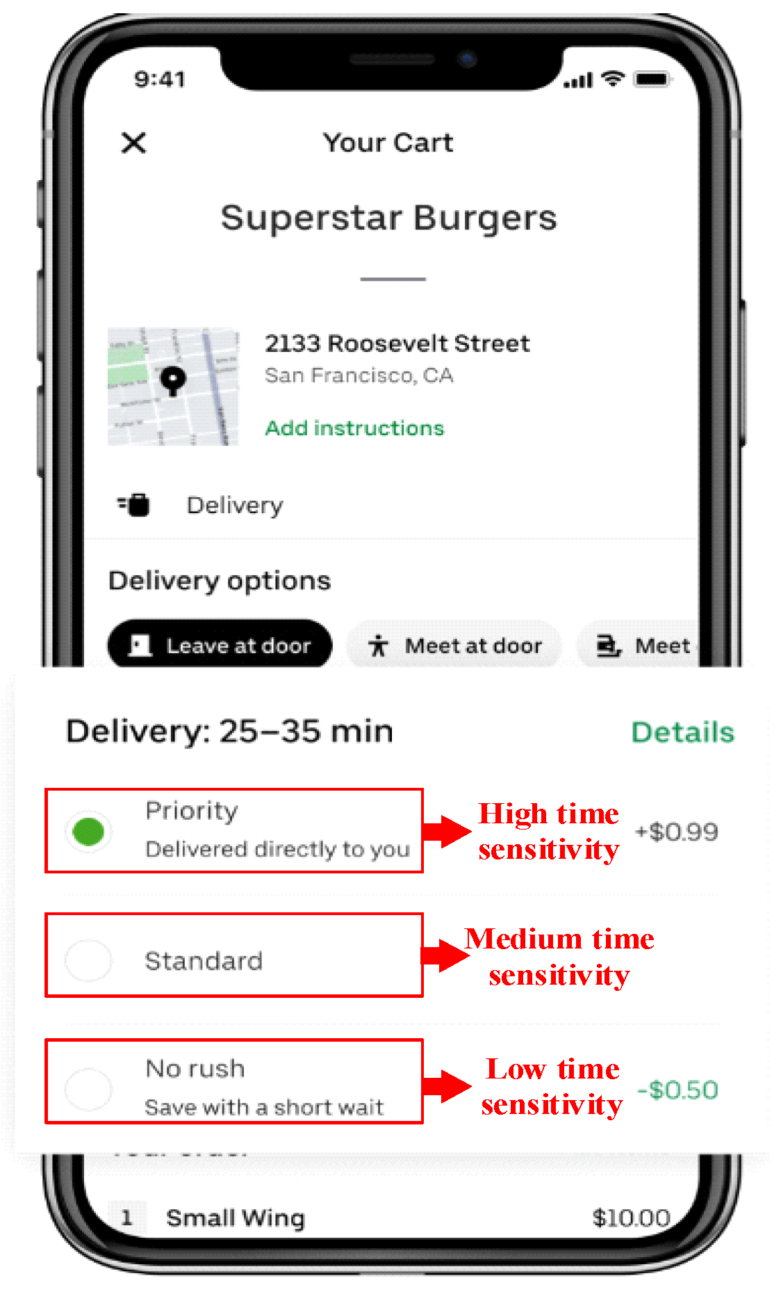
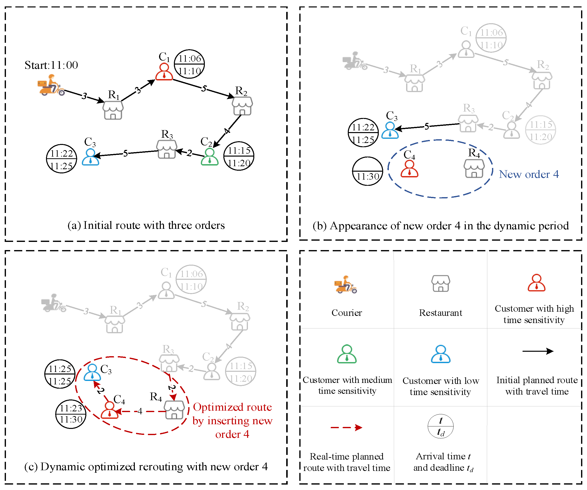
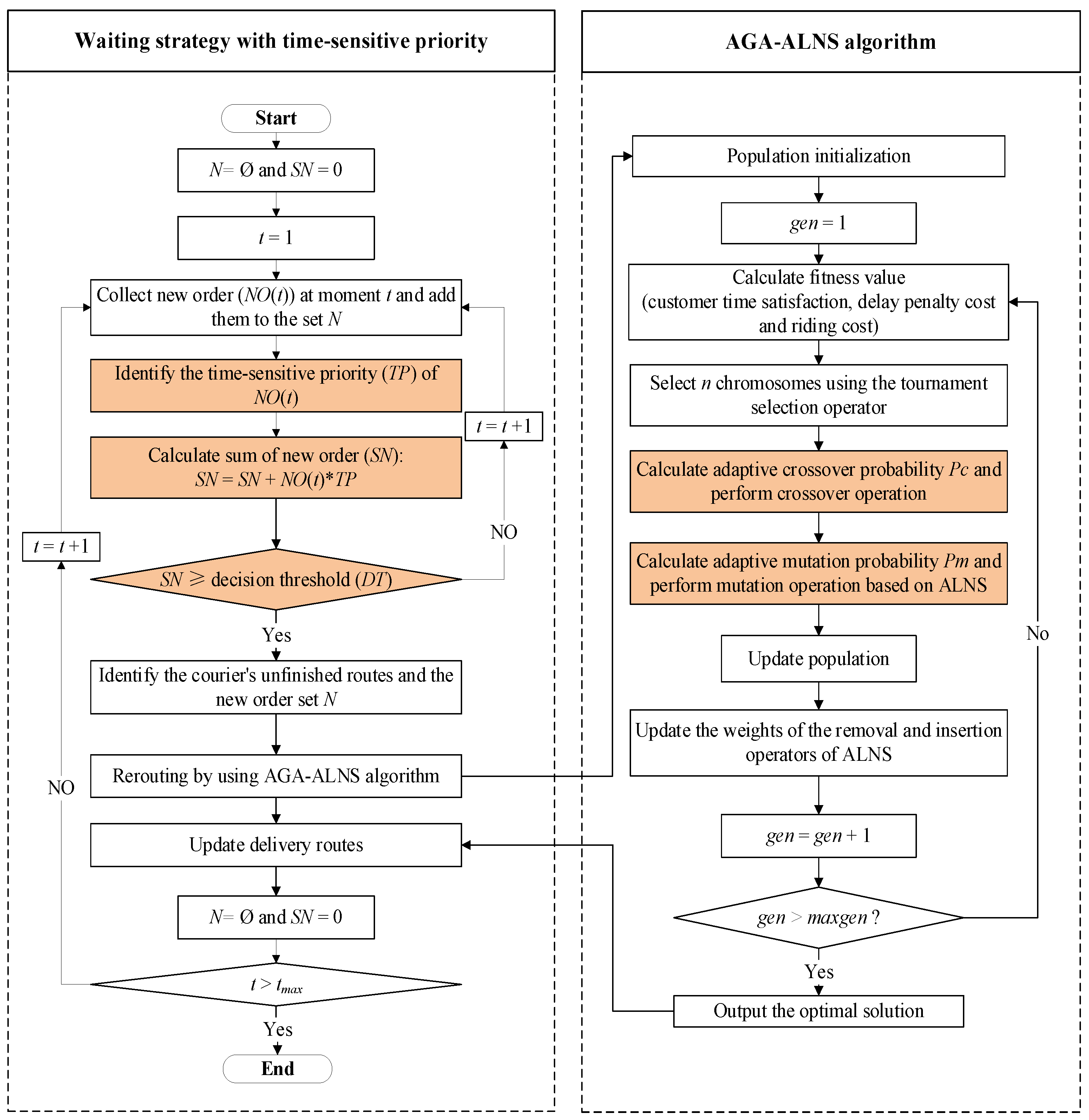
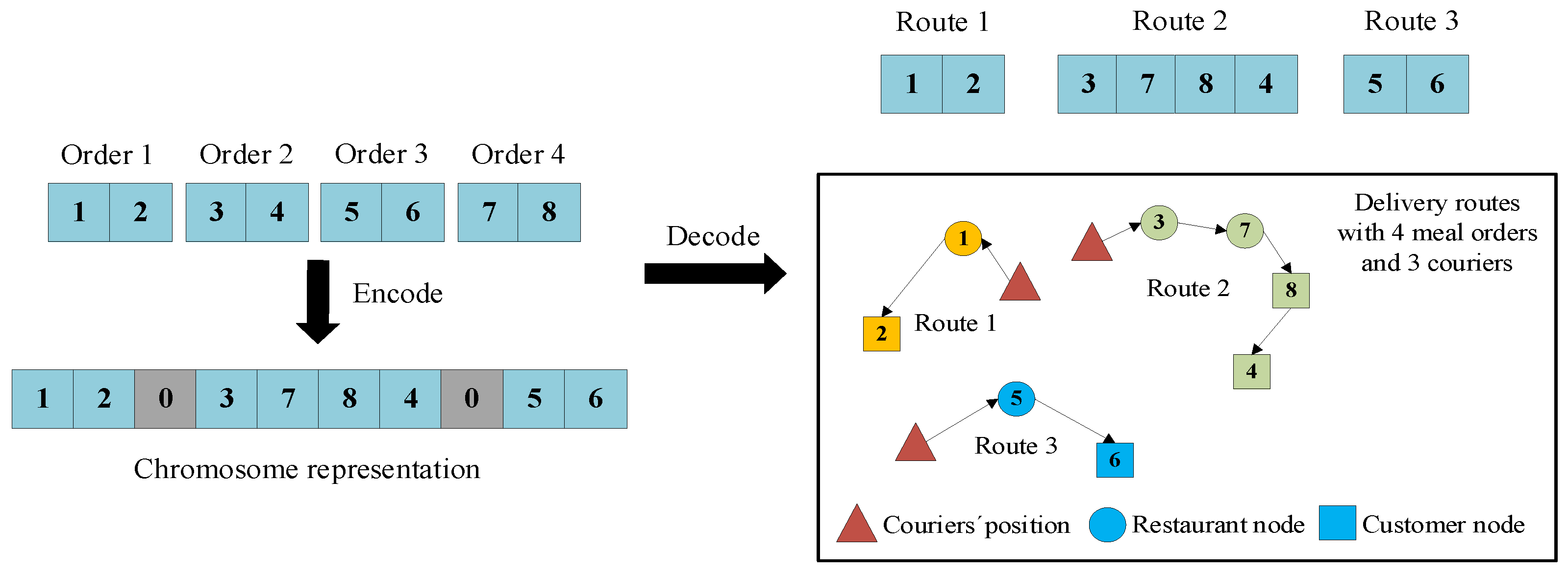
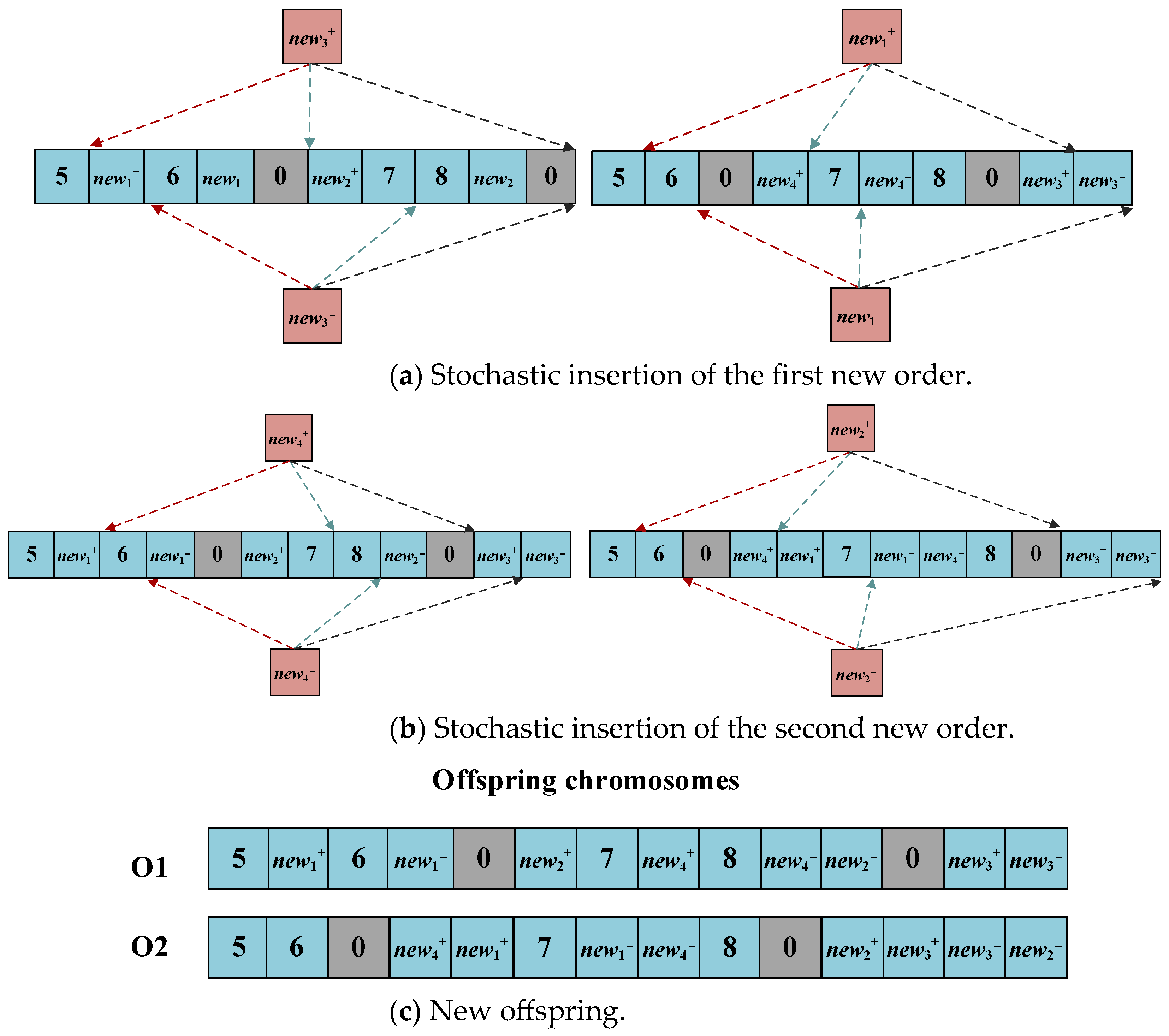
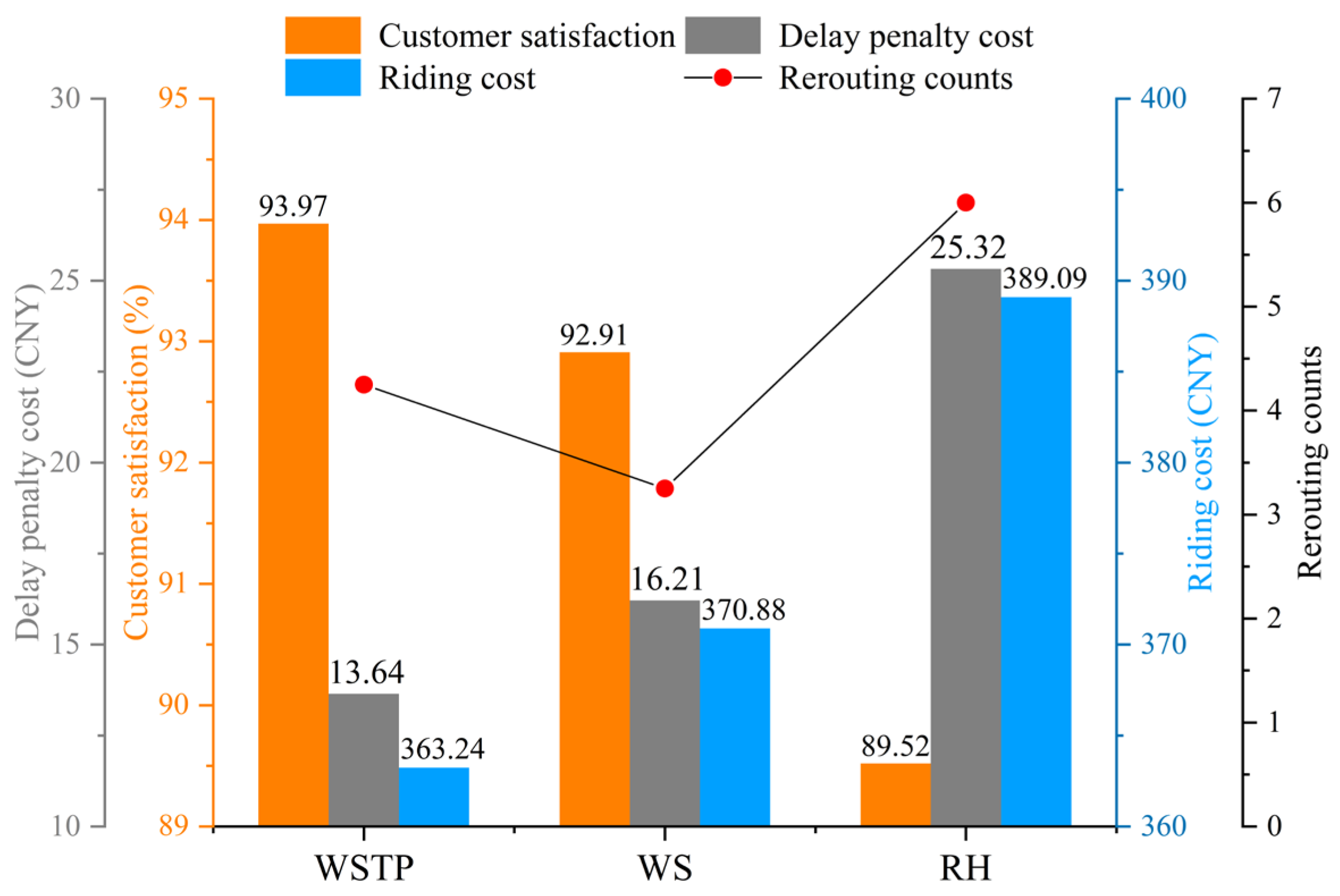
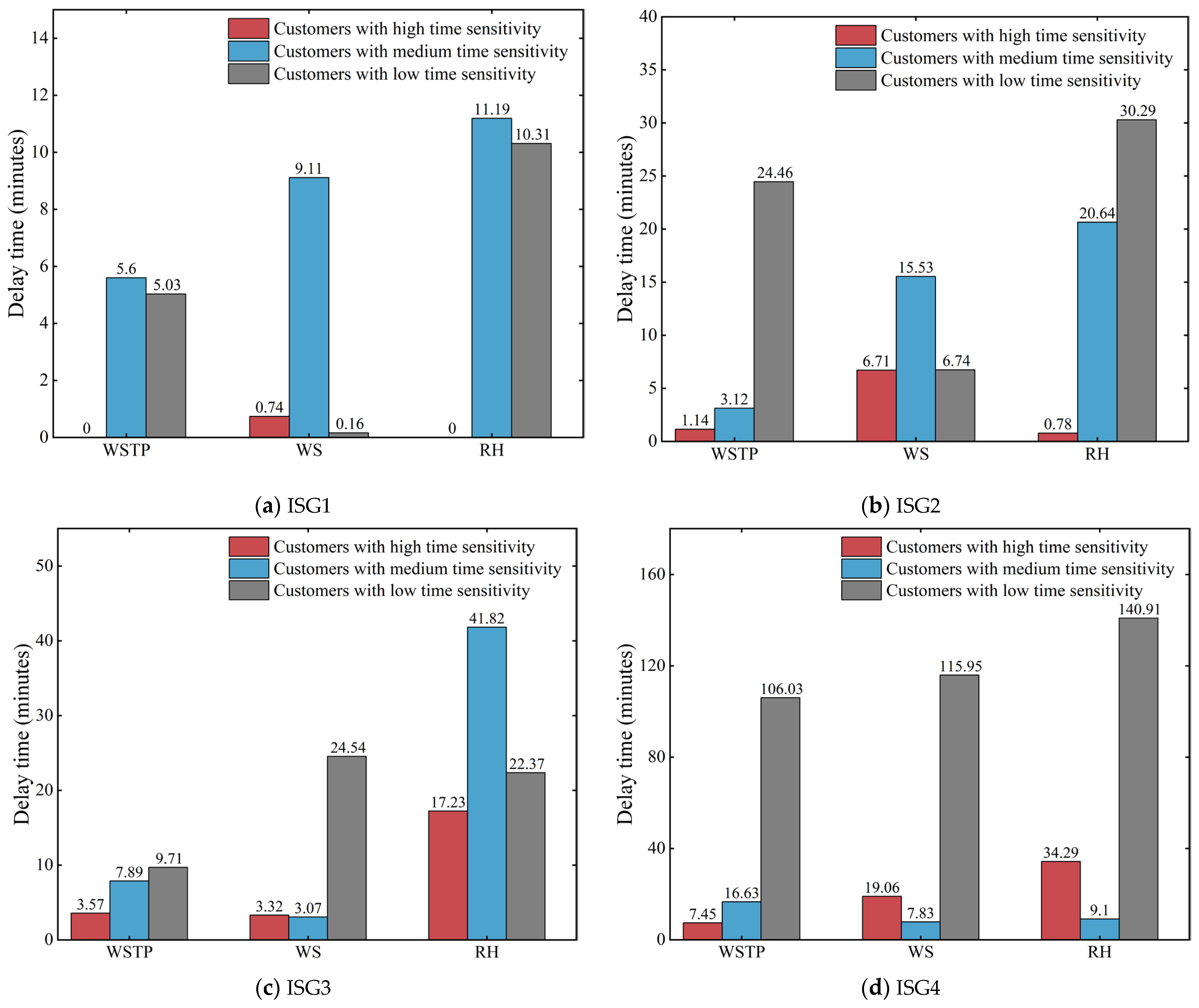
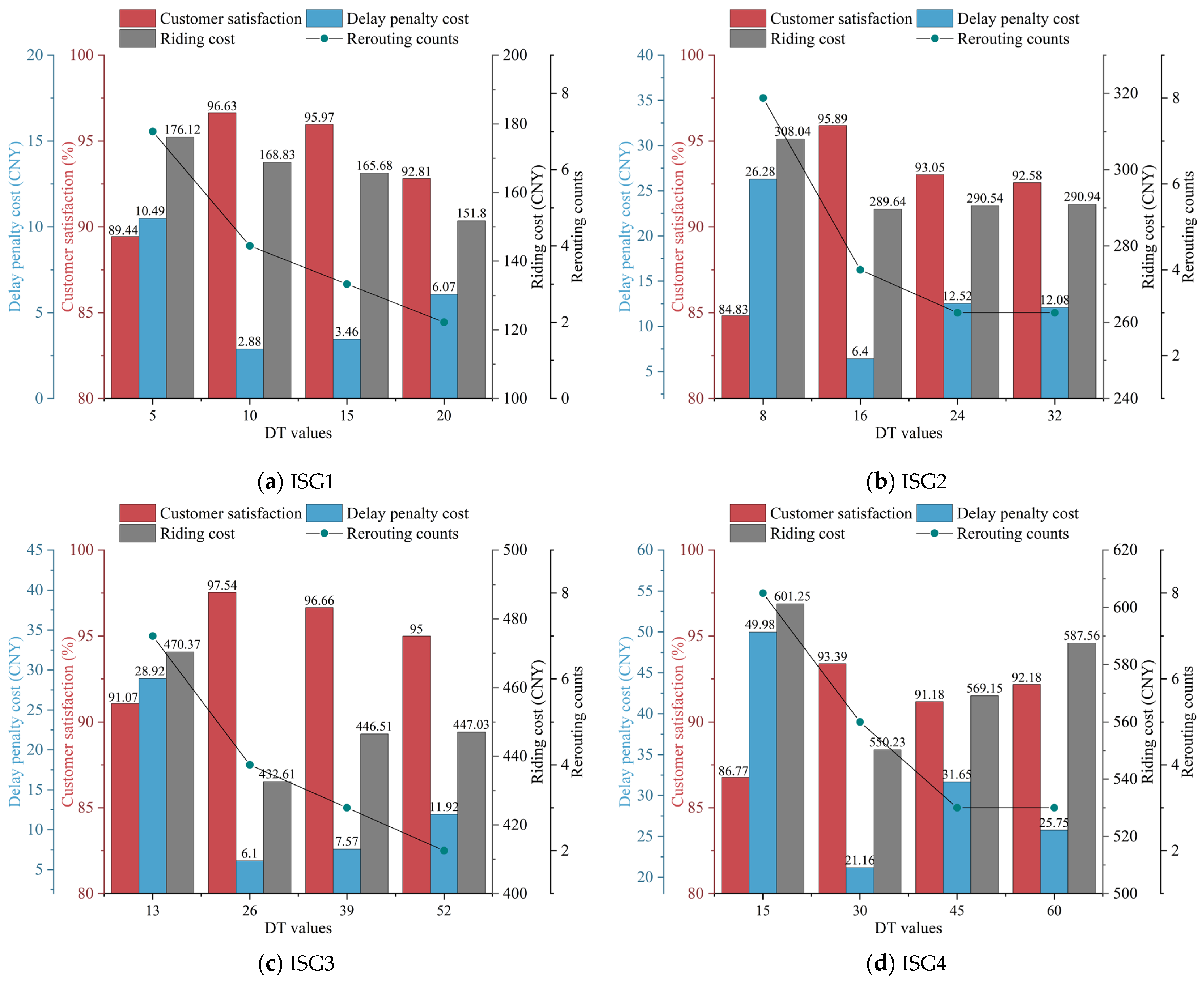
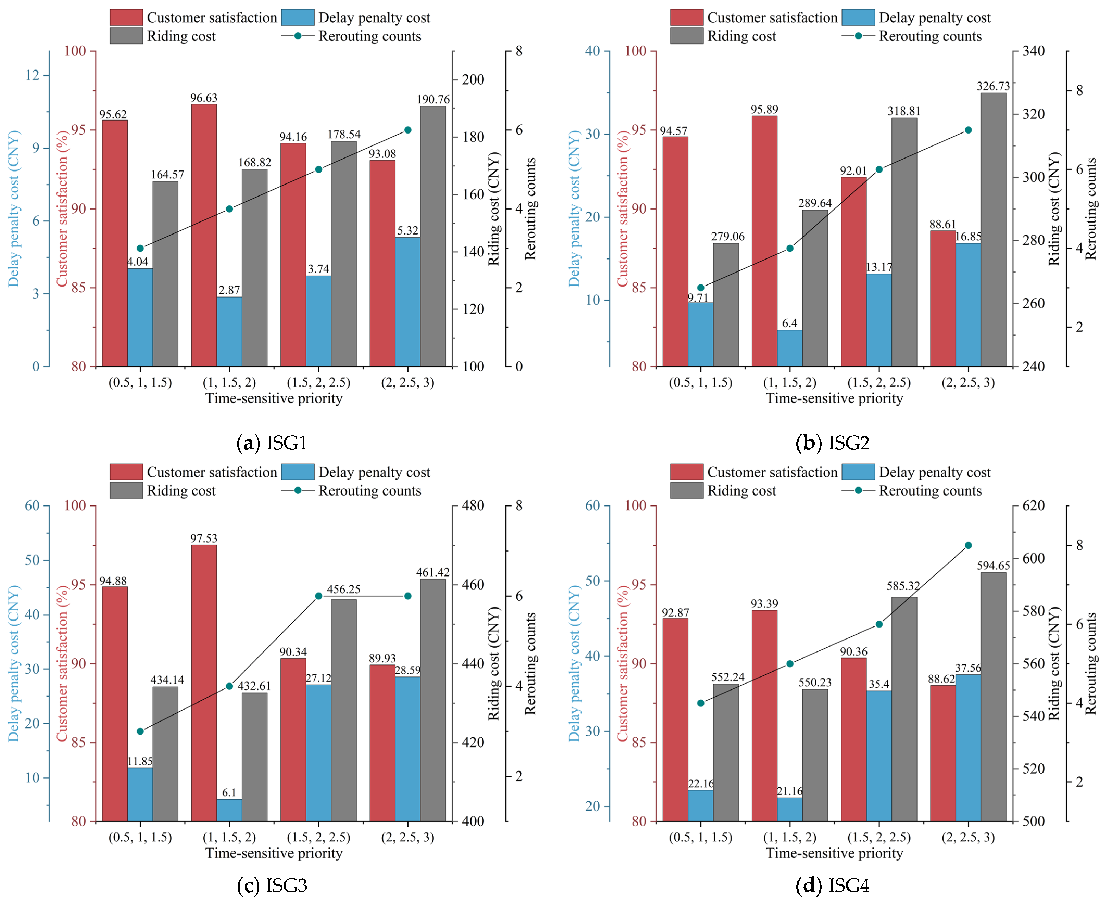
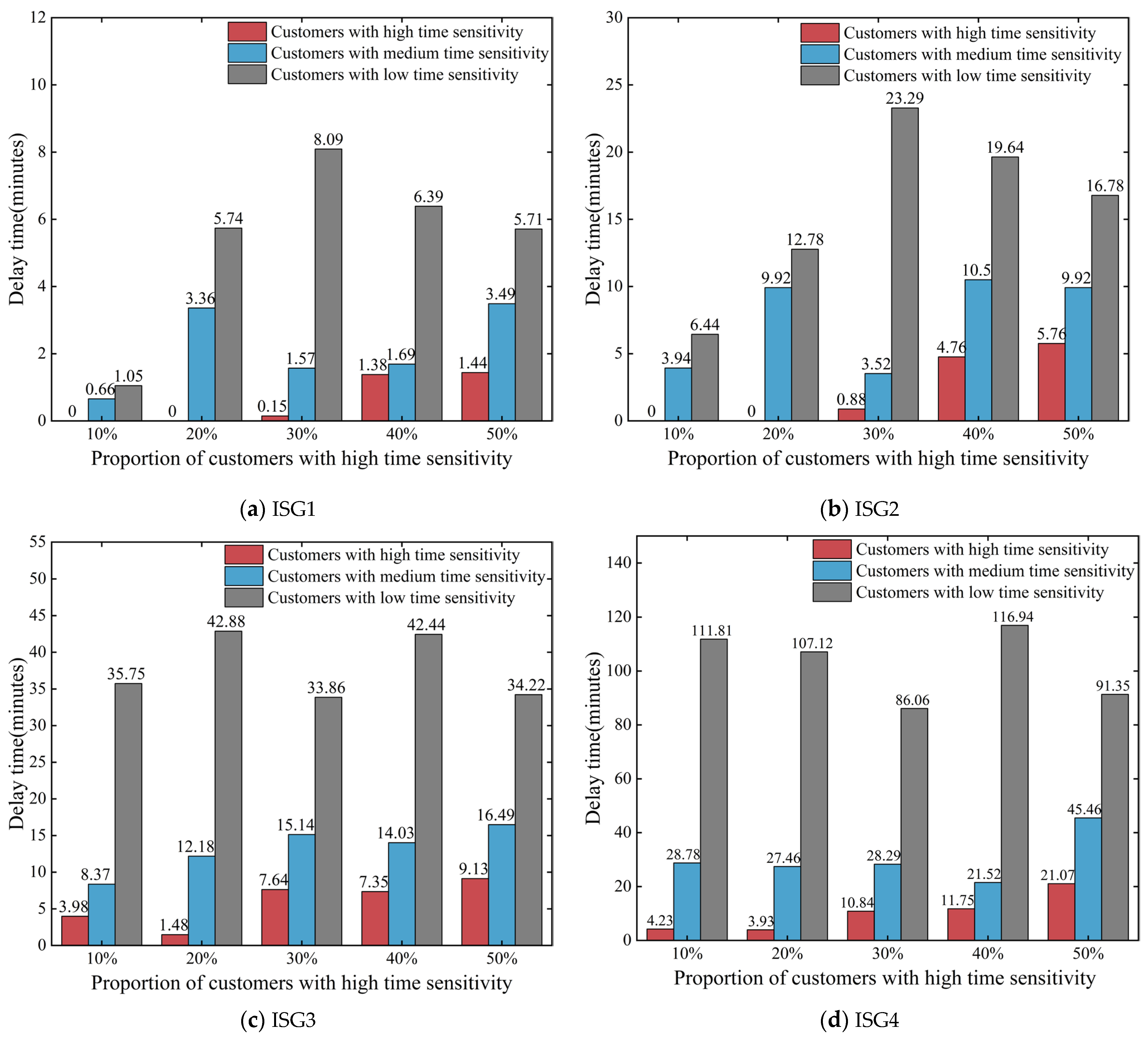