Bootstrap Method of Eco-Efficiency in the Brazilian Agricultural Industry

Abstract

With the economic growth of the Brazilian agroindustry, it is necessary to evaluate the efficiency of this activity in relation to environmental demands for the country’s economic, social, and sustainable development. Within this perspective, the present research aims to examine the eco-efficiency of agricultural production in Brazilian regions, covering 5563 municipalities in the north, northeast, center-west, southeast, and south regions, using data from 2016–2017. In this sense, this study uses the DEA methods (classical and stochastic) and the computational bootstrap method to remove outliers and measure eco-efficiency. The findings lead to two fundamental conclusions: first, by emulating the benchmarks, it is feasible to increase annual revenue and preserved areas to an aggregated regional level by 20.84% while maintaining the same inputs. Given that no municipality has reached an eco-efficiency value equal to 1, there is room for optimization and improvement of production and greater sustainable development of the municipalities. Secondly, climatic factors notably influence eco-efficiency scores, suggesting that increasing temperatures and decreasing precipitation can positively impact eco-efficiency in the region. These conclusions, dependent on regional characteristics, offer valuable information for policymakers to design strategies that balance economic growth and environmental preservation. Furthermore, adaptive policies and measures can be implemented to increase the resilience of local producers and reduce vulnerability to changing climate conditions.

1. Introduction

According to the 2017 Agribusiness Census of the Brazilian Institute of Geography and Statistics (IBGE), more than 15 million people work in agricultural activities, and approximately 5 million establishments are focused on agricultural activities. As a contributor to the country’s financial multiplier effect, agriculture is responsible for a considerable portion of the Brazilian GDP.

Since the sixteenth century, for example, the activity of producing sugar cane for export and the production of cattle to subsidize the agricultural activity in the period shows that, since the early days of colonization, agriculture and cattle ranching were present in the Brazilian economic formation. It is not surprising that more than 638 million tons of sugar cane were produced in 2017, followed by the production of more than 100 million tons of soybeans and 88 million tons of corn. Together, it totals approximately 351 million hectares (3.5 million km²) dedicated to agriculture and cattle ranching, which represents approximately 41% of the national territory [1].

However, the growth of Brazilian agribusiness has led the country to record high levels of deforestation. Cattle ranching activities, for example, have led to this process to generate pastures, which can often lead to land conflicts and forest fires, especially in regions considered the most remote in the country, such as the Amazon [2]. Deforestation causes biodiversity loss, ecosystem deterioration, and increased greenhouse gas emissions. Therefore, if, on the one hand, the economic activity of farming boosts the national economy and food security, and on the other hand, the environmental degradation caused by this activity causes damage to the environment, it is necessary to look for ways to maximize agricultural production and simultaneously minimize environmental degradation, that is, optimize eco-efficiency. This was also a concern raised by [3] regarding sustainable economic development, which has required companies in the agricultural sector to have a competitive advantage in this dynamic environment. Thus, the guiding questions of this work are as follows: (1) Is it possible in Brazil to increase production with fewer resources and environmental impacts? (2) To what extent can agriculture be more eco-efficient?

The search for robust answers to these questions is justified for two reasons. First, the results should provide new practical contributions to support the definition of strategies and actions that harmonize economic growth and environmental preservation, supporting the country’s sustainable agriculture and cattle ranching development. The present study indicates improvements for more eco-efficient agriculture. Second, the literature review shows that this work focuses on a theme that has been little explored in Brazil. Few researchers and research groups deal with eco-efficiency in Brazilian agriculture and cattle ranching, as reflected in the few studies published in relevant scientific journals. Thus, as far as we know, the scientific merits of this research are in its originality.

This is important given the immensity of agricultural activities in the country; there is a greater focus on large producers when referring to sustainable development or eco-efficiency. However, understanding the reality of small producers is paramount because it is not clear whether their activities are sustainable, given the large number of small producers in a country that cause relevant impacts on the performance of the country [4].

The impacts that this economic activity has caused in the country are understood, both positively (financial, job generation, and trade balance) and negatively (land exploitation, deforestation, and waste production). Finding a balance between economic development and environmental preservation is one of the prerogatives of eco-efficiency. It seeks to provide a product to meet human needs, considering the reduction of environmental impacts and optimization to minimize resources to produce more products so that eco-efficiency can be regarded as a practical tool of great importance for the sustainable development of the country [5].

Therefore, this research aims to answer all these questions, including identifying which municipalities and regions are considered eco-efficient and highlighting them as a benchmark for optimizing other municipalities and increasing the country’s eco-efficiency. This will allow a balance between increasing productivity without harming the environment, as well as highlighting which cities and regions need to improve their scores and analyzing whether small producer municipalities can be as eco-efficient as large producers to show that the country, by promoting political and incentive changes, can be as productive and preserve nature in its entirety.

2. Theoretical Methodological Framework

2.1. Literature Review

Making Data Envelopment Analysis (DEA) is a useful tool for this type of analysis. There are two classical models, the CRS model proposed by [6] and the VRS model proposed by [7], based on constant and variable returns to scale, respectively. The CRS and VRS models have advantages and disadvantages; however, several variations have emerged in recent years with increasingly accurate results, thus improving DEA [8].

The literature has various applications of the DEA model in eco-efficiency analysis. Some studies use more straightforward approaches with the application of classic DEA models, such as the measurement of the eco-efficiency of farms in Poland evaluated with a VRS [4] approach and the evaluation of industrial eco-efficiency in urban metropolis areas in Korea, 2000–2015, by the classic CRS and VRS [9] models. Other studies use an individual approach with super-efficiency, as in the case of the analysis of the eco-efficiency of China’s mining system [8] and a gap approach to the super-efficiency model to calculate the eco-efficiency of China’s provinces considering time series with economic, energy, and environmental variables [10,11,12]. We also found another application of a time series to evaluate the evolution of the eco-efficiency of 40 industrial parks using the Malmquist model [13] and a two-stage DEA approach with a random variable Tobit regression analysis to determine industrial eco-efficiency indicators for 30 Chinese provinces from 2005 to 2015 [5]. Other DEA models, which are not commonly applied but which were also used to measure eco-efficiency, were an enhanced DEA model called network DEA (NDEA) to evaluate the eco-efficiency of 30 provinces in China during the period 2003–2016 [14] and the meta frontier framework model, a model that allows maximizing outputs and minimizing inputs at the same time to evaluate the eco-efficiency of 282 European regions from 2006 to 2014 [15].

Bootstrap computational models with DEA are used to evaluate eco-efficiency, and most studies have been conducted in China. The studies include the following: The evaluation of China’s industrial eco-efficiency of 112 resource-based cities from 2003 to 2016 [16], the eco-efficiency of China’s hospitality sector of 31 provinces in the period 2016–2019 [17], analysis of the impact of the Pollution Information Transparency Index (PITI) on the eco-efficiency of 109 cities with environmental protection [18], a study to evaluate the eco-efficiency of the Hungarian agricultural sector [19], the eco-efficiency of 298 Municipal Solid Waste Service Providers (MSWSPs) in Chile [20], an evaluation of the eco-efficiency of 32 municipalities located in Tropical Montane Cloud Forests (TMCF) in Mexico [21,22], the eco-efficiency of municipalities in the Amazon [23], and the regional eco-efficiency in China during 2008–2017 [24]. Thus, several studies focus on evaluating eco-efficiency, but few use bootstrap computational techniques with DEA to remove outliers and calculate eco-efficiency. However, no relevant research looks at agriculture in all Brazilian municipalities, the country’s strongest sector and one of the world’s leading exporters of these products.

2.2. Productivity and Efficiency Models

Based on the studies of [25] on the Measurement of Production Efficiency and [26] on the Economic Theory of Production, the concept of the Production Possibility Set (CPP) is formed given a set of Technologies (T). In this way, considering eco-efficiency, a set of resources will be represented by a vector $\left(x\right)$, given by the area used, the environmental inputs of animals, and plant origin and labor, giving rise to a set of products represented by a vector $\left(y\right)$, containing the positive and negative externalities given by revenue, undesirable outputs, preserved areas, and the diversity index, where T will be given by $(x,y)$. Thus, mathematically, this technological set for calculating eco-efficiency is represented by $T=(x,y)$, where x can produce y.

In this way, given a set of Decision-Making Units ($DM{U}_k$) and their respective inputs and outputs $(x,y)$, a space, $R^{p+q}$, will be structured, given by $\epsilon$$\left(R^q\right)$, and the space of the Technological Frontier (TF) or Efficiency Frontier (F) will be constituted, given by a linear segment that connects each efficient $DM{U}_s$. Below this frontier will be located the inefficient $DM{U}_k$, presenting the need to improve the inputs and outputs of the production process [25]. Therefore, the distance between the frontier given by TF and $DM{U}_k$ represents the optimization needed to make $DM{U}_k$ equally efficient to other $DM{U}_s$, which is called the benchmark [26,27,28].

This is how the eco-efficiency index can be measured, considering the x inputs and y outputs of farming activities and economic, environmental, and social factors, by optimizing the variables, maximizing the outputs, and minimizing the inputs of the production process through what [25] called technical efficiency.

2.3. Eco-Efficiency DEA Model

Based on the study and concept of productivity [25], the first Data Envelopment Analysis (DEA) model was proposed for analyzing the technical efficiency of decision-making units (DMUs), known as the CRS model [6]. The CRS model considers constant returns to scale, i.e., variations in the productive frontier of input and output occur at a steady rate [6]. However, most industrial processes do not exhibit this behavior, and the relationships between inputs and outputs vary, consolidating the second classic DEA model, VRS [7,27].

The DEA model is fundamental to evaluate eco-efficiency (based on Microeconomic Firm Theory), which considers inputs and outputs of different natures, such as economic, environmental, and social. This model allows efficiency to be evaluated by combining variables with varying units of measurement, allowing a quantitative analysis of these variables. It starts by generating more outputs with a smaller amount of input, making the DMU more efficient [8].

The indicators that measure eco-efficiency take into account a desirable economic measure, aligned with the input of some environmental measure in the process; this is because economic growth is always aligned with increased environmental degradation, being necessary a set of technologies and legislations applicable to the process to allow an innovative and sustainable growth with the lowest possible ecological impacts [15].

Going back to the idea of [29], where efficiency is achieved when the DMU has quantities of inputs and outputs that cannot be improved without simultaneously worsening the other, as well as when based on the performance of other DMUs, there are no improvements that can be made without negatively affecting the inputs and outputs. Therefore, eco-efficiency can only be achieved when the use of resources is minimized without increasing the environmental impacts of agro-industrial activities (emission of polluting gases, deforestation of woods and forests, or monoculture).

Therefore, a set of inputs, $X_i$, can produce a set of outputs, $Q_j$; however, maximizing these outputs will not always be a strict eco-efficiency objective because the variable $Q_j$ takes into consideration positive externalities and undesirable outputs, the latter generally related to environmental impacts caused by industrial activities. Then, X can produce $(Q_{\mathrm{desirable}},Q_{\mathrm{undesirable}})$. To solve this problem of maximizing undesirable outputs, one can treat $Y_{\mathrm{undesirable}}$ as the inverse of its original value. Then, X can produce $(Q_{\mathrm{desirable}},\frac{1}{Q_{\mathrm{undesirable}}})$. Thus, when the linear model maximizes outputs, it minimizes undesirable outputs. Thus, eco-efficiency is calculated as a Linear Programming Problem (LPP) identical to the efficiency models described as a constant scale model with output orientation defined by Equation (1):

$$\min \phi \sum _{i=1}^n{V}_i{X}_i+V_0,\sum _{j=1}^m{W}_j{Q}_{jk}=1,\forall r,\sum {j=1}^m{W}_j{Q}_{jr}-\sum _{i=1}^n{V}_i{X}_{ir}+V_0\le 0,\forall r,W_j,V_i\ge 0,\forall j,i$$

(1)

Consider ${\widehat{\theta }}_{CRS}$ and ${\widehat{\phi }}_{CRS}$ the input-oriented and output-oriented eco-efficiency of the CRS model. ${\widehat{\theta }}_{VRS}$ and ${\widehat{\phi }}_{VRS}$ represent the input-oriented and output-oriented eco-efficiency of the VRS model. One has a similar interpretation of the CRS model that ${\widehat{\theta }}_{CRS}=\frac{1}{{\widehat{\phi }}_{CRS}}$; however, due to the orientation of the VRS model, one has that ${\widehat{\theta }}_{VRS}\ne \frac{1}{{\widehat{\phi }}_{VRS}}$. Thus, the eco-efficiency of the VRS model will always be higher than that of the CRS model, caused by a larger number of eco-efficient DMUs in the VRS model than in the CRS model.

Shannon–Weaver Diversity Index

One of the very important variables for calculating eco-efficiency is the Shannon–Weaver Diversity Index (SWDI), which captures the environmental impacts of monoculture. According to [30], the diversity index can be calculated as follows:

$$IDSW=e^{-{\sum }_{c=1}^C{P}_{cr}\ast ln\left(P_{cr}\right)},$$

(2)

where $P_{cr}$ represents the total proportion, P, of the municipalities, r, that is dedicated to culture, c. In this way, the index will have a value from 0 to 1, that is, when the value of the index is equal to 1 it points out a monoculture activity, which is an activity that wears out the soil; therefore, the inverse of this value was made because it is an undesirable output, $1/IDSW$, to calculate eco-efficiency.

3. DEA-Stochastic Model

3.1. Outlier Detection

Because it is a deterministic measure, DEA is extremely sensitive to the presence of outliers to calculate punctual efficiency values, and removal is necessary to avoid skewing the result. The reasons for the presence of outliers in the data can be explained by three main factors: (i) data errors during the process of publishing or collecting the data, (ii) atypical correct values caused by extreme induction, (iii) exceptional values, which perform relatively considerably below, or above, most of the data [31].

The bootstrap concept was introduced by [32], then [33,34] introduced the descriptive methods to identify data influence for non-parametric computation. These methods allow the use of statistical inference without compromising the non-parametric nature of the problem; however, it requires manual work, which often makes it impractical due to the amount and diversity of data handled, as in the case of this research (5563 observations, 5 inputs, and 4 outputs). The use of these methods would bring a disadvantage in their use [35].

To identify outliers, an alternative is to use a cloud methodology, where for each matrix $\left(M\right)$ of parameters n and p, each $DM{U}_i$ (each point) is removed from the space ${\mathbb{R}}^n$ and ${\mathbb{R}}^p$, where the volume $\left(V\right)$ is recalculated by removing the $DM{U}_i$ from the matrix, generating a new volume $V_i$, then calculating the ratio $\left(R\right)$ between V and $V_i$, given by $R_i=V_i/V$, where R will be close to 1 if the value of $V_i$ does not change significantly, so when there is an outlier there will be an R value significantly lower than 1 [31].

Therefore, ref. [36] proposed a new model that combines bootstrap (stochastic model) and Jackknife resampling (deterministic model) for detecting these outliers, where, for each DMU, the efficiency scores of all other DMUs are calculated, the observed DMU is removed, and discrepant outlier values are detected and can either be removed automatically or manually (being a feasible number) from the database.

The author describes some steps for applying the methodology, organized into seven steps:

• First, an algorithm is implemented based on the Jackknife resampling technique. Randomly choose approximately 10% of the set r with $(r=1,\dots ,p)$ to form a subset that we will call t with $(t=1,\dots ,p)$.
• Calculate the efficiencies of the DMUs by the DEA of $\widehat{\theta }t$ com $t=1,\dots ,p$.
• Then, one must recalculate each of the efficiencies by removing each of the DMUs ${\widehat{\theta }}_{t,b}$ with $t=1,\dots ,p$ and $t\ne b$, where each $b=1,\dots ,p$ represents the DMU that was removed. Thus, one must calculate the standard deviation ${\varphi }_b$ of ${\widehat{\theta }}_{t,b}$ with respect to ${\widehat{\theta }}_t$:

  $${\sigma }_b=\sqrt{\frac{{\sum }_{t=1,t\ne b}^p({\widehat{\theta }}_{t,b}^{*}-{\widehat{\theta }}_t)}{p-1}}.$$

  (3)
• Repeat (1, 2, and 3) S times, accumulating the leverage information in ${\theta }_{bs}$, where $n_b=St/p$.
• The average leverage (a value that measures the impact of removing the DMU from the set, given by the standard deviation) is calculated for each DMU. The idea is that outliers will exhibit behavior with a higher leverage than the average of the other DMUs, so it will be selected with a lower probability, where ${\overline{\sigma }}_b={\sum }_{s=1}^{n_b}{\sigma }_{bs}/n_b$.
• Posteriorly, the overall leverage is calculated by summing the average leverage of each DMU, where $\overline{\sigma }={\sum }_{b=1}^p{\overline{\sigma }}_b/p$.
• After Jackknife resampling, bootstrap is applied to insert confidence intervals and information by leveraging to reduce the probability of choosing outliers for stochastic resampling samples; the probability is calculated based on the Heaviside function. In this way, the DMU with a considerable leverage value for overall leverage is discarded.

3.2. Statistical Inference of DEA-Stochastic with Bootstrap

According to [21], another problem of the classic DEA models is their deterministic nature, causing point values to be considered the efficiency estimation without taking into account the uncertainties of the problem values caused by possible noise in the model used and imprecision involving the efficiency estimation. One way to address the problem would be to use statistical inference techniques within the eco-efficiency model to complement the analysis, bringing more robust results by defining confidence intervals, hypothesis testing, and correlating the variables involved, bringing greater reliability and acceptance of the scores resulting from the DEA model. This model, known as stochastic DEA, is based on bootstrap techniques.

The concept of the bootstrap was introduced by [32]. Still, its application with the DEA model was only presented by [37], where the bootstrap simulates a sample with the application of the original estimator, making the simulation results replicate the original sample through a Process of Data Generation (PGD), in a process of resampling, repeated several times. This is somewhat complex when estimating a non-parametric frontier, a set of variables that can have errors and inferences, considering that the inputs and outputs are random variables made up of a little-known data generation process. The model is based on five steps for its application:

• For each observation of the original sample $(x_i,q_i),i=1,\dots ,p$, the DEA corresponding to each $DM{U}_i$ of the original sample represented by ${\widehat{\theta }}_{CRS}$ or ${\widehat{\theta }}_{VRS}$ is calculated (given the result of the scale backtest, the model is represented by ${\widehat{\theta }}_i$).
• Through a resampling process, a set of data is randomly drawn from the original sample. The bootstrap method is used to generate this random sample from the original sample of size p, which corresponds to the eco-efficiency scores, ${\theta }_r,$ with $r=1,\dots ,p$, providing a distribution of a population estimated by the resampling process bootstrap ${\theta }_1^{*},\dots ,{\theta }_p^{*}$.
• From this random sample, we have the inputs and outputs generated in the resampling $X^{*}=[x_1^{*},\dots ,x_p^{*}]$, $Q^{*}=[q_1^{*},\dots ,q_p^{*}]$, $x_r^{*}=\left(\frac{{\widehat{\theta }}_r}{{\theta }_r^{*}}\right)x_r,r=1,\dots ,p$.
• We calculate the estimated bootstrap for the eco-efficiency scores for each $DM{U}_r$ given the values from step (III) ${\widehat{\theta }}_{(i,b)}^{*}$ of i for $i=1,\dots ,p$, via a Linear Programming Problem (LPP) with DEA constraints:

  $${\widehat{\theta }}_{(i,b)}^{*}=min\left\{\theta \mid \sum _{r=1}^p{\lambda }_r{X}_{i,b}^{*}\le \theta x_{io},\sum _{r=1}^p{\lambda }_r{Q}_{mr}\ge q_{mo}\forall m,\sum _{r=1}^p{\lambda }_r=1,{\lambda }_r\ge 0,\forall r\right\}$$

  (4)
  Equation (4) is input-oriented. The output-oriented model follows the same logic.
• We repeat steps (II) to (IV) B times (by default, $B=1000$) to obtain the result with the confidence interval of 95%, given each observation $i=1,\dots ,p$, in a set of estimates, where $\{{\widehat{\theta }}_{i,b}^{*},b=1,\dots ,B\}$.

3.3. Test of the Return to Scale Model

According to [38], it is of strict importance to understand the nature of the behavior of the return to scale for the correct application of the analysis model (CRS, OR VRS) because errors can occur in the analysis due to the distortion of the result due to the type of return, causing a loss of statistical efficiency. Therefore, testing the observations’ behavior is necessary to identify the Technological Frontier (F) behavior. $H_0$ is defined as the F with constant returns to scale and $H_1$ as the F with variable returns to scale.

We calculate each DMU’s efficiency using the CRS and VRS models to define whether the hypothesis is null. Thus, we define the scale efficiency $\left({\widehat{\theta }}_E\right)$ as follows: ${\widehat{\theta }}_E={\widehat{\theta }}_{CRS}/{\widehat{\theta }}_{VRS}$, where ${\widehat{\theta }}_E\le 1$.

If ${\widehat{\theta }}_E$ is approximately equal to 1, this indicates that DMU L has a Constant Returns to Scale (CER) behavior, and the efficiency analysis can be done using the CRS model (${\widehat{\theta }}_{CRS}$). If ${\widehat{\theta }}_E$ is significantly smaller than 1, this indicates that DMU L has Variable Returns to Scale (VRS) behavior, and efficiency analysis should be done using the VRS model (${\widehat{\theta }}_{VRS}$). One then has that $H_0$ is ${\widehat{\theta }}_E=1$, with F being RCC, and $H_1$ is ${\widehat{\theta }}_E<1$, with F is VRS.

The authors of [38] propose that scale efficiency can be calculated as follows: ${\widehat{\theta }}_E={\sum }_{r=1}^p{\widehat{\theta }}_{r,CRS}/{\sum }_{r=1}^p{\widehat{\theta }}_{r,VRS}$.

To define whether ${\widehat{\theta }}_E$ is significantly smaller than 1, the critical value $C_{\alpha }$ is calculated, where if ${\widehat{\theta }}_E>C_{\alpha }$, $H_0$ is accepted. The authors propose using the bootstrap method, with the help of the R function boot.sw98, using the FEAR package; in this way, one can accept $H_0$, provided that $H_a$ is accepted, and calculate the estimated value of ${\widehat{\theta }}_E$ and the critical value $C_{\alpha }$. If $H_a$ is defined as ${\widehat{\theta }}_E$ greater than $C_{\alpha }$, the model is CRS, and if $H_b$ is defined as ${\widehat{\theta }}_E$ less than $C_{\alpha }$, the model is VRS.

Therefore, even if ${\widehat{\theta }}_E$ is less than 1, the model is considered to be CRS by accepting $H_a$, if ${\widehat{\theta }}_E$ is not significantly smaller than 1.

4. Analysis Variables

The research has as a prerogative the analysis of the Brazilian Municipalities through the Data Envelopment Analysis (DEA). This totals approximately 5563 municipalities from all Brazilian states, plus the Distrito Federal. Subdivided between the northern region (Acre—AC, Amapá—AP, Amazonas—AM, Pará—PA, Rondônia—RO, Roraima—RR, Tocantins—TO), northeast region (Maranhão—MA, Piauí—PI, Ceará—CE, Rio Grande do Norte—RN, Paraíba—PB, Pernambuco—PE, Alagoas—AL, Sergipe—SE, Bahia—BA), mid-western region (Distrito Federal—DF, Goiás—GO, Mato Grosso—MT, Mato Grosso do Sul—MS), southeast region (São Paulo—SP, Rio de Janeiro—RJ, Minas Gerais—MG, Espírito Santo—ES), and southern region (Paraná—PR, Santa Catarina—SC, Rio Grande do Sul—RS).

The data were collected from the Agribusiness Census of the Brazilian Institute of Geography and Statistics [1], in the 2017 Agricultural Census (last published to date) to collect the input variables: $x_1$—Area of establishments (hectares), $x_2$—Annual expenditure on fuels and lubricants (Thousand reais), $x_3$—Annual expenditure on inputs for plant and animal production (Thousand reais), $x_4$—Labor employed in establishments (salaried and family), and $x_5$—Other expenditure (Thousand reais). The desirable output variables were as follows: $y_1$—Annual gross revenue (Thousand reais) and $y_2$—Area of natural and planted woods and forests on farms (hectares). The undesirable output variables were as follows: $y_3$—Annual greenhouse gas emissions from the agricultural sector (tons GWP), taken from the Greenhouse Gas Emissions Estimation System (SEEG), and $y_4$—Shannon–Weaver diversity index, calculated using planting variables [1]. Each variable was collected for all 5563 Brazilian municipalities. The data are summarized in Table 1. Access to the databases used for the calculations is: www.figshare.com/articles/dataset/Analysis_of_the_Eco-efficiency_of_Agriculture_in_Brazilian_Municipalities_Based_on_the_Stochastic-DEA_Model/23703174 (accessed on 5 March 2024).

Table 1. Descriptive statistics of inputs (x) and outputs (y).

Variable	Average	Median	Dev.Pad	Maximum	Minimum
$x_1$	63,147.55	24,480.80	138,808.71	4,810,916.30	0.001000
$x_2$	4264.12	1476.00	17,276.88	1,107,997.00	0.042275
$x_3$	51,104.04	18,329.00	109,730.62	1,740,972.06	34.035800
$x_4$	2715.28	1768.00	2,944.54	48,246.00	0.001000
$x_5$	3509.74	955.00	9881.26	251,959.00	0.001000
$y_1$	88,650.06	41,829.00	172,537.12	3,258,836.00	0.001000
$y_2$	18,222.27	4773.00	49,424.62	1,125,574.00	8.391978
$y_3$	101,297.16	39,154.58	206,618.66	4,485,536.54	40.518500
$y_4$	0.080088	0.074229	0.041666	1.000000	0.017115

5. Results Analysis DEA

The results show the process of removing the outliers with the bootstrap. Then, the confidence intervals are analyzed, and the bootstrap is used to construct these intervals. The type of return to scale of technology (F) was defined to determine which model (CRS or VRS) would be appropriate for analysis, and the eco-efficiencies of the municipalities were computed.

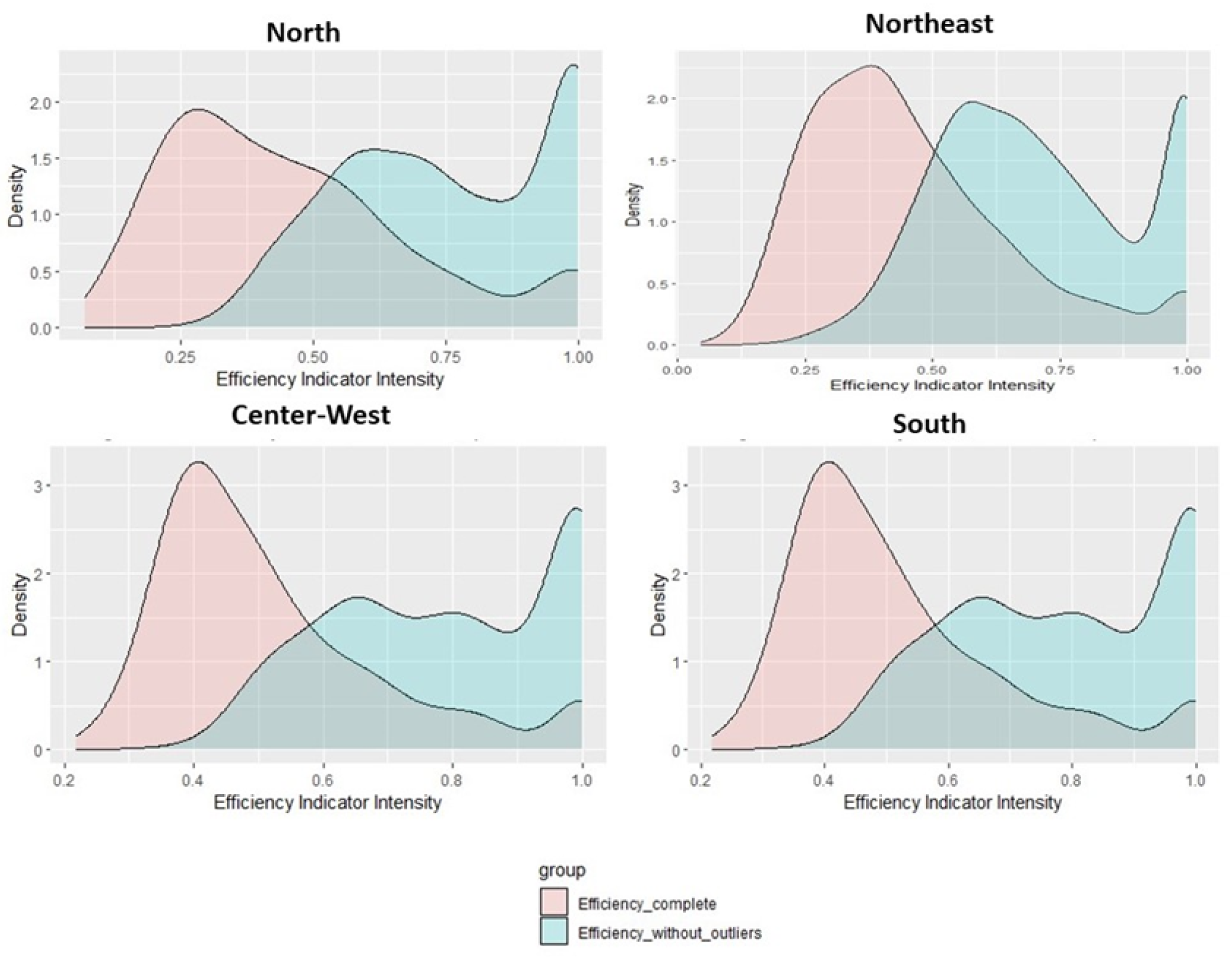
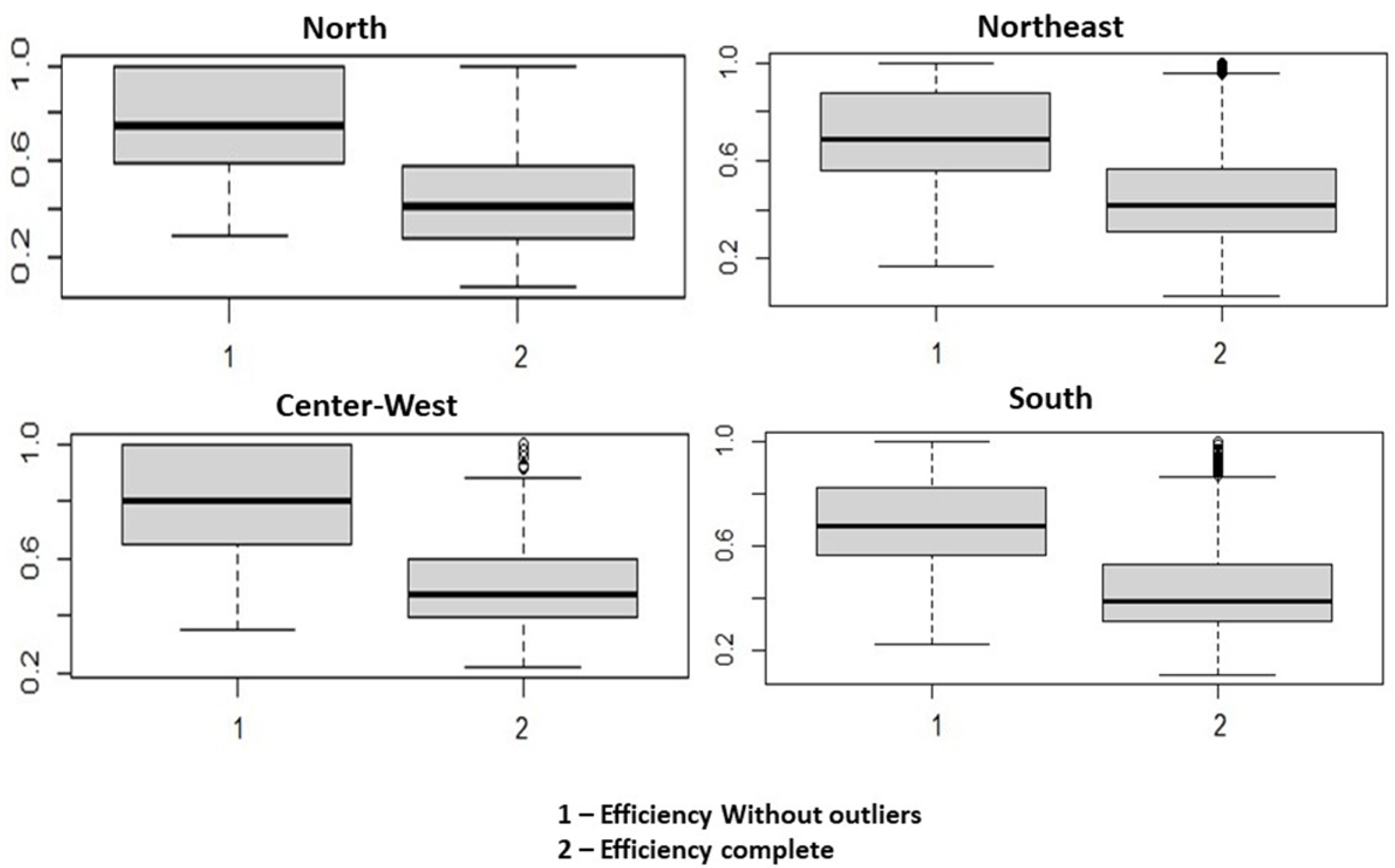
5.1. Removing the Outliers

Because the data can present errors, missing data in the 2017 census (a data protection measure to avoid exposing information certain important properties to third parties) or low homoscedasticity can cause distortions in the results of the DEA analysis or even the heterogeneity of DMUs due to technological differences. Therefore, it is necessary to verify the model’s outliers and remove them so that the result is not biased.

To apply the DEA methodology, the Jackstrap package is used in RStudio to analyze the outliers and apply the bootstrap (available in the R library at: https://cran.r-project.org/web/packages/jackstrap/index.html (accessed on 1 May 2023)), as proposed by Sousa and Monte (2020). With subsets of 10% of the total DMUs to form a subset, t, and the number of repetitions equal to 1000, the average leverage, overall leverage, and withdrawals of the outliers are calculated, according to the steps described in Section 3.2.

As there is a large amount of data, a possible solution is partitioning the data analysis by regions (north, northeast, mid-western, southeast, and south). This simplifies the analysis due to the considerable use of computational processing to remove the outliers in a unified way. The Jackstrap function is used for analysis, with Heaviside and Kolmogorov–Smirnov (K–S) criteria for testing which model has a more satisfactory return. In the southeast region, no outliers are identified for either criterion. Since the Heaviside criterion presented more restricted data, that method was chosen. At the end of the five regions, 143 DMUs were considered outliers. The results are presented in Table 2.

Table 2. Result of outlier removal.

Region	Municipalities	Heaviside	K–S	Municipalities without Outliers
North	450	17	13	433
Northeast	1794	61	21	1733
Mid-Western	467	23	10	444
Southeast	1662	-	-	1662
South	1191	42	21	1149

To understand the influence of outliers on the measurements, the density plots present the frequencies of each region where outliers were found (Figure 1).

Figure 1. Density curves of eco-efficiencies by Region.

Therefore, it is verified that the outliers cause misrepresentation of the data, all biased towards lower eco-efficiency values. The Wilcoxon test comparing the efficiencies with and without outliers found that the mean and median of the two distributions diverged (p-value $<2.2\times {10}^{-16}$, in the regions where outliers were identified). These divergences become more explicit in the boxplots of the efficiencies for each region (Figure 2).

Figure 2. Bloxplots with and without outliers.

As can be seen in Figure 1 and Figure 2, the averages of both graphs are shifted to a lower efficiency score, pulling the eco-efficiencies to a lower performance.

Thus, it is understood that the outliers influence the consistency of the results. Their removal is necessary to analyze the eco-efficiency of the municipalities assertively, resulting in more robust efficiencies. The 143 DMUs removed represent approximately 2.57% of the total, thus consolidating 5420 municipalities for efficiency analysis.

5.2. Scale Return Test

From the new sample resulting from the data without outliers, we can analyze the type of scale return of the data, thus defining which is the best model (CRS or VRS), because the use of any kind of scale return (constant or variable) can generate inadequate results, and it can also cause misrepresentations in the analyses by the evaluation being of a different nature from the real behavior of the sample. As described in Section 3.3, the first hypothesis, $H_0$, is that the technology Frontier (F) has constant returns to scale as long as the scale efficiency, ${\widehat{\theta }}_E$, is equal to 1 (CRS); the $H_1$ considers that the technology Frontier (F) has variable returns to scale as long as the scale efficiency, ${\widehat{\theta }}_E$, is less than 1 (VRS). Given the alternative hypothesis, $H_a$, we can accept $H_0$ if the estimated value is greater than the critical value $({\widehat{\theta }}_E>C_{\alpha })$.

The output orientation is used because the problem deals with undesirable outputs. It is not attractive to keep the emissions as they are to minimize the resources. Still, it is more appealing to keep the inputs and maximize the outputs, which, in the case of undesirable outputs, will be minimized by the model. The data is not partitioned in this step, so the 5420 municipalities return eco-efficiency scores jointly, with 1000 resamples obtained by bootstrap and $\alpha =0.05$.

The estimated value ${\widehat{\theta }}_E=0.9210$ and the critical value $C_{\alpha }=0.8385$ is calculated. Thus, $H_0$ is accepted and F is considered with Constant Returns to Scale (CRS). Therefore, it is understood that regardless of the size of the farm, it can be eco-efficient. This is a good indication for agricultural production since approximately 89% of farmers own a farm of less than 100 hectares and are responsible for 80% of the rural income.

At first, this may be somewhat difficult to understand, considering that most of the sets analyzed often have variable scale behavior, especially in the private sector when analyzing industry [39]. However, from the results, Brazilian agriculture shows different and constant behavior, which confirms an issue related to the fact that inequality in agriculture does not occur by the size of the properties but by the technological availability of them [40].

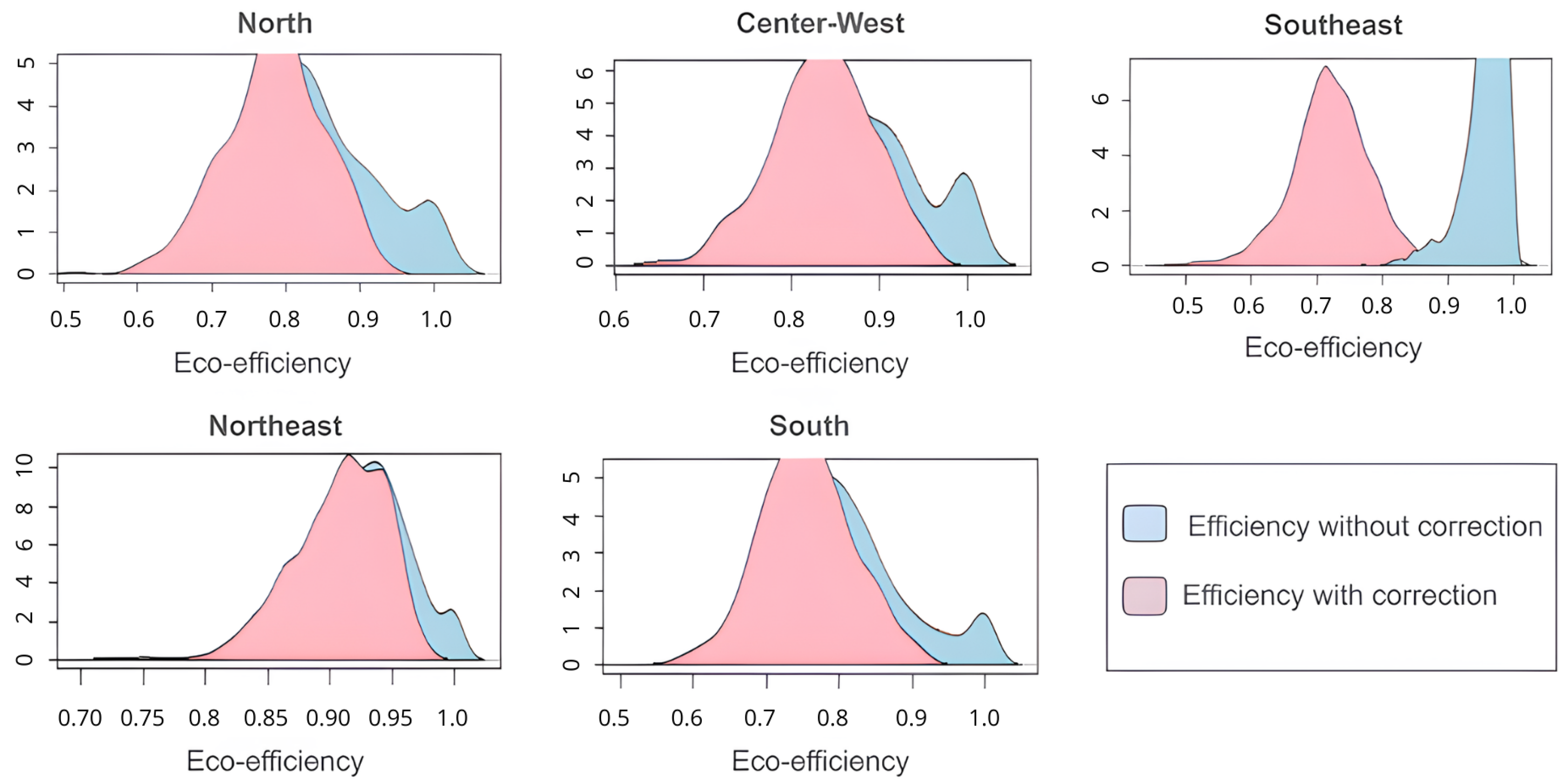
5.3. Statistical Inference of DEA Eco-Efficiency of Municipalities

It is accepted that the technology is CRS and that the production-oriented eco-efficiency indices are estimated. Due to the abundance of data, the analysis is divided into two parts. Table 3 and Table 4 refer to the results of the application of the DEA methodology with bootstrap and the ranking of the best and worst eco-efficiency indices by region, where through the application of the bootstrap the confidence intervals of $\alpha =95\%$ of the eco-efficiency indices of the values (with correction) are structured. Thus, through the methodology adopted, more robust and reliable results were found than the simple application of the classic DEA model (without correction).

Table 3. Ranking of the eco-efficiency index of the best municipalities by region.

Municipalities	Region	Without Outliers with Correction	95% Confidence Interval		Without Outliers without Correction
			Maximun	Minimum
Afuá (PA)	North	0.9340	0.9953	0.9160	1.0000
Presidente Fig. (AM)	North	0.9336	0.9905	0.9130	0.9999
Manaus (AM)	North	0.9295	0.9898	0.8981	0.9999
Porto Walter (AC)	North	0.9195	0.9498	0.8938	0.8620
Pimenta Bueno (RO)	North	0.9150	0.9698	0.8895	0.8346
Araripina (PE)	Northeast	0.9818	0.9914	0.9739	0.7597
Santo Estêvão (BA)	Northeast	0.9814	0.9931	0.9715	0.9499
Macaúbas (BA)	Northeast	0.9806	0.9974	0.9728	0.9474
Itapipoca (CE)	Northeast	0.9792	0.9958	0.9697	0.9736
Iguatu (CE)	Northeast	0.9773	0.9893	0.9683	0.7265
Nova Lacerda (MT)	Center-West	0.9618	0.9947	0.9446	1.000
Ribeirãozinho (MT)	Center-West	0.9533	0.9947	0.9214	0.8420
Inocência (MS)	Center-West	0.9528	0.9952	0.9307	0.6985
Turvânia (GO)	Center-West	0.9520	0.9953	0.9304	0.8385
Edealina (GO)	Center-West	0.9519	0.9888	0.9188	0.7847
Nova Campina (SP)	Southeast	0.9004	0.9261	0.8780	0.6447
Itatinga (SP)	Southeast	0.8888	0.9539	0.8621	0.7763
Cananéia (SP)	Southeast	0.8656	0.9513	0.8467	0.6580
Josenópolis (MG)	Southeast	0.8502	0.9521	0.8321	0.7097
Carbonita (MG)	Southeast	0.8432	0.9732	0.8373	0.6688
Caxias do Sul (RS)	South	0.9400	0.9912	0.9094	0.8493
Giruá (RS)	South	0.9221	0.9663	0.8998	0.8099
Barão do Tri. (RS)	South	0.9174	0.9949	0.9119	0.7158
Mafra (SC)	South	0.9165	0.9755	0.8947	0.8988
Congonhinhas (PR)	South	0.9163	0.9935	0.8976	0.7499

Table 4. Ranking of the eco-efficiency index of the best municipalities by region.

Municipalities	Region	Without Outliers with Correction	95% Confidence Interval		Without Outliers without Correction
			Maximun	Minimum
Aurora do Pará (PA)	North	0.6182	0.6510	0.6056	0.9230
Ariquemes (RO)	North	0.6160	0.6855	0.6001	0.9643
Conceição do A. (PA)	North	0.5986	0.6481	0.5841	0.8317
Rio Sono (TO)	North	0.5962	0.6442	0.5796	0.8541
Amajari (RR)	North	0.5169	0.5786	0.4997	1.0000
Mucugê (BA)	Northeast	0.7354	0.7568	0.7259	0.9841
Aldeias Altas (MA)	Northeast	0.7214	0.7244	0.7179	0.9053
Açailândia (MA)	Northeast	0.7200	0.7573	0.7000	0.9223
Itinga do Mar. (MA)	Northeast	0.7164	0.7410	0.6944	0.9509
Muquém do S.F (BA)	Northeast	0.6867	0.7156	0.6704	0.8742
Antônio João (MS)	Center-West	0.7037	0.7345	0.6882	0.8650
Planaltina (GO)	Center-West	0.6836	0.7204	0.6660	0.8915
Amambai (MS)	Center-West	0.6758	0.6953	0.6581	0.8442
Nova Andradina (MS)	Center-West	0.6474	0.6676	0.6339	0.7609
Nova A. do Sul (MS)	Center-West	0.6447	0.6709	0.6244	0.8676
Jaíba (MG)	Southeast	0.4163	0.4764	0.4191	0.8162
Morro Agudo (SP)	Southeast	0.4139	0.4874	0.4218	0.6971
Paraguaçu Paul. (SP)	Southeast	0.4124	0.4679	0.4043	0.7646
Ecoporanga (ES)	Southeast	0.4105	0.4996	0.4345	0.8066
Ataléia (MG)	Southeast	0.3781	0.4490	0.3981	0.7420
Eldorado do Sul (RS)	South	0.5720	0.6321	0.5583	0.8259
Santo Inácio (PR)	South	0.5667	0.6041	0.5516	0.7305
Iguaraçu (PR)	South	0.5383	0.6088	0.5325	0.8105
Colorado (PR)	South	0.5130	0.5448	0.5016	0.7438
Colorado (RS)	South	0.5130	0.5448	0.5016	0.7530

The municipalities listed in Table 3 are the highest ranked, thus providing valuable information on which municipalities should be considered as benchmarks so that other municipalities can improve their practices in terms of economic and environmental outputs. Table 4 shows which municipalities are in a worrying situation, serving as a reference point for other municipalities to check whether they are close to the least eco-efficient municipalities.

It is verified for the inefficient DMUs that the uncorrected values benefit the eco-efficiency scores, making the inefficient DMUs’ scores higher compared to the corrected scores of the same DMUs. Also, the uncorrected eco-efficiency scores of the efficient DMUs are underestimated; that is, they presented values below the scores with corrected values. One can visualize this difference in the corrected and uncorrected scores in Figure 3.

Figure 3. Region eco-efficiency density chart.

The regions had higher means, medians, and interquartile ranges of the uncorrected data than the corrected data. In this way, the most robust data are obtained. Table 5 contains the descriptive statistics of the efficiencies calculated with outliers, without outliers, and with correction without outliers.

Table 5. Average, median, and range of eco-efficiencies.

Descriptive Statistics			Region
	North	Northeast	Center-West	Southeast	South
Mean with original outlier	0.7343	0.8909	0.6408	0.9589	0.8393
Mean without outlier without correction	0.8355	0.9225	0.8742	0.7265	0.8000
Mean without outliers with correction	0.7839	0.9067	0.8348	0.6802	0.7526
Median with original outlier	0.7571	0.8912	0.6259	0.9661	0.8428
Median without outlier without correction	0.8250	0.9253	0.8649	0.7228	0.7894
Median without outliers with correction	0.7881	0.9125	0.8359	0.6915	0.7526
Amplitude with original outlier	0.2801	0.0650	0.2317	0.0309	0.1112
Amplitude without outlier without correction	0.0529	0.0380	0.0918	0.0753	0.1027
Amplitude without outlier with correction	0.0838	0.0532	0.0761	0.0829	0.0864

Given the average eco-efficiency of the results from the corrected data for the north, northeast, center-west, southeast, and south regions of 0.7839, 0.9067, 0.8348, 0.6802, and 0.7526, respectively, it indicates a possibility for the municipalities of improvements of 21.62%, 9.33%, 16.52%, 31.98%, and 24.74% from each region, which results in an average increase of 20.84% of gross revenue and natural area on farms. There is a decrease in greenhouse gas emissions from the agricultural sector and Shannon–Weaver diversity index, with an average value of 20.84%.

Thus, it is verified that the removal of the outliers, the parameterization of the data, and the correction of the data generate more robust efficiency scores, thus bringing the results closer to the reality of each municipality and Brazilian region.

There is an analysis to define which region has the most eco-efficient municipalities; however, it would be unfair to compare the region that has the most eco-efficient municipalities, given that some regions have more than twice as many municipalities as other regions. One way is to compare eco-efficiency oriented to output and the selection of the five best DMUs in each Region.

In the comparison of the ten best municipalities, it is verified that the southeast, south, and north regions were the ones that came out best, respectively. The northeast and mid-western regions (which did not appear among the ten best municipalities in Table 6) had the worst performance.

Table 6. Eco-efficiency of the top-ten municipalities.

Municipalities	Region	Without Outliers with Correction	95% Confidence Interval		Without Outliers without Correction
			Maximun	Minimum
Araripina (PE)	Northeast	0.9818	0.9914	0.9739	0.9660
Santo Estêvão (BA)	Northeast	0.9814	0.9931	0.9715	0.9569
Macaúbas (BA)	Northeast	0.9806	0.9974	0.9728	0.9849
Itapipoca (CE)	Northeast	0.9792	0.9958	0.9697	0.9933
Iguatu (CE)	Northeast	0.9773	0.9893	0.9683	0.9703
Nova Lacerda (MT)	Mid-West	0.9618	0.9947	0.9446	0.9894
Ribeirãozinho (MT)	Mid-West	0.9533	0.9947	0.9214	0.8947
Inocência (MS)	Mid-West	0.9528	0.9952	0.9307	0.9087
Turvânia (GO)	Mid-West	0.9520	0.9953	0.9304	0.8886
Edealina (GO)	Mid-West	0.9519	0.9888	0.9188	0.8639

Regarding the best-placed municipalities, the values with corrections presented values above the uncorrected scores, and some DMUs presented values above the corrected score. By the confidence interval, we can differentiate the eco-efficiency among these units. Thus, a confidence interval for the scores is defined.

The overall average of the municipalities is 0.7891 (value without outliers and with confidence bias), which is different from the regional averages of the eco-efficiency index of the north (0.7839), northeast (0.9067), center-west (0.8348), southeast (0.6802), and south (0.7526) regions. An interesting point of the regional averages is that the northeast region presents, on average, higher score values than all regions, which shows that the region, despite having few eco-efficient municipalities, is closer to the productive frontier compared to other regions; this shows a greater homogeneity between the areas of agricultural activity in the region.

The southeast and the south have the lowest averages per region of 0.6802 and 0.7526, respectively, below the general average, which shows that the municipalities that are not part of the productive frontier of these regions are more distant from the eco-efficient frontier, pointing to a greater heterogeneity between the areas of agricultural activity in the region.

This is the case of the Ataléia (MG) municipality, with an eco-efficiency score of 0.3782. Therefore, the southeast and south regions present good performances for some DMUs but also represent the lowest municipal performances.

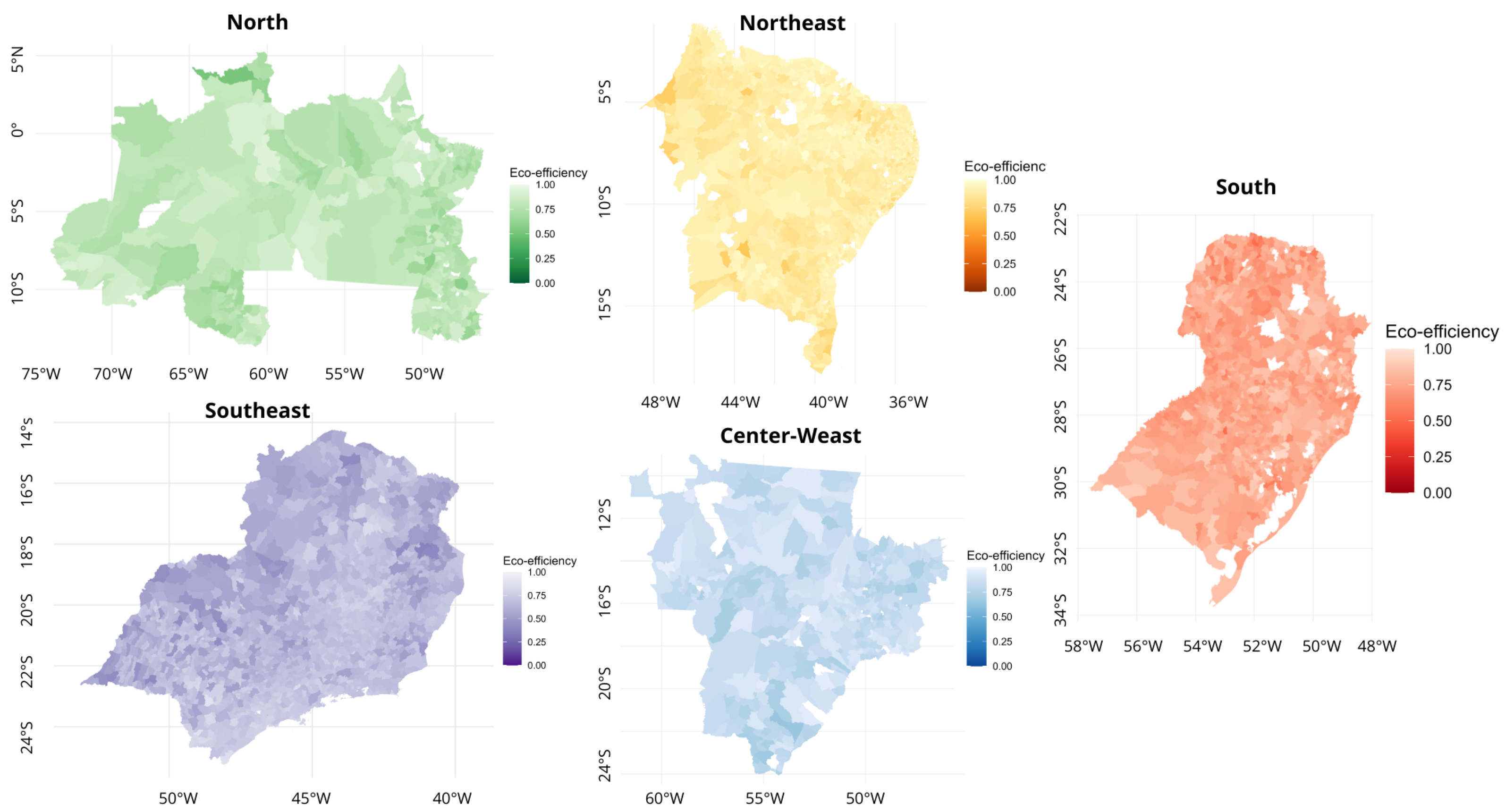
5.4. Geocoding of Eco-Efficiency Score Data in Brazilian Municipalities

Geocoding was used to describe different production and sustainability patterns in municipalities and regions. In this way, the greater the homogeneity between the municipalities of a region, the better distributed the resources and sustainable measures are because the municipalities are equally efficient, as well as pointing to a lesser influence of location on eco-efficiency; thus, in this region, improvements in policies and incentives could occur at the state or regional level, different from the heterogeneous areas, which demonstrate that some municipalities are not very eco-efficient in comparison with neighboring municipalities that have similar resources and conditions in terms of location, climate, and precipitation, among other external factors that can influence production, so policies and tax incentives must be evaluated on a more individual basis for each municipality as they address a local problem.

This can be visualized in the geocoding of eco-efficiency score data in municipalities, generated using the geobr package from RStudio (Available in the R library at https://cran.r-project.org/package=geobr (accessed on 5 March 2024) by Pereira et al. (2022)). It pulls data from IBGE to carry out the geocoding; this way, the scores calculated for eco-efficiency and the geocoding information available from IBGE from 2017 are combined, and the available scale graphs are plotted in Figure 4. The blank sites are the missing municipalities that do not present eco-efficiency scores because they are considered outliers.

Figure 4. Geocoding of eco-efficiency scores per region.

In the north region, the most inefficient DMUs are located in the coastal part and close to the northeast region; as the location moves towards the inner part of the region under analysis, the eco-efficiency scores tend to increase. However, the scale of the map as a whole also shows homogeneity.

In the northeast region, as in the north region, the scores of the most inefficient DMUs are closer to the coast or close to the borders of other states; however, this does not present a significant scale contrast, presenting more homogeneous scores.

In the center-west region, we notice a greater heterogeneity among the scores compared to the north and northeast regions, with a greater contrast among the scales of each municipality. That is, both the efficient and the less efficient DMUs are randomly distributed by the geographic spacing. However, the scale of the municipalities in this region mainly presents scores closer to 1.

In the southeast region, a more excellent contrast is visualized, which points to high heterogeneity in the data between the eco-efficiency score scales and a tendency for the most inefficient DMUs to be located in the border areas of the mid-western and northeast regions. In contrast, efficient DMUs tend to be located in the inner part of the region.

In the south, as in the southeast, the eco-efficiency scores show greater heterogeneity among the municipalities, and the scores tend to be higher in the southern part of the graph.

6. Conclusions

In this work, we use the bootstrap method to verify the model’s outliers and estimate a confidence bias of the efficiencies calculated for 5420 Brazilian municipalities. The Jackstrap package is used to identify and eliminate the outliers that influence the quality of the results. In theory, the DEA model is sensitive to outliers, and this can be proven by the present research, which demonstrates that the outliers cause a shift in the average efficiency scores to lower values compared to the efficiency scores with the presence of outliers. Then, a scale-back test was performed to identify the technology (F) behavior of the model; as a result, the CRS model was obtained to estimate the efficiency scores by means of the boot.sw98 function.

As a result, differences were obtained between the density curves of the efficiency sets of the data with the presence of outliers and the data without outliers for all regions, except for the southeast region, where there are no outliers. This resulted in the elimination of 143 DMUs from the original data set, which shifted the mean of the density curves. This shows that the presence of these outliers biased the results and, therefore, great caution is necessary to interpret results when they are present in the model, highlighting the importance of using bootstrap in the analysis.

The definition of the type of scale return as the CRS model is a relevant result for understanding Brazilian agriculture, where there is a large availability of land distributed heterogeneously (unevenly) among most rural producers because it was found that the small, medium, and large producers can become equally eco-efficient. This becomes more evident when the eco-efficiency scores of the municipalities are calculated, and the critical value is estimated compared to the scale of eco-efficiency. It is analyzed that both large and small producers were considered eco-efficient, which affirms the ability of the small producer to become eco-efficient. However, it is essential to note that most municipalities considered eco-efficient in the analysis were large and medium-sized because they have greater access to technology.

The analysis allows the ranking of the ten most eco-efficient municipalities, these being Araripina (PE), Santo Estêvão (BA), Macaúbas (BA), Itapipoca (CE), Iguatu (CE), Nova Lacerda (MT), Ribeirãozinho (MT), Inocência (MS), Turvânia (GO), and Edealina (GO), respectively, with highlights for the northeast and mid-western regions, Therefore, through the descriptive statistics and the geocoding of eco-efficiency score maps, it is understood that the regions that present higher eco-efficiency scores in the ranking also show a greater homogeneity in the scores compared to other municipalities in the same area, which highlights that the municipalities in the northeast and mid-western region (better placed in the ranking) are at a closer level for eco-efficiency than in other areas.

Among the municipalities, one looks at the scores calculated with and without correction, analyzes the need to establish a confidence interval for the correct classification of these DMUs, and demonstrates the need to be careful when calculating eco-efficiency scores deterministically, with care in the treatment of the data, removal of the outliers, parameterization of the data, and use of the bootstrap to establish a confidence interval.

As a suggestion for future studies, it would be interesting to add a variable correlated with the country’s consumption of fertilizers to analyze the efficiency of agriculture. There are studies in the European Union on efficiency considering the production of fertilizers [41], given the events of recent years involving the Russian war with Ukraine, which has had an impact on the price of fertilizers for agriculture in Brazil. Therefore, it would be relevant for further research.

Another possible future work is to make estimates without undesirable results and then compare the current scenario with a hypothetical scenario. Given the depth required for this type of analysis, considering the findings presented in the results, it is possible to present questions and insights regarding the improvements that can be made by each municipality, both in terms of financial gains and the reduction of undesirable emissions.

References

- Brazilian Institute of Geography and Statistics. Agricultural Census 2017: Definitive Results, 2017. Available online: https://sidra.ibge.gov.br/pesquisa/censo-agropecuario/censo-agropecuario-2017/resultados-definitivos (accessed on 30 January 2023).
- Hamid, S.S.; Santos, M.A.S.D.; Aguiar, A.F.; Andreatta, T.; Costa, N.L.; Lopes, M.L.B.; Lourenço-Júnior, J.D.B. Changes and Factors Determining the Efficiency of Cattle Farming in the State of Pará, Brazilian Amazon. Sustainability 2023, 15, 10187. [Google Scholar] [CrossRef]
- Bobitan, N.; Dumitrescu, D.; Burca, V. Agriculture’s Efficiency in the Context of Sustainable Agriculture—A Benchmarking Analysis of Financial Performance with Data Envelopment Analysis and Malmquist Index. Sustainability 2023, 15, 12169. [Google Scholar] [CrossRef]
- Stepien, S.; Czyżewski, B.; Sapa, A.; Borychowski, M.; Poczta, W.; Poczta-Wajda, A. Eco-efficiency of small-scale farming in Poland and its institutional drivers. J. Clean. Prod. 2021, 279, 123721. [Google Scholar] [CrossRef]
- Matsumoto, K.; Chen, Y. Industrial eco-efficiency and its determinants in China: A two-stage approach. Ecol. Indic. 2021, 130, 108072. [Google Scholar] [CrossRef]
- Charnes, A.; Cooper, W.W.; Rhodes, E. Measuring the efficiency of decision making units. Eur. J. Oper. Res. 1978, 2, 429–444. [Google Scholar] [CrossRef]
- Banker, R.D.; Charnes, A.; Cooper, W.W. Some models for estimating technical and scale inefficiencies in data envelopment analysis. Manag. Sci. 1984, 30, 1078–1092. [Google Scholar] [CrossRef]
- Liu, X.; Guo, P.; Guo, S. Assessing the eco-efficiency of a circular economy system in China’s coal mining areas: Emergy and data envelopment analysis. J. Clean. Prod. 2019, 206, 1101–1109. [Google Scholar] [CrossRef]
- Shah, I.H.; Dong, L.; Park, H.-S. Tracking urban sustainability transition: An eco-efficiency analysis on eco-industrial development in Ulsan, Korea. J. Clean. Prod. 2020, 262, 121286. [Google Scholar] [CrossRef]
- Huang, J.X.; Yu, J.; Zhang, N. Composite eco-efficiency indicators for China based on data envelopment analysis. Ecol. Indic. 2019, 85, 674–697. [Google Scholar] [CrossRef]
- Yu, Y.; Peng, C.; Li, Y. Do neighboring prefectures matter in promoting eco-efficiency? Empirical evidence from China. Technol. Forecast. Soc. Chang. 2019, 144, 456–465. [Google Scholar] [CrossRef]
- Zhou, C.; Shi, C.; Wang, S.; Zhang, G. Estimation of eco-efficiency and its influencing factors in Guangdong province based on Super-SBM and panel regression models. Ecol. Indic. 2018, 86, 67–80. [Google Scholar] [CrossRef]
- Fan, Y.; Bai, B.; Qiao, Q.; Kang, P.; Zhang, Y.; Guo, J. Study on eco-efficiency of industrial parks in China based on data envelopment analysis. J. Environ. Manag. 2017, 192, 107–115. [Google Scholar] [CrossRef] [PubMed]
- Yu, S.; Liu, J.; Li, L. Evaluating provincial eco-efficiency in China: An improved network data envelopment analysis model with undesirable output. Environ. Sci. Pollut. Res. 2020, 27, 6886–6903. [Google Scholar] [CrossRef] [PubMed]
- Bianchi, M.; Del Valle, I.; Tapia, C. Measuring eco-efficiency in European regions: Evidence from a territorial perspective. J. Clean. Prod. 2020, 276, 123246. [Google Scholar] [CrossRef]
- Chen, Y.; Chen, Y.; Yin, G.; Liu, Y. Industrial eco-efficiency of resource-based cities in China: Spatial–temporal dynamics and associated factors. Environ. Sci. Pollut. Res. 2023, 30, 94436–94454. [Google Scholar] [CrossRef] [PubMed]
- Li, Y.; Liu, A.C.; Yu, Y.Y.; Zhang, Y.; Zhan, Y.; Lin, W.C. Bootstrapped DEA and clustering analysis of eco-Efficiency in China’s hotel industry. Sustainability 2022, 14, 2925. [Google Scholar] [CrossRef]
- Yu, Y.; Huang, J.; Luo, N. Can more environmental information disclosure lead to higher eco-efficiency? Evidence from China. Sustainability 2018, 10, 528. [Google Scholar] [CrossRef]
- Baráth, L.; Bakucs, Z.; Benedek, Z.; Fertő, I.; Nagy, Z.; Vígh, E.; Debrenti, E.; Fogarasi, J. Does participation in agri-environmental schemes increase eco-efficiency? Sci. Total. Environ. 2024, 906, 167518. [Google Scholar] [CrossRef] [PubMed]
- Molinos-Senante, M.; Maziotis, A.; Sala-Garrido, R.; Mocholí-Arce, M. Factors influencing eco-efficiency of municipal solid waste management in Chile: A double-bootstrap approach. Waste Manag. Res. 2023, 41, 457–466. [Google Scholar] [CrossRef] [PubMed]
- Peña, C.R.; Pensado-Leglise, M.D.R.; Serrano, A.L.M.; Bernal-Campos, A.A.; Hernández-Cayetano, M.; Staddon, P.L. Agricultural eco-efficiency and climate determinants: Application of dea with bootstrap methods in the tropical montane cloud forests of Puebla, Mexico. Sustain. Environ. 2022, 8, 2138852. [Google Scholar] [CrossRef]
- Penã, C.R.; Rosano, C.A.; Rodrigues, E.; Serrano, A.L.M. Spatial dependency of eco-efficiency of agriculture in São Paulo. Braz. Bus. Rev. 2020, 17, 328–343. [Google Scholar] [CrossRef]
- da Silva, J.V.B.; Rosano-Peña, C.; Martins, M.M.V.; Tavares, R.C.; da Silva, P.H.B. Eco-efficiency of agricultural production in the Brazilian Amazon: Determinant factors and spatial dependence. Rev. Econ. Sociol. Rural. 2021, 60, 250907. [Google Scholar] [CrossRef]
- Yang, L.; Ma, C.; Yang, Y.; Zhang, E.; Lv, H. Estimating the regional eco-efficiency in China based on bootstrapping by-production technologies. J. Clean. Prod. 2020, 243, 118550. [Google Scholar] [CrossRef]
- Farrell, M.J. The measurement of productive efficiency. J. R. Stat. Soc. 1957, 120, 253–281. [Google Scholar] [CrossRef]
- Shephard, R.W. The Theory of Cost and Production Function; Princeton University Press: Princeton, NJ, USA, 1970; p. 308. [Google Scholar]
- Peña, C.R.; Guarnieri, P.; Sobreiro, V.A.; Serrano, A.L.M.; Kimura, H. A measure of sustainability of Brazilian agribusiness using directional distance functions and data envelopment analysis. Int. J. Sustain. Dev. World Ecol. 2014, 21, 210–222. [Google Scholar] [CrossRef]
- Peña, C.R.; Serrano, A.L.M.; Britto, P.A.P.; Franco, V.R.; Guarnieri, P.; Karim, T. Environmental preservation costs and eco-efficiency in Amazonian agriculture: Application of hyperbolic distance functions. J. Clean. Prod. 2018, 197, 699–707. [Google Scholar] [CrossRef]
- Koopmans, T.C. Analysis of production as an efficient combination of activities. In Activity Analysis of Production and Allocation Proceedings of a Conference; Koopmans, T.C., Alchian, A., Dantizg, G.B., Georgescu-Roegen, N., Samuelson, P.A., Tucker, A.W., Eds.; John Wiley and Sons: New York, NY, USA, 1951; Volume 13, p. 33e97. [Google Scholar] [CrossRef][Green Version]
- Beltrán-Esteve, M.; Gómez-Limón, J.A.; Picazo-Tadeo, A.J. Assessing the impact of agri-environmental schemes on the eco-efficiency of rain-fed agriculture. Span. J. Agric. Res. 2012, 10, 911–925. [Google Scholar] [CrossRef]
- Bogetoft, P.; Otto, L. Benchmarking with dea, sfa, and r; Springer Science & Business Media: Berlin/Heidelberg, Germany, 2011. [Google Scholar]
- Efron, B. Bootstrap methods: Another look at the jackknife. Ann. Stat. 1979, 7, 1–26. [Google Scholar] [CrossRef]
- Wilson, P. Detecting Influential Observations in Data Envelopment Analysis. J. Product. Anal. 1993, 6, 27–45. [Google Scholar] [CrossRef]
- Wilson, P. Detecting Influential Observations in Deterministic Non-Parametric Frontiers Models. J. Bus. Econ. Stat. 1995, 11, 319–323. [Google Scholar] [CrossRef]
- Stošić, B.D. Technical Efficiency of the Brazilian Municipalities: Correcting nonparametric frontier measurements for outliers. J. Product. Anal. 2005, 24, 157–181. [Google Scholar]
- Stošić, B.D. Jackstrapping DEA scores for robust efficiency measurement. An. XXV Encontro Bras. Econom. SBE 2003, 23, 1525–1540. [Google Scholar]
- Simar, L.; Wilson, P.W. Sensitivity analysis of efficiency scores: How to bootstrap in nonparametric frontier models. Manag. Sci. 1998, 44, 49–61. [Google Scholar] [CrossRef]
- Simar, L.; Wilson, P.W. Non-parametric tests of returns to scale. Eur. J. 2002, 139, 115–132. [Google Scholar] [CrossRef]
- Yang, L.; Ouyang, H.; Fang, K.; Ye, L.; Zhang, J. Evaluation of regional environmental efficiencies in China based on super-efficiency-DEA. Ecol. Indic. 2015, 51, 13–19. [Google Scholar] [CrossRef]
- Da Silva, G.S.E.; Gomes, E.G. A stochastic production frontier analysis of the Brazilian agriculture in the presence of an endogenous covariate. In Proceedings of the Operations Research and Enterprise Systems: 7th International Conference, ICORES 2018, Funchal, Madeira, Portugal, 24–26 January 2018; Revised Selected Papers 7. Springer International Publishing: Berlin/Heidelberg, Germany, 2019; pp. 3–14. [Google Scholar]
- Radlińska, K. Some Theoretical and Practical Aspects of Technical Efficiency—The Example of European Union Agriculture. Sustainability 2023, 15, 13509. [Google Scholar] [CrossRef]
Disclaimer/Publisher’s Note: The statements, opinions and data contained in all publications are solely those of the individual author(s) and contributor(s) and not of MDPI and/or the editor(s). MDPI and/or the editor(s) disclaim responsibility for any injury to people or property resulting from any ideas, methods, instructions or products referred to in the content. |
© 2024 by the authors. Licensee MDPI, Basel, Switzerland. This article is an open access article distributed under the terms and conditions of the Creative Commons Attribution (CC BY) license (https://creativecommons.org/licenses/by/4.0/).