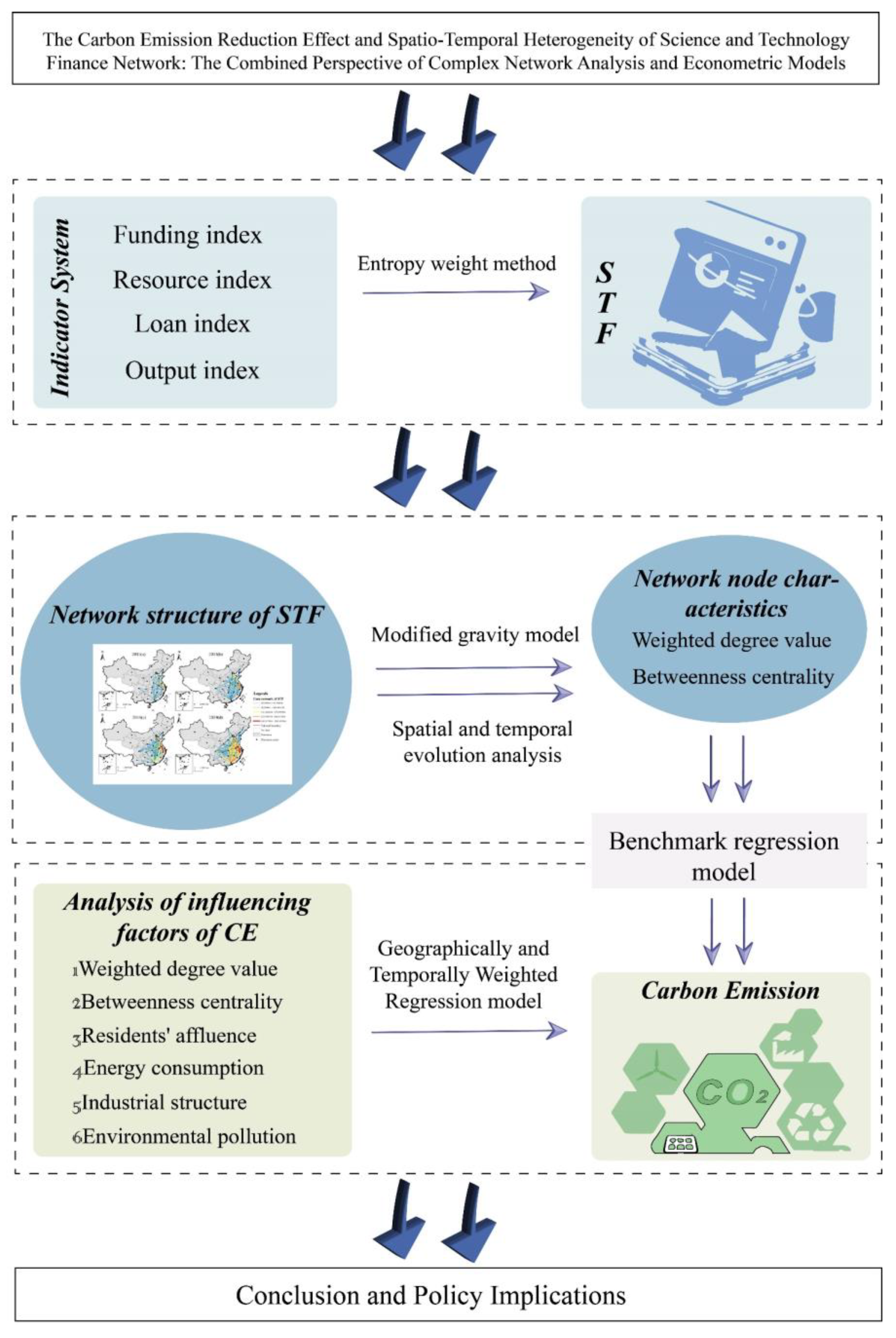
The Carbon Emission Reduction Effect and Spatio-Temporal Heterogeneity of the Science and Technology Finance Network: The Combined Perspective of Complex Network Analysis and Econometric Models

Abstract

With the active promotion of the “carbon peaking and carbon neutrality” goals, science and technology finance (STF) is the important driving force of low-carbon development, and financial networks facilitate the aggregation and transformation of resources in space, so it is of great theoretical and practical significance to investigate the impact of science and technology finance networks (STFN) on carbon emissions (CE). Based on the 30 provinces of China from 2011 to 2019, this article used the STF development level in each province as the main indicator to construct the STFN. The complex network analysis and econometric models are combined, with the weighted degree values and betweenness centrality selected as typical network structure indicators incorporating into the econometric model to explore their impact on CE. Then, the Geographically and Temporally Weighted Regression (GTWR) model is applied to analyse the spatio-temporal heterogeneity of influencing factors. The results show the following: (1) From 2011 to 2019, the spatial structure of China’s STFN has changed significantly, and the status of the triangle structure consisting of Beijing–Tianjin–Hebei (BTH)–Yangtze River Delta (YRD)–Pearl River Delta (PRD) is gradually consolidated in the overall network, and the network structure tends to be stable. (2) The results of the benchmark regression show that the weighted degree value of the STFN has a significant inhibitory effect on CE, while betweenness centrality shows a certain positive effect on CE. (3) The weighted degree value has a more significant effect on CE reduction in the eastern region, while the betweenness centrality has a more significant effect on CE reduction in the central and western regions, but shows a significant promotion effect in the eastern region. (4) There is spatio-temporal heterogeneity in the effects of residents’ affluence, energy consumption, industrial structure, and environmental pollution on CE.

1. Introduction

Serious environmental problems such as melting glaciers, rising sea levels, and global warming have become the focus of attention for people around the world, and promoting low-carbon development has become the consensus of all sectors of society. According to the statistical data of the World Energy Statistics Yearbook 2021, from 2011 to 2020, China’s CE has risen from 8.83 billion ton to 9.90 billion ton, accounting for a larger share of the world’s total CE, and the situation of emission reduction is severe [1]. As a responsible country that supports the building of a community with a shared future for mankind, China has made active exploration and practice in facing global climate governance issues. In September 2020, China pledged at the United Nations General Assembly to achieve the goal of “carbon peaking and carbon neutrality” by 2030 and 2060, demonstrating its mission and determination to promote CE reduction. China’s commitment to reduce CE will lay a solid environmental foundation for the sustainable development of humanity.

At present, there are many studies on CE in academia, mainly focusing on the prediction of CE and the analysis of influencing factors. Scholars have mainly used the STIRPAT model and the Logarithmic Mean Divisia Index (LMDI) to conduct quantitative analysis and think that the focus should be on the impact of factors such as population size, economic and social development, and energy consumption on CE [2,3]. Pan and Zhang believe that population size growth will increase energy consumption [4], but when economic development crosses the environmental Kuznets curve’s “inflexion point”, GDP per capita and CE show a negative correlation. Among them, the CE reduction effect of financial development has also been widely explored and studied. Some scholars have measured the level of financial development and investigated the pathways of its impact on CE. For example, Shahbaz et al. discovered through an empirical study that financial development would reduce CE by improving energy use efficiency and technology [5]. Furthermore, Huang et al. used different indicators to measure the level of financial development and found that financial scale and efficiency had significant effects on CE [6]. The influence of STF on CE in a quasi-natural experiment of “promoting the combination of science and technology and finance” regarding the effect of STF on CE in a pilot area has also been investigated [7].

With the development of economic globalisation, the links between countries and individual provinces are gradually strengthening. Factors of production spread and flow in space and resources are absorbed and clustered between different regions, thus forming inter-province networks. Network analysis is an important method for studying urban network relationships, and the characteristics of urban networks it portrays are conducive to the concretisation of urban network research [8,9]. Financial networks are a microscopic portrayal of urban networks attached to the financial industry. Financial networks promote the spatial concentration of financial resources, facilitate the rapid reorganisation and flow of financial capital in the spatial scope, and promote capital accumulation [10]. In 2020, Zhongguancun built China’s first STF innovation centre and strived to realise the effective docking of capital and science and technology. However, current research on STF mainly revolves around STF policies and the efficiency of STF, but there are still relatively few analytical methods using networks [11,12]. With the deepening of research on STF and its role in promoting technological innovation, STF has shown new development trends and gradually presented diverse and complex relationships among various subjects. Therefore, using complex network analysis methods and constructing complex network models to explore the evolutionary development of STFN will be a key direction for future research. Le Li et al. proposed the concept of STFN to study the role of government financial resources in science and technology innovation networks [13]. Yulian Xu and Lang Yu applied the network model to the evolutionary process of STF and analysed the evolutionary characteristics of STFN at different stages [14].

From the above review, it can be found that at present, the academics have conducted a large number of studies on STF, influencing factors of CE, and complex network analysis, etc., but there is still a lack of studies on the construction of STFN based on spatial network association, and the studies on the impact of STF on CE only remains at the level of policy effects and based on the perspective of attribute data, and lacks an in-depth analysis of the relationship between STF linkages among provinces and the resulting complex spatial network on CE from a relational perspective. When the nodes in the network are strongly related to each other, the traditional econometric research method may not be able to measure and draw the real and accurate conclusions, while the advantage of the econometric research method of integrated social network analysis lies in the adoption and analysis of the “relationship data”, which can effectively reveal the association status between the research subjects and can macroscopically grasp their functions and positioning in the network, eliminate the disadvantage of considering only their own attributes and neglecting the interrelated relationships with other subjects when researching the “attribute data”. At present, most studies are based on social and economic indicators such as “attribute data” rather than “relationship data”. “Attribute data” can only describe the attributes, characteristics, and internal states of entities, and the investigation of their impact on other subjects can only reflect the impact of the attribute characteristics, failing to consider the external linkages among entities and ignoring the impact of the spatial network attributes and externalities of interregional economic and financial development [15]. In addition, although relevant studies have also considered the influence of the spatial aggregation or spatial spillover effect of the corresponding indicators, most of them focus on the geographic “proximity relationship” and cannot reflect the global relationship of the spatial network. On the other hand, the “relationship data” generated through the construction of the network can measure the relationships and interactions between different entities and fully consider the “relationship effect” of variables; for instance, the structural characteristics of the technical cooperation transfer network are treated as independent variables to explore its impact on urban innovation capability [16]. The network structure constructed by relationships has its own intrinsic dynamics and logic, although the nodes construct the network structure based on their own attributes; after the construction of the network is completed, the relational attributes may have a stronger reaction, even beyond their own attributes, which is approved by the related research from the University of Pennsylvania [17].

Therefore, the construction of an STFN will help to further analyse the imbalance and complexity of the development of STF in different regions, help to promote the coordinated development of STF in the regions, and help to accurately identify the status and advantages of each province in the overall spatial network. The spatial network structure is not completely synchronised with the level of economic development, science and technology financial development, etc., and the position and function of network nodes in the network have a great impact on the agglomeration and diffusion of resources, and the network structure indicators, such as the weighted degree value, betweenness centrality, etc., can measure the controlling and intermediary roles that nodes play in the network. In this context, it is important to accurately measure the linkages and interactions among provinces in the network space, and to substitute network indicators into the benchmark regression to detect their influence on CE, which can measure the influence of relevant economic and social factors as well as the influence of the network structure of STF. This study on the relationship between the structural characteristics of STFN and CE is of great guiding significance for revealing the differences in the CE reduction effects of STF among regions and improving the unbalanced development of regions, and it is also a reference for the transformation of energy and the industrial structure development of enterprises in corresponding industries, and the adjustment and strategic deployment of economic policies by relevant government departments according to local conditions.

This study enriches the research content in the field of STF and broadens the research scale of CE, which is of theoretical significance for the scientific understanding of the topic of “how the location and function of science and technology finance network nodes affect carbon emission”, and of great practical significance for the promotion of inter-regional carbon emission reduction effect and low-carbon green development. The main contributions and innovations of this article are as follows: firstly, from a micro and relational perspective, we constructed the STFN based on the modified gravity model, adopted the “relationship data” of the spatial network structure, and selected two representative indicators of network structure, namely the weighted degree value and betweenness centrality, as the core explanatory variables to be included in the econometric model to examine their impact on CE. Secondly, based on a GTWR model, the spatio-temporal heterogeneity of the factors influencing CE is explored, and the differences and correlations between different regions in the CE reduction effects of STFN are fully considered. Thirdly, due to the differences in the degree of economic development among different regions, this article explores the spatial evolutionary development of STFN on CE and the relationship between spatial effects from a spatial horizontal perspective, and further elaborates the inner mechanism of the impact of STFN on CE, to provide certain reference suggestions for CE reduction. The inclusive research framework is shown in Figure 1.

2. Mechanism and Research Hypothesis

The weighted degree value measures the core status of a province in the whole network and its ability to gather economic resources. The higher the weighted degree value, the higher the province’s ability to control capital acquisition and technology absorption in the STFN [18]. Therefore, provinces with high weighted degree values tend to have higher levels of economic and technological development, and have more significant advantages in the absorption and transformation of financial capital, human resources, and technological information. Firstly, regions with a high weighted degree value have a higher level of science and technology. By gathering various preferential policies, they promote the accumulation of innovation resources and the improvement of the innovation level, so as to promote the technological progress of enterprises. The improvement of the innovation capacity and the technological progress of enterprises can promote the optimisation and transformation of the industrial structure, reduce the consumption of highly polluting energy, and thus reduce CE [19]. Secondly, regions with high weighted degree values have more diversified financing channels. By building investment and financing platforms for science and technology innovation, providing differentiated financial services, and attracting foreign investment, which can reduce the difficulty and cost of enterprise financing, they improve their financing ability and stimulate their innovation ability, further bring about the optimisation and upgrading of the industrial structure, and help transform and develop the traditional high-consumption and high-pollution production model, reduce energy consumption, and thus reduce CE [20]. Finally, regions with high weighted degree values have a stronger ability to integrate STF resources and optimise resource allocation efficiency [21]. When STF resources are disseminated and flow in an overall network, the effective integration and utilisation of financial and technological resources improve the efficiency of resource utilisation, thus reducing CE. Accordingly, Hypothesis 1 is proposed in this article.

Hypothesis 1. 

Higher weighted degree values of STFN contribute to lower carbon emissions.

Betweenness centrality is a measure of the ratio of the number of shortest paths through a node to other nodes in the overall network space, in which the node acts as a medium of exchange between other provinces. The higher the betweenness centrality value of a province in the network, the greater its role as an exchanger in the network, and the more conducive it is to the dissemination and diffusion of resources such as innovation and technology and human resources [22]. Compared to the weighted degree values, provinces with higher betweenness centrality generally act as “transit points” for the absorption and transformation of resources, and play the function of gathering and dispersing financial capital. With the strengthening of STF links in the overall network space, the acceleration of capital flows between provinces will stimulate consumption, increase investment, and boost economic growth. An affluent financing environment and a buoyant state of the economy provide more convenient conditions for consumers and investors. While regions with economies in transition will expand their production and increase their demand for energy, the effect of this demand on energy and the scale of production will increase energy consumption and thus contribute to CE [23]. Accordingly, this article proposes Hypothesis 2.

Hypothesis 2. 

Higher betweenness centrality of STFN may lead to increased carbon emissions.

Both the weighted degree value and betweenness centrality are measures of the position and role played by a node in the overall network, while the nodes not only represent the level of development of STF but are also closely related to the overall development of each region. Specifically, due to the degree of economic and financial development, financial policy background, scientific and technological development level and industrial structure vary from region to region, and their financing methods and capital utilisation efficiency differ. Firstly, regions with indirect bank financing as the main way of financing tend to prefer traditional large-scale, asset-heavy enterprises with high pollution and emissions, which crowd out the loan demand from clean production industries and increased CE of each region [24]. In contrast, regions where direct financing through equity trading is the main financing method have improved the efficiency of the use of science and technology inputs through diversified financing tools, reducing the risk of science and technology innovation and helping enterprises to carry out innovative development and technological transformation [25], thus reducing CE. Secondly, for regions with a lower level of technological development, the spatial spread of STF helps to reduce financing costs and improve the efficiency of capital accumulation, thus promoting technological innovation and achieving a clean transformation of traditional industries [26]. For regions with higher technological development, the marginal effect of technology diffusion is diminishing, and the transformation breakthrough at the urban structure level requires stronger technological impetus, so the carbon reduction effect of STFN is limited [27]. Accordingly, this article proposes Hypothesis 3.

Hypothesis 3. 

There is evidence of spatio-temporal heterogeneity in the impact of STFN on carbon emissions.

3. Materials and Methods

In this article, we first construct a system of STF development indicators and calculate the comprehensive indicators of the level of STF development in 30 provinces from 2011 to 2019 with the entropy weight method. Then, we construct the STFN with a modified gravity model, combine two structural indicators, the weighted degree value and betweenness centrality, which represent the structural characteristics of the STFN, as the core explanatory variables of the benchmark regression model, to further explore their effects on the explained variable CE. Finally, the GTWR model is applied to explore the spatio-temporal heterogeneity of the factors influencing CE.

3.1. Research Methodology

3.1.1. Entropy Weight Method

To reflect the original information of the indicators more scientifically and accurately, this article adopts the entropy weight method to assign weights to the indicators to measure the amount of information of each indicator, so as to better evaluate the development level of STF in each region [28].

(1) Firstly, extreme difference standardisation was performed to eliminate the effect of different quantiles on the data analysis. The positive indicator formula is selected to treat the indicators in the STF development system:

$$d_{ij}=\frac{x_{ij}-\mathrm{m}\mathrm{i}\mathrm{n}\left(x_{ij}\right)}{\max \left(x_{ij}\right)-\mathrm{m}\mathrm{i}\mathrm{n}\left(x_{ij}\right)}$$

(1)

(2) Calculate the weight of item j in indicator i, $p_{ij}$, and the entropy value of item j, $e_{ij}$, respectively. The formula is as follows:

$$p_{ij}=\frac{d_{ij}}{{\sum }_{i=1}^n{d}_{ij}}$$

(2)

$$e_{ij}=-\frac{1}{\ln n}{\sum }_{i=1}^n{p}_{ij}ln{(p}_{ij})$$

(3)

(3) Finally, the indicator weights $w_{ij}$ are calculated by the following formula:

$$w_{ij}=\frac{1-e_{ij}}{{\sum }_{j=1}^m{(1-e}_{ij})}$$

(4)

(4) Let the composite value of the indicator of the level of development of STF be $U_i$, which is calculated by the following formula:

$$U_i={\sum }_{j=1}^m{w}_{ij}\times d_{ij}$$

(5)

3.1.2. Modified Gravity Model

The network model construction method indicates that different provinces are regarded as network nodes, and the science and technology financial correlation relationship between different provinces is regarded as the edge of the network, and if the corresponding correlation relationship exists between different provinces, the two corresponding nodes are connected by an edge. Where $V$ is the node set, $E$ denotes the edge, $W$ denotes the weight value of each edge, and in order to obtain a matrix that can be effectively calculated, the value of the diagonal of the corresponding matrix is set to zero.

$$A=<V,E,W>$$

(6)

Due to the fact that factor resources such as science and technology and finance can break through geographical limitations, the spatial correlation among provinces is no longer affected only by geographical distance, but also by economic factors such as the scale of economic development and population mobility, so this paper introduces the level of economic development of each province and the number of population as the variables for calculating the model’s adjustment coefficients $K_{jk}$, and uses the modified gravity model to portray the spatial evolution of STFN [29,30], with the model as follows:

$$K_{jk}=\frac{\sqrt{{GDP}_j\times {POP}_j}}{\sqrt{{GDP}_j\times {POP}_j}+\sqrt{{GDP}_k\times {POP}_k}}$$

(7)

$$A_{jk}=K_{jk}\times \frac{\sqrt[3]{{GDP}_j\times {POP}_j\times S{TF}_j}\times \sqrt[3]{{GDP}_k\times {POP}_k\times S{TF}_k}}{D_{jk}}$$

(8)

where $A_{jk}$ denotes the network matrix of STF in each province, K_jk denotes the inter-provincial contribution to economic development. $S{TF}_j$ and $S{TF}_k$ denote the level of STF development in province j and k, respectively. As calculated by the entropy weight method in the previous section$, { GDP}_j$ and${ GDP}_k$ denote the gross regional product of province j and k, respectively. ${POP}_j$ and${POP}_k$ denote the regional population of province j and k, and $D_{jk}$ denotes the geographical distance matrix between provinces.

3.1.3. Network Structure Characteristics

The network matrix of STF is calculated according to the modified gravity model in the previous section. Since the provinces in the core network have a higher network connection strength than ordinary node provinces, the core network of the STFN is extracted for analysis in this article. Considering the spatial distribution characteristics of STF linkages, and also according to the principles of information validity and comparability, to highlight the linkages of core provinces, the average value of STF linkages in different years is chosen as the threshold to construct the core matrix. This article uses the weighted degree values, betweenness centrality, and closeness centrality to explore the magnitude of STF linkages and external spillover from each province [31,32].

Degree value is a variable that measures the importance of a province node in the network space and is the most basic and important parameter of a network node. The degree of a node indicates the total number of connections between other nodes and the node. The degree of STNF can be used to indicate a province’s central position in the network and its ability to integrate the economic and financial resources. In this article, we use the weighted degree value of STFN to measure the overall connectivity and control of the provinces in the network.

$${DC}_i={\sum }_i{k}_{ij}$$

(9)

Centrality represents the influence of nodes in the network and their ability to control resources. Betweenness centrality indicates the proportion of all shortest paths in the network that pass through the node, and measures the amount of a node’s ability to link two other nodes and act as a mediator. It also indicates the externalities that occur as a result of links between a node and other nodes.

$$BC\left(n_i\right)=\sum _{i\ne s\ne k}{d}_{ij}\frac{n_{sk}^i}{g_{sk}}∕\left(N-1\right)\left(N-2\right)$$

(10)

Closeness centrality reflects the distance between the node and other nodes in the overall network. If the node is closer to the centre, the more important it is in the overall network and the higher the centrality. It also indicates the autonomy of the node in the network; the higher its value, the less it is controlled by other nodes.

$$CC\left(n_i\right)=\frac{N-1}{{\sum }_{i\ne j}{d}_{ij}}$$

(11)

where $DC$ is the degree value, $BC$ is betweenness centrality, $g_{sk}$ is the number of shortest paths connecting node s and node k, and $n_{sk}^i$ denotes the number of shortest paths connecting nodes s, k and passing through node i, and $CC$ is closeness centrality, $d_{ij}$ denotes the distance between node pair i and j.

3.1.4. Benchmark Regression Model

In order to explore the influence of the STFN characteristics indicators on CE, the following model was developed:

$$Y_{it}=\alpha +{\beta }_1{Degree}_{it}+{\beta }_2{Betweenness}_{it}+{\beta }_3{X}_{it}+{\theta }_i+{\theta }_t+{\epsilon }_{it}$$

(12)

where i and t denote province and year, respectively, $Y_{it}$ denotes the CE of province i in year t. ${Degree}_{it}$ and ${Betweenness}_{it}$ are the core explanatory variables, denoting the weighted degree value and betweenness centrality of province i in year t, and $\beta$ is the core estimated coefficient of the model. $X_{it}$ denotes other control variables affecting CE, including the residents’ affluence, energy consumption, industrial structure, and environmental pollution. ${\theta }_i,{ \theta }_t$ denote provincial fixed effects and time fixed effects, respectively, and ${\epsilon }_{it}$ denotes the random disturbance term.

3.1.5. Geographically and Temporally Weighted Regression Models

Since the Geographically Weighted Regression model can only handle cross-sectional data, it cannot take into account the heterogeneity of multiple explanatory variables and their spatial spillover effects across geographic locations [33,34]. GTWR introduces a temporal dimension on top of spatial heterogeneity, which can effectively deal with spatio-temporal non-stationarity and better explore the spatio-temporal heterogeneity of factors influencing CE. The model form is as follows [35]:

$$Y_i={\beta }_0(u_i, v_i, t_i)+\sum _{k=1}^p{\beta }_k(u_i, v_i, t_i)X_{ik}+{\epsilon }_i$$

(13)

where $Y_i$ is the CE, and $(u_i,v_i,t_i)$ is the time-stamped spatial coordinate of the ith sample point. ${\beta }_0(u_i, v_i, t_i)$ denotes the regression constant at the ith sample point. ${\beta }_k(u_i, v_i, t_i)$ is the kth regression parameter of the ith sample point. $X_{ik}$ is the explanatory variable, and ${\epsilon }_i$ is the residual term of the model.

3.2. Selection of Indicators and Data Description

3.2.1. Explained Variables

The explained variable in this article is CE, which is calculated by summing the consumption of eight major fossil energy sources in each province. The eight main energy sources consumed are coal, coke, crude oil, gasoline, paraffin, diesel, fuel oil, and natural gas CO₂ emissions, where CE from fossil energy consumption was calculated using the relevant conversion factors provided in the IPCC 2006 Guidelines for National Greenhouse Gas Inventories [36].

3.2.2. Explanatory Variables

The core explanatory variables in this article are the weighted degree value and betweenness centrality of the STFN, which indicate the strength of each region’s connection with other regions and intermediary control capacity, respectively. Drawing on previous studies, the STF index system is constructed with the research on science and technology innovation and the integration of science and technology with finance as the guide. The STF development index is divided into the following four components, namely funding index, resource index, loan index, and output index [37,38]. See

Table 1. Science and technology finance development indicator system.

Tier 1 Index	Secondary Index	Data Description
Level of Science and Technology Finance Development	Funding index	Share of science and technology expenditure in general budget expenditure (%)
		R&D expenditure of industrial enterprises above scale (CNY 104)
		Expenditure on new product development (CNY 104)
	Resource index	Number of R&D projects (items)
		Full-time equivalents of R&D personnel in industrial enterprises above scale (person-year)
	Loan index	Amount of venture capital investment received during the year (CNY 103)
		Balance of loans from financial institutions at the end of the year (CNY 104)
	Output index	Number of patent applications granted (pieces)
		The contract value of technology market transactions by region (CNY 104)

for details.

3.2.3. Control Variables

CE vary greatly across regions, and controlling only for the structure of the STFN is not enough to explain the factors influencing CE at the micro level, and other influencing factors need to be introduced as control variables to minimise the self-selection error. With the deepening of research, factors such as economic development, urbanisation, industrial structure, and energy consumption have gradually been incorporated into the scope of scholars’ discussion on the factors influencing CE. Based on the current research on the factors influencing CE, this article draws on relevant literature to summarise the following four influencing factors as control variables [39,40]. The residents’ affluence, expressed in terms of the per capita disposable income of urban residents, represents the degree of economic development and income level of the region, and will have a significant impact on energy consumption and CE. The energy consumption is expressed in terms of electricity consumption by region, as China is a large coal consuming country, and thermal power generation is the main mode of coal consumption; thus, regional electricity consumption is an overwhelming measure of energy consumption. The industrial structure, expressed in terms of the share of the tertiary sector, measures different energy use patterns and pollutant emissions. The environmental pollution is calculated from the three main pollutants of the industry by the entropy method. See

Table 2. Variables and data descriptions.

	Variable Name	Meaning of Variables	Data Description	Unit
Explained variables	Y(ln)	Carbon emissions	The sum of eight major energy consumptions by province	million tons
Explanatory variables	Degree(ln)	Weighted degree value	The extent to which node provinces are connected in the network	/
	Betweenness(ln)	Betweenness centrality	The proportion of all shortest paths in the network that pass through the province	/
Control variables	RA(ln)	Residents’ affluence	Urban disposable income per capita	CNY 104
	EC(ln)	Energy consumption	Electricity consumption by region	billion kWh
	IS(ln)	Industrial structure	Share of the tertiary sector	%
	EP(ln)	Environmental pollution	Industry-weighted values for three pollutants	/

for details.

Due to the availability and accuracy of data, 30 provinces in China (excluding Xizang, Hong Kong, Macau, and Taiwan) were selected for this article, with the time span from 2011 to 2019, and the main sources of relevant statistics were the China Statistical Yearbook, China Science and Technology Statistical Yearbook, China Financial Yearbook, and China Energy Statistical Yearbook, etc.

4. Results and Discussion

4.1. Analysis of Structural Characteristics of Science and Technology Finance Networks

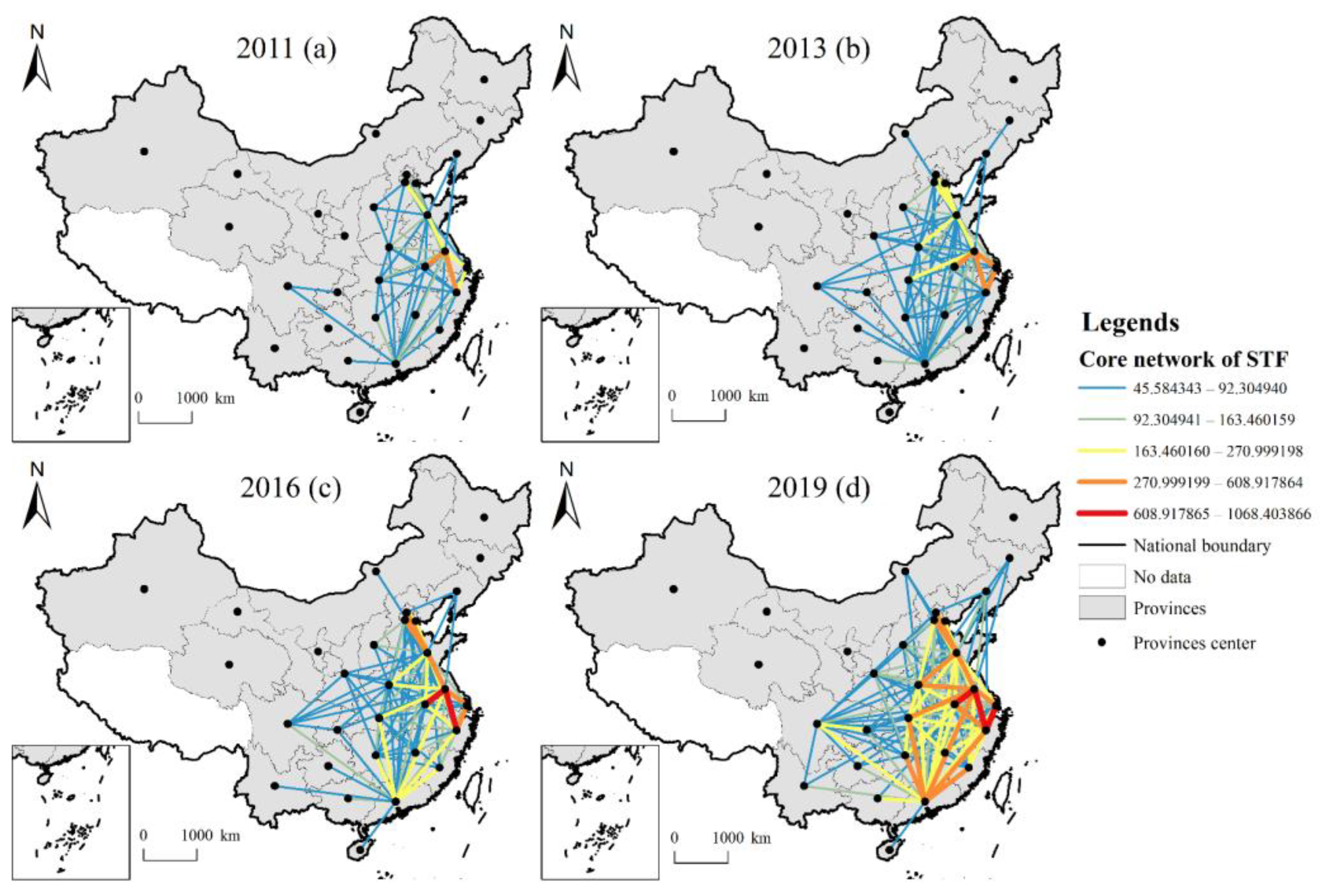
4.1.1. Analysis of the Overall Characteristics of Network Structure

To better reflect the changing trend and dynamic evolution process of the spatial structure of STFN, this article relies on the ArcGIS 10.7 visualisation platform and selects four time points, 2011, 2013, 2016, and 2019, to visualise the structure of STFN, as shown in Figure 2.

In 2011, the structure of the STFN was not yet obvious, and the core network was weak overall. The network linkages were mainly reflected in the BTH region with Beijing as the core, and the YRD region with Jiangsu and Zhejiang as the core. The BTH and the YRD, as important national centres of economic development, were firstly emerged as core network centres, and the strength of the network linkages reached the second level (the grading is shown in different colours in the chart, from red to blue for levels 1 to 5, respectively). The central and western parts of the country only showed sparse network relationships, and the strength of the association of the STFN across the country at this time had yet to be strengthened.

In 2013, the radiation effect of the core network of the STFN expanded, and the network connection of various regions increased. The centre of the YRD network with Shanghai as the core gradually emerged, and for the first time, a third-tier network connection emerged between Henan and the BTH, and Hubei and the YRD, with the network radiation gradually shifting to the central part of the country. As an important national transport hub centre, Hubei plays the role of linking the east with the west, thus establishing a spatial structure layout of the core network that runs East–West. At the same time, as urban financial resources spread and gathered, the links between Sichuan and Guangdong and other core network regions were gradually strengthened, the connectivity of the STFN gradually increased, and the network structure was gradually clarified.

In 2016, the strength of the STFN linkage in the PRD region, with Guangdong as the core, reached the third level. And the network linkage had gradually radiated to the Guangdong region, with the first level of network linkage appearing in the YRD region for the first time. The triangular network structure consisting of the BTH–YRD–PRD gradually became the core structure of the STFN, and the cross-regional network structure linkages gradually strengthened.

In 2019, the cross-regional network structure was more closely linked as the spread of STF resources across the regions expanded and economic exchanges strengthened. The strength of the network structure linkages in the YRD region, with Guangdong as its core, had reached the second level. The triangular network consisting of the BTH–YRD–PRD was gradually becoming more firmly established in the overall network structure, and the network structure was becoming more stable. It can be found that the structure of the STFN had a high similarity with other financial network structures, and showed a similar trend of spatial evolution [41].

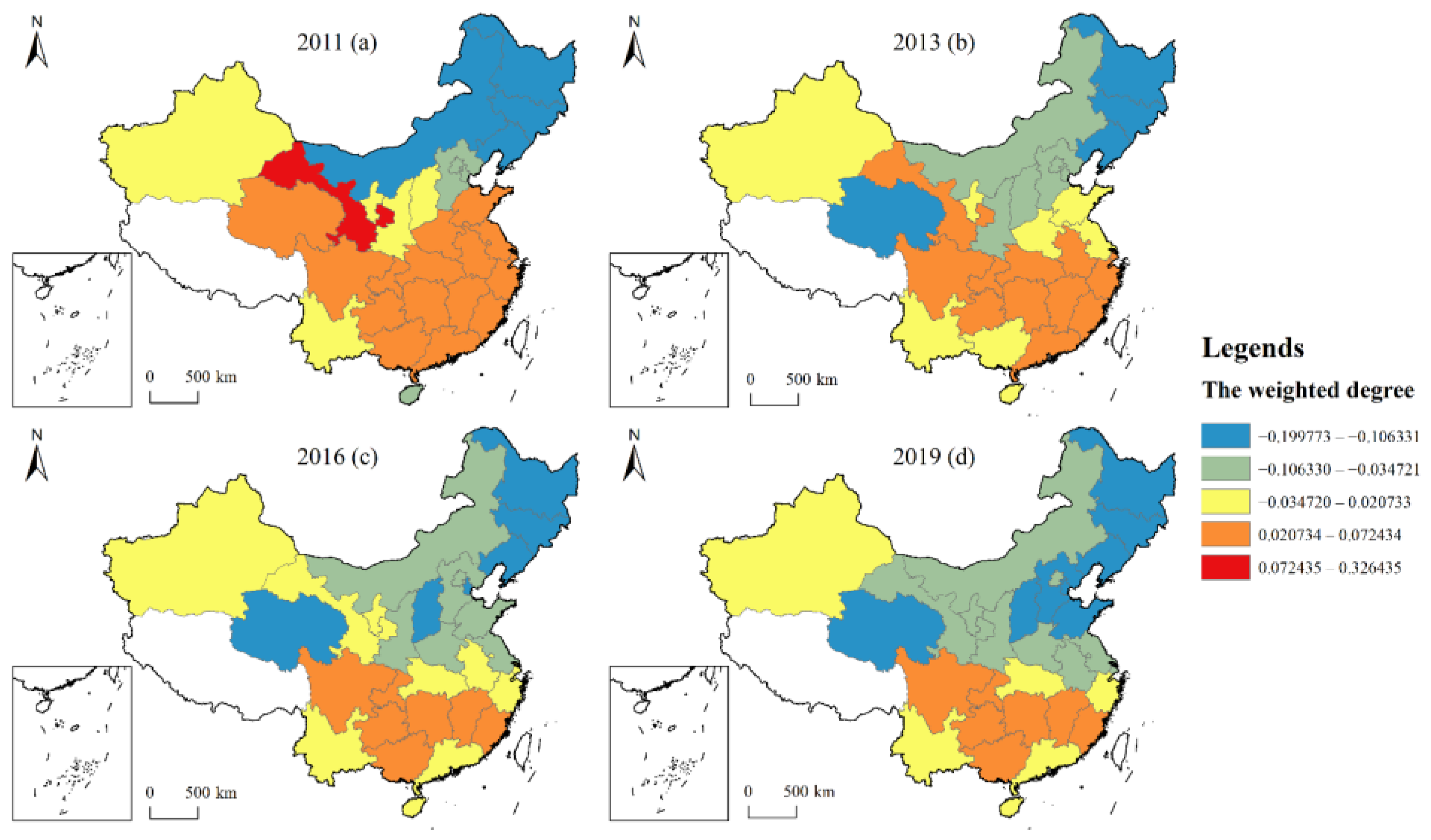
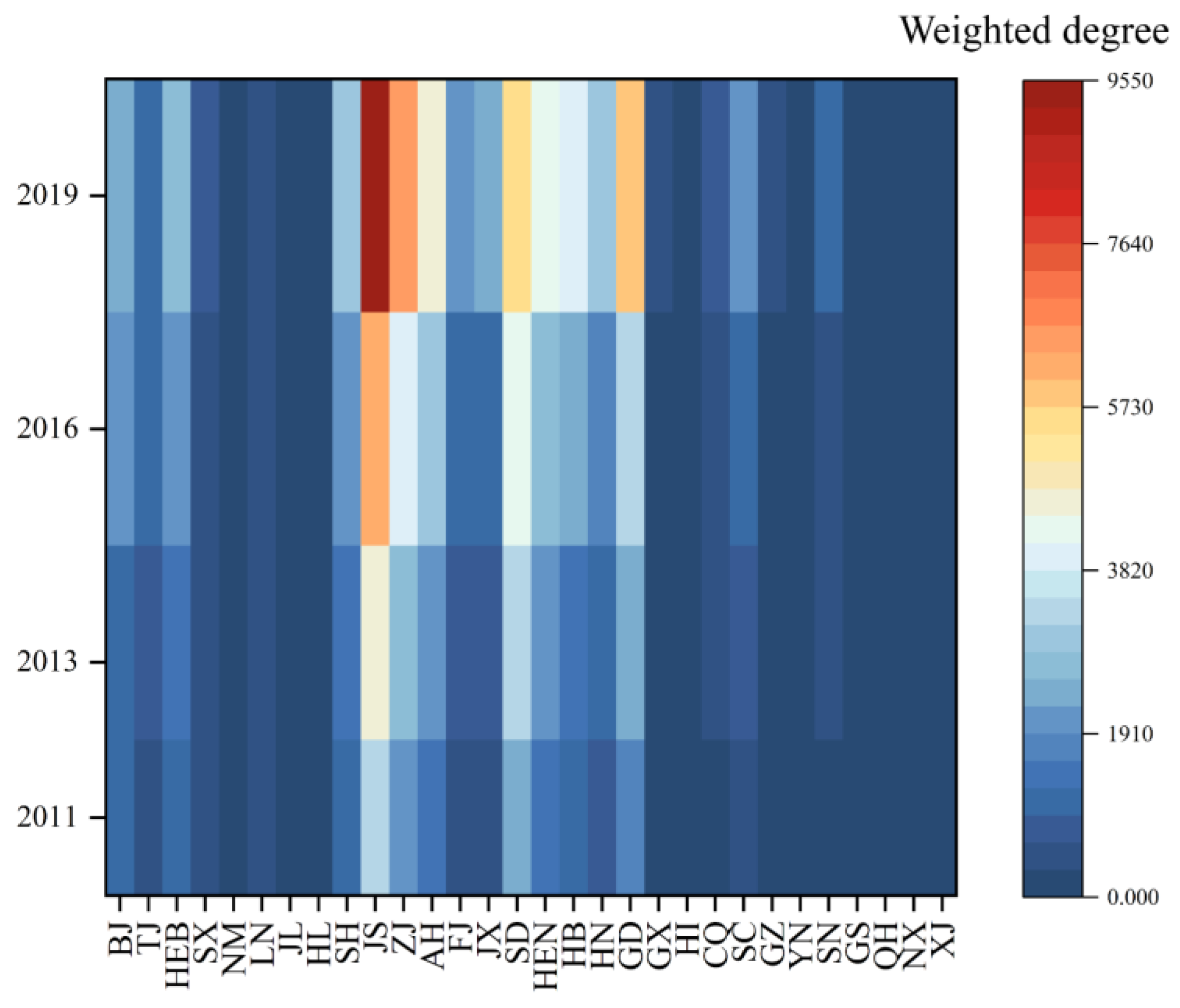
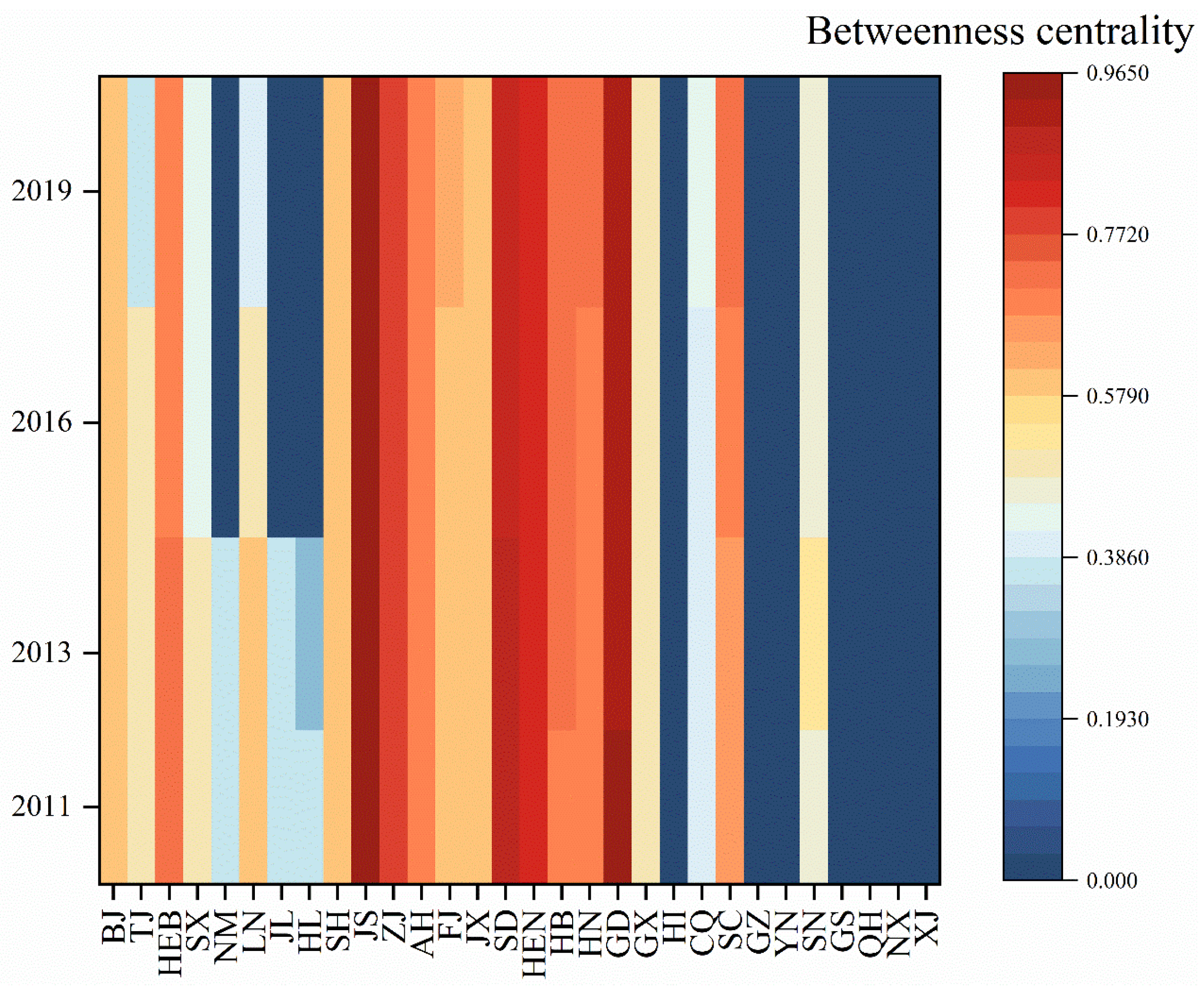
4.1.2. Evolutionary Analysis of Network Node Characteristics

The spatial and temporal evolution of the weighted degree value of the STFN from 2011 to 2019 is shown in Figure 3 (because the core network screened out regions with lower network correlation than the average, the weighted degree value of the network in some regions was zero during the study period). On the whole, the weighted degree value of the study area gradually increased and the network association gradually strengthened during the whole study period. Among them, Jiangsu, Zhejiang, Shandong, and Guangdong have always been in the forefront and in the first echelon, occupying a core position in the spatial network correlation of STF, with strong radiation ability. The above regions are located in the eastern coastal areas of China, with superior geographical locations and rich scientific and technological financial resources. Anhui, Henan, and Hubei regions are in the second tier and have a strong driving force for the development of STF. These regions are located in the central region and play an important role in connecting the east and west and running through the north and south, and have gradually become an important hub for the development of STF in China.

The spatio-temporal evolution of the betweenness centrality of STFN from 2011 to 2019 is shown in Figure 4. On the whole, the betweenness centrality of Jiangsu, Shandong, Guangdong, Henan, and Zhejiang is always in the first echelon, showing strong control over other provinces. Hebei, Anhui, Hunan, Hubei, and Sichuan are in the second tier, while Beijing, Shanghai, Fujian, and Jiangxi are in the third tier. During the study period, the overall fluctuation of the betweenness centrality of the above regions was small, and the echelon structure did not change significantly, indicating that the central and eastern coastal areas had high mediating ability and played a strong role in resource allocation and control. Some northern provinces, such as Inner Mongolia, Shanxi, and northeast China, show a declining trend of betweenness centrality, indicating that their ability to control the correlation between other provinces is weakened, and they are in the edge position and controlled position of the network.

4.2. Analysis of the Impact Effect of Science and Technology Finance Networks on Carbon Emissions

4.2.1. Benchmark Regression

Table 3. Descriptive statistics.

Variable	Obs.	Mean	Std. Dev.	Min.	Max.
Carbon emissions	270	42,772.995	30,037.198	4885.542	150,828.459
Weighted degree value	270	1329.234	1628.447	0.000	9545.792
Betweenness centrality	270	12.452	21.426	0.000	83.020
Residents’ affluence	270	30,408.495	10,204.927	14,988.680	73,848.500
Energy consumption	270	1950.275	1386.072	185.280	6696.000
Industrial structure	270	46.384	9.682	29.700	83.500
Environmental pollution	270	0.521	0.533	0.000	2.585

shows the descriptive statistics of relevant variables, and

Table 4. Benchmark regression results.

	(1) Y(ln)	(2) Y(ln)	(3) Y(ln)
Degree(ln)	−0.0513	−0.1129 ***	−0.1071 ***
	(0.0312)	(0.0302)	(0.0294)
Betweenness(ln)	0.0207 ***	0.0128 **	0.0117 **
	(0.00567)	(0.0050)	(0.0048)
RA(ln)		−0.3477 **	−0.0997
		(0.1676)	(0.0788)
EC(ln)		0.6241 ***	0.6542 ***
		(0.0874)	(0.0786)
IS(ln)		−0.1796 **	−0.1177
		(0.0886)	(0.0776)
EP(ln)		0.0214 **	0.0215 **
		(0.0108)	(0.0104)
cons	10.72 ***	10.7912 ***	7.8472 ***
	(0.183)	(1.7970)	(0.3912)
Time fixed effects	YES	YES	NO
Provincial fixed effects	YES	YES	YES
N	233	227	227
adj. R2	0.009	0.274	0.287

Note: Standard errors in parentheses, ** p < 0.05, *** p < 0.01.

reports the regression results for the impact of STFN on CE. Model (1) is the result of the influence of the weighted degree value and betweenness centrality on CE under the double fixed effect. The coefficient of the weighted degree value is negative, but it is not statistically significant, indicating that it may have a certain negative effect on CE. The coefficient of the betweenness centrality is positive and passes the significance level of 1%, indicating that the betweenness centrality has a strong positive effect on carbon emissions. Model (2) and model (3) represent the regression results for double fixed effects and single fixed effects after adding control variables, respectively. All the variables passed the significance test, so we believe that there is a significant missing variable problem in the separate regression between the core explanatory variable and the explained variable. Both model (2) and model (3) show that the weighted degree value of the STFN shows a significant negative effect on CE at the 1% level, indicating that the more a province is at the centre of the network, the stronger the strength of its ties with other regions; the stronger its overall control in the network, the stronger its ability to gather financial resources and science and technology; the higher its level of science and technology, the more diverse its financing modes and the higher its efficiency in using resources, which is conducive to reducing CE, and hypothesis 1 has been verified. Simultaneously, both model (2) and model (3) show that the betweenness centrality of the STFN shows a more significant positive effect on CE at the 5% level, with provinces in intermediary locations, indirectly establishing links with other provinces, accelerating the creation of new economic models while resources such as STF are widely disseminated. The convenience of access to capital causes residential consumers to increase consumption, and the convenient financing conditions cause corporate producers to increase the amount of production inputs and expand their business activities. The wealth effect and scale effect caused by the increase in consumption and production are less than the technology effect caused by the absorption of technological resources, which leads to an increase in CE, and hypothesis 2 has been verified.

From the control variables, the coefficient of urban residents’ affluence level is negative and significant at the 5% significance level, which may be due to the fact that as residents’ income level increases, their awareness of “green consumption” gradually increases and they are willing to choose low-carbon and environmentally friendly products or services to reduce their negative impact on the environment. The coefficient of energy consumption is positive and significant at the 1% significance level, indicating that electricity consumption is the main factor affecting CE in each region, and thermal power generation is still the main mode of power generation. The regression coefficient of the industrial structure is negative and significant at the 5% significance level, indicating that the tertiary sector in each region can effectively play its role in energy saving and emission reduction, thus contributing to the reduction of CE. The regression coefficient of environmental pollution is positive and significant at the 5% significance level, indicating that industrial environmental pollution can significantly enhance CE, which is in line with reality.

4.2.2. Robustness Tests

To further test the impact of the STFN on CE, this study conducted robustness tests by replacing the explained variables and core explanatory variables.

Firstly, the explained variables were replaced by data on CE from the eight main fossil energy consumptions with the CE indicator from Carbon Emission Accounts and Datasets (CEADs).

Table 5. Robustness test results.

	(1)	(2)	(3)	(4)
	Y(ln)	Y(ln)	Y(ln)	Y(ln)
Degree(ln)	−0.0203	−0.0794 ***	−0.0554	−0.2075 ***
	(0.0293)	(0.0303)	(0.0391)	(0.0369)
Betweenness(ln)	0.0175 ***	0.0118 **
	(0.00533)	(0.0050)
Closeness(ln)			0.0232 **	0.0451 ***
			(0.0112)	(0.0093)
RA(ln)		0.2478		−0.3028 *
		(0.1682)		(0.1609)
EC(ln)		0.4698 ***		0.7596 ***
		(0.0877)		(0.0832)
IS(ln)		−0.0886		−0.1952 **
		(0.0889)		(0.0850)
EP(ln)		0.0246 **		0.0238 **
		(0.0108)		(0.0103)
cons	5.679 ***	0.5973	10.75 ***	9.8922 ***
	(0.172)	(1.8035)	(0.215)	(1.7150)
Time fixed effects	YES	YES	YES	YES
Provincial fixed effects	YES	YES	YES	YES
N	233	227	233	227
adj. R2	0.135	0.278	−0.035	0.333

Note: Standard errors in parentheses, * p < 0.1, ** p < 0.05, *** p < 0.01.

(1)–(2) shows the regression results after replacing the variables. Although there are slight differences in the values of the regression coefficients from the previous findings, the influence relationship between the dependent and independent variables remains unchanged, and the weighted degree values and betweenness centrality are significant at 1% and 5% significance levels, respectively, after the addition of control variables, which largely remain consistent with the benchmark results in Table 3, demonstrating the robustness of the results.

Secondly, by replacing the core explanatory variables and replacing betweenness centrality with closeness centrality, both closeness centrality and betweenness centrality are indicators of network structure and are used to characterise the importance of nodes in the network. Table 5(3)–(4) presents the regression results after replacing the variables, which are generally consistent with the previous results, and model (4) is significant at the 1% significance level, indicating that the closeness centrality of the STFN also has a significant positive effect on CE, proving the results to be robust.

From the regression results of robustness, the regression coefficients after replacing both the explained variables and the core explanatory variables are significant, which is consistent with the previous results, and the previous reference estimated coefficients are significant under both single and double fixed effects. Accordingly, the benchmark regression model constructed in this article is considered to be strongly robust, with the weighted degree value of the STFN having a significant inhibitory effect on CE and the betweenness centrality having a promoting effect on CE.

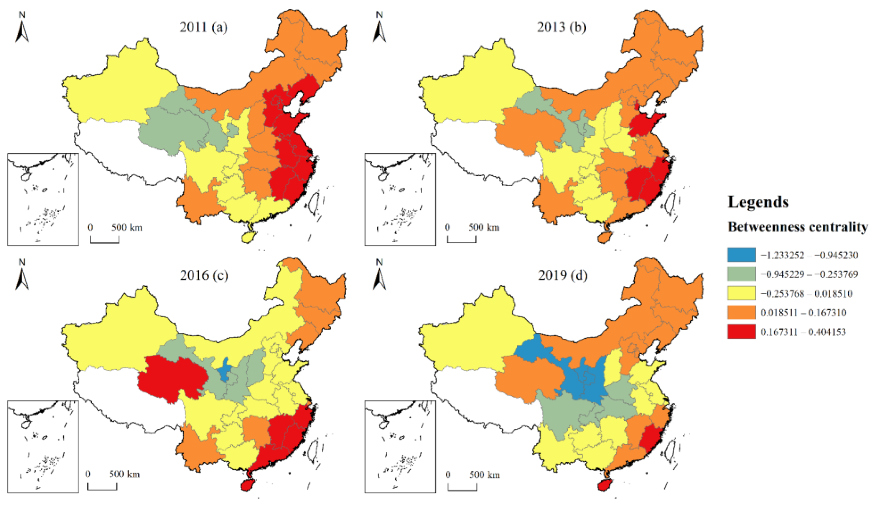
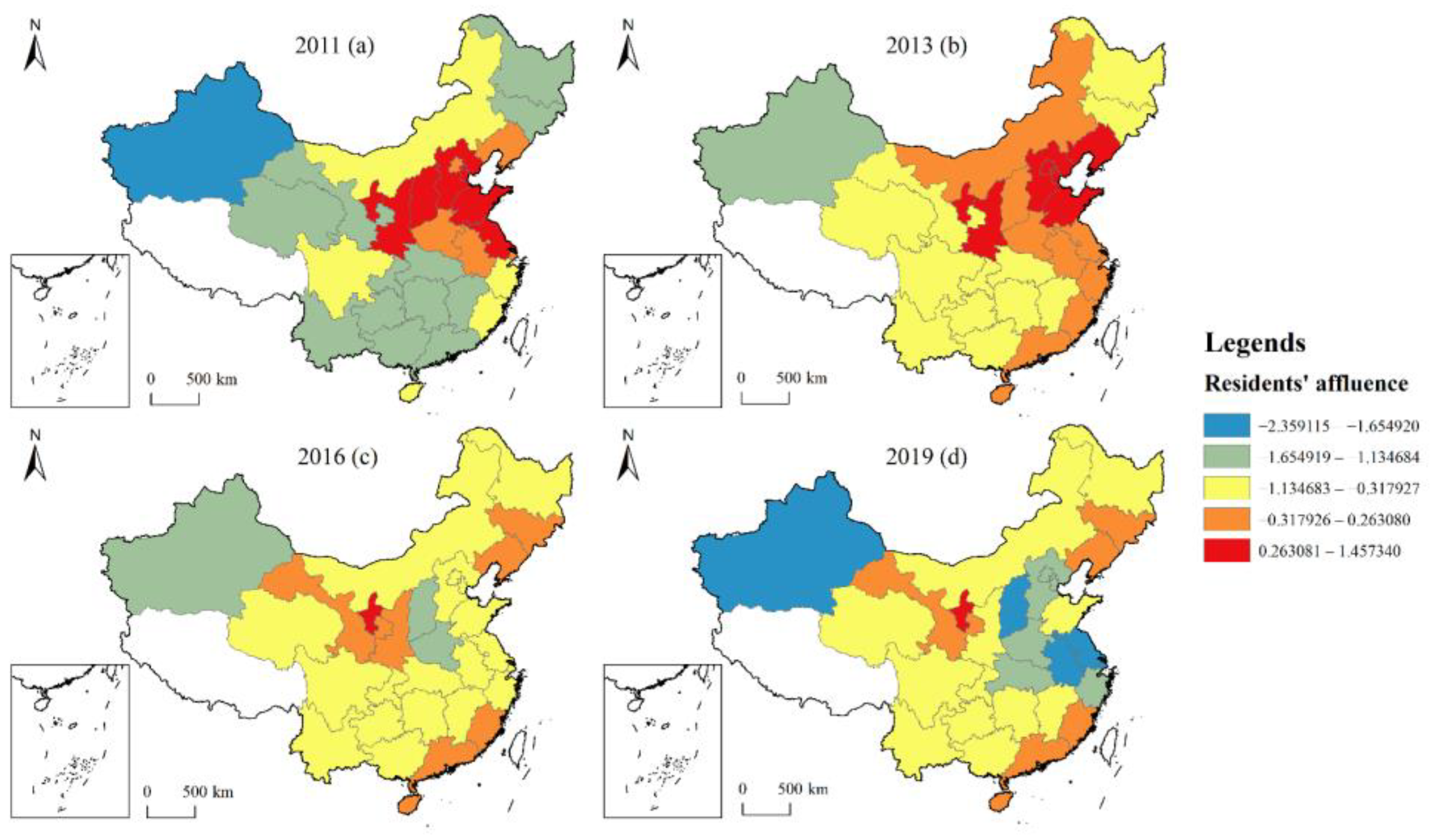
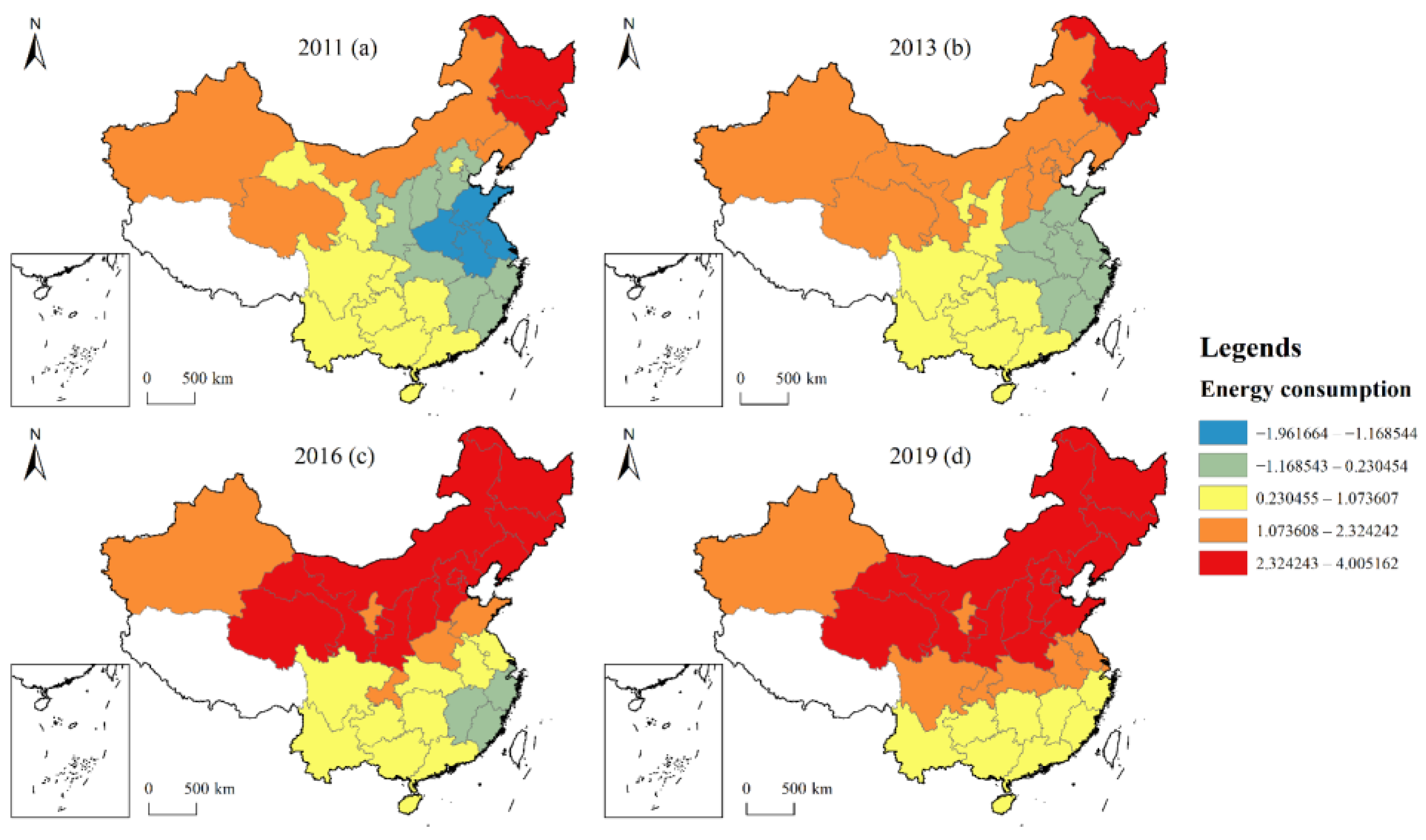
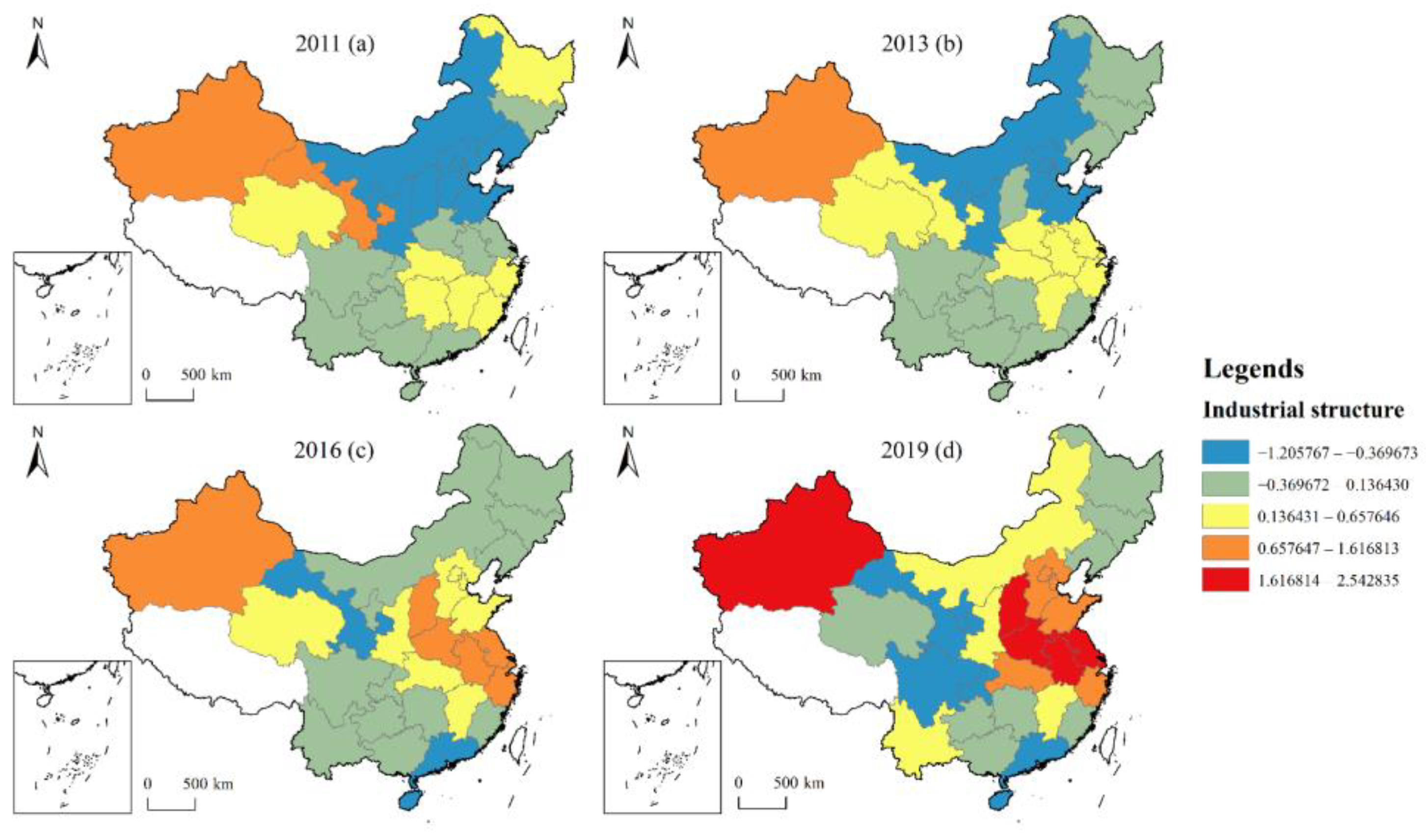
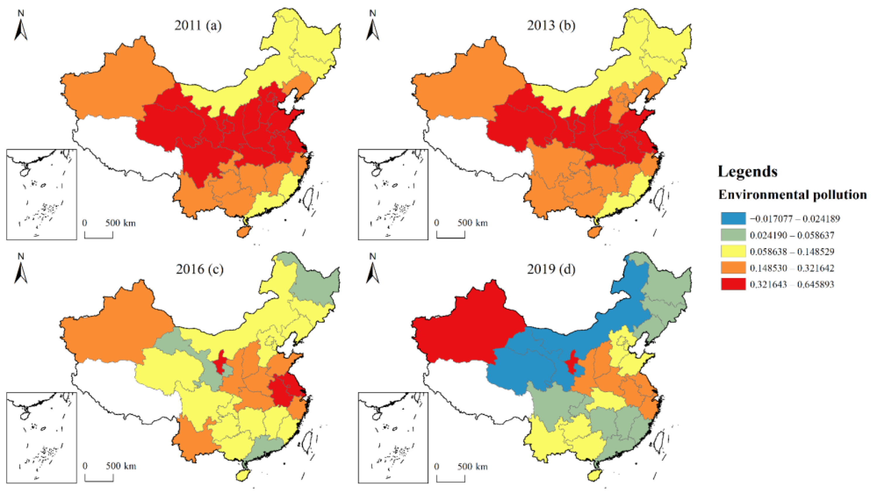
4.3. Analysis of the Spatial and Temporal Heterogeneity of the Influencing Factors

The GTWR model incorporates the spatio-temporal characteristics of the data into the regression model, allowing for better observation of the spatio-temporal evolutionary characteristics of the data and influence relationships [42]. As can be seen from the previous benchmark regression results, both the core explanatory and control variables selected for this article have significant effects on CE; at the same time, the existing research holds that the impact of GDP and the industrial structure, etc., on CE shows evidence of spatial heterogeneity [43].

Accordingly, the following section constructs the GTWR model based on panel data of 30 Chinese provinces from 2011 to 2019, calculates and analyses the relationship of the six variables (the weighted degree value, betweenness centrality of STFN, residents’ affluence, energy consumption, industrial structure, and environmental pollution) on CE in each region, and the spatial distribution of the influencing factors was plotted by the natural breakpoint method. Based on the analysis of the results, it is clear that the regression coefficients of the influencing factors of CE show a significant pattern of spatial and temporal divergence.

Table 6. Parameters of GTWR.

Model Parameters	Bandwidth	AICc	R2	Adjusted R2
Value	0.114996	5530.39	0.977392	0.976876

shows the estimated result of the GTWR. R2 and Adjusted R2 can be used to illustrate the fitting degree of the model, and their values are both higher than 0.9, indicating that the GTWR model can effectively measure the spatio-temporal heterogeneity and the degree of influencing factors.

In terms of the spatial distribution of the impact of the weighted degree value on CE (see Figure 5), in general, the influence coefficient of the weighted degree value of the STFN is mainly negative in space. The positive value of the weighted coefficient is mainly concentrated in the south, indicating that the economic and wealth effects brought about by the strengthening of STF links in the south are greater than the technological effects brought about by the development of science and technology, thus showing a significant positive impact on CE. The high negative value of the weighted coefficient is mainly concentrated in the northeast and the BTH regions, probably because the supply-side reform has had a greater impact on the economic development of these regions in recent years, and the policy of “removing production capacity” has forced traditional industries to transform and develop. As these regions become more strongly connected to other regions in the network, they will drive technological progress and promote the transformation of industrial energy structures, thereby reducing CE. Over time, the positive value of the weighted impact coefficient gradually decreases between 2011 and 2019, and the negative value of the impact coefficient gradually spreads from the north to the south, suggesting that the strengthening of technological and financial connections and economic exchanges between regions will gradually curb CE.

In terms of the spatial distribution characteristics of the impact of the betweenness centrality on CE (see Figure 6), from 2011 to 2019, the positive high values of the betweenness centrality influence coefficient are mainly concentrated in the eastern coastal region, and the positive impact is gradually decreasing. The negative value of the influence coefficient is gradually increasing, and the negative values are mainly distributed in the northwest, southwest, and central China. For the eastern coastal regions, the weighted degree value of the STFN is higher and they are at the centre of the network. These regions have already developed to a certain level of science and technology and economic level, so when financial capital and technology resources are disseminated and flow spatially, the technology gain brought is not enough to form a new technology breakthrough force to improve the existing energy consumption structure, but the increase in the betweenness centrality will stimulate consumption and increase the demand for energy, thus increasing CE. On the contrary, for regions geographically located in central and western China, the northwest region, with its abundant solar and wind power resources, has gathered a large number of wind and solar power projects, while the western region is also an important ecological function area, placing more prominence on resource conservation and environmental protection, actively developing new energy equipment, comprehensive resource utilisation, and other industries, with increasing coordination between industrial development and resources and the environment. The development of the network’s intermediary capacity is more prominent, and it is more effective in absorbing and transforming scientific and technological resources, thus demonstrating a suppressive effect on CE.

In terms of the spatial distribution characteristics of the impact of residents’ affluence on CE (see Figure 7), in general, the negative effect of residents’ affluence on CE is greater, with the positive high value of the influence coefficient of residents’ affluence mainly distributed in northern China from 2011 to 2013, and gradually changing to negative values from 2016 to 2019. This indicates that the region has increased its consumption expenditure in daily life as its income level rises, which has contributed to the consumption of energy and other resources. The negative high-value areas show a spatial pattern of decreasing and then increasing, concentrated in Xinjiang, Shanghai, Jiangsu, and Anhui, etc. The reason for this is that the higher the per capita income of residents in these regions, the stronger people’s awareness of “green and low-carbon”, and the more willing they are to consume green and environmentally friendly products, forcing enterprises to make a green transformation, thus reducing CO₂ emissions; this conclusion is confirmed in the study of the effect of different household income levels on CE [44]. The regions with lower absolute values of the influence coefficient of residents’ affluence gradually stabilised from 2016 to 2019, mainly in the northeast, northwest, and southeast coastal regions, where the influence of residents’ per capita income on CE is weaker.

In terms of the spatial distribution characteristics of the impact of energy consumption on CE (see Figure 8), the influence coefficient of energy consumption mainly shows a strong positive impact, and the influence is becoming more and more significant. Some studies believe that energy intensity has the greatest impact on CE, and the reduction in energy intensity can effectively promote CE reduction, which is consistent with the conclusion of this study [45]. The positive high-value area was mainly concentrated in the northeast from 2011 to 2013, and the distribution of the positive high-value area gradually spread to north and northwest China from 2016 to 2019, while the negative influence area gradually decreased until it disappeared from 2011 to 2019. Although China is working on new energy generation to improve the environment, thermal power generation is still dominant. According to statistics, thermal power generation accounts for about 70% of the country’s total electricity generation, and most thermal power plants generate thermal power by burning coal, which has a high proportion of carbon content, and thermal power generation is the main driver of increased CE, so these regions will have a significant contribution to CE.

In terms of the spatial distribution of the impact of industrial structure on CE (see Figure 9), the influence coefficient is mainly negative and fluctuates from 2011 to 2019. Some studies have found that industrial structure has different impacts on regional CE, and industry and construction industry have significant positive impacts on CE, which is consistent with the conclusion of this paper that the tertiary industry reduces CE to a significant extent [46]. The areas with high negative values of industrial structure impact coefficients gradually shift from north China to the northwest and the southwest. The spatial pattern of positive high-value regions is more stable, mainly in Xinjiang and east China. Different industries have different energy consumption elasticities, with Xinjiang and east China having a more stable industrial structure, and regions with a lower share of tertiary industries relying more on traditional energy consumption than those with a higher share. Southwest China, such as Sichuan, has a significant negative impact coefficient on industrial structure, indicating that the region has a higher share of tertiary industries, which brings into play the energy-saving and emission-reducing capacity of the tertiary sector and therefore has a stronger inhibiting effect on CE. The impact coefficient for Shanxi is also significantly negative. Shanxi, as China’s major coal production province, has a predominantly coal-based energy consumption, suggesting that the active development of Shanxi’s tertiary sector will significantly reduce its reliance on energy sources such as coal, showing a significant positive spillover effect and thus reducing CE.

In terms of the spatial distribution characteristics of the impact of environmental pollution on CE (see Figure 10), in general, the influence coefficient of environmental pollution on CE mainly shows a positive effect; this effect has also been confirmed in the relevant literature [47]. However, with the passage of time, the positive high-value coefficient gradually decreases until the negative value of the impact coefficient appears in 2019, and the negative high value is mainly concentrated in Inner Mongolia, Shaanxi, and Qinghai regions. It indicates that with the improvement of science and technology, the innovation ability of industrial energy technology has increased, promoting the transformation of energy structure and reducing the emission of waste gas pollutants. The optimisation of industrial structure and energy structure, complete new energy devices and equipment, and the promulgation of ecological and environmental protection policies have enabled the regions to fully absorb the green effects brought about by the optimisation of industrial structure and technological upgrading, significantly reducing the pollution emissions brought about by industrial development in each region, and thus curbing the increase in CE.

5. Conclusions and Policy Implications

With the active promotion of the “carbon peaking and carbon neutrality” goals, the gradual improvement and maturity of the urban financial network system, and the improvement of the technological level of enterprises, it is important to study the impact of the STFN on CE to promote low-carbon development. Based on provincial panel data from 2011 to 2019 in China, this article uses the level of development of STF in each province as an indicator to construct a STFN, and selects the weighted degree value and betweenness centrality as typical network structure indicators to explore their impact on CE. The following conclusions are drawn:

(1) From 2011 to 2019, the spatial structure of China’s STFN changed significantly. From 2011 to 2016, the BTH and the YRD regions were mainly used as network centres, and with the strengthening of STF connections in various regions, the network centres expanded their radiation range, and the network structure of the PRD region with Guangdong as the core began to emerge. By 2019, the triangular structure consisting of BTH–YRD–PRD was becoming firmly established in the overall network and the network structure was stabilising.

(2) The results of the benchmark regression show that the weighted degree value of the STFN has a significant inhibiting effect on CE, indicating that the higher the weighted degree value of the region’s ability to control financial, technological, and other resources can effectively promote the region’s economic transformation and optimal development, thereby reducing CE. Betweenness centrality, on the other hand, has a positive effect on CE, indicating that the higher the betweenness centrality, the higher the absorption and transformation of resources, the higher the consumption and production, which will increase CE by expanding production and increasing the demand for energy. The robustness results also show that the model is robust by replacing the explained and core explanatory variables.

(3) In exploring the study of the spatio-temporal heterogeneity of the STFN on CE, it is found that the weighted degree value has a more significant CE reduction effect on the eastern region with a higher level of economic development and technology, while the betweenness centrality has a more significant CE reduction effect on the central and western regions, but shows a significant promotion effect on CE in the eastern region.

(4) There is significant spatio-temporal heterogeneity in the effects of residents’ affluence, energy consumption, industrial structure, and environmental pollution on CE. From 2011 to 2019, the influence of residents’ affluence and industrial structure on CE mainly showed negative effects, with the negative influence of residents’ affluence gradually increasing, while the negative influence of the industrial structure is gradually weakening. The positive effect of energy consumption gradually strengthened, and the effect of environmental pollution gradually changed from positive to negative from 2011 to 2019.

Based on the above findings, this article makes the following policy recommendations:

(1) Different network locations represent different advantages for each region in terms of access to information, technology, and capital. Regions located at the centre of the network should strengthen their control in the overall network, give full play to their geographical advantages of financial resources concentration, high level of science and technology, and abundant human resources, actively promote the transformation and development of the energy structure, and break through the bottleneck of industrial structure consolidation, and thus improve the ability to reduce CE.

(2) To improve the role of carbon reduction in areas with high betweenness centrality, while playing the role of the intermediary position, the absorption and transformation of STF resources should be emphasised. Strengthen financial connections with network central provinces and fringe cities, absorb technology and capital from network central provinces, and at the same time channel resources to network fringe provinces, thus strengthening the STF ties between regions and solidifying the structure of the STFN, which in turn will promote and enhance the CE suppression role of neighbouring provinces through positive spillover effects.

(3) Focus on the imbalance of regional development in the STFN according to local conditions. While continuing to strengthen the CE reduction effect in the central provinces of the eastern network, financial ties between the east and the more economically underdeveloped regions of the central and western regions should also be strengthened. Local fiscal policies should be used to encourage the relocation of eastern science and technology enterprises to the central and western parts of the country, to drive the flow and diffusion of capital, talent, and technology to the central and western parts of the country, to actively explore new financing models, and to provide financial reserves and technical support for creating a favourable innovation environment.

Even though this study provides a certain complement to the lack of CE-related studies from a micro perspective and provides a reference for the study of the CE reduction effect of STF, the shortcomings of this study need further improvement. Due to the availability of data, there are still certain deficiencies in the measurement of STF, and CE data of only 30 Chinese provinces from 2011–2019 were selected. Further studies could be more in-depth in terms of data richness and the specific mechanistic effects of the STFN on CE, as well as how complex networks analysis can be used in empirical studies of econometric factors.

References

1. Dale, S. BP Statistical Review of World Energy; BP Plc: London, UK, 2021; pp. 14–16. [Google Scholar]
2. Wen, Y.; Hu, P.; Li, J.; Liu, Q.; Shi, L.; Ewing, J.; Ma, Z. Does China’s carbon emissions trading scheme really work? A case study of the hubei pilot. J. Clean. Prod. 2020, 277, 124151. [Google Scholar] [CrossRef]
3. Xu, X.; Zhao, T.; Liu, N.; Kang, J. Changes of energy-related GHG emissions in China: An empirical analysis from sectoral perspective. Appl. Energy 2014, 132, 298–307. [Google Scholar] [CrossRef]
4. Pan, B.; Zhang, Y. Impact of affluence, nuclear and alternative energy on US carbon emissions from 1960 to 2014. Energy Strat. Rev. 2020, 32, 100581. [Google Scholar] [CrossRef]
5. Shahbaz, M.; Nasir, M.A.; Roubaud, D. Environmental degradation in France: The effects of FDI, financial development, and energy innovations. Energy Econ. 2018, 74, 843–857. [Google Scholar] [CrossRef]
6. Huang, L.; Zhao, X. Impact of financial development on trade-embodied carbon dioxide emissions: Evidence from 30 provinces in China. J. Clean. Prod. 2018, 198, 721–736. [Google Scholar] [CrossRef]
7. Tong, Y.; Jin, L.; Zhang, Y. Research on the carbon emission reduction effect of science and technology finance: An analysis of quasi-natural experiments based on the pilot project of “Promoting the integration of science, technology and finance”. J. Southwest Univ. Nat. Sci. Ed. 2023, 45, 175–187. (In Chinese) [Google Scholar]
8. Strumsky, D.; Thill, J.C. Profiling US metropolitan regions by their social research networks and regional economic performance. J. Reg. Sci. 2013, 53, 813–833. [Google Scholar] [CrossRef]
9. Sigler, T.J.; Martinus, K. Extending beyond ‘world cities’ in World City Network (WCN) research: Urban positionality and economic linkages through the Australia-based corporate network. Env. Plan. A 2017, 49, 2916–2937. [Google Scholar] [CrossRef]
10. Kleindorfer, P.R.; Wind, Y.J.R.; Gunther, R.E. The Network Challenge: Strategy, Profit, and Risk in an Interlinked World, 1st ed.; Prentice Hall Professional: Upper Saddle River, NJ, USA, 2009; pp. 1–20. [Google Scholar]
11. Yu, L.; Li, W.; Chen, Z.; Shi, M.; Liu, H. Multi-stage collaborative efficiency measurement of sci-tech finance: Network-DEA analysis and spatial impact research. Econ. Res.-Ekon. Istraživanja 2022, 35, 300–324. [Google Scholar] [CrossRef]
12. Lu, Y.; Guo, J.; Ahmad, M.; Zhang, H. Can Sci-Tech Finance Pilot Policies Reduce Carbon Emissions? Evidence from 252 Cities in China. Front. Environ. Sci. 2022, 10, 933162. [Google Scholar] [CrossRef]
13. Li, L.; Mao, D. The mechanism of government credit to promote science and technology innovation and financial innovation—A study based on the practice of science and technology finance network in Suzhou. Econ. Syst. Reform 2012, 4, 52–56. (In Chinese) [Google Scholar]
14. Xu, Y.; Yu, L. A simulation study on the evolution of regional science and technology financial network based on CAS. Sci. Technol. Manag. Res. 2020, 40, 46–56. (In Chinese) [Google Scholar]
15. Tao, M.; Huang, Y.; Tao, H. Urban network externalities, agglomeration economies and urban economic growth. Cities 2020, 107, 102882. [Google Scholar]
16. Feng, Z.; Cai, H.; Chen, Z.; Zhou, W. Influence of an interurban innovation network on the innovation capacity of China: A multiplex network perspective. Technol. Forecast. Soc. Chang. 2022, 180, 121651. [Google Scholar] [CrossRef]
17. Mai, B.; Liu, J.; Sandra, G. Network effects in the academic market: Mechanisms for hiring and placing PhDs in communication (2007–2014). J. Commun. 2015, 65, 558–583. [Google Scholar] [CrossRef]
18. Borgatti, S.P. Centrality and network flow. Soc. Netw. 2005, 27, 55–71. [Google Scholar] [CrossRef]
19. Teece, D. Firm organization, industrial structure, and technological innovation. J. Econ. Behav. Organ. 1996, 31, 193–224. [Google Scholar] [CrossRef]
20. Liu, M.; Li, H.; Li, C. Digital transformation, financing constraints and enterprise performance. Eur. J. Innov. Manag. 2023. [Google Scholar] [CrossRef]
21. Guan, J.; Zuo, K.; Chen, K.; Yam, R.C. Does country-level R&D efficiency benefit from the collaboration network structure? Res. Policy 2016, 45, 770–784. [Google Scholar]
22. Ozmel, U.; Reuer, J.J.; Gulati, R. Signals across multiple networks: How venture capital and alliance networks affect interorganizational collaboration. Acad. Manag. J. 2013, 56, 852–866. [Google Scholar] [CrossRef]
23. Tang, E.; Peng, C.; Xu, Y. Changes of energy consumption with economic development when an economy becomes more productive. J. Clean. Prod. 2018, 196, 788–795. [Google Scholar] [CrossRef]
24. Wang, S.; Liu, J.; Qin, X. Financing constraints, carbon emissions and high-quality urban development—Empirical evidence from 290 Cities in China. Int. J. Environ. Res. Public Health 2022, 19, 2386. [Google Scholar] [CrossRef] [PubMed]
25. Chen, X.; Chen, Z. Can green finance development reduce carbon emissions? Empirical evidence from 30 Chinese provinces. Sustainability 2021, 13, 12137. [Google Scholar] [CrossRef]
26. Miao, C.; Duan, M.; Zuo, Y.; Wu, X. Spatial heterogeneity and evolution trend of regional green innovation efficiency--an empirical study based on panel data of industrial enterprises in China’s provinces. Energy Policy 2021, 156, 112370. [Google Scholar] [CrossRef]
27. Leiponen, A.; Drejer, I. What exactly are technological regimes? Intra-industry heterogeneity in the organization of innovation activities. Res. Policy 2007, 36, 1221–1238. [Google Scholar] [CrossRef]
28. Sun, J.; Guo, X.; Wang, Y.; Shi, J.; Zhou, Y.; Shen, B. Nexus among energy consumption structure, energy intensity, population density, urbanization, and carbon intensity: A heterogeneous panel evidence considering differences in electrification rates. Env. Sci Pollut. Res. 2022, 29, 19224–19243. [Google Scholar] [CrossRef] [PubMed]
29. Zhu, K.; Gu, Z.; Li, J. Analysis of the China’s Interprovincial Innovation Connection Network Based on Modified Gravity Model. Land 2023, 12, 1091. [Google Scholar] [CrossRef]
30. Li, H.; Shang, Q.; Deng, Y. A modified gravity model based on network efficiency for vital nodes identification in complex networks. arXiv 2022, arXiv:2111.01526. [Google Scholar]
31. Burt, R.S. Models of network structure. Annu. Rev. Sociol. 1980, 6, 79–141. [Google Scholar] [CrossRef]
32. Ding, R.; Ujang, N.; Hamid, H.B.; Manan, M.S.A.; Li, R.; Albadareen, S.S.M.; Nochian, A.; Wu, J. Application of complex networks theory in urban traffic network researches. Netw. Spat. Econ. 2019, 19, 1281–1317. [Google Scholar] [CrossRef]
33. Rey, S.J. Spatial empirics for economic growth and convergence. Geogr. Anal. 2001, 33, 195–214. [Google Scholar] [CrossRef]
34. Fotheringham, A.S.; Crespo, R.; Yao, J. Geographical and temporal weighted regression (GTWR). Geogr. Anal. 2015, 47, 431–452. [Google Scholar] [CrossRef]
35. Chen, Z.; Huang, W.; Zheng, X. The decline in energy intensity: Does financial development matter? Energy Policy 2019, 134, 110945. [Google Scholar] [CrossRef]
36. IPCC. IPCC Guidelines for National Greenhouse Gas Inventories Prepared by the National Greenhouse Gas Inventories Programme; IGES: Tokyo, Japan, 2006. [Google Scholar]
37. Ding, R.; Chen, S.; Zhang, B.; Shen, S.; Zhou, T. The reduce of energy consumption intensity: Does the development of science and technology finance matter? Evidence from China. Energy Rep. 2022, 8, 11206–11220. [Google Scholar] [CrossRef]
38. Cao, H.; You, J.; Lu, R.; Chen, H. An empirical study of China’s technology finance development index. China Manag. Sci. 2011, 19, 134–140. (In Chinese) [Google Scholar]
39. Salahuddin, M.; Alam, K. Internet usage, electricity consumption and economic growth in Australia: A time series evidence. Telemat. Inform. 2015, 32, 862–878. [Google Scholar] [CrossRef]
40. Bhujabal, P.; Sethi, N.; Padhan, P.C. ICT, foreign direct investment and environmental pollution in major Asia Pacific countries. Environ. Sci. Pollut. Res. 2021, 28, 42649–42669. [Google Scholar] [CrossRef] [PubMed]
41. Chen, S.; Ding, R.; Shen, S.; Zhang, B.; Wang, K.; Yin, J. Coordinated development of green finance and green technology innovation in China: From the perspective of network characteristics and prediction. Environ. Sci. Pollut. Res. 2023, 31, 10168–10183. [Google Scholar] [CrossRef] [PubMed]
42. Liu, J.; Zhao, Y.; Yang, Y. A mixed geographically and temporally weighted regression: Exploring spatial-temporal variations from global and local perspectives. Entropy 2017, 19, 53. [Google Scholar] [CrossRef]
43. Li, W.; Dong, F.; Ji, Z. Research on coordination level and influencing factors spatial heterogeneity of China’s urban CO2 emissions. Sustain. Cities Soc. 2021, 75, 103323. [Google Scholar] [CrossRef]
44. Karpinska, L.; Sławomir, Ś. Does a household’s income affect its carbon emissions? Results for single-family homes in Poland. J. Hous. Built Environ. 2023, 11, 1–23. [Google Scholar] [CrossRef]
45. Wang, Z.; Yang, Y. Features and influencing factors of carbon emissions indicators in the perspective of residential consumption: Evidence from Beijing, China. Ecol. Indic. 2016, 61, 634–645. [Google Scholar] [CrossRef]
46. Zheng, H.; Gao, X.; Sun, Q.; Han, X.; Wang, Z. The impact of regional industrial structure differences on carbon emission differences in China: An evolutionary perspective. J. Clean. Prod. 2020, 257, 120506. [Google Scholar] [CrossRef]
47. Chen, L.; Li, H.; Qin, X. Spatial Heterogeneity of Carbon Emissions and Its Influencing Factors in China: Evidence from 286 Prefecture-Level Cities. Int. J. Environ. Res. Public Health 2022, 19, 1226. [Google Scholar] [CrossRef] [PubMed]
Figure 1. Research framework.
Systems 12 00110 g001
Figure 2. Evolution of the spatial pattern of China’s STFN in 2011 (a), 2013 (b), 2016 (c), and 2019 (d).
Systems 12 00110 g002
Figure 3. The weighted degree value of STFN.
Systems 12 00110 g003
Figure 4. The betweenness centrality of STFN.
Systems 12 00110 g004
Figure 5. Spatial evolution of influence coefficient of the weighted degree value in 2011 (a), 2013 (b), 2016 (c), and 2019 (d).
Systems 12 00110 g005
Figure 6. Spatial evolution of influence coefficient of the betweenness centrality in 2011 (a), 2013 (b), 2016 (c), and 2019 (d).
Systems 12 00110 g006
Figure 7. Spatial evolution of influence coefficient of resident affluence in 2011 (a), 2013 (b), 2016 (c), and 2019 (d).
Systems 12 00110 g007
Figure 8. Spatial evolution of influence coefficient of energy consumption in 2011 (a), 2013 (b), 2016 (c), and 2019 (d).
Systems 12 00110 g008
Figure 9. Spatial evolution of influence coefficient of industry structure in 2011 (a), 2013 (b), 2016 (c), and 2019 (d).
Systems 12 00110 g009
Figure 10. Spatial evolution of influence coefficient of environmental pollution in 2011 (a), 2013 (b), 2016 (c), and 2019 (d).
Systems 12 00110 g010