Comparing the Complexity and Efficiency of Composable Modeling Techniques for Multi-Scale and Multi-Domain Complex System Modeling and Simulation Applications: A Probabilistic Analysis

Abstract

Modeling and simulation of complex systems frequently requires capturing probabilistic dynamics across multiple scales and/or multiple domains. Cyber–physical, cyber–social, socio–technical, and cyber–physical–social systems are common examples. Modeling and simulating such systems via a single, all-encompassing model is often infeasible, and thus composable modeling techniques are sought. Co-simulation and closure modeling are two prevalent composable modeling techniques that divide a multi-scale/multi-domain system into sub-systems, use smaller component models to capture each sub-system, and coordinate data transfer between component models. While the two techniques have similar goals, differences in their methods lead to differences in the complexity and computational efficiency of a simulation model built using one technique or the other. This paper presents a probabilistic analysis of the complexity and computational efficiency of these two composable modeling techniques for multi-scale/multi-domain complex system modeling and simulation applications. The aim is twofold: to promote awareness of these two composable modeling approaches and to facilitate complex system model design by identifying circumstances that are amenable to either approach.

1. Introduction

Complex systems are systems with multiple components that interact with each other to produce global behaviors of interest. These systems frequently include dynamics with inherent uncertainty that occur at different scales and/or over different domains in which effects at one scale/domain influence effects at one or more other scales/domains [1,2,3]. Cyber–physical, cyber–social, socio–technical, and cyber–physical–social systems [4,5,6,7,8,9] are prevalent examples. Modeling and simulation of such systems offers insight into their global behavior when analytical methods are intractable.We refer to such a system as an “interaction system”, meaning a system that requires the interaction of two or more sub-systems.

However, models of interaction systems are themselves complex. Building a single, all-encompassing model that captures all dynamics across all sub-systems is often undesirable because the resources required (e.g., development time and domain/technical expertise) can be prohibitive. Thus, composable modeling techniques are sought. A composed model is one that is built by combining multiple individual component models, where each component model represents a partial capture of the system’s dynamics [10]. In practice, component models usually capture dynamics relevant to a unique scale and/or domain of the system being modeled.

Co-simulation is a widely used composable modeling technique for engineering applications [11,12,13,14,15,16,17]. Co-simulation divides a system to be modeled into sub-systems and uses component models for each sub-system. Component models are treated as black boxes capable of receiving inputs and generating outputs. Coordination of component models is conducted via an “orchestrator” which synchronizes the transfer of data between component models dynamically during simulation execution. The result is a global simulation of the system as a composition of simulators [10,18].

Another composable modeling technique commonly found for applications in physics employs closure laws that compute aggregations of a component model’s output to “close” it, i.e., to close its simulation execution. As in co-simulation, the system model is divided into multiple component models, each capturing a single sub-system, in which component models receive inputs and generate outputs. However, data transfer between models is conducted by executing predecessor models to completion and aggregating their outputs before passing their aggregated data to successor models that will receive them [19,20,21,22,23,24]. For the sake of convenience, we refer to closure-based composable modeling techniques as simply closure modeling or closure models.

The goal of this paper is to compare the complexity and computational efficiency of the co-simulation and closure modeling techniques for complex system modeling and simulation applications that seek to capture multi-scale and/or multi-domain dynamics. Here, complexity is concerned with characterization of the dynamics captured by a model while computational efficiency is concerned with characterization of the amount of time used to execute a model [25,26]. We present a new probabilistic analysis of these composable modeling techniques not previously attempted in the literature. We also discuss the benefits and tradeoffs of the two techniques and identify circumstances that favor the use of either technique. Modelers who seek to apply composable modeling approaches for multi-scale/multi-domain applications can benefit from the following items in this study.

• A discussion of two prevalent composable modeling approaches, their motivations, and a detailed description of how they are applied.
• A new probabilistic analysis comparing the complexity and computational efficiency of these two approaches.
• A discussion on the trade-offs between the two approaches and the modeling circumstances which favor one approach or the other.

The rest of this paper is organized as follows: Section 2 discusses related work, Section 3 details the motivations for composable modeling of interaction systems, Section 4 gives an overview of the co-simulation and closure modeling approaches and describes their methodological differences, Section 5 provides foundations necessary for the probabilistic analysis, Section 6 analyzes both approaches for modeling of a simplified exemplar interaction system containing only two sub-systems, Section 7 extends and generalizes this analysis to more complex interaction systems, Section 8 provides a discussion of the analysis, and Section 9 concludes the paper.

2. Related Work

Simulation models have been rapidly growing in size and complexity for decades [25,27,28]. This growth, as one might expect, has adversely affected the cost of developing and using/executing simulation models as well as their performance [27,29]. To combat this growth, it is widely recognized that one of the primary tasks for simulation modelers is to reduce complexity [30,31]. Despite this view, model complexity is a seldom-studied topic in the simulation community, and there are only a handful of studies on this topic [25,29].

In [32], a complexity measure based on the size of the model’s source code and data after compression is proposed. Ref. [33] provides a semi-formal method for measuring the complexity and scale of simulation models. Refs. [34,35] construct complexity measures based on the structural properties of a simulation model using a graph-based approach. In [36], the complexity of Discrete-Event Simulation (DEVS) models is examined and an approach that considers both the complexity of a DEVS model’s structure and of its software implementation is proposed. It employs a linear combination of multiple model parameters. Ref. [29] discusses relevant issues regarding simulation complexity, while [25] provides general concepts related to simulation complexity and size held by a collection of simulation modeling subject matter experts.

Another stream of related work focuses on the composability and interoperability of simulation models. Composability refers to the ability to compose a full model by assembling component models together in such a way as to ensure model correctness, that is, a consistent representation of truth [37,38]. Interoperability refers to the ability of component models to exchange information and to use information that has been exchanged [39,40]. Initial foundations of simulation model composability are provided in [41,42]. In [43,44], model theory is used to generalize these foundations into a framework for interoperability maturity (which they refer to as an Interoperability Maturity Model).

Waveform relaxation represents a class of composable modeling techniques that apply closure modeling to capture bidirectional interactions between two sub-systems [45,46,47]. Waveform relaxation methods execute multiple rounds of closure modeling on two models with bidirectional interaction, where data are exchanged between the models in both directions after each round. Rounds are repeated until both models reach convergence of their outputs. Waveform relaxation is proposed as an alternative to more computationally intensive modeling methods that require concurrent execution of both models, with data exchange occurring dynamically at any point in the execution [45].

DEVS-based modeling, Agent-Based Modeling (ABM), and Multi-layer Social Network (MSN) approaches have been applied to facilitate composable modeling and model reusability. Ref. [48] proposed a DEVS-based modeling architecture for describing ABMs that capture information propagation in an MSN. Ref. [49] developed a Parallel DEVS formalism for describing ABMs, specifically to facilitate the inclusion of ABMs into the Modelica modeling environment, which was previously not supported. Modelica is a general-purpose modeling language intended to enable reusability of models of physical systems [50]. Finally, ref. [51] used a MSN model for continuous development of product requirements that are subject to frequent changes over time.

This paper addresses complexity and computational efficiency for composed simulation models. We start from the vantage point of a given correctly composed model, that is, a model whose component models are correctly assembled and interoperable. We provide a new probabilistic analysis that compares two widely used techniques, co-simulation and closure modeling. We focus on these two techniques for the following reasons.

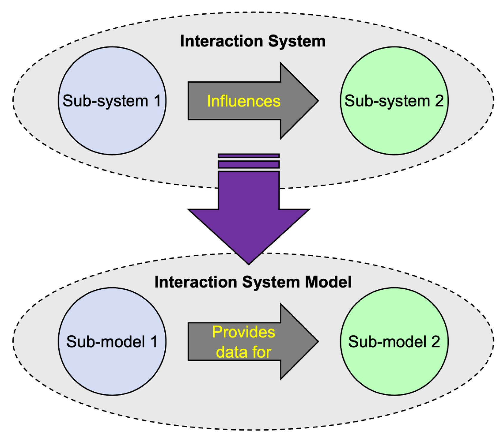
• Both modeling techniques are designed to decompose a full system model into sub-models and coordinate interaction between sub-models as a way of modeling dynamics of the full system rather than using a non-composed model (i.e., a single, all-encompassing model).
• Both techniques are commonly used to capture systems with sub-systems of differing scales and/or from differing domains in which dynamics from one scale or domain propagate affect one or more other scales or domains.

Additionally, the analysis provided in this paper may be used in conjunction with any of the previously proposed complexity measures discussed above. We provide a discussion on the compatibility of our analysis with previously studied complexity measures in Section 8.

3. Composable Modeling Methods: Motivations and Benefits

Interaction systems are characterized by the collective dynamics of two or more interacting sub-systems in which effects originating from at least one sub-system influence the dynamics of one or more other sub-systems. Sub-systems may represent different scales and/or different domains of the whole system. Furthermore, the collective dynamics of the full system are often characterized by inherent uncertainty [1].

A cyber–physical–social system (CPSS) is an interaction system in which deep interactions between human actions and technical/engineering system(s) exist [4,5]. Consider the notional CPSS depicted in Figure 1. The CPSS in the figure represents a generic manufacturing company that utilizes a cyber–physical system to produce one or more items: (1) the organizational behavior of the company (upper left) governs the items produced and the process by which they are produced, (2) the production process (lower left) specifies the details of the production process, (3) the cyber–physical network (upper right) provides the engineering system that executes the production process, and (4) the cyber–physical network software (lower right) captures the software layer of the network that monitors and regulates online production execution. Cyber attack and defense (middle of the figure) dynamics are also part of the whole system and influence all sub-systems.

Modeling and simulation of an interaction system with inherent uncertainty, such as the one given in Figure 1, entails the capture of probabilistic dynamics across domains of human behavior, manufacturing/production engineering, and cyberspace. Additionally, any of the domains may include dynamics that interact over multiple scales. For example, a model of organizational behavior may necessitate the capture of dynamics at the individual, group, and organization-wide scales; a model of the cyber–physical network may require dynamics at the device and network scales; a model of the production process may include dynamics of sub-processes that produce components that are later assembled to produce a complete item.

There are several disadvantages to modeling an interaction system by way of a single, all-encompassing (i.e., non-composed) model.

• High Resource Cost—Modeling all dynamics in a single model requires implementing sub-system dynamics from scratch for all sub-systems, unless there exists an already implemented model capable of capturing all dynamics relevant to the interaction system in question. In-house implementation may require significant engineering, modeling, and domain expertise, as well as a significant amount of time. If such a model already exists commercially, the access cost is also likely to be expensive. In either case, the cost may be prohibitive.
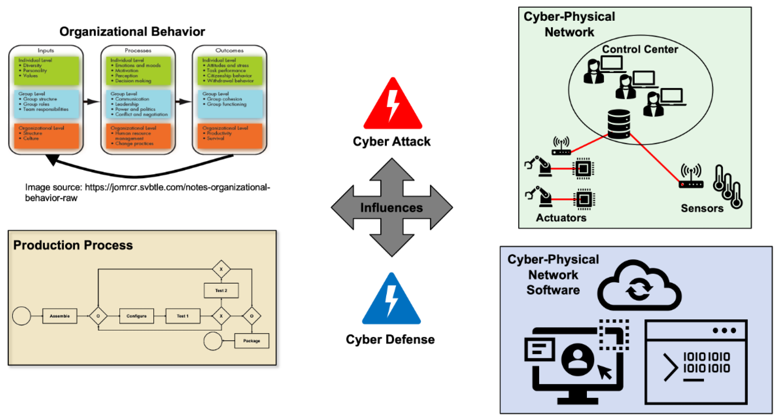
• Lack of Reusability/Extensibility—Multi-scale/multi-domain dynamics interwoven into a single model are often highly customized to the original problem and the addition of new dynamics or alterations to existing dynamics may require significant effort to integrate and test. For example, for the CPSS depicted in Figure 1, if the organization wishes to change the production process model, then this may entail changes to the cyber–physical network and software models. If all models are implemented in a single model, significant re-implementation may be necessary to integrate all changes. Ideally, a modeling approach should readily support model extensibility and reuse to minimize re-implementation costs when changes or additions are desired.
• Lack of Maintainability/Testability—Complex interwoven dynamics across multiple scales and/or domains makes testing and maintenance problematic. Unit tests focusing on individual scales require the inclusion of aspects from other scales. It may be hard to isolate sub-system dynamics and test their individual behaviors. For non-trivial systems, it can be difficult to verify that model implementation matches the intended design.

Composable modeling approaches seek to address these disadvantages by leveraging modularity concepts that are analogous to those of modular software design. The idea is to divide a complex system model into component models that are loosely interdependent. Loose coupling, as its called in the software engineering community, refers to components that are less dependent on each other, such that changes to one component have relatively lesser effects on other components [52]. Note that a non-composed model is one that is not divided into component models, where sub-system dynamics are interwoven and thus tightly interdependent. The significant advantages of composable modeling approaches are recognized by [53].

Composable modeling approaches ameliorate the aforementioned disadvantages in the following ways.

• Reduced Resource Cost—Full system models may be constructed by combining multiple sub-system models potentially originating from disparate sources. For example, a full model of the CPSS in Figure 1 could be constructed by combining pre-existing models of organizational behavior and production processing with custom-made models for the cyber–physical network and its underlying software layer. The ability to leverage existing sub-system models to compose a new full system model significantly reduces the time and domain expertise required to model a complex interaction system. Additionally, loosely interacting component models provide the opportunity for parallel model development, which can further reduce the time required to build a full system model.
• Increased Reusability/Extensibility—Models can be be more easily reused and/or altered due to their loose coupling. For example, for the CPSS in Figure 1, if a new cyber attack exploiting a particular software vulnerability is to be incorporated into to the full system model, it may only be necessary to alter the cyber–physical network software component model without changing other component models. If a software component model capturing the new cyber attack already exists, it potentially may be used in place of the previous software component model. The ability to combine and re-combine existing component models into new full-system models makes for increased model flexibility and adaptability.
• Increased Maintainability/Testability—Loose interdependence supports greater isolation of sub-system dynamics and makes unit testing and model code maintenance relatively easier than tight interdependence.

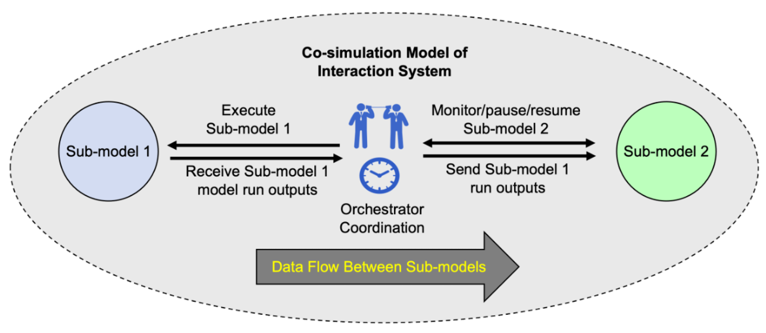
4. Composable Modeling Techniques

As mentioned in Section 1, co-simulation and closure modeling are two prevalent techniques for building composed simulation models of interaction systems [10,18,20,24]. Co-modeling is another composable modeling technique that is closely related to co-simulation in which a unified language is used to specify sub-system models [10,54]. This distinction does not impact the analysis of this paper, and thus, we consider co-modeling and co-simulation as the same technique.

The purpose of this section is to provide a brief description of these two composable modeling techniques by way of a notional, illustrative example. Consider an abstracted interaction system containing two sub-systems in which the dynamics of one sub-system influence the dynamics of the other sub-system and in which inherent uncertainty is present. The two sub-systems may represent different relevant scales or domains of the full system. The abstracted system could, for example, represent a cyber network system in which individual cyber device dynamics influence the dynamics of the network as a whole. As another example, the system could represent a traffic flow system in which dynamics at intersections influence the larger wide-area traffic flow. This simple abstracted system may be applicable to many examples from various domains. A depiction of this notional interaction system and a high-level, generalized depiction of a composed model of this system are given in Figure 2. In the figure, the upper ellipse depicts the notional interaction system, which is made up of Sub-system 1 and Sub-system 2, and in which Sub-system 1 dynamics influence those of Sub-system 2. The lower ellipse depicts a generalized composed model of the interaction system in the upper ellipse. In the lower ellipse, Sub-model 1 represents a model capturing dynamics of the influencing Sub-system 1 while Sub-model 2 captures dynamics of Sub-system 2, which is influenced by Sub-system 1 dynamics. Note that in the composed model, influence is propagated by way of a data exchange from Sub-model 1 to Sub-model 2.

Co-simulation modeling employs an orchestrator component that serves to coordinate model execution and data exchange between sub-models. Figure 3 depicts a co-simulation approach to modeling the interaction system of Figure 2. In the figure, the orchestrator component controls the execution of sub-models to synchronize their data exchange at appropriate times. The orchestrator monitors Sub-model 2 and pauses its execution when an influencing dynamic is required from Sub-model 1. It then executes/re-executes Sub-model 1, receives its outputs, provides these to Sub-model 2, and resumes Sub-model 2 execution. This process may be repeated multiple times during the simulation whenever Sub-model 1 dynamics are required by Sub-model 2.

Closure modeling executes influencing sub-models before their corresponding receiving sub-models. Figure 4 depicts a closure modeling approach for capturing our interaction system example. In the figure, a set of runs is executed on Sub-model 1 and its outputs are aggregated. These aggregations are then used to specify inputs for Sub-model 2. Finally, a set of runs is executed on Sub-model 2.

Note that co-simulation synchronizes the execution and data exchange of sub-models dynamically. This means that sub-model executions are interwoven, at times running in parallel but marked by points in time where one or more sub-models are paused while waiting for other sub-models to execute. Closure modeling, contrary to co-simulation, executes sub-models serially. Influencing sub-models are executed to completion before their corresponding receiving sub-models are executed. Once a sub-model is fully executed (e.g., via a set of runs) it is not re-executed/resumed at a later point in the simulation.

Co-simulation has been widely used in the engineering [10] and cyber–physical system [10,55] problem domains. DEVS-based co-simulation models have been frequently applied for these domains both in a strict sense, where all component models are DEVS models and in a hybrid sense, where DEVS component models interact with non-DEVS component models [56,57,58,59,60]. Closure modeling has been frequently used in the physics [19,20,22,23,24] and cyber security [21,61] problem domains.

5. Foundations

To start, we consider the two-component interaction system and its corresponding model depicted in Figure 2. We will analyze this simplified composed model and then extend and generalize our analysis to more complex models. This section provides foundational specifications and assumptions that will be used throughout the analysis. As shown in the lower ellipse of the figure, the interaction system model contains two sub-models in which Sub-model 1 provides data for Sub-model 2. The combined output of both sub-models, including their data interaction, provides the output for the full model.

For our simplified system, we specify two outcomes of interest, $O_1$ and $O_2$, that are subject to uncertainty. We define an experiment on the system as a single system execution resulting in a pair of outcomes where each outcome is evaluated and results as either true or false. We define two random binary variables $V_1$ and $V_2$ which respectively map outcomes $O_1$ and $O_2$ to the value of 1.0 when the outcome is true and the value of 0.0 when the outcome is false.

We specify system inputs by two vectors of random variables, $\mathit{X}=\langle X_1,\dots ,X_i\rangle$ and $\mathit{Y}=\langle Y_1,\dots ,Y_j\rangle$, where $\mathit{x}$ and $\mathit{y}$ are vectors representing a single sampling taken from $\mathit{X}$ and $\mathit{Y}$, respectively. hlNote that the type of random variable used as system input, e.g., discrete or continuous, does not affect this analysis. System outcomes $O_1$ and $O_2$ are generated by an unknown non-linear function h and mapped to real values by random variables $V_1$ and $V_2$, respectively, such that

$$v_1,v_2=h(\mathit{x},\mathit{y}),$$

(1)

where $v_1$ and $v_2$ represent a single generation of output variables $V_1$ and $V_2$, respectively, as generated by function h with input vectors $\mathit{x}$ and $\mathit{y}$. The system outcomes generated by h are approximated by a system model M:

$$M(\mathit{x},\mathit{y})\approx h(\mathit{x},\mathit{y}),$$

(2)

where $\mathit{x}$ and $\mathit{y}$ are input parameters of M. Note that M is a full, non-composed model of our simplified system without consideration of sub-models or their composition.

We now specify the two sub-models of our system model. We specify that Sub-system 1 (left of upper ellipse in Figure 2) generates outcome $O_1$ via an unknown non-linear function g, such that

$$v_1=g\left(\mathit{x}\right),$$

(3)

where $v_1$ and $\mathit{x}$ are as defined in Equation (1). The sub-system 1 outcome generated by g is approximated by Sub-model 1 (left of lower ellipse in Figure 2), which, for simplicity, we refer to as $M_1$:

$$M_1\left(\mathit{x}\right)\approx g\left(\mathit{x}\right),$$

(4)

where $\mathit{x}$ is an input parameter of $M_1$.

Similarly, we specify that Sub-system 2 (right of upper ellipse in Figure 2) generates outcome $O_2$ via an unknown non-linear function f such that

$$v_2=f(\mathit{y},v_1)$$

(5)

where $v_2$ and $\mathit{y}$ are as defined in Equation (1) and $v_1$ is the output generated by function g (Equation (3)) and approximated by $M_1$ (Equation (4)). The sub-system 2 outcome generated by f is approximated by Sub-model 2 (right of lower ellipse in Figure 2), which, for simplicity, we refer to as $M_2$:

$$M_2(\mathit{y},v_1)\approx f(\mathit{y},v_1),$$

(6)

where $v_1$ is the output approximated by $M_1$ and $\mathit{y}$ and $v_1$ are input parameters of $M_2$.

The above equations formally specify a single experiment for individual models M, $M_1$, and $M_2$ without consideration of sub-models, their interactions, or their composition to create a composed model of our simplified system. For a probabilistic model, it is necessary to execute a set of experiments to sample the distribution of possible model outcomes and estimate their expected values. We wish to compute an outcome distribution via a set of experiments on our composed model given a specification for its input parameters $\mathit{X}$ and $\mathit{Y}$. To this end, we provide the following foundational definitions.

Definition 1 (Experiment Set Size, $\mathit{S}$).

The experiment set size, $S_a$, is the number of experiments executed on a given probabilistic model a.

Definition 2 (Computation Time, $\mathit{T}$).

The computation time, $T_a$, is the time taken to compute a set of experiments on probabilistic model a with experiment set size $S_a$.

Definition 3 (Dynamics Set, $\mathit{\delta }$).

The dynamics set, ${\delta }_a$, is the set of dynamics captured by a given probabilistic model a.

Definition 4 (Complexity, $\mathit{C}$).

The complexity, $C_a$, is a measure of complexity for a given probabilistic model a, where higher values represent greater model complexity.

Note that to accurately estimate the expected value of an outcome for a given probabilistic model, it is necessary to execute a sufficient number of experiments [62,63]. Thus, the experiment set size, S, should be specified appropriately so as to properly characterize the outcome distribution. Also note that S, the experiment set size, and T, the computation time for executing an experiment set of size S, may be used to describe the execution of multiple simulation trials, such as in Monte Carlo simulation, or the execution of a single simulation for a duration of simulated time, such as in continuous-time Markov Chain models. In either case S represents the number of input samples used to generate the outcome distribution and T represents the computation time required to generate the outcome distribution.

Building on the previous works of [64,65] that seek to define simulation model complexity, Thompson [32] characterizes complexity in terms of a model’s scope, resolution, interactions, and logical dependencies. Thompson’s framework proposes that greater scope, more granular/precise resolution, a greater number of interactions, and more logical dependencies are the pertinent factors that contribute to an increase in model complexity.

From Thompson’s framework, given that model complexity is increased with greater model scope (i.e., a greater number of real-world components modeled) and/or finer resolution (i.e., more granular discretization of model parameters and structure), it is reasonable to expect that the model execution time is similarly affected. Similarly, given that complexity also increases with greater numbers of interactions and/or logical dependencies, it is reasonable to expect that an increase in the set of dynamics captured by a given model would entail an increase in the model’s complexity.

Leveraging this framework, we make the following assumptions about the relationship between S, T, $\delta$, and C.

Assumption 1.

1A The computation time necessary to sufficiently execute a given probabilistic model is directly proportional to the model’s complexity. That is, $T_a=l·C_a,l\ge 1$, where $C_a$ is the complexity of model a, $T_a$ is the computation time required to execute a sufficiently sized set of experiments on a, and l is a proportionality constant.

Assumption 2.

1B The complexity of a given probabilistic model is directly proportional to the set of dynamics captured by the model. That is, for two models, a and b, ${\delta }_a\subset {\delta }_b\Rightarrow C_a<C_b$.

Assumption 3.

1C The computation time necessary to execute a given set of experiments is directly proportional to the experiment set size. That is, for a given model a, $T_a=k·S_a,k\ge 1$, where $T_a$ is the computation time required to execute an experiment of size $S_a$ on model a and k is a proportionality constant.

Based on Assumptions 1–3, the following transitive assumption can be deduced.

Assumption 4.

1D The addition of one or more new dynamics to the set of dynamics captured by a model incurs an increase in the computation time necessary to sufficiently execute that model. That is, for two models, a and b, ${\delta }_a\subset {\delta }_b\Rightarrow T_a<T_b$.

For a composed model consisting of two or more sub-models, we make the following assumptions concerning the sets of dynamics captured by each sub-model.

Assumption 5.

2A Every sub-model of a composed model captures at least one dynamic, that is

$$|{\delta }_{m_i}| >0,\forall m_i\in m,$$

where m is a full composed model and $m_i$ represents a sub-model of m.

For our simplified interaction system model M (Equation (2)) with sub-models $M_1$ and $M_2$ (Equations (4) and (6), respectively), Assumption 5 implies $|{\delta }_{M_1}|,|{\delta }_{M_2}| >0$.

Assumption 6.

2B For a composed model consisting of two or more sub-models, no dynamics are duplicated in two or more sub-models. That is,

$${\delta }_{m_i}\cap {\delta }_{m_j}=\varnothing ,\forall m_i,m_j\in m,m_i\ne m_j,$$

where m is a full composed model and $m_i,m_j$ represent sub-models of m.

For our simplified model M, Assumption 6 implies ${\delta }_{M_1}\cap {\delta }_{M_2}=\varnothing$.

For a model that is composed of two or more sub-models, interactions between sub-models produce dynamics in the greater model as a whole. To capture this phenomenon, we introduce the notion of a set of interacting dynamics between two sub-models as a set of pairs of single dynamics from each sub-model which, when executing together, capture greater dynamics of the model as a whole. By executing together, we mean that the two sub-models execute either simultaneously or in an interleaved fashion. We provide the following definitions and assumptions concerning interacting dynamics between sub-models of a composed model.

Definition 5 (Interacting Dynamics Set, $𝙁$).

The interacting dynamics set, ${𝙁}_{{\delta }_a,{\delta }_b}$, is the set of pairs of dynamics between two given probabilistic sub-models, a and b, that execute together to capture combined dynamics not captured in either sub-model’s dynamics set, that is, not captured in either ${\delta }_a$ or ${\delta }_b$. ${𝙁}_{{\delta }_a,{\delta }_b}$ contains tuple elements given by $\langle {\delta }_{a_i},{\delta }_{b_j}\rangle$ where ${\delta }_{a_i}$ and ${\delta }_{b_j}$ are single dynamics from models a and b, respectively.

Assumption 7.

3A If a composed model contains two sub-models, a and b, that execute together, and a influences (provides data for) b, then the set of interacting dynamics between a and b is non-empty. That is

$$a\to b\Rightarrow {𝙁}_{{\delta }_a,{\delta }_b}\ne \varnothing ,$$

(7)

where $a\to b$ represents the influence from a to b.

We define a notion of dense interaction between two sub-models as the maximal possible interaction involving all dynamics captured by both sub-models.

Definition 6 (Dense Interaction).

Two sub-models of a composed model have dense interaction if, when executed together, there is interaction between all possible pairs of single dynamics from each sub-model. That is, for sub-models a and b

$${𝙁}_{{\delta }_a,{\delta }_b}={\delta }_a\times {\delta }_b\Rightarrow dense(a,b),$$

(8)

where ${\delta }_a\times {\delta }_b$ is the cartesian product of sets ${\delta }_a$ and ${\delta }_b$, and $dense(a,b)$ is a function that, for sub-models a and b, maps to the boolean value of true if a and b have dense interaction and false otherwise.

Assumption 8.

3B Two sub-models that do not interact can be executed independently with total complexity that is equivalent to the sum of complexities of each sub-model. That is, for a given model a composed of sub-models b and c,

$${𝙁}_{{\delta }_b,{\delta }_c}=\varnothing \Rightarrow C_a=C_b+C_c,$$

(9)

where $C_a$, $C_b$, and $C_c$ are the complexities of models a, b, and c, respectively, and ${𝙁}_{{\delta }_b,{\delta }_c}$ represents the set of interacting dynamics between sub-models b and c. In other words, independent and non-interacting sub-models do not incur any additional complexity as a result of their interaction.

Assumption 9.

3C Two sub-models executing together with dense interaction have maximal additional complexity due to their interaction relative to the total complexity given by their independent execution without interaction. We characterize this maximal additional complexity as multiplicative with respect to the complexity of their independent execution. That is, for a given model a composed of sub-models b and c

$$dense(b,c)\Rightarrow C_a=C_b·C_c,$$

(10)

where $C_a$, $C_b$, and $C_c$ are as given in (9) and $dense(b,c)$ represents dense interaction between sub-models b and c.

Assumption 10.

3D For two sub-models executing together that do interact, the complexity of their combined execution is greater than the sum of complexities of each sub-model due to the additional complexity given by their interaction. That is, for a given model a composed of sub-models b and c

$${𝙁}_{{\delta }_b,{\delta }_c}\ne \varnothing \Rightarrow C_a>C_b+C_c,$$

(11)

where $C_a$, $C_b$, $C_c$, and ${𝙁}_{{\delta }_b,{\delta }_c}$ are as given in (9). In other words, interacting sub-models incur additional complexity as a result of their interaction relative to the total complexity given by their independent execution without interaction.

6. Analysis of a Simple System Model

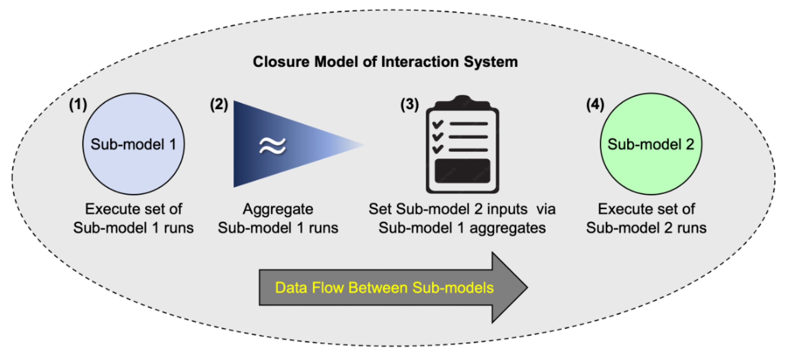
With the formal foundation of the previous section in place, we now consider a fully composed model of our simplified interaction system (Figure 2, Section 4). We will analyze and compare the complexity and computational efficiency of a composed model constructed by the co-simulation approach with that constructed by the closure modeling approach.

We start with the co-simulation approach. Let $M_{cosim}$ be a full, composed model of the simplified system as constructed by the co-simulation modeling approach. A single experiment on $M_{cosim}$ is thus given by

$$v1,v2=M_{cosim}(\mathit{x},\mathit{y}),$$

where $\mathit{x},\mathit{y}$ are input parameters to $M_{cosim}$ as given in Equations (1) and (2) and $v1,v2$ are outputs generated by $M_{cosim}$ as given in the same equations. Because $M_{cosim}$ is a composed model, it thus contains sub-models $M_1$ and $M_2$ (Equations (4) and (6), respectively) where $M_1$ provides data for $M_2$, that is $M_1\to M_2$. Let ${\mu }_{v_1}$ and ${\mu }_{v_2}$ be the expected values of $v_1$ and $v_2$, respectively, as aggregated over a set of experiments executed on a full model of our simplified system. To analyze the computational efficiency of $M_{cosim}$, we wish to specify bounds on $T_{M_{cosim}}$, the total computation time required to execute the set of experiments on $M_{cosim}$ that estimate ${\mu }_{v_1}$ and ${\mu }_{v_2}$.

First, we consider a lower bound. According to Assumption 8, the total complexity of a model composed of sub-models $M_1$ and $M_2$ if there was no interaction between them is given by the sum of their individual complexities. Because these sub-models execute together and do interact, Assumption 10 applies:

$$C_{M_{cosim}}>C_{M_1}+C_{M_2},$$

(12)

where $C_{M_1}$ and $C_{M_2}$ are the complexities for sub-models $M_1$ and $M_2$, respectively, and $C_{M_{cosim}}$ is the complexity of composed model $M_{cosim}$. From Assumption 1 it follows that

$$T_{M_{cosim}}>T_{M_1}+T_{M_2},$$

(13)

where $T_{M_1}$ and $T_{M_2}$ are the computation times for sub-models $M_1$ and $M_2$, respectively, and $T_{M_{cosim}}$ is the computation time of composed model $M_{cosim}$.

To compute the upper bound, we consider the case of dense interaction between $M_1$ and $M_2$, where dense interaction is as given by Definition 6. Dense interaction specifies maximal additional complexity due to interactions between sub-models that execute together relative to the total complexity when no interaction is present. Assumption 9 thus applies, yielding

$$C_{M_{cosim}}\le C_{M_1}·C_{M_2},$$

(14)

where $C_{M_{cosim}}$, $C_{M_1}$, and $C_{M_2}$ are as given in Equation (12). Similar to the lower bound analysis, from Assumption 1, it follows that

$$T_{M_{cosim}}\le T_{M_1}·T_{M_2},$$

(15)

where $T_{M_{cosim}}$, $T_{M_1}$, and $T_{M_2}$ are as given in Equation (13).

Now, we move to the closure modeling approach. Let $M_{closure}$ be a full, composed model of the simplified system, as constructed by the closure modeling approach. Similar to the analysis of $M_{cosim}$, we wish to compute $T_{M_{closure}}$, the total computation time needed to execute the set of experiments on $M_{closure}$ that estimate ${\mu }_{v_1}$ and ${\mu }_{v_2}$.

Recall from Section 4 that closure modeling executes sub-models in series with influencing sub-models executing to completion before receiving models are executed. Data exchange occurs via an aggregation of influencing sub-model outputs, which are then used to set receiving sub-model inputs. Execution of the $M_{closure}$ for our simplified system is thus given by the following steps.

• Model inputs $\mathit{X}$ and $\mathit{Y}$ are specified.
• A set of experiments with set size $S_{M_1}$ is executed on $M_1$ with input parameters given by $\mathit{X}$.
• The set of experiments executed on $M_1$ generates an output distribution which is aggregated to compute ${\mu }_{v_1}$.
• A set of experiments with set size $S_{M_2}$ is executed on $M_2$ with input parameters given by $\mathit{Y}$ and the computed ${\mu }_{v_1}$.
• The set of experiments executed on $M_2$ generates an output distribution which is aggregated to compute ${\mu }_{v_2}$.

As can be seen from the above steps, a single set of experiments is executed on $M_1$, followed by the execution of a single set of experiments on $M_2$. Note that $M_1$ and $M_2$ are never executed together either simultaneously or alternately. Thus, the total computation time of the composed closure model is given by

$$T_{M_{closure}}=T_{M_1}+T_{M_2},$$

(16)

where $T_{M_1}$ and $T_{M_2}$ are the computation times of sub-models $M_1$ and $M_2$, respectively, and $T_{M_{closure}}$ is the total computation time of composed model $M_{closure}$. Note that $T_{M_{closure}}$ is directly proportional to $C_{M_{closure}}$, the complexity of $M_{closure}$ (Assumption 1), and thus

$$C_{M_{closure}}=C_{M_1}+C_{M_2},$$

(17)

where $C_{M_1}$ and $C_{M_2}$ are the complexities of sub-models $M_1$ and $M_2$, respectively.

Although sub-models $M_1$ and $M_2$ are not independent and do interact, the complexity of their interaction is nullified by the aggregation of the data provided by $M_1$ to $M_2$. The resulting complexity and thus computation time of the composed model $M_{closure}$ are in the order of that for a composed model consisting of independent sub-models that do not interact. This reduction of model complexity and computation time is not made without a sacrifice to model fidelity. We discuss this tradeoff space further in Section 8. Because model complexity and computation time are assumed to be directly proportional, for brevity, we restrict the focus of the remainder of this analysis to computation time only.

7. Extension to Complex System Models

This section extends and generalizes the analysis of the previous section to composed models that are more complex than the two-sub-system model of the simplified system depicted in Figure 2 and defined in Section 5. The following sections provide additional foundations needed for the extension, describe and analyze four basic patterns found in more complex composed models, and utilize these patterns to provide a generalized algorithm for analysis of composed probabilistic models.

7.1. Additional Foundations

For more complex systems, we extend the two outcomes specified in Section 5 to a vector of outcomes, $\mathit{O}=\langle O_1,\dots ,O_k\rangle ,k\ge 1$ that are subject to uncertainty. We define a corresponding vector of random variables $\mathit{V}=\langle V_1,\dots ,V_k\rangle$ where $V_i$ maps $O_i$ to a value $v_i\in \Re ,\forall i,1\le i\le k$. We define an experiment on the system as a single system execution resulting in a vector of outcomes, $\mathit{o}=\langle o_1,\dots ,o_k\rangle$ which are mapped by $\mathit{V}$ to a vector of real numbers, $\mathit{v}=\langle v_1,\dots ,v_k\rangle$.

We specify system inputs by a vector of random variables, $\mathit{Z}=\langle Z_1,\dots ,Z_l\rangle ,l\ge 1$ (as discussed in Section 5, the type of random variable used as system input, e.g., discrete or continuous, does not affect this analysis), where $\mathit{z}$ is a vector representing a single sampling taken from $\mathit{Z}$. Similar to the specification given in Section 5, system outcomes $\mathit{O}$ are generated by an unknown non-linear function h and mapped to real values by $\mathit{V}$ such that

$$\mathit{v}=h\left(\mathit{z}\right),$$

(18)

which represents a single generation of output vector $\mathit{V}$ as generated by h with input vector $\mathit{z}$. As given in Equation (2), h is approximated by a system model M which represents the full system model. Let ${\mu }_{v_1},\dots ,{\mu }_{v_k}$ be the expected values for outputs $v_1,\dots ,v_k$, respectively, of $\mathit{v}$, as aggregated over a set of experiments executed on the full system model M.

When M is composed of two or more sub-models, we specify that every input variable ${\mathit{Z}}_{\mathit{i}}$ from input vector $\mathit{Z}$ is specified as an input to at least one sub-model. Furthermore, we specify that every output variable ${\mathit{V}}_{\mathit{i}}$ from output vector $\mathit{V}$ is generated as an output by one and only one sub-model. Note that different sub-models may share the same system input variables, but that each system output variable is generated by only a single sub-model.

We introduce the notion of an interaction graph as a graph representing the sub-models and influence relationships that exist within a composed model.

Definition 7 (Interaction Graph, $\Psi$).

An interaction graph ${\Psi }_m$ for a given composed model m is a directed graph ${\Psi }_m=(N,E)$ in which N is a set of nodes representing sub-models of m and E is a set of edges representing influence relationships in which a sub-model x outputs data that another sub-model y ingest as input, where $E\subseteq (x,y)|(x,y)\in N^2,x\ne y$.

Note that the composed model of the simplified system given in Figure 2 is represented by an interaction graph with two nodes and a single edge. In this paper we analyze composed models given by an acyclic interaction graph, that is when $\Psi$ represents a directed acyclic graph. The analysis of composed models with interaction graphs that contain cycles is a topic of future work and discussed in Section 9.

7.2. Sub-Model Interaction Patterns

We describe and analyze four basic patterns of sub-model interaction. These patterns capture possible sub-graphs of an acyclic interaction graph for a given composed model containing two or more sub-models.

Table 1. Four basic patterns of sub-model interaction in an acyclic interaction graph.

Interaction Pattern	Description
Serial Pattern	Sub-model interactions that occur in serial.
Parallel Single Origin Pattern	Sub-model interactions that occur in parallel and start from a single origin sub-model.
Parallel Single End Pattern	Sub-model interactions that occur in parallel and end at a single ending sub-model.
Parallel Single-Origin-And-End Pattern	Sub-model interactions that occur in parallel, start from a single origin sub-model, and end at a single ending sub-model.

provides a list of these basic patterns.

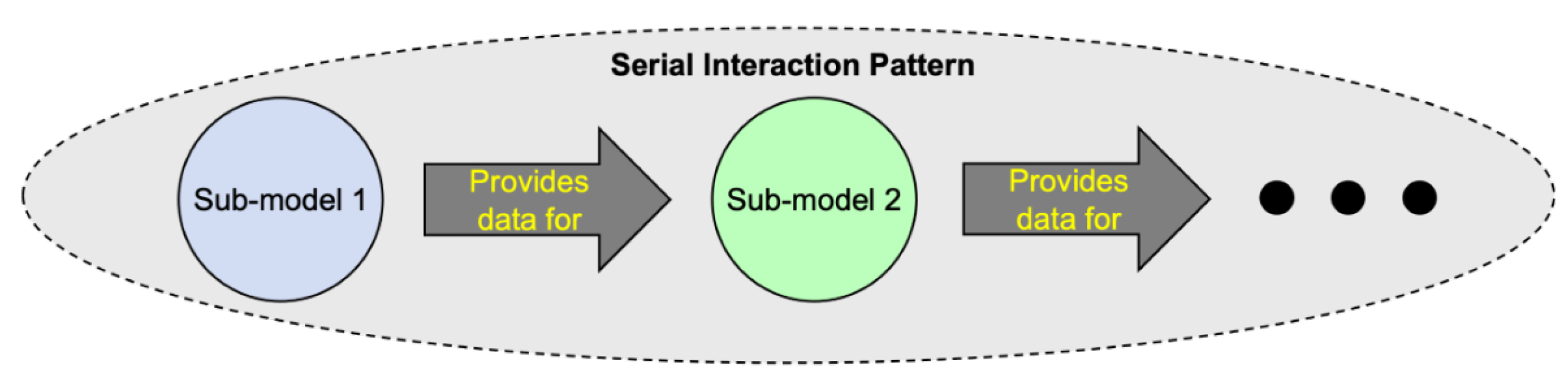
7.2.1. Pattern 1: Interactions in Series

The first pattern captures sub-model interactions that occur in series. The composed model of the simplified system analyzed in Section 5 and Section 6 demonstrates the simplest instance of serial interaction. Figure 5 depicts serial interaction of two or more sub-models. Note that serial interaction implies a directed path on a given interaction graph.

We analyze the co-simulation approach for this serial pattern. Let $M_{cosim}$ be a fully composed co-simulation model consisting of m sub-models and an interaction graph ${\Psi }_M$ with m nodes and $e=m-1$ edges that form a directed path where $m>1$. As for the analysis of Section 6, we wish to specify bounds on $T_{M_{cosim}}$, the total computation time taken to execute the set of experiments on $M_{cosim}$ that estimate aggregated outputs ${\mu }_{v_1},\dots ,{\mu }_{v_k}$.

For the lower bound, leveraging the argument made in Section 6 for co-simulation modeling analysis and generalizing Equation (13) for the serial pattern, we consider the case of m sub-models that do not interact. From Assumption 8, the total complexity of a full model composed of m sub-models that do not interact is given by the sum of their individual complexities. Because the m sub-models do interact, Assumption 10 applies, and together with Assumption 1, it follows that

$$T_{M_{cosim}}>\sum _{i=1}^m{T}_{M_i},$$

(19)

where $T_{M_i}$ is the computation time for sub-model $M_i$ and varies over the m sub-models and $T_{M_{cosim}}$ is the computation time of composed model $M_{cosim}$ for the serial interaction pattern.

For the upper bound, we again leverage the argument of Section 6 for co-simulation analysis by considering dense interaction between sub-model pairs given by the edges of ${\Psi }_M$. From Assumptions 1 and 9, it follows that

$$T_{M_{cosim}}\le \prod _{i=1}^m{T}_{M_i},$$

(20)

where $T_{M_i}$ and $T_{M_{cosim}}$ are as given in Equation (19).

Now, we analyze the closure approach for the serial pattern. Let $M_{closure}$ be a fully composed closure model consisting of m sub-models and the same serial interaction graph ${\Psi }_M$ as described above for the co-simulation analysis. Leveraging the argument made in Section 6 for closure modeling analysis and generalizing Equation (16) for the serial pattern, we have

$$T_{M_{closure}}=\sum _{i=1}^m{T}_{M_i},$$

(21)

where $T_{M_i}$ is the computation time for sub-model $M_i$ and varies over the m sub-models and $T_{M_{closure}}$ is the total computation time of composed model $M_{closure}$ for the serial interaction pattern.

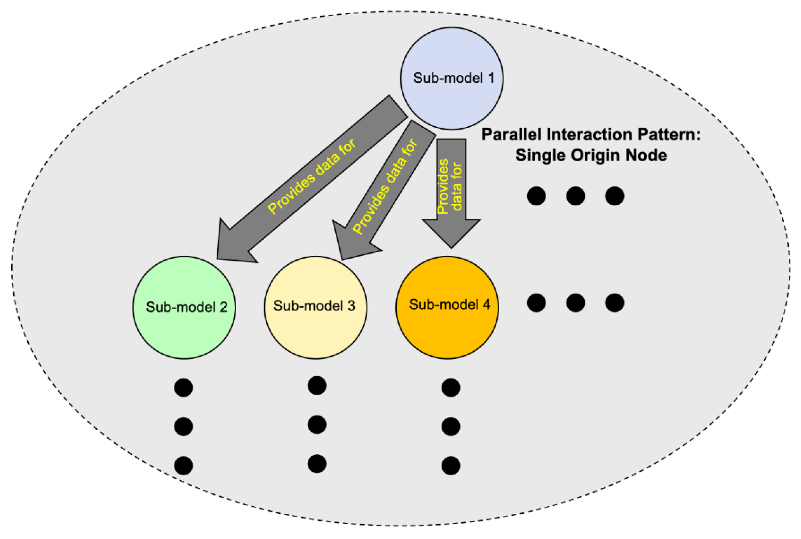
7.2.2. Pattern 2: Parallel Interactions Emanating from a Single Origin Node

This pattern captures sub-model interactions that occur in parallel and emanate from a single origin sub-model. Figure 6 illustrates this pattern. As shown in the figure, parallel interactions from a single origin node in an interaction graph form a tree pattern with the origin node as the root and each directed path representing a branch of the tree. The horizontal dots in the figure represent that there may exist two or more branches in this pattern. The vertical dots in the figure represent the interaction path of each branch, which may consist of two or more nodes. Note that the figure illustrates this pattern by depicting three branches before expansion by horizontal dots. This is not intended to imply that the minimum number of branches is three. Also, the sub-model nodes in the figure are numbered to show that they are unique sub-models only and the numbering is not meant to imply an ordering or total number of nodes.

We analyze the co-simulation approach for this parallel single origin node interaction pattern. Let $M_{cosim}$ be a full composed co-simulation model consisting of m sub-models and an interaction graph ${\Psi }_M$ with m nodes and $e=m-1$ edges that form a directed tree with a single sub-model node as the root. As for the serial pattern analysis of Section 7.2.1, we wish to specify bounds on $T_{M_{cosim}}$. For the lower bound as for the previous lower bound analyses, we consider the case of non-interacting sub-models. Again, Assumptions 1 and 10 apply, yielding the same lower bound as derived for the serial pattern (Equation (19)).

For the upper bound, we consider dense interaction between sub-model pairs given by the edges of ${\Psi }_M$. The tree formed by ${\Psi }_M$ contains two or more branches where each branch is a directed path and thus follows the serial pattern. Let $\mathfrak{B}$ be the set of branches in ${\Psi }_M$. From Assumptions 1 and 9 for a given single branch $\mathfrak{b}\in \mathfrak{B}$ containing a set of sub-model nodes $N_{\mathfrak{b}}$, it follows that

$$T_{\mathfrak{b}}\le \prod _{n\in N_{\mathfrak{b}}}{T}_n,$$

(22)

where n is a sub-model node in $N_{\mathfrak{b}}$, $T_n$ is the computation time of sub-model n, and $T_{\mathfrak{b}}$ is the computation time of branch $\mathfrak{b}$.

The multiple branches of the tree pattern share only an origin/root node. We wish to characterize the combined computation time for these multiple branches, given that they share this origin node. Let $M_{root}$ be the root sub-model node and $M_{child}$ be a given child sub-model node. Recall that, due to the interaction between $M_{root}$ and $M_{child}$, the complexity of their combined execution is greater than the sum of their individual complexities (Assumption 10). Let $\zeta (n_1,n_2)>0$ be the additional complexity due to the interaction between two interacting nodes $n_1$ and $n_2$ that is not accounted for by the sum of these nodes’ individual complexities and let $\tau (n_1,n_2)$ be the corresponding additional computation time (Assumption 1). Thus, the computation time of their combined execution is given by

$$T_{M_{root}\to M_{child}}=T_{M_{root}}+T_{M_{child}}+\tau (M_{root},M_{child})$$

(23)

where $\tau (M_{root},M_{child})$ represents the additional computation time due to the interaction between $M_{root}$ and $M_{child}$ and $T_{M_{root}\to M_{child}}$ is the computation time of the combined execution of $M_{root}$ and $M_{child}$.

Computing the upper bound computation time for an entire interaction tree entails computing the computation time for a single branch via Equation (22) and then computing the computation time of the remaining branches without repeated counting of the root’s computation time, which has already been accounted for in the first branch’s computation. Let ${\mathfrak{b}}_1$ be the first branch of an interaction tree (any branch of the tree may be selected as the first). and $\mathfrak{B}rem=\mathfrak{B}-{\mathfrak{b}}_1$ be the remaining branches of the tree. The computation time of a given remaining branch $\mathfrak{b}rem\in \mathfrak{B}rem$ containing a set of sub-model nodes $N_{\mathfrak{b}rem}$ is given by

$$T_{\mathfrak{b}rem}\le \tau (M_{root},M_{child\in \mathfrak{b}rem})·\prod _{n\in N_{\mathfrak{b}rem},n\ne M_{root}}{T}_n,$$

(24)

where $M_{root}$ is the root sub-model node of the tree, $M_{child}$ is the child node of $M_{root}$ that is also in branch $\mathfrak{b}rem$ (note that there can be only one child of $M_{root}$ that is in a given branch), $\tau (M_{root},M_{child})$ is the additional computation time due to the interaction of $M_{root}$ and $M_{child}$, n is a sub-model node in $N_{\mathfrak{b}rem}$ and varies over all nodes of $N_{\mathfrak{b}rem}$ except the root node $M_{root}$, $T_n$ is the computation time of sub-model n, and $T_{\mathfrak{b}rem}$ is the computation time of a given branch $\mathfrak{b}rem\in \mathfrak{B}rem$.

The upper bound computation time for an entire interaction tree is given by computing the upper bound computation time of an arbitrarily chosen first branch of the tree via Equation (22), computing the upper bound branch computation time of each remaining branch via Equation (24), and summing all computed branch computation times to capture the upper bound computation time of the whole tree. Summation of branch computation times is appropriate because each branch, after interactions with the shared root node have been accounted for, is independent from all other branches with respect to its remaining nodes. That is, no nodes other than the root node are shared between branches. The upper bound computation time for $M_{cosim}$ with interaction graph ${\Psi }_M$ that forms a tree pattern is thus given by

$$T_{M_{cosim}}\le T_{{\mathfrak{b}}_1}+\sum _{\mathfrak{b}rem\in \mathfrak{B}rem}{T}_{\mathfrak{b}rem},$$

(25)

where $T_{{\mathfrak{b}}_1}$ is the computation time an arbitrarily chosen first branch of the tree computed by Equation (22), $\mathfrak{b}rem$ is a remaining branch of the tree and varies over all remaining branches of the tree $\mathfrak{B}rem$, $T_{\mathfrak{b}rem}$ is the computation time of remaining branch $\mathfrak{b}rem$ computed by Equation (24), and $T_{M_{cosim}}$ is the computation time of $M_{cosim}$. Note that the upper bound computation time of Equation (25) sums computation times over branches of the tree, not nodes.

We now analyze the closure approach for this parallel single origin-node pattern. Let $M_{closure}$ be a full composed closure model consisting of m sub-models and the same parallel single origin node interaction graph ${\Psi }_M$ as described above for the co-simulation analysis of this pattern. As described in Section 6 and Section 7.2.1, closure models nullify the added complexity due to dynamic interactions between sub-models by passing aggregated data once instead of non-aggregated data many times. Thus the total computation time for $M_{closure}$ is on the order of that for a model consisting of independent sub-models that do not interact. The computation time is thus given by

$$T_{M_{closure}}=\sum _{i=1}^m{T}_{M_i},$$

(26)

where $T_{M_i}$ is the computation time for sub-model $M_i$ and varies over the m sub-models and $T_{M_{closure}}$ is the total computation time of composed model $M_{closure}$ for the parallel single origin node interaction pattern.

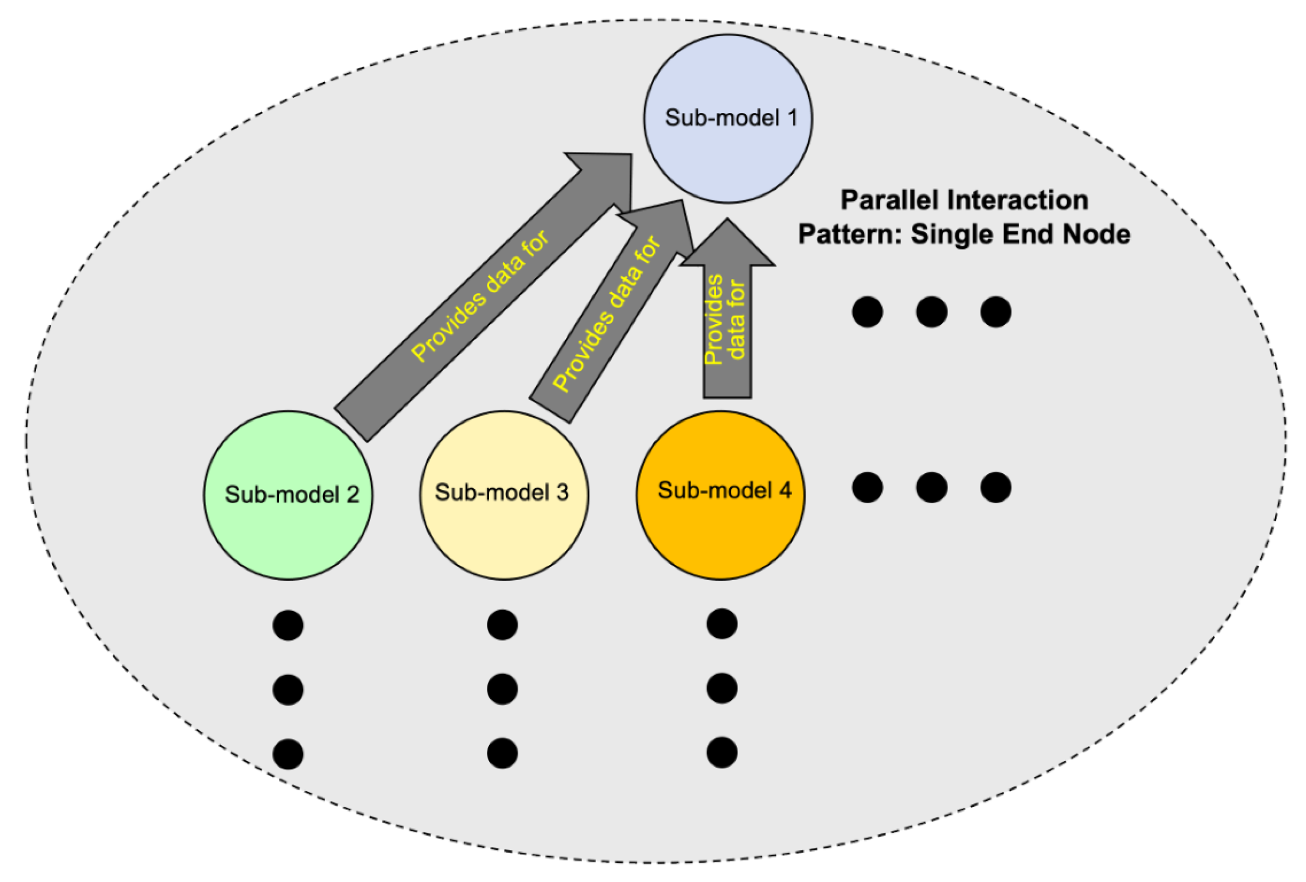
7.2.3. Pattern 3: Parallel Interactions Finishing at a Single End Node

This pattern captures sub-model interactions that occur in parallel and end at a single sub-model node. Figure 7 illustrates this pattern. As shown in the figure, parallel interactions that end at a single node in an interaction graph form a pattern in which two or more directed paths meet at the ending node. The horizontal dots in the figure represent that two or more directed paths may exist in this pattern. The vertical dots in the figure represent the interaction path of each directed path, which may consist of two or more nodes. Note that similar to Figure 6, this figure illustrates the pattern by depicting three paths before expansion by horizontal dots. This is not intended to imply that the minimum number of parallel paths is three. Also, as in Figure 6, the sub-model nodes are numbered only to show that they are unique sub-models and not to imply an ordering or total number of nodes.

We analyze the co-simulation approach for this parallel single end-node interaction pattern. As for the parallel pattern with a single origin-node analysis of Section 7.2.2, we wish to specify bounds on $T_{M_{cosim}}$, the computation time required to compute a composed co-simulation model, $M_{cosim}$, consisting of m sub-models and an interaction graph ${\Psi }_M$ with m nodes and $e=m-1$ edges that form multiple directed paths that terminate at a single end-node. As for the lower bound analysis of the previous two patterns, Assumptions 1 and 10 are used to derive the lower bound given in Equation (19).

As in the analyses of the previous patterns, we consider dense interaction between sub-models to compute the upper bound. Leveraging the analysis of the single origin-node parallel pattern, we use analogous versions of Equations (22) and (24) to compute upper bound computation time for an initial, arbitrarily selected directed path and the same for each individual remaining path without repeated counting of the end node’s computation time. Let $\mathfrak{P}$ be the set of paths in ${\Psi }_M$. From Assumptions 1 and 9 for a given single path $\mathfrak{p}\in \mathfrak{P}$ containing a set of sub-model nodes $N_{\mathfrak{p}}$, it follows that

$$T_{\mathfrak{p}}\le \prod _{n\in N_{\mathfrak{p}}}{T}_n,$$

(27)

where n is a sub-model node in $N_{\mathfrak{p}}$, $T_n$ is the computation time of sub-model n, and $T_{\mathfrak{p}}$ is the computation time of path $\mathfrak{p}$.

As in the analysis of the previous pattern, let $\tau (n_1,n_2)$ be the additional computation time incurred by the combined execution of nodes $n_1$ and $n_2$ that is not accounted for by the sum of their individual computation times. Let $M_{end}$ be the ending node and $M_{parent}$ be a parent/predecessor node. From Equation (23) the computation time of the combined execution of $M_{parent}$ and $M_{end}$ is given by

$$T_{M_{parent}\to M_{end}}=T_{M_{parent}}+T_{M_{end}}+\tau (M_{parent},M_{end})$$

where $\tau (M_{parent},M_{end})$ represents the additional computation time due to the interaction between $M_{parent}$ and $M_{end}$ and $T_{M_{parent}\to M_{end}}$ is the computation time of the combined execution of $M_{parent}$ and $M_{end}$.

Let ${\mathfrak{p}}_1$ be the arbitrarily selected first path of the graph and $\mathfrak{P}rem=\mathfrak{P}-{\mathfrak{p}}_1$ be the remaining paths of the graph. The computation time of a given remaining path $\mathfrak{p}rem\in \mathfrak{P}rem$ containing a set of sub-model nodes $N_{\mathfrak{p}rem}$ is given by

$$T_{\mathfrak{p}rem}\le \tau (M_{parent\in \mathfrak{p}rem},M_{end})·\prod _{n\in N_{\mathfrak{p}rem},n\ne M_{end}}{T}_n,$$

(28)

where $M_{end}$ is the end sub-model node of the graph, $M_{parent}$ is the predecessor node of $M_{end}$ that is also in path $\mathfrak{p}rem$ (note that there can be only one predecessor of $M_{end}$ that is in a given path), $\tau (M_{parent},M_{end})$ is the additional computation time due to the interaction of $M_{parent}$ and $M_{end}$, n is a sub-model node in $N_{\mathfrak{p}rem}$ and varies over all nodes of $N_{\mathfrak{p}rem}$ except the ending node $M_{end}$, $T_n$ is the computation time of sub-model n, and $T_{\mathfrak{p}rem}$ is the computation time of a given path $\mathfrak{p}rem\in \mathfrak{P}rem$.

The upper bound computation time for the entire graph, contrary to that of the single origin-node parallel pattern, is computed by taking a product of the upper bound computation times for each path rather than by taking a sum. Taking a product is appropriate because each path is not independent of the other paths due to their shared ending node, and this dependence cannot be fully accounted for by considering end node interactions with individual paths in isolation as was done for individual branches in the single origin parallel pattern analysis of Section 7.2.2. Because all paths end at the ending node, combined execution of the end sub-model together with the sub-models of each path depends on the combined effects of interacting dynamics between all paths. Similar to our characterization of the complexity and computation time due to dense interaction between two sub-models (Assumption 9), we model the combined interaction of multiple paths multiplicatively.

The upper bound computation time for $M_{cosim}$ with interaction graph ${\Psi }_M$ that follows a pattern with parallel interactions that share a single ending node is thus given by

$$T_{M_{cosim}}\le T_{{\mathfrak{p}}_1}·\prod _{\mathfrak{p}rem\in \mathfrak{P}rem}{T}_{\mathfrak{p}rem},$$

(29)

where $T_{{\mathfrak{p}}_1}$ is the computation time an arbitrarily chosen first path of the graph computed by Equation (27), $\mathfrak{p}rem$ is a remaining path of the graph and varies over all remaining paths of the graph $\mathfrak{P}rem$, $T_{\mathfrak{p}rem}$ is the computation time of remaining path $\mathfrak{p}rem$ computed by Equation (28), and $T_{M_{cosim}}$ is the computation time of $M_{cosim}$.

We now analyze the closure approach for this parallel single end-node pattern. Let $M_{closure}$ be a full composed closure model consisting of m sub-models and the same parallel single end-node interaction graph ${\Psi }_M$ as described above for the co-simulation analysis of this pattern. As described in the previous two sections analyzing the serial and parallel single-origin interaction patterns, closure models nullify interaction complexity by passing aggregated data between sub-models once only. The computation time for $M_{closure}$ is thus the same as that for the parallel single origin-node pattern (Section 7.2.2) and is given by Equation (26).

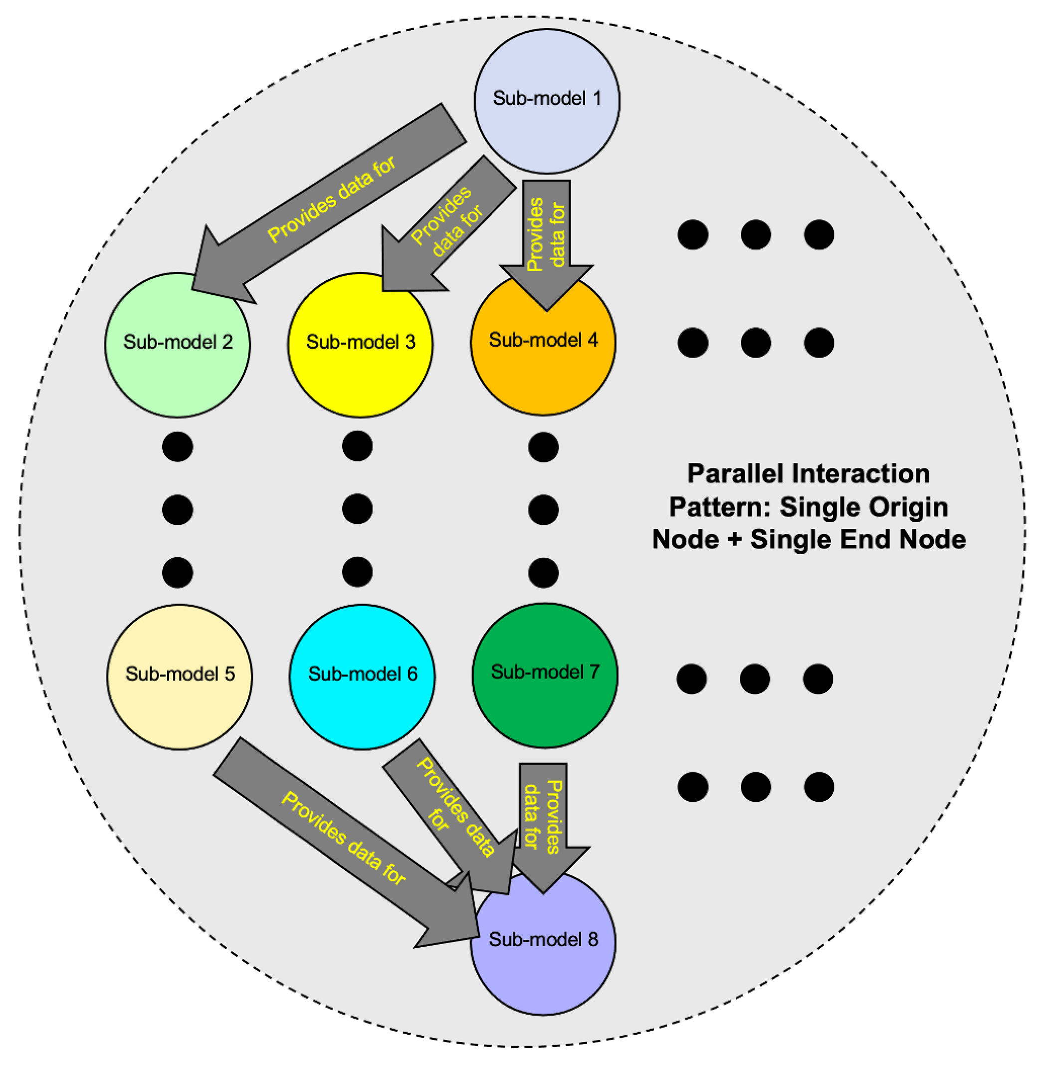
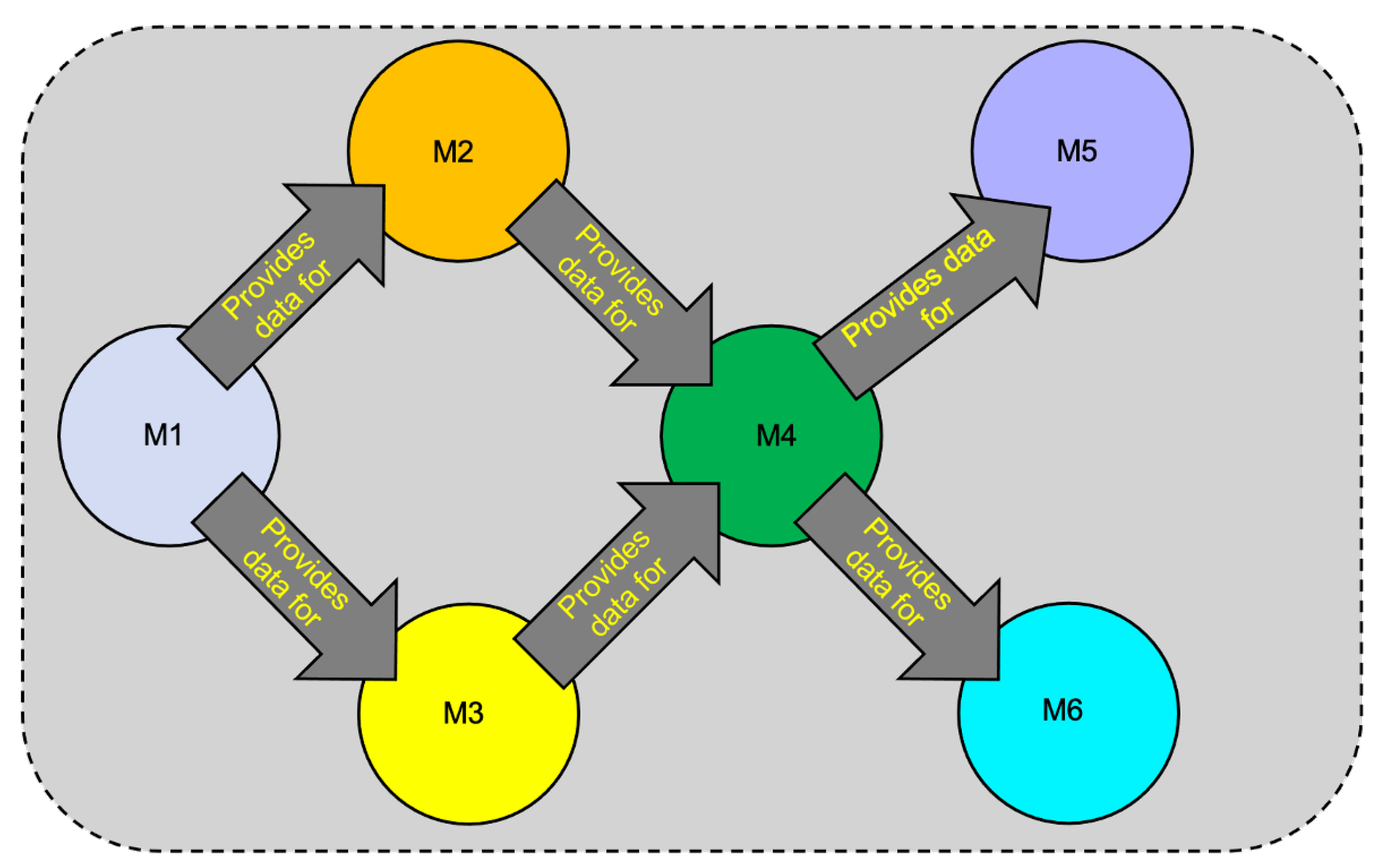
7.2.4. Pattern 4: Parallel Interactions Emanating from a Single Origin-Node and Finishing at a Single End-Node

The final pattern considered is a composite pattern in which sub-model interactions occur in parallel but start from a single origin sub-model node and end at a single end sub-model node. Figure 8 illustrates this pattern. As shown in the figure, parallel interactions with a single origin-node and end-node form a pattern in which two or more directed paths are joined at the start and end nodes. As in Figure 6 and Figure 7, the figure depicts three paths with horizontal dots indicating potentially more paths, but this is not meant to imply that three paths are a minimum. Also, as in the aforementioned figures, numbered nodes represent unique sub-models only and are not meant to imply an ordering or total number of nodes.

We analyze the co-simulation approach for this parallel single-origin-and-end node pattern. As in the previous analyses given in Section 7.2.2 and Section 7.2.3, we specify bounds on $T_{M_{cosim}}$, the computation time to compute a composed co-simulation model, $M_{cosim}$, consisting of m sub-models and an interaction graph ${\Psi }_M$ with m nodes and e edges that form the parallel single-origin-and-end node pattern. Again, as for the lower bound analysis of the previous three patterns, Assumptions 1 and 10 are used to derive the lower bound given in Equation (19).

For the upper bound, we consider dense interaction between sub-models as for the previous analyses. We leverage the analyses of the parallel single origin node and parallel single end node patterns of the previous two sections to compute the upper bound according to the following steps.

• Select either the parallel single origin node pattern (Section 7.2.2) or the parallel single end node pattern (Section 7.2.3) as a starting point for the computation.
• Temporarily ignore either the origin node or end node and its edges depending on which starting pattern is selected. That is, if the parallel single origin node pattern is selected as the starting pattern, then the end node and its edges are ignored. And vice versa if the parallel single end node pattern is selected as the starting pattern.
• Compute the pattern upper bound for the selected starting pattern using the appropriate co-simulation equations for that pattern (equations from either Section 7.2.2 or Section 7.2.3).
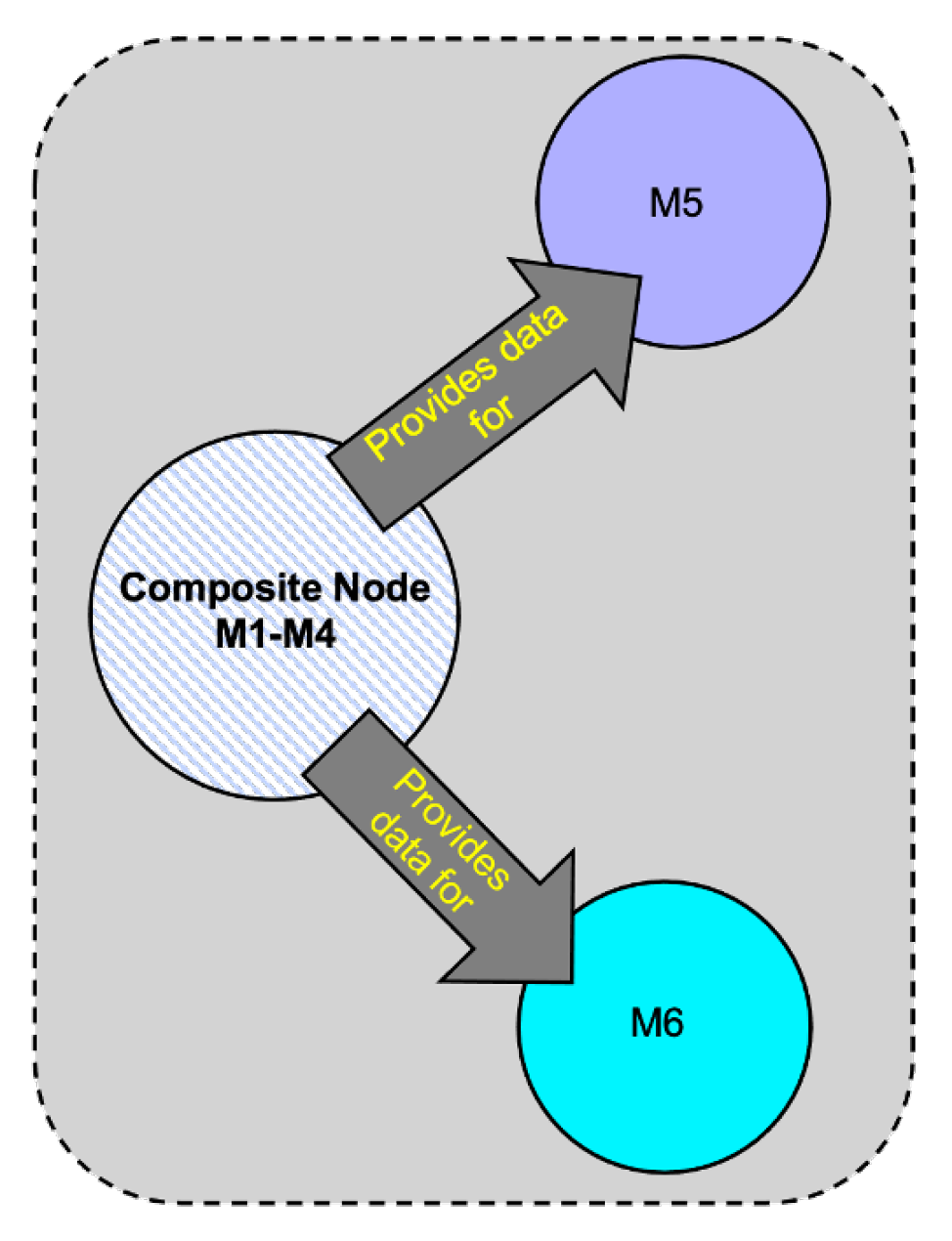
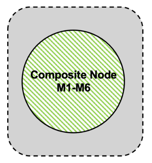
• Collapse all nodes and edges of the starting pattern into a single “composite” node representing the all nodes and edges of that pattern with associated computation time $T_{pattern}$. Note that $T_{pattern}$ represents the upper bound computation time for all nodes and edges of the starting pattern.
• Construct a simpler interaction graph ${\Psi }_{\mathrm{reduced}-M}$ which connects the composite node with the temporarily ignored node by a single edge in the same direction as the previously ignored edges. Note that ${\Psi }_{\mathrm{reduced}-M}$ contains only two nodes and a single edge and is an instance of the serial pattern described in Section 7.2.1.
• Compute the upper bound of ${\Psi }_{\mathrm{reduced}-M}$ using Equation (20) (Section 7.2.1). This upper bound represents the final computation of $T_{M_{cosim}}$ for the original interaction graph ${\Psi }_M$ and is given by

  $$T_{M_{cosim}}\le T_{pattern}·T_n,$$

  (30)

  where $T_{pattern}$ is the computation time for the starting pattern computed in Step 4 above and $T_n$ is the computation time of the remaining temporarily ignored node of ${\Psi }_M$.

The above steps provide the analysis for computing the upper bound given an a priori selection of either the parallel single origin node or parallel single end node pattern as the starting pattern. While an argument can be made for either selection, we prefer to use the parallel single end node pattern as the starting point. Our reasoning is based on the algebraic order of operations in which multiplication is prioritized above addition. Recall from Section 7.2.2 and Section 7.2.3 that the multiple interaction graph paths/branches are combined via a summation for the parallel single origin node pattern and via a product for the parallel single end node pattern.

We now analyze the closure approach for this parallel single-origin-and-end node pattern. Let $M_{closure}$ be a full composed closure model consisting of m sub-models and the same parallel single-origin-and-end node interaction graph ${\Psi }_M$ as described above for the co-simulation analysis of this pattern. As described in the previous analyses of the other patterns, closure models nullify interaction complexity by passing aggregated data. The computation time for $M_{closure}$ is thus the same as that for the parallel single origin node pattern (Section 7.2.2) and is given by Equation (26).

7.3. A Generalized Algorithm

We now provide a generalized algorithm for computing the bounds of computation time T for full composed models constructed by the co-simulation and closure modeling approaches. As mentioned in Section 7, for this analysis we consider an acyclic interaction graph and discuss extension to cyclic interaction graphs in Section 9 as a topic of future work.

We start with the co-simulation approach. As for the pattern analyses given in the previous sections, the lower bound is computed by Equation (19). The upper bound considers dense interaction between sub-model nodes and is computed by Algorithm 1 for a given co-simulation model $M_{cosim}$ with directed acyclic interaction graph ${\Psi }_M$. For simplicity, we consider only connected interaction graphs in the algorithm. For disconnected interaction graphs, the algorithm is used for each connected sub-graph and the final upper bound computation time is given by summing over all individual sub-graph results.

The final result of applying Algorithm 1 on a connected interaction graph is a reduced graph containing a single composite node (no edges) with an associated computation time $T_{pattern}$ representing the total computation time for the graph. To illustrate the application of Algorithm 1, we consider a composed co-simulation model with the interaction graph depicted by Figure 9. As shown in the figure, the composed model consists of six sub-models, labeled as M1–M6, and six edges.

Algorithm 1 General algorithm for computing upper bound computation time of a co-simulation model.

1: procedure Cosim-upper-bound(${\Psi }_M$)                                                                                               ▷ interaction graph ${\Psi }_M$ 2:       for all Pattern 4 sub-graphs (parallel interactions from a single origin node and to a single end node) in ${\Psi }_M$ do 3:             Compute $T_{pattern}$ 4:             Collapse sub-graph into single composite node with associated computation time $T_{pattern}$    ▷${\Psi }_M$ is reduced 5:       for all Pattern 3 sub-graphs (parallel interactions to a single end node) in the reduced graph ${\Psi }_M$ do 6:             Compute $T_{pattern}$ 7:             Collapse sub-graph into single composite node with associated computation time $T_{pattern}$    ▷${\Psi }_M$ is reduced 8:       for all Pattern 2 sub-graphs (parallel interactions from a single origin node) in the reduced graph ${\Psi }_M$ do 9:             Compute $T_{pattern}$ 10:           Collapse sub-graph into single composite node with associated computation time $T_{pattern}$    ▷${\Psi }_M$ is reduced 11:       for all Pattern 1 sub-graphs (serial interactions) in the reduced graph ${\Psi }_M$ do 12:           Compute $T_{pattern}$ 13:           Collapse sub-graph into single composite node with associated computation time $T_{pattern}$    ▷${\Psi }_M$ is reduced

Applying Algorithm 1 to an interaction graph, ${\Psi }_M$, with nodes and edges as depicted in Figure 9, the first step is to compute $T_{pattern}$ for the sub-graph of ${\Psi }_M$ that follows the parallel single-origin-and-end node pattern described in Section 7.2.4. Notice that sub-model nodes M1-M4 together with the four edges connecting nodes M1 and M4 with nodes M2 and M3 form this parallel single-origin-and-end node pattern. Using the steps listed in Section 7.2.4, $T_{pattern}$ for this pattern is computed as

$$T_{pattern}\le T_{M1}·\left(T_{M2}+T_{M4}+\tau (M2,M4)\right)·\left(\tau (M3,M4)·T_{M3}\right),$$

(31)

where $T_{M1},\dots ,T_{M4}$ are the computation times for sub-models M1–M4, respectively, $\tau (M2,M4)$ is the additional computation time due to interaction between sub-models M2 and M4 that is not accounted for by summing their individual computation times, and $\tau (M3,M4)$ is the same for sub-models M3 and M4. Once $T_{pattern}$ is computed, all nodes and edges of the sub-graph are collapsed into a single composite node, where $T_{pattern}$ represents the upper bound computation time of this composite node. After collapsing this sub-graph, the reduced interaction graph is the graph depicted in Figure 10 containing three nodes and two edges. In the figure, the node labeled “Composite Node M1–M4” represents the collapsed sub-graph.

The next step is to compute a new $T_{pattern}$, which we refer to as $T_{pattern}^{\prime }$ for clarity, representing the upper bound computation time of the next prioritized existing pattern on the reduced graph. Notice that the reduced graph of Figure 10 forms an instance of the parallel single origin node interaction pattern described in Section 7.2.2. Also note that there is no instance of the parallel single end node interaction pattern in the reduced graph of Figure 10, therefore we do not consider this pattern in this example. Using Equations (23)–(25) from Section 7.2.2, $T_{pattern}^{\prime }$ is computed as

$$\begin{array}{cc}\hfill T_{pattern}^{\prime }\le & T_{CompositeNode}+T_{M5}+\tau (CompositeNode,M5)\hfill \\ & +\tau (CompositeNode,M6)·T_{M6},\hfill \end{array}$$

(32)

where $T_{M5}$ and $T_{M6}$ are the computation times for sub-models M5 and M6, respectively, $T_{CompositeNode}=T_{pattern}$ is the computation time of the composite node computed in Equation (31), $\tau (CompositeNode,M5)$ is the additional computation time due to interaction between sub-model M5 and the sub-graph containing sub-models M1–M4 represented by the composite node that is not accounted for by summing the individual computation times, $\tau (CompositeNode,M6)$ is the same for sub-model M6 and the composite node. Once $T_{pattern}^{\prime }$ is computed, the nodes and edges of the reduced graph of Figure 10 are collapsed, resulting in the further-reduced graph of Figure 11 containing only a single composite node where $T_{pattern}^{\prime }$ represents the upper bound computation time for the entire original composed co-simulation model.

We now provide a generalized algorithm for computing bounds of computation time T for full composed models constructed by the closure modeling approach. As discussed in the previous sections, the computation time for $M_{closure}$ is computed by summing the individual computation times of each of its sub-models as given by Equation (26) (Section 7.2.2).

Theorem 1.

Given a probabilistic simulation model M composed of two or more probabilistic sub-models whose interactions are given by a directed acyclic interaction graph with two or more nodes and at least one edge, the complexity $C_M$ and computation time $T_M$ of the composed model as constructed by the co-simulation approach are greater than those of the same model as constructed by the closure approach. That is,

$$C_{M_{cosim}}>C_{M_{closure}},T_{M_{cosim}}>T_{M_{closure}},$$

where $M_{cosim}$ and $M_{closure}$ represent the given composed model M as constructed by the co-simulation and closure modeling approaches, respectively, $C_{M_{cosim}}$ and $C_{M_{closure}}$ represent their corresponding complexities, respectively, and $T_{M_{cosim}}$ and $T_{M_{closure}}$ represent their corresponding computation times, respectively.

Proof. 

As given in the above analysis, $T_{M_{cosim}}$ is bounded below by Equation (19) (Section 7), which captures a sum of individual sub-model computation times. As given in the equation, this lower bound is non-inclusive. As given by the above analysis and captured by Equation (26) (Section 7.2.2), $T_{M_{closure}}$ is equal to the sum of individual sub-model computation times. Thus, $T_{M_{closure}}$ is always less than $T_{M_{cosim}}$ for a given composed model with a directed acyclic interaction graph. Because $T_m$ is directly proportional to $C_m$ for any given model m (Assumption 1), $C_{M_{closure}}$ is also always less than $C_{M_{cosim}}$ for a given composed model with a directed acyclic interaction graph. □

8. Discussion

The analysis provided above proves that a composed model constructed by the closure modeling technique has lower complexity and thus higher computational efficiency (i.e., a lower required computation time) than the same model as constructed by the co-simulation technique for composed models with acyclic interaction graphs. It is very important to note that this result does not suggest that closure modeling is preferable to co-simulation. Closure models sacrifice model fidelity to achieve higher efficiency. It is critical to consider trade-offs between model fidelity, computational efficiency, and resource cost when selecting a composable modeling approach. Generally, higher-fidelity models are associated with higher resource costs for model development (or licensing if the model is purchased) and for model execution/use.

For a given modeling application, the selection of a composable modeling approach is driven by the model’s purpose. There are several relevant questions to consider. Is the model intended to capture an existing system or a system that is being designed/modified? If for a system in design, for what design phase is the model intended? If for an existing system, is the model intended to capture system behavior under normal conditions or under abnormal conditions? Is it intended to gain general insights into system behavior or to provide relatively precise predictions of system outcomes?

Early system design modeling applications often wish to compare the relative performance of different design choices, and thus require greater computational efficiency to enable evaluation of numerous options. Later system design applications may wish to simulate full system execution to identify scenarios that cause failure or otherwise unsatisfactory conditions. Thus, these applications may necessitate higher-fidelity models to accurately estimate failure thresholds. Models of an existing system that wish to gain general insights may not require the same fidelity as those that wish to generate predictions of system outcomes. For models that are intended to explore abnormal conditions, for example, to prepare for potential contingencies or system disruptions, evaluating the relative effects of various mitigation strategies may also require greater model efficiency to support what-if analysis of many possible scenarios. Models that are part of a simulation-based optimization/decision support system frequently require rapid simulation execution to enable automated/semi-automated discovery of effective decisions.

Given that physics modeling applications can require capturing interactions between a very large number of entities at the micro-scale (e.g., at the molecular scale) and how these dynamics affect behavior at the macro-scale, it is not surprising that closure models are selected due to their greater efficiency. It may be that for such applications, it is simply intractable to select other modeling approaches.

A limitation of the analysis provided in this paper is that it considers interactions between sub-systems that are acyclic rather than cyclic/bi-directional. However, the analytical approach given here can readily be extended to include cyclic interactions. The analysis of this study is intended to provide the foundation from which analysis of cyclic interactions between sub-systems, as modeled by either the co-simulation or closure modeling approaches, can be developed.

Note that some modeling applications may have a mix of bi-directional/cyclic and unidirectional interactions, that is, some sub-systems that participate in bi-directional/cyclic interactions while other sub-systems participate only in unidirectional interactions. There exists the potential for a hybrid composable modeling approach, where some interaction relationships between sub-systems are captured via a co-simulation technique and others (either bi-directional/cyclic or unidirectional) are captured via a closure modeling technique. Modelers who apply a hybrid composable modeling approach may judiciously select which interaction relationships to model via co-simulation and which to model via closure. This may lead to efficient composable models that are less computationally intensive to execute while remaining accurate for their modeling purpose.

It is also important to note that the above analysis of composable modeling approaches may be used in conjunction with any of the previously proposed complexity measures discussed in Section 2. Our analysis captures the complexity due to interactions that occur between component models of a given interaction system model and does not capture the complexity internal to individual component models. Thus, any desired method may be used to measure the complexity of individual component models and the resulting complexity for the composed model as a whole can be computed using the analysis presented here.

9. Conclusions

This paper presents a probabilistic analysis comparing the complexity and computational efficiency of two prevalent composable modeling techniques, co-simulation and closure modeling. We also discuss the motivations for composable modeling, provide an overview description of the two techniques, discuss trade-offs to consider when selecting an appropriate technique for a given modeling and simulation application, and identify modeling situations that are amenable to either of the composable techniques examined. The aim is to progress the understanding of existing composable modeling techniques and aid modeling practitioners and stakeholders in making informed decisions about the selection of an appropriate modeling technique for a particular modeling application.

Future work could extend the analysis provided here to include composed models with cyclic interaction graphs (Definition 7, Section 7). Intuitively, it can be seen that for a composed model with a cyclic interaction graph, the computational efficiency advantage that closure modeling has over co-simulation may be reduced. Another direction of future work could focus on analyses that provide tighter bounds on the complexity and computational efficiency of co-simulation models.

As discussed by Henriksen in his discourse on complexity in the modeling and simulation community [27], the first mandate of complex systems modelers is to reduce complexity. Composable modeling approaches have been designed explicitly to reduce complexity and are especially appropriate for the multi-scale and multi-domain modeling and simulation problems that are now commonplace. Furthermore, this study points to the potential for a hybrid modeling approach that leverages both the co-simulation and closure modeling techniques. Such an approach enables modelers to judiciously select which interaction relationships between sub-systems to model via a co-simulation technique and which to model via a closure technique. This may lead to efficient composable models that are less computationally intensive to execute while remaining accurate for their modeling purpose.

References

1. Siegenfeld, A.F.; Bar-Yam, Y. An introduction to complex systems science and its applications. Complexity 2020, 2020, 6105872. [Google Scholar] [CrossRef]
2. Thurner, S.; Hanel, R.; Klimek, P. Introduction to the Theory of Complex Systems; Oxford University Press: Oxford, UK, 2018. [Google Scholar]
3. Camus, B.; Bourjot, C.; Chevrier, V. Considering a multi-level model as a society of interacting models: Application to a collective motion example. J. Artif. Soc. Soc. Simul. 2015, 18, 7. [Google Scholar] [CrossRef]
4. Reine, R.; Juwono, F.H.; Sim, Z.A.; Wong, W.K. Cyber-Physical-Social Systems: An Overview. In Smart Connected World: Technologies and Applications Shaping the Future; Springer: Cham, Switzerland, 2021; pp. 25–45. [Google Scholar]
5. Yin, D.; Ming, X.; Zhang, X. Understanding data-driven cyber-physical-social system (D-CPSS) using a 7C framework in social manufacturing context. Sensors 2020, 20, 5319. [Google Scholar] [CrossRef] [PubMed]
6. Doostmohammadian, M.; Rabiee, H.R.; Khan, U.A. Cyber-social systems: Modeling, inference, and optimal design. IEEE Syst. J. 2019, 14, 73–83. [Google Scholar] [CrossRef]
7. Dressler, F. Cyber physical social systems: Towards deeply integrated hybridized systems. In Proceedings of the International Conference on Computing, Networking and Communications (ICNC), Maui, HI, USA, 5–8 March 2018; pp. 420–424. [Google Scholar]
8. Sheth, A.; Anantharam, P.; Henson, C. Physical-cyber-social computing: An early 21st century approach. IEEE Intell. Syst. 2013, 28, 78–82. [Google Scholar] [CrossRef]
9. Baxter, G.; Sommerville, I. Socio-technical systems: From design methods to systems engineering. Interact. Comput. 2011, 23, 4–17. [Google Scholar] [CrossRef]
10. Gomes, C.; Thule, C.; Broman, D.; Larsen, P.G.; Vangheluwe, H. Co-simulation: A survey. ACM Comput. Surv. 2018, 51, 49. [Google Scholar] [CrossRef]
11. Wang, F.; Magoua, J.J.; Li, N. Modeling cascading failure of interdependent critical infrastructure systems using HLA-based co-simulation. Autom. Constr. 2022, 133, 104008. [Google Scholar] [CrossRef]
12. Pedersen, N.; Lausdahl, K.; Sanchez, E.V.; Larsen, P.G.; Madsen, J. Distributed Co-Simulation of Embedded Control Software with Exhaust Gas Recirculation Water Handling System using INTO-CPS. In Proceedings of the 7th International Conference on Simulation and Modeling Methodologies, Technologies and Applications, Madrid, Spain, 26–28 July 2017. [Google Scholar]
13. Oh, S.; Chae, S. A Co-Simulation Framework for Power System Analysis. Energies 2016, 9, 131. [Google Scholar] [CrossRef]
14. Abad, A.-j.G.C.; Guerrero, L.M.F.G.; Ignacio, J.K.M.; Magtibay, D.C.; Purio, M.A.C.; Raguindin, E.Q. A simulation of a power surge monitoring and suppression system using LabVIEW and multisim co-simulation tool. In Proceedings of the International Conference on Humanoid, Nanotechnology, Information Technology, Communication and Control, Environment and Management (HNICEM), Cebu, Philippines, 9–12 December 2015; pp. 1–3. [Google Scholar]
15. Bian, D.; Kuzlu, M.; Pipattanasomporn, M.; Rahman, S.; Wu, Y. Real-time co-simulation platform using OPAL-RT and OPNET for analyzing smart grid performance. In Proceedings of the IEEE Power & Energy Society General Meeting, Denver, CO, USA, 26–30 July 2015; pp. 1–5. [Google Scholar]
16. Elsheikh, A.; Awais, M.U.; Widl, E.; Palensky, P. Modelica enabled rapid prototyping of cyber-physical energy systems via the functional mockup interface. In Proceedings of the Workshop on Modeling and Simulation of Cyber-Physical Energy Systems (MSCPES), Berkeley, CA, USA, 20 May 2013; pp. 1–6. [Google Scholar]
17. Al-Hammouri, A.T. A comprehensive co-simulation platform for cyber-physical systems. Comput. Commun. 2012, 36, 8–19. [Google Scholar] [CrossRef]
18. Cao, Q. Research on co-simulation of multi-resolution models based on HLA. Simulation 2023, 99, 515–535. [Google Scholar] [CrossRef]
19. Roy, D.; Kovalenko, A. Biomolecular Simulations with the Three-Dimensional Reference Interaction Site Model with the Kovalenko-Hirata Closure Molecular Solvation Theory. Int. J. Mol. Sci. 2021, 10, 5061. [Google Scholar] [CrossRef]
20. Baltussen, M.W.; Buist, K.A.; Peters, E.A.J.F.; Kuipers, J.A.M. Multiscale modelling of dense gas—Particle flows. Adv. Chem. Eng. 2018, 53, 1–52. [Google Scholar]
21. Wagner, N.; Sahin, C.S.; Winterrose, M.; Riordan, J.; Hanson, D.; Peña, J.; Streilein, W.W. Quantifying the mission impact of network-level cyber defensive mitigations. J. Def. Model. Simul. 2017, 14, 201–216. [Google Scholar] [CrossRef]
22. Samaey, G.; Lelièvre, T.; Legat, V. A numerical closure approach for kinetic models of polymeric fluids: Exploring closure relations for FENE dumbbells. Comput. Fluids 2011, 43, 119–133. [Google Scholar] [CrossRef]
23. van der Hoef, M.A.; van Sint Annaland, M.; Deen, N.G.; Kuipers, J.A.M. Numerical simulation of dense gas-solid fluidized beds: A multiscale modeling strategy. Annu. Rev. Fluid Mech. 2008, 40, 47–70. [Google Scholar] [CrossRef]
24. van der Hoef, M.A.; van Sint Annaland, M.; Andrews, A.T., IV; Sundaresan, S.; Kuipers, J.A.M. Multiscale modeling of gas-fluidized beds. Adv. Chem. Eng. 2006, 31, 65–149. [Google Scholar]
25. Ahmed, R.; Shah, M.; Umar, M. Concepts of simulation model size and complexity. Int. J. Simul. Model. 2016, 15, 213–222. [Google Scholar] [CrossRef]
26. Stockmeyer, L. Classifying the computational complexity of problems. J. Symb. Log. 1987, 52, 1–43. [Google Scholar] [CrossRef]
27. Henriksen, J.O. Taming the complexity dragon. J. Simul. 2008, 2, 3–17. [Google Scholar] [CrossRef]
28. Arthur, J.D.; Sargent, R.; Dabney, J.; Law, A.M.; Morrison, J.D. Verification and validation: What impact should project size and complexity have on attendant V&V activities and supporting infrastructure. In Proceedings of the WSC’99. 1999 Winter Simulation Conference, Phoenix, AZ, USA, 5–8 December 1999; pp. 148–155. [Google Scholar]
29. Chwif, L.; Barretto, M.R.P.; Paul, R.J. On simulation model complexity. In Proceedings of the 2000 Winter Simulation Conference Proceedings, Orlando, FL, USA, 10–13 December 2000. [Google Scholar]
30. Robinson, S. Modes of simulation practice: Approaches to business and military simulation. Simul. Model. Pract. Theory 2002, 10, 513–523. [Google Scholar] [CrossRef]
31. Ward, S.C. Arguments for constructively simple models. J. Oper. Res. Soc. 1989, 40, 141–153. [Google Scholar] [CrossRef]
32. Thompson, J.S.; Hodson, D.D.; Grimaila, M.R.; Hanlon, N.; Dill, R. Toward a Simulation Model Complexity Measure. Information 2023, 14, 202. [Google Scholar] [CrossRef]
33. Sarjoughian, H.S. Restraining complexity and scale traits for component-based simulation models. In Proceedings of the Winter Simulation Conference (WSC), Las Vegas, NV, USA, 3–6 December 2017; pp. 675–689. [Google Scholar]
34. Yucesan, E.; Schruben, L. Complexity of simulation models: A graph theoretic approach. INFORMS J. Comput. 1998, 10, 94–106. [Google Scholar] [CrossRef]
35. Schruben, L.; Yucesan, E. Complexity of simulation models: A graph theoretic approach. In Proceedings of the 25th Conference on Winter Simulation, Los Angeles, CA, USA, 12–15 December 1993; pp. 641–649. [Google Scholar]
36. Popovics, G.; Monostori, L. An approach to determine simulation model complexity. Procedia CIRP 2016, 52, 257–261. [Google Scholar] [CrossRef]
37. Tolk, A. Interoperability and Composability: A Journey through Mathematics, Computer Science, and Epistemology. In Proceedings of the NATO MSG Symposium, NATO Report STO-MP-MSG-149, Lisbon, Portugal, 19–20 October 2017. [Google Scholar]
38. Davis, P.K.; Anderson, R.H. Improving the composability of DoD models and simulations. J. Def. Model. Simul. 2004, 1, 5–17. [Google Scholar] [CrossRef]
39. Zacharewicz, G.; Diallo, S.; Ducq, Y.; Agostinho, C.; Jardim-Goncalves, R.; Bazoun, H.; Wang, Z.; Doumeingts, G. Model-based approaches for interoperability of next-generation enterprise information systems: State of the art and future challenges. Inf. Syst.-Bus. Manag. 2016, 14, 495–519. [Google Scholar] [CrossRef]
40. Geraci, A. IEEE Standard Computer Dictionary: Compilation of IEEE Standard Computer Glossaries; IEEE Press: New York, NY, USA, 1991. [Google Scholar]
41. Page, E.H.; Opper, J.M. Observations on the complexity of composable simulation. In Proceedings of the 31st Conference on Winter Simulation: Simulation—A Bridge to the Future, Phoenix, AZ, USA, 5–8 December 1999; pp. 553–560. [Google Scholar]
42. Yilmaz, L.; Oren, T.I. Exploring agent-supported simulation brokering on the semantic web: Foundations for a dynamic composability approach. In Proceedings of the 2004 Winter Simulation Conference, Washington, DC, USA, 5–8 December 2004. [Google Scholar]
43. Tolk, A.; Bair, L.J.; Diallo, S.Y. Supporting Network Enabled Capability by extending the Levels of Conceptual Interoperability Model to an interoperability maturity model. J. Def. Model. Simul. 2013, 10, 145–160. [Google Scholar] [CrossRef]
44. Diallo, S.Y.; Padilla, J.J.; Gore, R.; Herencia-Zapana, H.; Tolk, A. Toward a formalism of modeling and simulation using model theory. Complexity 2014, 19, 56–63. [Google Scholar] [CrossRef]
45. Gander, M.J.; Al-Khaleel, M.; Ruchli, A.E. Optimized waveform relaxation methods for longitudinal partitioning of transmission lines. IEEE Trans. Circuits Syst. 2008, 56, 1732–1743. [Google Scholar]
46. Jackiewicz, Z.; Kwapisz, M. Convergence of waveform relaxation methods for differential-algebraic systems. SIAM J. Numer. Anal. 1996, 33, 2303–2317. [Google Scholar] [CrossRef]
47. White, J.A.; Odeh, F.; Vincentelli, A.S.; Ruehli, A.E. Waveform Relaxation: Theory and Practice; Electronics Research Laboratory, College of Engineering, UCB: Berkeley, CA, USA, 1985. [Google Scholar]
48. Bouanan, Y.; Zacharewicz, G.; Vallespir, B. Discrete Event System Specification-Based Framework for Modelling and Simulation of Propagation Phenomena in Social Networks: Application to the Information Spreading in a Multi-Layer Social Network. Simulation 2019, 95, 411–427. [Google Scholar] [CrossRef]
49. Sanz, V.; Urquia, A. Combining PDEVS and Modelica for describing agent-based models. Simulation 2023, 99, 455–474. [Google Scholar] [CrossRef]
50. Tiller, M. Introduction to Physical Modeling with Modelica; Springer Science and Business Media: New York, NY, USA, 2012; Volume 615. [Google Scholar]
51. Xu, X.; Dou, Y.; Ouyang, W.; Jiang, J.; Yang, K.; Tan, Y. A product requirement development method based on multi-layer heterogeneous networks. Adv. Eng. Inform. 2023, 58, 102184. [Google Scholar] [CrossRef]
52. Myers, G.J. Reliable Software through Composite Design; Petrocelli-Charter: New York, NY, USA, 1975. [Google Scholar]
53. Balci, O.; Ball, G.L.; Morse, K.L.; Page, E.; Petty, M.D.; Tolk, A.; Veautour, S.N. Model reuse, composition, and adaptation. In Research Challenges in Modeling and Simulation for Engineering Complex Systems; Springer: Cham, Switzerland, 2017. [Google Scholar]
54. Cellier, F.E.; Kofman, E. Continuous System Simulation; Springer Science & Business Media: New York, NY, USA, 2006. [Google Scholar]
55. Czekster, R.M.; Morisset, C.; Clark, J.A.; Soudjani, S.; Patsios, C.; Davison, P. Systematic review of features for co-simulating security incidents in cyber-physical systems. Secur. Priv. 2021, 4, e150. [Google Scholar] [CrossRef]
56. Camus, B.; Bourjot, C.; Chevrier, V. Combining DEVS with multiagent concepts to design and simulate multi-models of complex systems. In Proceedings of the Symposium on Theory of Modeling and Simulation: DEVS Integrative M&S Symposium. Society for Computer Simulation International, Alexandria, VA, USA, 12–15 April 2015. [Google Scholar]
57. Camus, B.; Galtier, V.; Caujolle, M.; Chevrier, V. Hybrid Co-simulation of FMUs using DEV and DESS in MECSYCO. In Proceedings of the Symposium on Theory of Modeling and Simulation—DEVS Integrative M&S Symposium (TMS/DEVS 16), Pasadena, CA, USA, 3–6 April 2016. [Google Scholar]
58. Denil, J.; De Meulenaere, P.; Demeyer, S.; Vangheluwe, H. DEVS for AUTOSAR-based system deployment modeling and simulation. Simulation 2017, 93, 489–513. [Google Scholar] [CrossRef]
59. Nutaro, J. Designing power system simulators for the smart grid: Combining controls, communications, and electro-mechanical dynamics. In Proceedings of the IEEE Power and Energy Society General Meeting, Detroit, MI, USA, 24–28 July 2011; pp. 1–5. [Google Scholar]
60. Quesnel, G.; Duboz, R.; Versmisse, D.; Ramat, É. DEVS coupling of spatial and ordinary differential equations: VLE framework. In Proceedings of the Open International Conference on Modeling and Simulation, Las Vegas, NV, USA, 27–30 June 2005; Volume 5, pp. 281–294. [Google Scholar]
61. Wagner, N.; Sahin, C.S.; Hanson, D.; Peña, J.; Vuksani, E.; Tello, B. Quantitative analysis of the mission impact for host-level cyber defensive mitigations. In Proceedings of the 49th Annual Simulation Symposium, Pasadena, CA, USA, 3–6 April 2016; pp. 1–8. [Google Scholar]
62. Dekking, F.M.; Kraaikamp, C.; Lopuhaä, H.P.; Meester, L.E. A Modern Introduction to Probability and Statistics: Understanding Why and How; Springer: London, UK, 2005. [Google Scholar]
63. Sawilowsky, S.S. You think you’ve got trivials? J. Mod. Appl. Stat. Methods 2003, 1, 218–225. [Google Scholar] [CrossRef]
64. Davis, P.K.; Hillestad, R. Aggregation, disaggregation, and the challenge of crossing levels of resolution when designing and connecting models. In Proceedings of the 4th Annual Conference on AI, Simulation and Planning in High Autonomy Systems, Tucson, AZ, USA, 20–22 September 1993; pp. 180–188. [Google Scholar]
65. Zeigler, B.P.; Muzy, A.; Kofman, E. Abstraction: Constructing Model Families. In Theory of Modeling and Simulation: Discrete Event & Iterative System Computational Foundations; Academic Press: Cambridge, MA, USA, 2018. [Google Scholar]
Figure 1. An exemplar interaction system: a notional cyber–physical–social system representing the production process of a manufacturing company.
Systems 12 00096 g001
Figure 2. Interaction system with two subsystems (upper ellipse) and a high-level, generalized depiction of a model of the system that is composed of two interacting sub-models (lower ellipse).
Systems 12 00096 g002
Figure 3. Interaction system of Figure 2 as modeled by a co-simulation technique. The orchestrator coordinates the data flow from Sub-model 1 to Sub-model 2.
Systems 12 00096 g003
Figure 4. Interaction system of Figure 2 as modeled by a closure modeling technique.
Systems 12 00096 g004
Figure 5. Serial interaction between sub-models.
Systems 12 00096 g005
Figure 6. Parallel interactions between three or more sub-models that emanate from a single origin sub-model. The horizontal dots represent that there may be two or more branches from the origin node. The vertical dots represent the interaction path of each single branch, which may consist of two or more sub-models.
Systems 12 00096 g006
Figure 7. Parallel interactions between three or more sub-models that all end at a single sub-model node. Horizontal dots represent that there may be two or more paths to the end node. Vertical dots represent the interaction path of each single path, which may consist of two or more sub-models.
Systems 12 00096 g007
Figure 8. Parallel interactions between three or more sub-models that all start from a single origin node and end at a single end node. Horizontal dots represent that there may be two or more paths to the sink. Vertical dots represent the interaction path of each single path, which may consist of two or more nodes.
Systems 12 00096 g008
Figure 9. Exemplar complex interaction graph for a co-simulation model consisting of six sub-models, M1-M6, and six edges.
Systems 12 00096 g009
Figure 10. Reduced interaction graph after the sub-graph representing an instance of the parallel single-origin-and-end node pattern is computed and collapsed.
Systems 12 00096 g010
Figure 11. The final reduced interaction graph after all steps of Algorithm 1 are executed.
Systems 12 00096 g011